Agricultural Investment Project Decisions Based on an Interactive Preference Disaggregation Model Considering Inconsistency

1  Introduction

Agricultural industrial investment fund is a new type of financial investment institution with high policy, risk, growth, and social benefit, which takes equity investment as the main form of investment. This kind of investment can establish capital ties between social investors and agricultural enterprises, alleviate the financial difficulties of agricultural enterprises, and provide diversified investment channels for social capital. Selecting appropriate investment projects is an important link to improve the investment efficiency of agricultural industry investment funds. Agricultural investment project selection is a complex multi-criteria decision-making (MCDM) problem under uncertainty since agricultural projects are easily influenced by many risk factors such as climate, ecological environment, and technological change [1].

The MCDM technique is a decision process that supports ranking, selecting, or sorting a finite set of alternatives considering their performances on a family of conflicting criteria [2]. A significant part of an MCDM practice is to establish a decision model (or preference model) of the decision maker (DM) participating in the decision process, incorporating his/her preferences and judgments. Direct preference elicitation methods require decision makers (DMs) to judge preference parameters such as criterion weights in the decision model. As an indirect preference elicitation method, preference disaggregation analysis is a data-driven MCDM technique that aims to infer the preference structure of DMs from decision examples. It has lower evaluation difficulty for DMs as they only need to synthesize judgments on familiar options. Therefore, this paper focuses on agricultural investment project selection problems using a preference disaggregation approach.

Most studies on preference disaggregation analysis, however, focused on dealing with deterministic decision examples, that is, DMs have complete confidence in the provided holistic judgments (e.g., a rank order, a classification, or pairwise comparisons) of reference alternatives. Judgments are usually made in situations with uncertainty constraints, which may stem from imperfect (e.g., incomplete or unreliable) information about alternatives [3]. In the works of Dembczyński et al. [4], Greco et al. [5], and Kadziński et al. [6], DMs were allowed to provide interval assignments to reference alternatives. As a conclusion drawn from a group of experimental studies on the theory of subjective probability judgments, DMs tend to provide beliefs about possible “guesses” (i.e., hypotheses or the likelihood of uncertain events) in their judgments under uncertainty in terms of subjective probabilities expressed in numerical form [7]. The representation of uncertain holistic judgments of decision examples poses a challenge in ensuring the robustness of inferred preference models during preference disaggregation.

Moreover, as pointed out by Lindell [3] and Kahneman et al. [8], DMs are unreliable since their judgments are significantly influenced by many irrelevant factors such as their experience, knowledge, current mood, and even the weather. For this reason, a DM’s holistic judgments on reference alternatives may be inconsistent1. For example, the DM is contradictory in the statements, judging that A is better than B, B is better than C, and C is better than A. In this case, it is unable to find a preference model that is compatible with all decision examples [9]. Resolving inconsistencies in holistic judgments is a basic task of preference disaggregation analysis, but it has not received due attention in existing methods. The stream of research at this point incorporated optimization models to find a minimal set of constraints that lead to infeasibility [5,6,10,11]. The models were primarily proposed to restore feasibility in situations where a set of constraints results in an empty hyper-polyhedron; however, they failed to account for constraints being uncertain due to uncertain holistic judgments.

Given the analysis above, we initiate a preference disaggregation method to solve agricultural investment project selection problems. Given that judgments are often made in comparative rather than absolute terms [3], we suggest DMs make holistic judgments on reference alternatives through pairwise comparisons. The preference relations with preference tendencies and intensities between reference alternatives are described by linguistic terms. In addition to expressing possible preference relations between each pair of alternatives, DMs can also express their different belief degrees in these possible relations. Such a way of expression is consistent with subjective probability judgments [7,12], and each judgment is formalized as a piece of probabilistic linguistic preference information [13,14].

The contributions of this study are outlined as follows:

1) We construct a comprehensive preference disaggregation framework for agricultural investment project selection. Compared with existing MCDM-based project selection methods, this framework can estimate preference models from decision examples and reduce the cognitive effort that DMs spend on evaluation.

2) We address the uncertainty and inconsistency problems in agricultural investment project evaluation. Specifically, we use probabilistic linguistic preference relations to characterize hesitancy and incomplete belief degrees in pairwise comparisons. We convert pairwise comparisons into constraints using additive value functions and preference thresholds. We propose an inconsistency management process based on 0–1 mixed integer programming to identify and eliminate inconsistent information in uncertain pairwise comparisons.

The paper is organized in the following way. Related work is reviewed in the next section. Section 3 describes an agricultural investment project selection problem with probabilistic linguistic information. Section 4 proposes a preference disaggregation framework. Section 5 conducts a case study. Conclusions and future research directions are provided in Section 6.

2  Related Work

This section begins with a literature review of agricultural investment project selection research to identify challenges faced in this application area. Secondly, the research on preference disaggregation analysis is reviewed to identify its research progress and gaps.

2.1 Research on Agricultural Investment Project Selection

The agricultural sector requires substantial investment to increase agricultural productivity and promote agricultural industry development [15]. However, in many countries, especially in developing countries, agricultural investments have a poor track record of success. In Ethiopia, the anticipated contribution of agricultural investment to the country’s economic growth remained at par for the last more than 20 years period [16]. The poor performance of agricultural investments is mainly attributed to the complexity of agricultural development environments and data scarcity [1]. More specifically, risks brought by uncertain factors, such as climate, ecological environment, and technological change, have a greater impact on the agricultural industry than other industries. These factors make agricultural investments a complex decision-making problem under uncertainty. How to choose agricultural investment projects reasonably is a significant problem for investors in the agricultural industry.

Cost-benefit analysis is a common technique for the selection of agricultural investment projects [1,15], which focuses on explicitly quantifying and monetizing all costs and benefits of investment projects [17]. However, the World Bank2 warned that the proportion of projects justified by cost-benefit analysis has been falling for decades due to a decline in adherence to standards and to the difficulty in applying cost-benefit analysis. It is hard to develop effective and appropriate approaches that handle the multitude of driving forces, uncertainty, and lack of data in agricultural development projects [15]. In addition, the selection of agricultural investment projects is no longer based solely on the pursuit of profits but is entrusted with the mission of promoting the development of agricultural industry and ultimately improving social welfare. MCDM methods were widely used in investment selection under uncertainty because they can support DMs in situations where multiple conflicting criteria need to be considered simultaneously [18,19]. The knowledge and experience of DMs play an important role in MCDM, making up for the lack of reliable and quantitative data [20,21]. Unlike the cost-benefit analysis [22], decision results obtained by MCDM methods are determined by a DM’s personalized preference model, rather than just the economic cost and benefit of investment projects. Most studies [18,23] on investment selection used a direct preference exploitation process to capture a DM’s preference model.

2.2 Research on Preference Disaggregation Analysis

There are two types of preference elicitation methods in the field of MCDM. The first type is direct elicitation of preference parameters [24]. The second type is the indirect inference of preferences through disaggregation from decision examples [25]. Direct elicitation methods operate under the assumption that the DM fully understands the meaning of each parameter in the preference model and provides information about those parameters directly. However, this approach requires a significant cognitive effort on the part of the DM [9]. In contrast, preference disaggregation analysis is more user-friendly. It only requires the DM to make holistic judgments on a small subset of alternatives that they are familiar with. The inferred preference model can then reconstruct the decision examples using ordered regression techniques. Preference disaggregation has gained increasing interest in the field of MCDM and has been applied in various real-world scenarios, such as credit risk modeling and management [26], market segmentation [27], and purchase decisions [28].

The UTA (UTilités Additives) method, originally proposed by Jacquet-Lagrèze and Siskos [29], is a preference disaggregation framework used for multi-criteria ranking. Its objective is to construct a preference model that aligns with decision examples provided by a DM through linear programming. This preference model comprises an additive value function for criterion aggregation and a set of piecewise linear marginal value functions for normalizing the performance values of alternatives under each criterion [30]. The resulting model is then utilized to determine the ranking of all alternatives, including non-reference alternatives that the DM has not directly assessed. Motivated by the UTA method, several preference disaggregation techniques have been developed to model different preference structures in various decision problems. For example, the utilites additives discriminantes (UTADIS) [31] method aimed at solving multiple criteria sorting problems which concern an assignment of alternatives to a set of ordered classes. Considering interactive criteria, Liu et al. [32] applied a general value function with bonus and penalty components to construct a preference structure. In addition to value functions, other well-known MCDM models, including outranking relation-based methods such as the ELECTRE Tri-C [33] and PROMETHEE-based method [34], and decision rule-oriented methods such as the dominance-based rough set approach [35], have been also considered as underlying preference structures under the preference disaggregation framework. Nevertheless, the most widely used approach remains the additive value function based on the principle of multiple criteria utility theory [36,37].

The robustness of inferred preference models is a crucial concern in preference disaggregation, as there may exist multiple instances of preference models that are approximately compatible with the given decision examples. To address this issue, the robust ordinal regression method [38] takes into account all compatible instances of a preference model within the set of alternatives and uses linear programming to extract the necessary and feasible preference relations between the alternatives. Similarly, the stochastic ordinal regression method [39] utilizes a simulation process to sample a representative subset of all compatible preference models and generates probabilistic recommendations. To provide clear recommendations to DMs, Kadziński et al. [40] proposed an interactive UTA-like procedure for selecting a value function that represents the entire set of compatible value functions. However, further research is required to address the challenges posed by uncertainty and inconsistency in preference disaggregation analysis.

3  An Agricultural Investment Project Selection Problem with Probabilistic Linguistic Information

To reduce the cognitive efforts of DMs in providing preferences, this study evaluates agricultural investment projects with uncertain data using preference disaggregation analysis. We focus on specifying the preference model of a DM for investment decisions through an indirect preference exploitation process. In this way, a large number of alternative projects can be evaluated and screened based on the holistic judgments on a small number of reference alternatives. Given the uncertainty in this decision-making problem, we adopt the probabilistic linguistic information to represent preferences, which can depict DMs’ hesitation and incomplete assurance in judgments. The main notations used in this study are summarized in Table 1.

To facilitate judgment, we suppose that the DM is provided with a set of options regarding the preference relation of one alternative over another. In general, the options can be described by a linguistic term set S={s−τ,⋯,s−1,s0,s1,⋯,sτ} where the linguistic term sα (α∈{−τ,⋯,τ}) represents a binary relation: (1) α>0 means a positive preference relation, (2) α=0 means an indifference relation, and (3) α<0 means a negative preference relation [14]. The larger |α| is, the greater the preference intensity is. An example of a linguistic term set is {strongly less preferred (SLP, s−2), less preferred (LP, s−1), indifferent (I, s0), more preferred (MP, s1), strongly more preferred (SMP, s2)}. Due to the limited cognition of the DM to reference alternatives, the difficulty of the trade-off process between criteria for holistic judgments, and the inherent fuzziness of linguistic terms, in this study, we consider that the preference information provided by the DM is uncertain. The DM is allowed to choose one or more linguistic terms to describe the preference relation between a pair of reference alternatives. In addition, the DM can use a numerical value in [0,1] to express his/her belief degree in each linguistic term. Such a piece of pairwise comparison information is called a probabilistic linguistic preference relation, whose elements are probabilistic linguistic term sets [13] shown as Eq. (1) where pαiv (α∈{−τ,⋯,τ}) indicates the DM’s belief degree in the preference of alternative ai∗ over av∗ being the linguistic term sα, and ∑α=−ττpαiv≤1.

P(ai∗,av∗)={s−τ(p−τiv),⋯,s0(p0iv),⋯,sτ(pτiv)}(1)

This study considers the additive value function as a basic preference model, which assumes that the marginal values of an alternative under different criteria are independent of each other [41]. Considering the trade-off weights of criteria, the additive value function can be expressed as Eq. (2), where wj≥0 is the trade-off weight of criterion cj with ∑j=1nwj=1, and U(ai) is the global value of alternative ai. The marginal value function uj(⋅) defines a mapping of criterion cj to a value scale in [0,1], and is usually supposed to be piecewise linear [29].

U(ai)=∑j=1nwjuj(gj(ai))(2)

Consider that xj−, xj∗ and xj+ are the minimum, target and maximum values of criterion cj, respectively, and xj−≤xj∗≤xj+. For a benefit criterion, there is xj∗=xj+. For a cost criterion, there is xj∗=xj−. For some criteria, the best performance is not to take a maximum or minimum value, but a value between them, called the target value, and xj∗∈(xj−,xj+). The interval [xj−,xj∗] is cut into mj− sub-intervals [xjk,xjk+1] with equal length, for k=0,1,⋯,mj−−1, and the interval [xj∗,xj+] is cut into mj+ sub-intervals [xjk,xjk+1] with equal length, for k=mj−,mj−+1,⋯,mj−+mj+−1. In each interval, the marginal values are assumed to be linearly distributed. If gj(ai)∈[xjk,xjk+1]⊆[xj−,xj∗], then, the marginal value function can be set as Eq. (3), where xj0=xj− and xj+=xjmj−+mj+. There is gj(xj0)=gj(xjmj−+mj+)=0 and gj(xjmj−)=1. Overall, the constraints on the marginal value functions can be summarized as EM(C) given in Eq. (4), where π is a user-defined parameter, representing the minimum difference between adjacent segment points.

uj(gj(ai))=uj(xjk)+gj(ai)−xjkxjk+1−xjk(uj(xjk+1)−uj(xjk))(3)

EM(C){uj(xjk+1)−uj(xjk)≥π,∀k∈{1,2,⋯,mj−−1}uj(xjk)−uj(xjk+1)≥π,∀k∈{mj−,mj−+1,⋯,mj−+mj+−1}min(uj(xj−),uj(xj+))=0,uj(xj∗)=1}∀j(4)

The inferred aggregation rule can be used to calculate the global value of each alternative, and then determine the ranking of all alternatives in set A. The ranking rule is that: (1) if U(ai)>U(av), then ai≻av (“≻” represents a preference relation); and (2) if U(ai)=U(av), then ai∼av (“∼” represents an indifference relation).

4  Methodology

This section proposes a preference disaggregation method to deal with agricultural investment project selection problems considering uncertain and inconsistent preference information.

4.1 Framework of the Proposed Method

The framework of the proposed model is shown in Fig. 1, while the detailed steps are enumerated in Table 2.

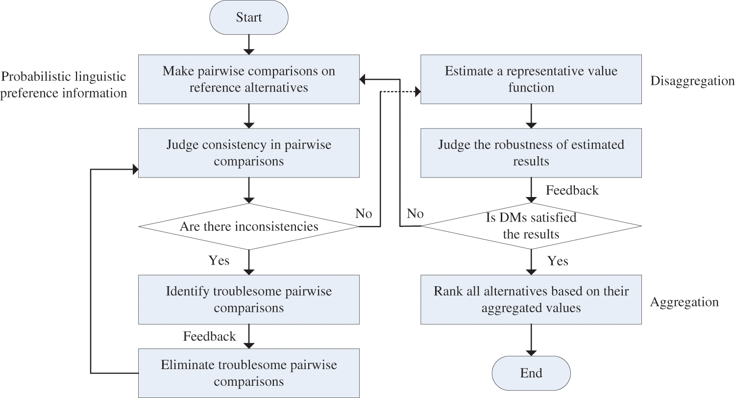
Figure 1: The framework of the proposed model

Overall, the proposed model consists of three stages, which can also be deemed as an interactive process between the analyst and DM. Firstly, the analyst introduces the DM the agricultural investment project selection problem, including the alternatives and criteria, and asks the DM to compare reference alternatives in pairs based on their overall performances. The DM can be asked to provide preferences through face-to-face questioning or questionnaires. The judgments provided by the DM are expressed as probabilistic linguistic term sets. The second stage (See Section 4.2 for details) is the management of inconsistencies in pairwise comparisons. The DM is recommended to change or remove some of the troublesome pairwise comparison values identified by Models 1 and 2. In the last stage (See Section 4.3 for details), the analyst estimates a value function through Model 3 based on consistent pairwise comparison values. Post-optimality analysis is used to check the robustness of estimations. The analyst returns the estimated result to the DM. If the DM is satisfied with the result, the preference disaggregation process is finished, and the estimated value function is used to make aggregation, such that the alternatives can be ranked based on their aggregated values. If the DM is not satisfied with the result, then (s)he is required to change original pairwise comparison values according to the estimated results, and the preference disaggregation process is repeated until the DM satisfies the estimated results. It should also be noted that the six optimization models (Models 1–6) introduced in this paper are all linear programming models that can be solved using mathematical programming solvers such as Gurobi and Cplex. In addition, none of the constraints in each model are conflicting or contradictory, so they always have solutions.

4.2 Managing Inconsistencies in Uncertain Pairwise Comparisons

There are three reasons which lead to the fact that we cannot find an additive value function to reproduce the pairwise comparisons provided by a DM [5,42]: (1) the DM’s preference model is not additive (which may occur when decision criteria are interactive); (2) the DM makes errors in the statements (e.g., stating ai∗≻av∗ but in fact ai∗∼av∗); and (3) the DM provides contradictory statements (e.g., providing ai∗≻av∗, av∗≻ak∗ and ak∗≻ai∗ at the same time) because of his/her limited ability to make holistic judgments on reference alternatives and unstable judgment policy. The first one is a technique problem, that is, the additive value function cannot model the DM’s preferences. Interested readers may refer to Liu et al. [32], which investigated non-additive preference models in preference disaggregation analysis. This study only focuses on multi-criteria ranking problems where the preference model is additive. Thus, the first scenario is not considered here. The last two reasons are subjective problems regarding unreliable judgments of the DM. In this sense, inconsistencies can be eliminated by dealing with troublesome pairwise comparisons.

To achieve this goal, the primary work is to formalize pairwise comparison values through the additive value function. When only considering “preference” and “indifference” relations, the following constraints can be established: (1) if ai∗≻av∗, then U(ai∗)>U(av∗), (2) if ai∗≺av∗, then U(ai∗)<U(av∗), and (3) if ai∗=av∗, then U(ai∗)≈U(av∗). When considering the intensities of preference relations, the semantics of each intensity expressed in linguistic terms (e.g., “slightly preferred”, and “strongly preferred”) needs to be specified to reflect the difference in values between the reference alternatives. According to the fuzzy linguistic theory [43], the semantics of a linguistic term can be explained by a triangular fuzzy number. Each linguistic term is described by numerical values in [−1, 1] and membership degrees. The numerical values represent the tendencies and intensities of the preference relation defined by the linguistic terms. The membership degree describes the possibility of a numerical value to the linguistic term. There is no clear boundary between the semantics of adjacent linguistic terms. Still, each linguistic term sα has a central value (i.e., the medium value of the triangular fuzzy number, denoted as u(sα)), which is a representative numerical meaning of the linguistic term. If a preference relation is expressed as sα, then the preference intensity is around u(sα), and almost between tα−1 and tα, ∀α≠0,−τ,τ, where u(s0)=0 and u(sα)<u(sα+1)≤1, ∀α∈{−τ,⋯,τ−1} [44].

We define a set of preference thresholds {t−τ−1, t−τ, ⋯, t−1, t1, ⋯, tτ, tτ+1}, satisfying 0<tα<tα+1≤tτ+1≤1, tα=−t−α,∀α∈{1,⋯,τ}. Especially, t1 is a small positive constant to define the indifference relation. If the difference between the global values of ai∗ and av∗, |U(ai∗)−U(av∗)|, is smaller than t1, then these two alternatives are indifferent. Overall, the preference relation of ai∗ over av∗ indicated by linguistic terms, sα,∀α∈{−τ,⋯,τ}, can be approximately represented by a pair of constraints based on a value function.

1.    (Indifference relation) α=0⇔|U(ai∗)−U(av∗)|≤t1;

2.    (Positive preference relation) 0<α≤τ−1⇔ tα<U(ai∗)−U(av∗)≤tα+1; α=τ⇔ tτ<U(ai∗)−U(av∗);

3.    (Negative preference relation) −τ+1≤α<0⇔ t−α<U(av∗)−U(ai∗)≤t−α+1; α=−τ⇔ tτ<U(av∗)−U(ai∗).

If the belief degree pαiv in the preference relation of ai∗ over av∗ being sα is smaller than 1, the constraints on the difference between the global values of ai∗ and av∗, U(ai∗)−U(av∗), should be relaxed. The lower the belief degree is, the looser the constraints should be. In this regard, the constraints on a probabilistic linguistic preference relation P(ai∗,av∗) can be set as Eq. (5).

EP(ai∗,av∗){(U(ai∗)−U(av∗))>pτivtτ, if pτiv>0pαiv(U(ai∗)−U(av∗))≤tα+1,(U(ai∗)−U(av∗))>pαivtα,∀α∈{1,⋯,τ−1}, if pαiv>0p0iv|U(ai∗)−U(av∗)|≤t1, if p0iv>0pαiv(U(av∗)−U(ai∗))≤t−α+1,(U(av∗)−U(ai∗))>pαivt−α,∀α∈{−τ+1,⋯,−1}, if pαiv>0(U(av∗)−U(ai∗))>p−τivtτ, if p−τiv>0(5)

If the constraints on all pairwise comparison values provided by the DM are feasible, then the preference information is consistent, and at least one value function is compatible with all the provided decision examples. Otherwise, incompatibility (i.e., inconsistent pairwise comparison information) exists. In this case, we can find a set of pairwise comparisons which make the constraints on the remaining pairwise comparison values are feasible when we remove them. Searching for the smallest number of troublesome pairwise comparison values is consistent with the idea that the DM first considers “less complex” ways to resolve inconsistencies [10]. The identification procedure to find troublesome pairwise comparison values can be performed by solving Model 1.

Model 1. MinF=∑ai∗,av∗∈AR∑α∈{−τ,⋯,τ}rαiv

s.t.

Ein1P{(U(ai∗)−U(av∗))+rτiv>pτivtτ, if pτiv>0pαiv(U(ai∗)−U(av∗))−rαiv≤tα+1,(U(ai∗)−U(av∗))+rαiv>pαivtα,∀α∈{1,⋯,τ−1}, if pαiv>0p0iv|U(ai∗)−U(av∗)|−r0iv≤t1, if p0iv>0pαiv(U(av∗)−U(ai∗))−rαiv≤t−α+1,(U(av∗)−U(ai∗))+rαiv>pαivt−α,∀α∈{−τ+1,⋯,−1}, if pαiv>0(U(av∗)−U(ai∗))+r−τiv>p−τivtτ,if p−τiv>0rαiv∈{0,1},∀α∈{−τ,⋯,τ}}∀ai∗,av∗∈AREM(C);∑j=1nwj=1,wj≥γ,∀j∈G

In Ein1P, the first part is about the constraints on pairwise comparisons between reference alternatives, expressed by the difference of global values of ai∗ and av∗ and preference thresholds. rαiv is a binary variable, i.e., rαiv=0 or 1. If the provided preference relation (sα(pαiv)) between ai∗ and av∗ conforms to the corresponding constraints, then rαiv=0; otherwise rαiv=1. Especially, when rαiv=1, the corresponding constraints are always satisfied and do not play a role in the estimation process. Therefore, with Model 1, we can get the minimum number of pairwise comparisons that lead to inconsistency. The second part is about the constraints on the marginal values of each criterion, as defined by Eq. (3), as well as the constraints on the trade-off weights of criteria. γ is a user-defined parameter to represent the minimum weight of each criterion.

There may be multiple subsets of troublesome pairwise comparisons that lead to inconsistency with the optimal objective function value of Model 1 being F∗. An intuitive goal of dealing with inconsistency is to maintain the original preference information provided by the DM as much as possible. We can find a value function that represents the most likely preference model with the minimum estimation error [6]. Pairwise comparison values that are not compatible with this value function can be identified as a representative option to remove inconsistency. The identification procedure can be performed by solving Model 2, which is a 0–1 mixed integer programming model.

Model 2. MinK=∑ai∗,av∗∈AR∑α∈{−τ,⋯,τ}λαivrαiv

s.t.

Ein2P{(U(ai∗)−U(av∗))+λτivrτiv>pτivtτ,if pτiv>0pαiv(U(ai∗)−U(av∗))−λαivrαiv≤tα+1,(U(ai∗)−U(av∗))+λαivrαiv>pαivtα,∀α∈{1,⋯,τ−1}, if pαiv>0p0iv|U(ai∗)−U(av∗)|−λ0ivr0iv≤t1, if p0iv>0pαiv(U(av∗)−U(ai∗))−λαivrαiv≤t−α+1,(U(av∗)−U(ai∗))+λαivrαiv>pαivt−α,∀α∈{−τ+1,⋯,−1}, if pαiv>0(U(av∗)−U(ai∗))+λ−τivr−τiv>p−τivtτ, if p−τiv>0rαiv∈{0,1},∀α∈{−τ,⋯,τ},∑ai∗,av∗∈AR∑α∈{−τ,⋯,τ}⁡rαiv≤F∗λαiv≥λ,∀α∈{−τ,⋯,τ}}∀ai∗,av∗∈AREM(C);∑j=1nwj=1,wj≥γ,∀j∈G

In Ein2P, the first part of the constraints is about the provided preference relation (sα(pαiv)) between each pair of reference alternatives, described by the estimation error λαivrαiv. λ is any positive number close to 0. It is required that the total number of troublesome pairwise comparisons is not larger than F∗, i.e., ∑ai∗,av∗∈AR∑α∈{−τ,⋯,τ}rαiv≤F∗. The second part is about the constraints on the marginal values and trade-off weights of criteria. With Model 2, we can find a subset of pairwise comparison values sα(pαiv) with rαiv=1, for α∈{−τ,⋯,τ}, ai∗,av∗∈A, which are not compatible with the estimated value function.

Overall, the procedure to manage inconsistencies in pairwise comparison values is presented as follows:

Step 2.1. The analyst uses Model 1 to check if the pairwise comparisons are consistent. If F∗=0, the preference information is consistent, and the process of dealing with inconsistency is finished. Otherwise, the preference information is inconsistent, and F∗ is the minimum number of pairwise comparisons that lead to inconsistency, and then go to the next step.

Step 2.2. The analyst uses Model 2 to identify a subset of troublesome pairwise comparisons, and return such information to the DM. Go to the next step.

Step 2.3. The DM is required to change or remove the preference statements on all or some of the identified troublesome pairwise comparisons. Go to Step 2.1.

If multiple DMs participate in decision-making, we follow the aforementioned steps to assess consistency in the pairwise comparisons provided by each DM. Once the pairwise comparisons of all DMs satisfy consistency, we integrate their comparisons. In this process, if multiple DMs simultaneously compare a pair of reference alternatives, their collective opinion is also expressed as a probabilistic linguistic term set. The probability of each linguistic term in this set is the average of the probabilities corresponding to that linguistic term provided by different DMs (Details can be found in [42]). In this setting, the collective opinion of DMs is applied for preference disaggregation. It should be noted that when dealing with large numbers of DMs, individually interacting with them to revise troublesome pairwise comparisons is costly. Therefore, we may consider deleting the identified troublesome pairwise comparisons in Step 2.2 without further requiring the DMs’ interaction with the analyst.

4.3 Deriving a Value Function through Preference Disaggregation

To model the uncertain preference intensity between a pair of reference alternatives quantitatively, we need to analyze the semantics of probabilistic linguistic information. The expected utility theory [45] pointed out that the utility of a distribution can be defined as the weighted sum of the utilities of the states in a set, and the weight is the probability assigned to the state. A probabilistic linguistic term set is a distribution regarding a linguistic term set, and each linguistic term can be regarded as a state in the set. Thus, the value U¯(ai∗,av∗) of a piece of probabilistic linguistic preference information can be defined as Eq. (6), where pαiv/∑α=−ττpαiv is a normalized form of the probability of the linguistic term sα, such that the distribution of the probabilities of linguistic terms is complete. The representative numerical meaning u(sα) of sα can represent its semantics, which satisfies sα≤sβ if and only if u(sα)≤u(sβ). Suppose that the values in each subinterval are linearly distributed, and the semantics u(sα) of sα can be set as u(sα)=(tα+tα+1)/2. U¯(ai∗,av∗)∈[−1,1] represents the most likely difference between the global values of the reference alternatives ai∗ and av∗. In other words, the value difference U(ai∗)−U(av∗) is around U¯(ai∗,av∗), such that Eq. (7) holds, where εiv+ and εiv− are small positive numbers. There is U¯(ai∗,av∗)=−U¯(av∗,ai∗).

U¯(ai∗,av∗)=∑α=−ττu(sα)×(pαiv/∑α=−ττpαiv)(6)

U(ai∗)−U(av∗)+εiv+−εiv−=U¯(ai∗,av∗)(7)

The value function should satisfy the setting in which the value difference of each pair of reference alternatives is as close as possible to the semantics of their probabilistic linguistic preference information. In this sense, εiv+ and εiv− can be taken as the underestimation and overestimation errors, respectively. Estimating a value function can be achieved through linear programming to minimize the total estimation errors for all pairwise comparison values. Thus, Model 3 is constructed, where the first part of the constraints is basic requirements for a value function that describes the preference relation between each pair of reference alternatives. The second part of the constraints is critical for estimating a value function that makes the difference between the global values of each pair of reference alternative close to the semantics of their probabilistic linguistic preference information provided by the DM. The third part of the constraints is about the marginal values of criteria. The fourth one is about the semantics of linguistic terms, defined by adjacent preference thresholds. The last two parts of constraints are about the values of decision variables, including the weights of criteria and the estimation errors.

Model 3. MinT=∑ai∗,av∗∈A∗(εiv++εiv−)

s.t.: EreP{EP(ai∗,av∗),∀ai∗,av∗∈ARU(ai∗)−U(av∗)+εiv+−εiv−=U¯(ai∗,av∗),∀ai∗,av∗∈AREM(C)u(sα)=(tα+tα+1)/2,u(s−α)=−u(sα),α∈{1,2,⋯,τ}∑j=1nwj=1,wj≥γ,∀j∈Gεiv+,εiv−≥0,∀ai∗,av∗∈AR

However, due to the uncertainty in the preference information provided by the DM, the value function corresponding to the optimal solution obtained in Model 3 does not always reflect the DM’s preference structure well. In this sense, we need to explore suboptimal solutions in the neighborhood of the optimal solution obtained by Model 3. Therefore, we conduct post-optimality analysis by Model 4, with the objective of minimizing and maximizing the trade-off weight of each criterion, respectively [29]. It aims to explore other possible values of the variables with an additional constraint as T≤(1+k)T∗, where T∗ is the objective value of Model 3, and k is a user-defined small positive number.

Model 4. Max/Min wj

s.t.: {ErePF≤(1+k)F∗

5  Case Study: Agricultural Investment Project Selection

To demonstrate the applicability of the proposed model, we elaborate a case study on agricultural investment project selection.

5.1 Case Description

The local government in a region prioritizes agricultural development and has established a Rural Revitalization Investment Fund. This fund selects outstanding agricultural projects for annual funding, focusing on key sectors such as local characteristic industries, modern farming, agricultural product processing and distribution, rural leisure tourism, new service industries, and the information industry. The fund is committed to providing capital support for rural revitalization based on mature, promising, and market-oriented industrial projects. After an initial screening, the fund managers have shortlisted 25 project applications (P1–P25) as candidates and plan to choose 5 projects for funding. They have decided to use the following 5 decision criteria to evaluate the projects after conducting in-depth project analysis:

1.    Cost of capital (cost criterion): the capital cost of the agricultural industry investment funds.

2.    Ecological cost (cost criterion): the cost of ecological environmental damage. Due to the large use of natural resources such as land, agricultural enterprises would inevitably affect the ecological environment system formed over a long period and even change the ecological balance of the surrounding land.

3.    Return on investment (benefit criterion): the economic return value through the investment.

4.    Industrial driving index (benefit criterion): the economic driving force of agricultural enterprises (projects) can be divided into three aspects: regional driving force, industrial driving force, and technological driving force. It reflects the economic driving effect of investments.

5.    Risk level (target criterion): the object of the agricultural industry investment fund is the agricultural enterprises in the initial stage, which belongs to the venture capital fund. Investment risk, including natural risk, operation risk, and market risk, is an important factor in evaluating projects. Here the risk of projects is divided into five levels. Different DMs have different attitudes to risk.

The performance values of the 25 projects under the five criteria were collected from the materials provided by agricultural enterprises (see Table 3). The first two criteria are in cost form, while the next two criteria are in benefit form. The last criterion is a target-type criterion, and its optimal value is not the minimum or maximum, but rather between them. Suppose that the optimal value of the last criterion is 3.

5.2 Resolving Process Based on the Proposed Model

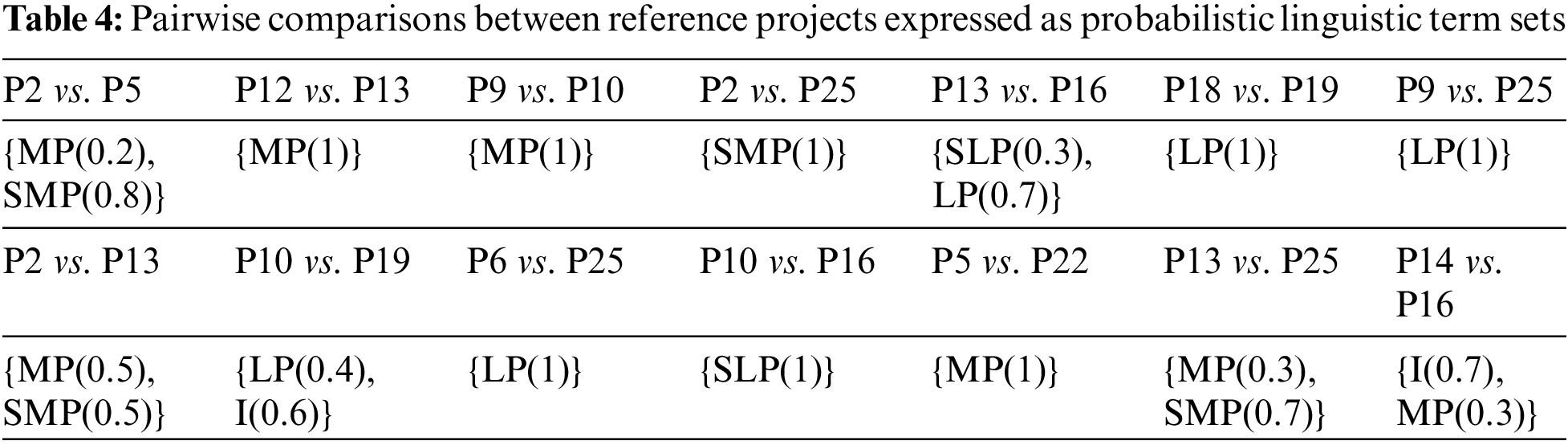
To assess the alternative projects rigorously, this study employs the proposed method to develop a decision model, offering decision support. The first step involves inviting a DM to conduct pairwise comparisons of the alternative projects (s)he is familiar with. The linguistic term set for pairwise comparisons is set to {SLP, LP, I, MP, SMP}. The judgments are shown in Table 4. There are uncertain preference intensities between some reference alternatives. For example, the possible preference intensities between P2 and P5 are MP and SMP, and the belief degree of the DM in MP is 0.2, and that in SMP is 0.8.

Before the solving process is performed, the parameters in the model need to be determined. Considering that all the five criteria have an impact on the decision result, we set the weight of each criterion to be greater than 0.05, i.e., γ=0.05, which is lower than the average weight 0.2. To measure the marginal values of the first four criteria, we set the number of subintervals in the marginal value function to a moderate value, 3. Given that the last criterion is valued between 1 and 5, we set each risk level as a segment point of the marginal value function of the criterion. For generality, the minimum difference between each pair of adjacent segment points is set to 0.2. In addition, the preference thresholds are set to t1=0.05, t2=0.15, and t3=0.25. It means that, if the difference in values between a pair of alternatives is less than 0.05, they are indifferent; if their difference is greater than 0.15, they have a strong preference relation; otherwise, their preference relation is weak. The parameter for post-optimality analysis is set as k=0.01.

Using Model 1 to test the consistency of the original pairwise comparison values provided by the DM, we find at least one troublesome pairwise comparison value. Then, using Model 2, the most likely troublesome pairwise comparison value is identified as the preference of P2 over P25, i.e., {MP(1)}. After the feedback, the DM changes the preference of P2 over P25 to {SMP(1)}. Based on Model 1, we find that the pairwise comparison values after update are consistent. Then, the updated pairwise comparison values are disaggregated through Model 3, and a value function is obtained to describe the preference structure of the DM. The weights of five criteria are estimated to be 0.29, 0.09, 0.3, 0.14, and 0.19, respectively, indicating that the DM pays the most attention to the return on investment and cost of capital, and pays the least attention to the ecological cost. Except for the two cost criteria, the other criteria have different marginal utility functions, as shown in Fig. 2. According to the estimated value function, criterion values of each alternative are aggregated to determine the ranking of all alternatives. The top five alternatives are P2, P12, P14, P16 and P13, which can be recommended to the DM for project investment.

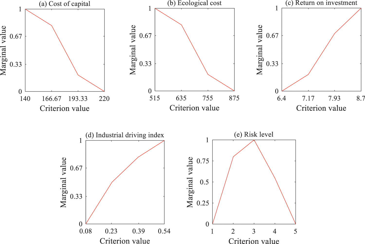
Figure 2: The marginal value functions of five criteria

We further use Model 4 to carry out post-optimality analysis for the preference parameters. The estimated weight of each criterion is shown in Fig. 3. Except for the industrial driving index, the weights of other four criteria are relatively stable. At the same time, the marginal value functions of all criteria are stable. We average the ranks of alternatives obtained in the post-optimality analysis. The results also show that the top five alternatives are P2, P12, P14, P16, and P13, respectively, indicating that the estimated value function is robust.

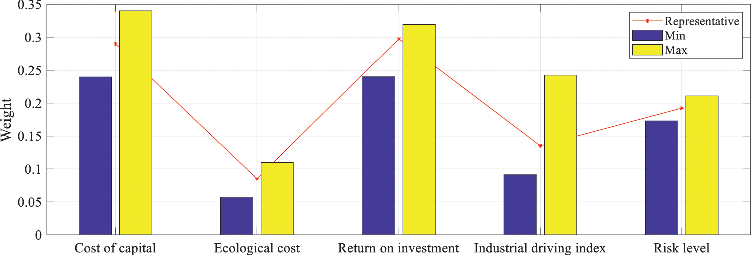
Figure 3: The maximum, minimum, and representative weights of criteria

5.3 Comparative Analysis

Based on the case study, this section compares the proposed model with a UTA-like method and a preference disaggregation model without consistency management.

5.3.1 Preference Disaggregation by a UTA-Like Method

In the UTA method as well as most of its extensions, the preference relation between reference alternatives is expressed as an “indifferent (I)” or “preferred (P)” relation [25]. To illustrate the necessity of considering the uncertainty of preference intensities between reference alternatives in preference disaggregation analysis, we re-invite the DM to provide preferences based on the linguistic term set {I, P}, as shown in Table 5.

In the original version of UTA [29], an error function to be minimized is introduced for each reference alternative. This error function is not sufficient to completely minimize the error. To solve this problem, the UTASTAR method [46] uses a double positive error function. According to the UTASTAR method, Model 5 can be established to estimate the DM’s preference model.

Model 5. MinT=∑ai∗,av∗∈AR(εiv++εiv−)

s.t. E1p{U(ai∗)−U(av∗)+εiv+>=δ,ifai∗≻av∗|U(ai∗)−U(av∗)|−εiv−=0,ifai∗∼av∗}∀ai∗,av∗∈AREM(C)∑j=1nwj=1,wj≥γ,∀j∈Gεiv+,εiv−≥0,∀ai∗,av∗∈AR

The decision variables include the weights of criteria (i.e., wj, j=1,2,⋯,n) and estimation errors (i.e., εiv+, εiv−, ∀ai∗,av∗∈AR). The first constraint (i.e., U(ai∗)−U(av∗)+εiv+>=δ) is about the difference between the overall values of two reference alternatives (ai∗ and av∗) if they have a preferred relation (i.e., ai∗≻av∗), where εiv+ is the underestimation error for the preference of ai∗ over av∗. The positive parameter δ has the same meaning as the preference threshold t1. If the difference between the overall values of two alternatives is greater than this parameter, they have a preferred relation; conversely, they have an indifferent relation. For this case study, we set δ=0.05. The second constraint (i.e., |U(ai∗)−U(av∗)|−εiv−=0) is about the difference between the overall values of two reference alternatives if they have an indifferent relation (i.e., ai∗∼av∗), where εiv− is the overestimation error for the preference of ai∗ over av∗. The constraint EM(C) is about the marginal values of criteria, as defined by Eq. (4). The last two constraints are about the value range of decision variables.

Through Model 5, the weights of the five criteria are estimated to be 0.36, 0.05, 0.25, 0.13 and 0.21, respectively. The top five alternatives are P12, P2, P14, P16, and P13, respectively, which are slightly different from the results obtained by our proposed model.

5.3.2 Preference Disaggregation without Consistency Management

An important part of our proposed preference disaggregation technique is to deal with inconsistent preference information. To illustrate the need to eliminate inconsistent preferences before preference disaggregation, we compare the results obtained by the proposed model with those obtained by the preference disaggregation analysis based on inconsistent preference information. In the model for comparative analysis, the constraints on the value function to be compatible with all pairwise comparison values are not considered, so Model 6 is established. Model 6 does not contain the first part of the constraints (i.e., EP(ai∗,av∗),∀ai∗,av∗∈AR) in Model 3, and all other constraints and decision variables are consistent with Model 3.

Model 6. MinT=∑ai∗,av∗∈AR(εiv++εiv−)

s.t.: E2P{U(ai∗)−U(av∗)+εiv+−εiv−=U¯(ai∗,av∗),∀ai∗,av∗∈AREM(C)∑j=1nwj=1,wj≥γ,∀j∈Gu(sα)=(tα+tα+1)/2,u(s−α)=−u(sα),∀α∈{1,2,⋯,τ}εiv+,εiv−≥0,∀ai∗,av∗∈AR

Through Model 6, the weights of five criteria are estimated to be 0.13, 0.12, 0.27, 0.30, and 0.18, respectively. The top five alternatives are P2, P14, P12, P16, and P1, respectively.

5.3.3 Discussions

Table 6 shows the global values and ranks of the projects estimated by the three preference disaggregation models. In the following, a detailed comparison of the results obtained from the three models is presented, and the advantages of the proposed model are highlighted:

(1) According to the Pearson correlation coefficient [47], we calculate the similarity between the ranking obtained by the UTA method and the ranking obtained by our proposed model. The result is 0.965. This high similarity indicates that the proposed model is reliable. In addition, the results of the two methods are slightly different as the uncertainty in preference intensities is considered in our proposed model. For example, the global values of P6, P25, and P2 obtained by our proposed model are 0.486, 0.586, and 0.827, respectively, and those obtained by the UTA method are 0.495, 0.671, and 0.833, respectively. The results of the proposed model conform to the original opinion of the DM, that is, the preference intensity of P2 over P25 is greater than the preference intensity of P25 over P6. However, the results of the UTA method do not conform to this opinion. Therefore, when the DM is allowed to express preferences as probabilistic linguistic information, the results of preference disaggregation can be more compatible with the DM’s underlying preference model.

(2) The Pearson correlation coefficient between the ranking results obtained by Model 6 and those obtained by our proposed model is 0.8, indicating that there is a significant difference between the results obtained by the two models. The value function estimated by Model 6 is not compatible with all the pairwise comparison values provided by the DM. For example, the DM stated that P9 is preferred to P10; however, the global value (0.352) of P9 estimated by Model 6 is smaller than that (0.394) of P10. In this regard, we can conclude that the use of inconsistent preference information can mislead the estimation results of preference disaggregation analysis.

6  Conclusions

This study proposes a preference disaggregation method to solve multi-criteria ranking problems with inconsistent preferences under uncertainty. The underlying preference model was set as an additive value function consisting of a set of piecewise linear marginal value functions that measure the values of criteria that may be in benefit, cost, or target form. Two 0–1 mixed integer programming models were constructed to check and eliminate inconsistencies in the holistic judgments of reference alternatives provided by the DM. A linear programming model was established to infer a value function that is not only compatible with all the holistic judgments but also can reproduce the desired preference relations between reference alternatives as much as possible. Based on the semantics of linguistic terms and the DM’s belief degrees in each term, the holistic judgments were transformed into the constraints in these optimization models. A case study on agricultural investment project selection demonstrated the desirable characteristics of the proposed method. Overall, the proposed model provides impact and insights for dealing with agricultural investment project selection problems with uncertainty. The implementation of the proposed model not only mitigates the complexity of evaluation for DMs but also minimizes inconsistencies in collective evaluation information. Furthermore, this approach enables DMs to utilize a blend of linguistic and probabilistic expressions that they are familiar with during the evaluation process.

Future research can be carried out in the following three aspects. (1) Future research into project evaluation and selection problems, where criteria interact, could harness non-additive value functions such as Choquet integrals and multilinear utility functions to portray the preference structure of DMs. (2) Future research into MCDM problems that involve a large number of DMs should take into account the trade-off between the consistency of decision information and the cost of interaction to achieve consensus. (3) For MCDM problems with large-scale historical decision examples, cross-validation can be investigated to evaluate the preference disaggregation framework objectively. In this way, the fitting and prediction ability of the estimated preference models can be measured.

Acknowledgement: We would like to thank the anonymous reviewers who have helped to improve the paper.

Funding Statement: None.

Author Contributions: The authors confirm contribution to the paper as follows: study conception and design: Xingli Wu; data collection: Xingli Wu, Shuxian Sun; analysis and interpretation of results: Xingli Wu, Shuxian Sun; draft manuscript preparation: Xingli Wu, Huchang Liao, Shuxian Sun, Zhengjun Wan. All authors reviewed the results and approved the final version of the manuscript.

Availability of Data and Materials: All data are available in this paper.

Conflicts of Interest: The authors declare that they have no conflicts of interest to report regarding the present study.

1“Inconsistent” here means that a DM provides decision examples that are incompatible with a single preference model.

2Cost benefit analysis in World Bank projects. Washington DC; 2010. Available: https://openknowledge.worldbank.org/handle/10986/2561.

References

1. Yet, B., Lamanna, C., Shepherd, K. D., Rosenstock, T. S. (2020). Evidence-based investment selection: Prioritizing agricultural development investments under climatic and socio-political risk using Bayesian networks. PLoS One, 15(6), e0236909. https://doi.org/10.1371/journal.pone.0234213 [Google Scholar] [PubMed] [CrossRef]

2. Cinelli, M., Kadziński, M., Gonzalez, M., Słowiński, R. (2020). How to support the application of multiple criteria decision analysis? Let us start with a comprehensive taxonomy. Omega, 96, 102261. https://doi.org/10.1016/j.omega.2020.102261 [Google Scholar] [PubMed] [CrossRef]

3. Lindell, M. K. (2014). Judgment and decision making. In: Webster, M., Sell, J. (Eds.Laboratory experiments in the social sciences, pp. 403–431. San Diego, CA, USA: Academic Press. [Google Scholar]

4. Dembczyński, K., Greco, S., Słowiński, R. (2009). Rough set approach to multiple criteria classifications with imprecise evaluations and assignments. European Journal of Operational Research, 198(2), 626–636. [Google Scholar]

5. Greco, S., Mousseau, V., Słowiński, R. (2010). Multiple criteria sorting with a set of additive value functions. European Journal of Operational Research, 207(3), 1455–1470. [Google Scholar]

6. Kadziński, M., Cinelli, M., Ciomek, K., Coles, S. R., Nadagouda, M. N. et al. (2018). Co-constructive development of a green chemistry-based model for the assessment of nanoparticles synthesis. European Journal of Operational Research, 264, 472–490. [Google Scholar] [PubMed]

7. Tversky, A., Kahneman, D. (1974). Judgment under uncertainty: Heuristics and biases. Science, 85, 1124–1131. [Google Scholar]

8. Kahneman, D., Rosenfield, A. M., Gandhi, L., Blaser, T. (2016). Reducing noise in decision making. Harvard Business Review, 94, 36–45. [Google Scholar]

9. Kadziński, M., Badura, J., Figueira, J. R. (2020). Using a segmenting description approach in multiple criteria decision aiding. Expert Systems with Applications, 147, 113186. https://doi.org/10.1016/j.eswa.2020.113186 [Google Scholar] [CrossRef]

10. Mousseau, V., Figueira, J., Dias, L., da Silva, C. J., Clı́maco, J. (2003). Resolving inconsistencies among constraints on the parameters of an MCDA model. European Journal of Operational Research, 147(1), 72–93. [Google Scholar]

11. Cai, F. L., Liao, X. W., Wang, K. L. (2012). An interactive sorting approach based on the assignment examples of multiple decision makers with different priorities. Annals of Operations Research, 197(1), 87–108. [Google Scholar]

12. Machina, M. J., Schmeidler, D. (1992). A more robust definition of subjective probability. Econometrica, 60(4), 745–780. [Google Scholar]

13. Pang, Q., Wang, H., Xu, Z. S. (2016). Probabilistic linguistic term sets in multi-attribute group decision making. Information Sciences, 369, 128–143. [Google Scholar]

14. Zhang, Y. X., Xu, Z. S., Liao, H. C. (2018). An ordinal consistency-based group decision making process with probabilistic linguistic preference relation. Information Sciences, 467, 179–198. [Google Scholar]

15. Branca, G., Lipper, L., Sorrentino, A. (2015). Cost-effectiveness of climate-related agricultural investments in developing countries: A case study. New Medit, 14(2), 4–12. [Google Scholar]

16. Geleta, M. T. (2018). Manage responsible agricultural investments using open source solution. African Journal on Land Policy and Geospatial Sciences, 1(2), 93–101. [Google Scholar]

17. Mutenje, M. J., Farnworth, C. R., Stirling, C., Thierfelder, C., Mupangwa, W. et al. (2019). A cost-benefit analysis of climate-smart agriculture options in Southern Africa: Balancing gender and technology. Ecological Economics, 163, 126–137. [Google Scholar]

18. Patari, E., Karell, V., Luukka, P., Yeomans, J. S. (2018). Comparison of the multicriteria decision-making methods for equity portfolio selection: The U.S. evidence. European Journal of Operational Research, 265(2), 655–672. [Google Scholar]

19. Goers, J., Horton, G. (2023). Project selection in a biotechnology startup using combinatorial acceptability analysis. Decision Making: Applications in Management and Engineering, 6(2), 828–852. [Google Scholar]

20. Shepherd, K., Hubbard, D., Fenton, N., Claxton, K., Luedeling, E. et al. (2015). Policy: Development goals should enable decision-making. Nature, 523, 152–154. [Google Scholar] [PubMed]

21. Phurksaphanrat, B., Panjavongroj, S. (2023). A hybrid method for occupations selection in the bio-circular-green economy project of the national housing authority in Thailand. Decision Making: Applications in Management and Engineering, 6(2), 177–200. [Google Scholar]

22. Volden, G. H. (2019). Assessing public projects’ value for money: An empirical study of the usefulness of cost-benefit analyses in decision-making. International Journal of Project Management, 37(4), 549–564. [Google Scholar]

23. Almeida-Filho, A. T. D., de Lima Silva, D. F., Ferreira, L. (2021). Financial modelling with multiple criteria decision making: A systematic literature review. Journal of the Operational Research Society, 72(10), 2161–2179. [Google Scholar]

24. Karasakal, E., Eryılmaz, U., Karasakal, O. (2022). Ranking using PROMETHEE when weights and thresholds are imprecise: A data envelopment analysis approach. Journal of the Operational Research Society, 73(9), 1978–1995. [Google Scholar]

25. Doumpos, M., Grigoroudis, E., Matsatsinis, N. F., Zopounidis, C. (2022). Preference disaggregation analysis: An overview of methodological advances and applications. In: Greco, S., Mousseau, V., Stefanowski, J., Zopounidis, C. (Eds.Intelligent decision support systems, pp. 73–100. Cham: Springer. [Google Scholar]

26. Doumpos, M., Figueira, J. R. (2019). A multicriteria outranking approach for modeling corporate credit ratings: An application of the ELECTRE TRI-NC method. Omega, 82, 166–180. [Google Scholar]

27. Liu, J. P., Liao, X. W., Huang, W., Liao, X. Z. (2019). Market segmentation: A multiple criteria approach combining preference analysis and segmentation decision. Omega, 83, 1–13. [Google Scholar]

28. Wu, X. L., Liao, H. C. (2021). Learning judgment benchmarks of customers from online reviews. OR Spectrum, 43, 1125–1157. [Google Scholar]

29. Jacquet-Lagrèze, E., Siskos, Y. (1982). Assessing a set of additive utility functions for multicriteria decision making: The UTA method. European Journal of Operational Research, 10(2), 151–164. [Google Scholar]

30. Hu, J., Mehrotra, S. (2015). Robust decision making over a set of random targets or risk-averse utilities with an application to portfolio optimization. IIE Transactions, 47(4), 358–372. [Google Scholar]

31. Jacquet-Lagrèze, E. (1995). An application of the UTA discriminant model for the evaluation of R&D projects. In: Pardalos, P. M., Siskos, Y., Zopounidis, C. (Eds.Advances in multicriteria analysis, pp. 203–211. Dordrecht: Kluwer Academic Publishers. [Google Scholar]

32. Liu, J. P., Kadziński, M., Liao, X. W., Mao, X. X. (2021). Data-driven preference learning methods for value-driven multiple criteria sorting with interacting criteria. INFORMS Journal on Computing, 33(2), 419–835. [Google Scholar]

33. Kadziński, M., Tervonen, T., Figueira, J. R. (2015). Robust multi-criteria sorting with the outranking preference model and characteristic profiles. Omega, 55, 126–140. [Google Scholar]

34. Lolli, F., Balugani, E., Ishizaka, A., Gamberini, R., Butturi, M. A. et al. (2019). On the elicitation of criteria weights in PROMETHEE-based ranking methods for a mobile application. Expert Systems with Applications, 120, 217–227. [Google Scholar]

35. Greco, S., Słowiński, R., Zielniewicz, P. (2013). Putting dominance-based rough set approach and robust ordinal regression together. Decision Support Systems, 54(2), 891–903. [Google Scholar]

36. Buğdaci, A. G., Köksalan, M., Özpeynirci, S., Serin, Y. (2013). An interactive probabilistic approach to multi-criteria sorting. IIE Transactions, 45(10), 1048–1058. [Google Scholar]

37. Zheng, J., Lienert, J. (2018). Stakeholder interviews with two MAVT preference elicitation philosophies in a Swiss water infrastructure decision: Aggregation using SWING-weighting and disaggregation using UTAGMS. European Journal of Operational Research, 267(1), 273–287. [Google Scholar]

38. Corrente, S., Greco, S., Kadziński, M., Słowiński, R. (2013). Robust ordinal regression in preference learning and ranking. Machine Learning, 93(2–3), 381–422. [Google Scholar]

39. Kadziński, M., Tervonen, T. (2013). Stochastic ordinal regression for multiple criteria sorting problems. Decision Support Systems, 55(1), 55–66. [Google Scholar]

40. Kadziński, M., Greco, S., Słowiński, R. (2012). Selection of a representative value function in robust multiple criteria ranking and choice. European Journal of Operational Research, 217(3), 541–553. [Google Scholar]

41. Keeney, R. L., Raiffa, H. (1993). Decisions with multiple objectives: Preferences and value trade-offs. Cambridge: Cambridge University Press. [Google Scholar]

42. Wu, X. L., Liao, H. C., Zhang, C. H. (2024). Preference disaggregation analysis for sorting problems in the context of group decision-making with uncertain and inconsistent preferences. Information Fusion, 101, 102014. [Google Scholar]

43. Zadeh, L. A. (1975). The concept of a linguistic variable and its applications to approximate reasoning—I. Information Sciences, 8(3), 199–249. [Google Scholar]

44. Wu, X. L., Liao, H. C. (2023). Value-driven preference disaggregation analysis for uncertain preference information. Omega, 115, 102793. [Google Scholar]

45. von Neumann, J., Morgenstern, O. (1947). Theory of games and economic behavior, 2nd edition. Princeton, New Jersey: Princeton University Press. [Google Scholar]

46. Siskos, Y., Yannacopoulos, D. (1985). UTASTAR: An ordinal regression method for building additive value functions. Investigaçao Operacional, 5(1), 39–53. [Google Scholar]

47. Liao, H. C., Wu, X. L. (2020). DNMA: A double normalization-based multiple aggregation method for multi-expert multi-criteria decision making. Omega, 94, 102058. https://doi.org/10.1016/j.omega.2019.04.001 [Google Scholar] [CrossRef]