Cross-Dimension Attentive Feature Fusion Network for Unsupervised Time-Series Anomaly Detection

1  Introduction

Anomaly detection aims to find data points that significantly deviate from other samples in the same data group [1], which has been widely studied in diverse research areas and application domains [2,3]. Time series data tracks samples over time in temporal order, collected using field-deployed sensors that monitor the status of systems or services in the manufacturing industry [4]. Detecting anomalies in time series is a crucial task for monitoring various statuses and assisting the failure troubleshooting [5], thus preventing system failure and reducing system maintenance costs [6]. In the unsupervised setting, it is expected to detect anomalous events in time series without annotation. Given the advances in sensing technology, collecting time series data has become easier and faster in various fields [7], thus, there is an urgent need to develop effective methods that can precisely detect anomalies in time series.

Given the intricate dependencies among elements in time series data, many existing models struggle to capture complex relationships, leading to suboptimal detection performance. Following this research direction, many efforts have been made to mitigate this gap. In particular, machine learning methods [8,9] have been investigated in time series anomaly detection. In [10], a fast Fourier transform is utilized to extract features, and a Bacterial Foraging Algorithm (BFA)-Gaussian support vector classifier machine (GSVCM) model is introduced for analyzing electromyography (EMG) signals. In [11], spectrogram features, including short-time Fourier transform (STFT) and continuous wavelet transform (CWT), are exploited. Subsequently, a time-frequency approach called modified S-transform is introduced, which studies the phase coupling between two or more different spatially recorded entities with non-stationary characteristics. Also, K-Nearest Neighbor (KNN) [12] and Random Forest (RF) [13] are explored for time series anomaly detection using Dynamic Time Warping (DTW) or Principal Component Analysis (PCA) pre-processed features. Although these methods have made considerable progresses in time series anomaly detection, the need for domain knowledge in feature extraction generally limits their capability to capture dependencies and complex patterns in time series data, thereby impeding anomaly detection performance.

Deep learning methods have demonstrated significant success in various domains [14,15], including computer vision [16], speech recognition [17] and natural language processing [18]. This trend has garnered considerable attention in the field of time series analysis [19]. In [20], a Convolutional Neural Network (CNN) combined with a multiclass SVM is adopted for early anomaly diagnosis problems, showing superior performance compared to conventional SVM, KNN and traditional CNN. In another study [21], CNN and Recurrent Neural Network (RNN) are integrated to detect anomalies in Internet of Things (IoT) [22] time series, in which spatial and temporal features are extracted by CNN and recurrent autoencoder, respectively. In [23], a multi-head CNN-RNN model is assessed against a real industrial case study, processing each sensor with independent convolutions and requiring no pre-processing. Additionally, Generative Adversarial Networks (GANs) have been explored for time series anomaly detection in an unsupervised manner [24], where 1D CNN and Gated Recurrent Unit (GRU) are adopted as generator and discriminator, respectively. After training, the reconstruction error can serve as an informative indicator for determining whether a certain sample of the time series is anomalous. Furthermore, Variational AutoEncoders (VAEs) [25] have been adopted for learning lower-dimensional latent representations of video object trajectories, and then anomaly identification is achieved based on reconstruction loss. Given the advantage of automatic feature learning, deep learning models have made noticeable progresses in time series anomaly detection and considerably improved the performance. However, because of the locality property of convolution and sequential computation paradigm of recurrent models [26], capturing long-term dependencies remains challenging, presenting an obstacle to further improving the performance.

Recently, Transformers utilizing attention mechanism [27] have gained widespread use for modeling sequential data [17,18], achieving impressive results and outperforming RNNs and CNNs in natural language processing and computer vision tasks [18,28]. The attention mechanism allows the model to simultaneously focus on essential parts while ignoring the irrelevant segments in the sequence, independent of the sequence length, thus providing superior performance in modeling long sequences. In time series analysis, Transformer-based models have also demonstrated their effectiveness in capturing the long-term temporal dependencies among time points [29–31]. However, as the main working power of Transformers, the multi-head self-attention mechanism is permutation-invariant to some extent. Since time series analysis is inherently sensitive to the order of a continuous set of points, it inevitably suffers from temporal information loss, resulting in inferior performance [32]. In this paper, we propose a cross-dimension attentive feature fusion network called CAFFN. This network automatically extracts features from raw data in multiple dimensions, each possessing different levels of locality properties. These features are then adaptively fused for time series anomaly detection. This design enables the learning of local and global temporal representations in 1D and 2D spaces, allowing for more effective capture of the complex patterns and dependencies in time series. The contributions of this paper are summarized as follows:

•   A cross-dimension attentive feature fusion network model is proposed, which learns and fuses time series features from multiple dimensions with different levels of locality properties.

•   A mixing strategy is introduced to model the dependencies at both series and feature levels, which can effectively capture the correlations in time series data.

•   Evaluation on benchmark datasets shows that the proposed CAFFN achieves superior performance compared to other competing time series anomaly detection methods.

2  Related Works

2.1 Anomaly Detection

Anomaly detection refers to the identification of patterns in data that do not conform to the expected behavior, a challenge that has been actively explored for several decades [33]. Due to its broad applicability in diverse domains such as financial surveillance, risk management, health and medical risk, and AI safety, anomaly detection plays an increasingly crucial role in real-world scenarios. Various detectors have been investigated, which have made considerable progress in anomaly detection tasks. Supervised models assume the availability of a training dataset with labeled instances for both normal and anomaly classes [34]. However, obtaining accurate and representative labels can be challenging. As a trade-off solution, semi-supervised anomaly detection assumes that the training data has labeled instances only for the normal class, thus obviating the need for labels for the anomaly class [34]. In an extreme case, unsupervised anomaly detection [35,36] does not require any labeled data, with the assumption that normal instances are far more frequent than anomalies in the test data [37]. Consequently, a variety of machine learning and deep learning methods have been developed for anomaly detection.

2.2 Machine Learning Methods

Machine learning has been widely investigated for time series analysis. For instance, the autocorrelation function and spectrum of the stationary process were explored to learn temporal dynamics [38], and exponential smoothing [39] was used with Fourier functions of time to model seasonality in time series. Also, exponentially weighted moving averages were adopted for sales data analysis [40]. Considering the irregular properties of time series, the Kalman filter was introduced to deal with situations in which the observations were irregularly spaced [41]. In addition, Gaussian processes and their extension deep Gaussian processes [42] have been employed for time-series prediction [43], providing a probabilistic means to model the temporal patterns in sequential data. Support vector regression [44,45] has demonstrated superiority over other nonlinear techniques, such as multi-layer perceptions, especially when dealing with time series data sampled from nonlinear and non-stationary system processes. Furthermore, K-Nearest Neighbor (KNN) [12] and Random Forest (RF) [13] have also been assessed for time series anomaly detection tasks. Although machine learning methods have achieved considerable success in this field, the performance of machine learning pipelines heavily relies on domain knowledge and handcrafted feature design, such as short-time Fourier transform and continuous wavelet transform [10,11]. This inevitably leads to information loss, hampering detection performance.

2.3 Deep Learning Methods

By stacking multiple layers and imposing connection restrictions, deep neural networks [46–48] have shown remarkable potential in learning nonlinear mapping and features from raw time series data without any prior domain knowledge. In [49], Hierarchical Temporal Memory (HTM) was employed for anomaly detection in streaming applications, where an online processing paradigm was presented for handling streaming data from sensors. In [50], the Restricted Boltzmann Machine (RBM) was utilized to learn system-wide patterns in distributed cyber-physical systems in a data-driven fashion. It demonstrated its capability to capture multiple nominal modes with one energy-based probabilistic graphical model. To capture the complex temporal dependence and stochasticity of multivariate time series, gated recurrent unit and variational autoencoder were introduced, and the reconstruction probabilities based on the learned representations were used to determine anomalies in an unsupervised fashion [51]. In [52], a temporal hierarchical one-class network was proposed. It utilizes a dilated recurrent neural network with multi-resolution recurrent skip connections to extract multi-scale features; the difference between fused features and hypersphere centers is exploited for end-to-end training and determining anomaly scores for unseen time series data. However, the sequential computation paradigm of recurrent models is prone to gradient-vanishing and error accumulation problems for long sequences, and also suffers from capturing global representations. Then, efforts have shifted towards developing Transformer-based models for time series anomaly detection [53]. Meanwhile, pure MLP architectures have shown promising performance compared to Transformer models on vision tasks [54]. Yet, their effectiveness in time series anomaly detection tasks is yet to be explored. Generative adversarial networks have also been proposed [55] to model the distribution of time series data. However, training GAN is usually unstable and prone to mode collapse issues. Recent investigations have also revealed that CNNs are promising for capturing time series features in 2D space [26], and linear models surprisingly remain competitive in time series analysis tasks [32]. This has inspired us to explore effective network architectures that can learn features across different dimensions for time series anomaly detection.

3  Proposed Method

3.1 Main Framework

The main framework of the proposed method is shown in Fig. 1. The anomaly score is computed by differentiating the reconstructed data and the input time series data, as indicated by the direct link from the input layer to the one after the FC layer. The main assumption is that the trained model can sufficiently learn the representation of normal time series, which predominates in the dataset, while information about anomalies is lost during training due to the lack of samples. Since the time series is naturally in 1D form, its features in 1D space are crucial to discover the specific temporal anomalous patterns. Although self-attentions have been actively adopted for modeling temporal relations in an ordered set of continuous points, recent findings indicate that this mechanism can be inferior even to linear models in time series forecasting tasks [32]. In this study, we propose to use mixing as an alternative strategy to learn the 1D feature from time series data. This allows communication between different time steps at the series data level, as well as communication between different channels at the feature level. In the right part of Fig. 1, different colors in the feature block after the first layer norm indicate features at different time steps. The color changes when features at different time steps are fused by the series mixing module or features at different dimensions are fused by the feature mixing module. Besides, it is widely recognized that real-world time series typically exhibit inherent periodicity, such as daily and yearly weather observations and weekly and quarterly records for electricity consumption. The complex periodicity property makes it challenging to model the temporal feature in 1D space due to the complicated interaction between multiple periods. Therefore, we further incorporate features from 2D space to enhance the representation learning capability for the time series anomaly detection task. To effectively utilize these features for detecting anomalous events in time series, a cross-dimensional feature fusion strategy is designed, which is elaborated in the following subsections.

Figure 1: Main framework of the proposed method (Tr means transpose)

3.2 Series and Feature Mixing

To extract time series features from 1D space, the mixing block is adopted, as indicated in Fig. 1. The series mixing process involves layer normalization, transpose operation, an autoencoder-like MLP for communication, skip-connections, and a final transpose operation to maintain consistent feature sizes. Formally, for a given input time series X∈RT×D, the mixing branch begins with layer normalization, followed by a transpose operation to exchange the feature and time dimensions. This operation results in Tr(LayerNorm(X))∈RD×T. For series mixing, an autoencoder-like multi-layer perceptron (MLP) is employed to communicate information across different time steps. Since the input and output sizes of the series mixing module are set to be the same, the first MLP output is of shape RD×T. A skip connection is introduced to alleviate the gradient vanishing issue and model training difficulty. However, directly adding the skip connection poses a challenge due to the mismatch in size between the mixed feature from the first MLP output and the input X. This paper applies another transpose operation, converting the feature shape back to RT×D. This series mixing process can be described as follows:

S=X+Tr(σ( Tr(LayerNorm(X)) Ws)Ws′)(1)

where σ is an GELU [56] element-wise nonlinearity, Ws and Ws′ are the MLP connections weights.

Communication between different points in a time series is analogous to the self-attention information flow mechanism, where each token in the sequence is visible to all other tokens. Therefore, this model can effectively capture long-term dependencies. Feature mixing is further introduced to model the correlation between different feature channels. First, layer normalization is applied to the output obtained from the series mixing step. Subsequently, another autoencoder-like MLP is employed to facilitate the exchange of information in the intermediate features, specifically focusing on the dimension of feature channels. The feature mixing process can be described as:

X1D=S+σ(LayerNorm(S) Wf )Wf′(2)

where Wf and Wf′ are the MLP connections weights.

Compared to the self-attention mechanism, one of the advantages of this design lies in its computational complexity. In self-attention-based Transformer models, the complexity is quadratic with respect to the number of tokens [18]. Conversely, in the series and feature mixing modules, the complexity is linear with respect to the input length. Moreover, the series and feature mixing strategy facilitates the information exchange between different feature channels. This capability can be beneficial for learning feature representation in multivariate time series, given their intrinsic correlations.

3.3 Temporal 2D Feature Extraction

Although learning features in 1D dimension is a straightforward option for time series anomaly detection, anomalous patterns in real-world time series are often too complex to be adequately captured in their natural form. Given the widespread presence of complex periodicity in time series data, converting it to 2D space can be beneficial for handling this periodic complexity. Motivated by this consideration, the Fast Fourier Transform (FFT) is employed to extract the frequency information of a given time series data. This process helps discover the periodicity, allowing the conversion of the 1D time series into 2D space. The main idea of temporal 2D feature extraction is depicted in Fig. 2. Formally, given a 1D time series X∈RT×D,

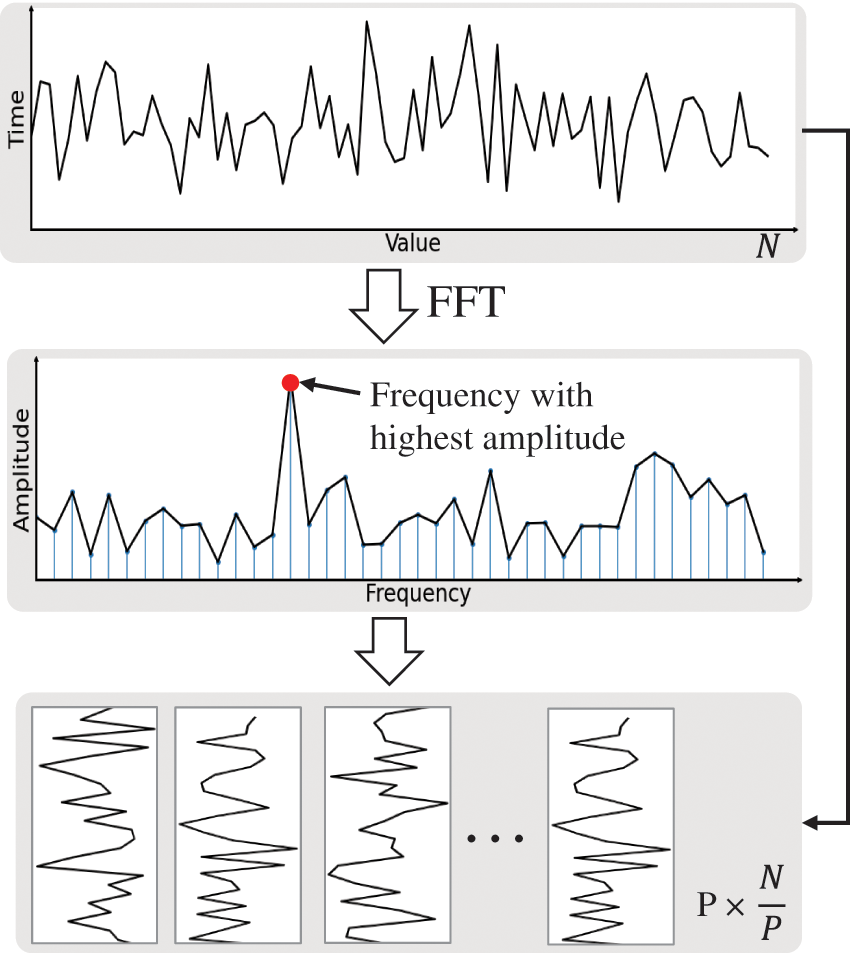
Figure 2: Conversion of time series from 1D to 2D using FFT

Freqmax=argmax(Amplitude(FFT(X)))(3)

Here, FFT(⋅) denotes the FFT function, and Amplitude(⋅) represents the calculation of amplitude values. Freqmax represents the frequency with the largest amplitude. The period of the time series can be directly obtained as ⌈1Freqmax⌉. Based on the frequency and the period length, the 1D time series can be converted to 2D space by splitting and stacking. Specifically, we split the 1D time series into shorter segments with a length of ⌈1Freqmax⌉, and then stack them in a newly created dimension. For a 1D time series with length N and discovered period P, the converted 2D form has a shape P×PN. This process can be summarized as:

A2D=Split_and_Stack(X,Freqmax)(4)

3.4 Cross-Dimension Attentive Feature Fusion

For the 1D representations, we utilize the series and feature mixing strategy to extract abstract high-level patterns. For 2D representations, we employ stacked separable convolutions [57] to learn features. This approach facilitates communication between different periods, making it less vulnerable to complex periodicity properties. After the convolution, the features are flattened into 1D representations, formulated as:

X2D=Flatten(Sep_Conv(A2D))(5)

As features in different dimensions may possess varying levels of representation ability, we introduce an attentive mechanism for feature fusion, depicted in Fig. 3. Three fully connected layers and the sigmoid function are employed for each feature to generate the attention score. These scores are then used to weight the input feature through element-wise multiplication. To break the symmetric structure, one branch further multiplies by a factor of a negative one and adds a positive one. This operation still outputs a value in the range from zero to one, making it compatible with the sigmoid function. This attentive feature fusion process can be formally denoted as:

Figure 3: Feature fusion scheme in the proposed method (FC and σ means fully connected layer and sigmoid function, respectively)

X(l+1)=σ(F(X1Dl))⊗X1Dl+(σ(F(X2Dl)∗(−1)+1)⊗X2Dl(6)

where l indicates the block number, F, σ and ⊗ represent fully connected layers, sigmoid function and element-wise multiplication, respectively.

To provide an intuitive understanding of the Eq. (6), we transform it into the following equivalent form. In this form, the output of the sigmoid activation can be viewed as a gate that controls the information flow of a feature branch.

X(l+1)=σ(F(X1Dl))⊗X1Dl+(1−σ(F(X2Dl))⊗X2Dl(7)

The fused features X(l+1) serve as the input to the next 1D and 2D blocks. The output of the final feature fusion block is then mapped by a fully connected layer, computed as O∗=FullyConnected(XL) and can be regarded as the reconstruction of the input time series X0. The loss function can then be constructed as:

L=1N∑i=1N(X0(i)−O∗(i))2(8)

where N denotes the number of time series segments.

The algorithm table is provided in Algorithm 1, which delineates the detailed algorithm steps for training the CAFFN model. We initialize the CAFFN model as depicted in Fig. 1, and proceed with the optimization of parameters achieved through the minimization of the loss function defined in Eq. (8).

4  Experiments

4.1 Datasets and Metrics

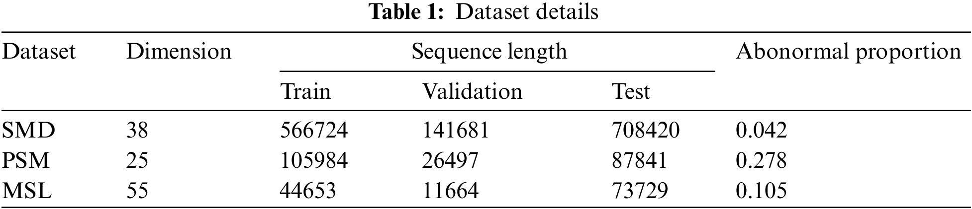
We assess the performance of CAFFN on three widely used anomaly detection benchmarks obtained from real-world applications. (1) SMD (Server Machine Dataset) [51] is a 5-week-long dataset with 38 dimensions collected from an Internet company. (2) MSL (Mars Science Laboratory rover) [58] is with dimensions of 55, and was collected by NASA. (3) SMAP (Soil Moisture Active Passive satellite) [58] is a public dataset from NASA with the dimension of 25. Following the setting in previous studies, the dataset is split into consecutive non-overlapping segments in a pre-processing step. Abnormalities in a segment are considered detected if a single abnormal time point in that segment is identified. More details of the dataset can be found in Table 1. As a commonly adopted metric for unsupervised point-wise representation learning scenarios, the reconstruction error is considered a natural anomaly criterion in experiments. Additionally, various criteria, including Precision, Recall, and F1-score metrics, are adopted to evaluate performance comprehensively.

4.2 Implementation Details

To ensure a fair comparison, we adhere to the settings in previous studies [52]. The non-overlapping windows size is set to 100 for all datasets, and a time point is labeled as an anomaly if the anomaly score is larger than a threshold determined by the statistics of the training set. We empirically found the optimal architectural setting based on grid search and GPU memory constraints. The setting that achieved the best result on the validation set is selected for experimental comparison on the test set. Specifically, the feature blocks are stacked three times for all datasets (L = 3). The sizes of hidden layers in series mixing and feature mixing are set to 32 and 64, respectively. Regarding the CAFFN model, the first FC layers in the attentive fusion module map the input to a feature with half of the input’s length. The second FC layer does not change the dimensionality, and the third FC layer maps the feature back to the space whose dimensionality is the same as the module input. Adam, with default settings, is used for parameter optimization with a batch size of 128, and the training process is stopped within 10 epochs. All experiments are implemented using Pytorch and run on a computer equipped with an NVIDIA RTX3090 GPU.

4.3 Quantitative Results

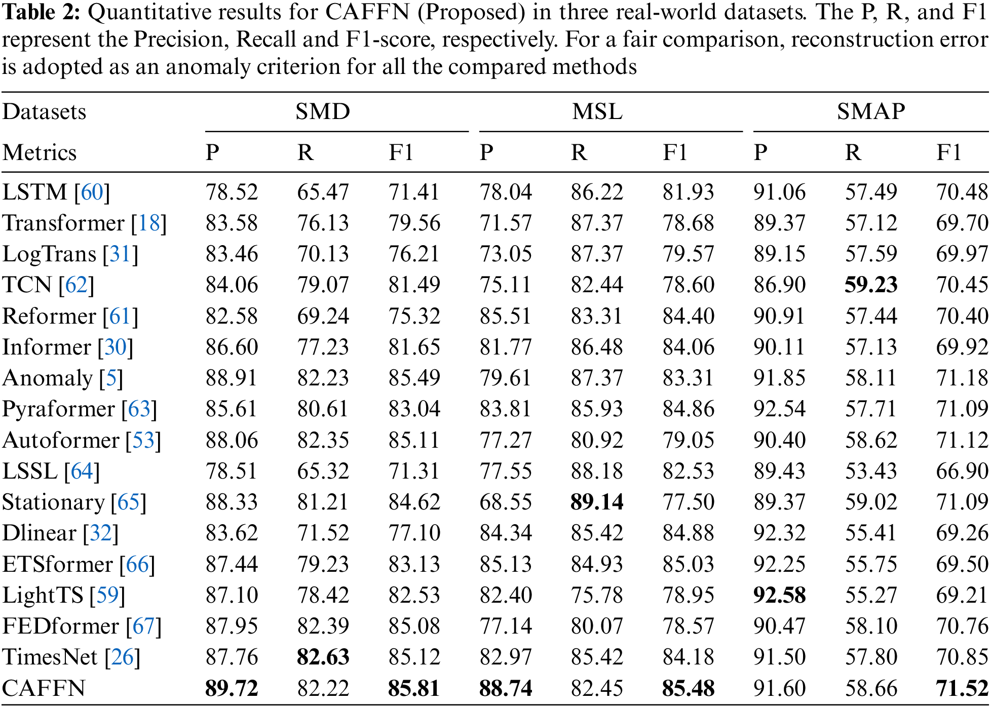
The performance of the proposed CAFFN model on time series anomaly detection datasets is shown in Table 2. Additionally, we made a comparison to highly related competitive methods. In particular, MLP-based [32,59], RNN-based [60], CNN-based [26,61], and many other Transformer-based time series anomaly detection are considered. As seen, the widely used F1-score metric of the proposedCAFFN model on SMD, MSL, and SMAP are 85.81%, 85.48% and 71.52%, respectively. This indicates the proposed CAFFN can outperform RNN-based methods like LSTM by a large margin, primarily attributed to its capability to capture long-term dependencies. Moreover, the performance of the proposed CAFFN model is superior to many other Transformer based methods, showcasing its superiority in modeling the complex feature of time series. This aligns with previous studies that have surprisingly found that even simple linear models can outperform Transformer-based models [32]. The slightly worse performance achieved by TimeNet [26] indicates that capturing features in 2D space can provide strong results. The proposed CAFFN model learns features in both 1D and 2D spaces, which could be the main reason for its superior performance. Compared to existing deep learning-based time series anomaly detection methods, the proposed CAFFN model employs a well-designed feature extraction block, which can provide the stronger capability to capture the spatial and temporal features of time series data.

4.4 Qualitative Results

The reconstruction errors on the SMD training set and validation set during model training are recorded and presented in Fig. 4. It can be observed that the error decreases on both the training and validation sets, validating the capability of CAFFN in modeling time series data.

Figure 4: Reconstruction errors on SMD dataset

The detection results for some test segments in MSL are illustrated in Figs. 5 and 6. It is evident that the anomaly score significantly increases when the segments of the time series contain anomalous events, indicating that abnormal patterns are reconstructed with a substantial error. Although the time steps of annotated anomalies and predicted ones are not precisely aligned, common practice usually allows for the detection of anomalies in a reasonably wide window. Therefore, the detection results serve as an accurate indicator to localize the time points of anomalies, as shown in the figures for most of the time.

Figure 5: Anomaly score and ground-truth on MSL test set from time step 45985 to 46125 (values of ground truth are adaptively scaled for better visualization)

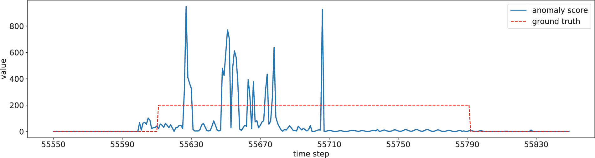
Figure 6: Anomaly score and ground-truth on MSL test set from time step 55550 to 55830 (values of ground-truth are adaptively scaled for better visualization)

4.5 Ablation Study

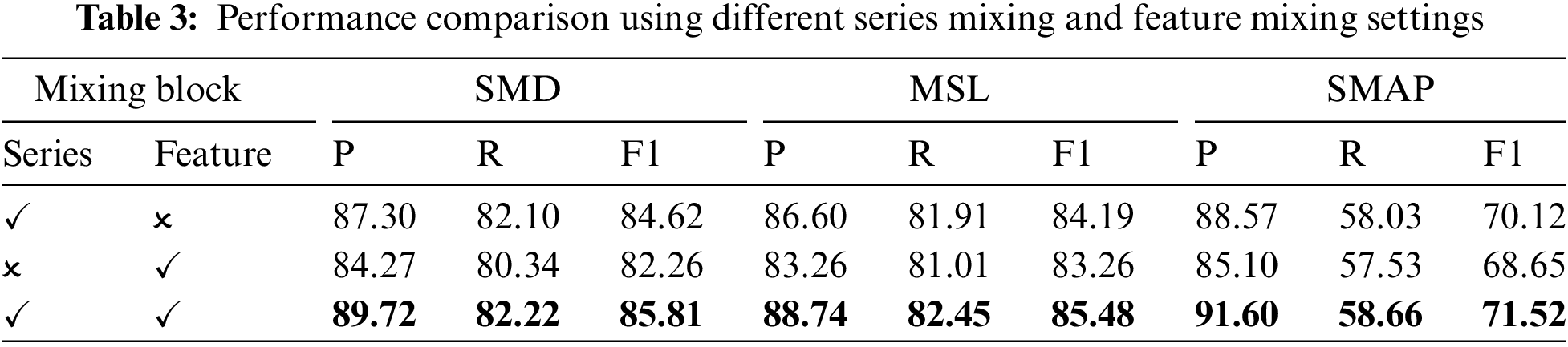
In this subsection, we evaluate the effectiveness of each component in the proposed CAFFN model. Firstly, different settings of the mixing block are investigated by disabling either the series mixing block or feature mixing block. Specifically, we can remove the feature mixing part from the mixing 1D block without affecting the output shape. Additionally, by directly feeding the input to the feature mixing module and removing the series mixing module, we can also obtain a valid mixing 1D block, as shown in Fig. 1. The results are shown in Table 3.

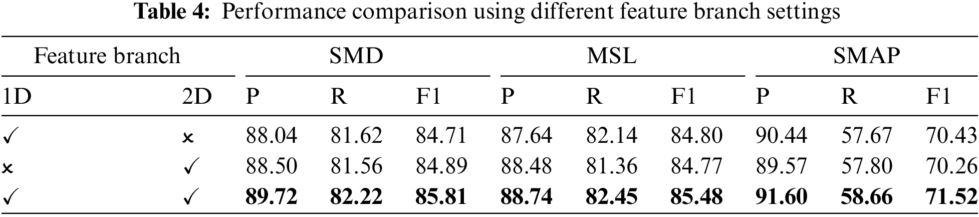
Additionally, the feature branch in the proposed CAFFN model is investigated similarly. We first disable the branch that uses a 2D block while keeping the branch that uses a 1D block valid. In this setting, the proposed model lacks the capability of capturing 2D features, and cross-dimension attentive feature fusion is not needed. The performance of this configuration is shown in Table 4, where a considerable performance degradation can be observed in the first line. Next, we enable the branch that uses 2D block but disable the branch that uses 1D block. In this case, the model is incapable of learning 1D features, and the results are shown in the second line in Table 4. It can be seen that the performance is slightly better than in the previous situation, verifying the advantage of employing FFT for discovering 2D structures in time series. The performance further improves when both branches are enabled, as indicated by the final line in Table 4, where features from 1D and 2D spaces are fused for anomaly detection. Therefore, the two-branch structure is necessary for obtaining promising performance.

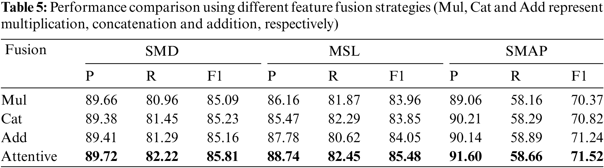
To validate the effectiveness of the attentive feature fusion mechanism in the proposed method, we compare it to other alternative feature fusion schemes, including multiplication, concatenation, and addition. The results of different feature fusion strategies are shown in Table 5. It can be observed that all three settings provide a slightly worse performance than the proposed attentive mechanism, verifying the merits of the CAFFN model.

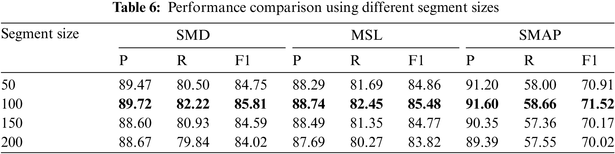
We further investigate the impact of different segment sizes on the performance, and the results are shown in Table 6. It indicates that the segment size has a slight influence on the performance, and setting the segment size to 100 can achieve promising results.

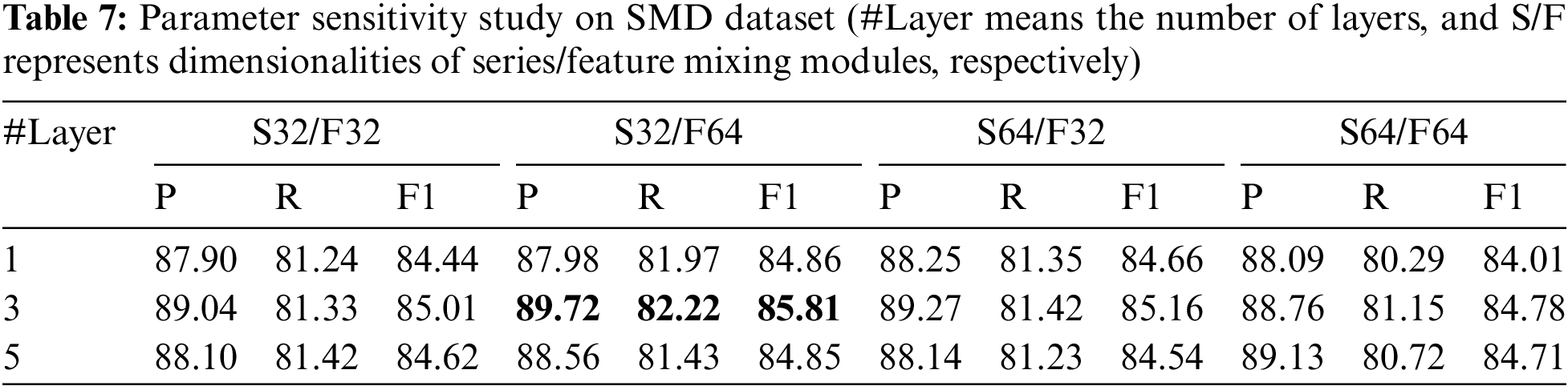
We also investigated the parameter sensitivity of the proposed CAFFN model on the SMD dataset. The results are presented in Table 7. It is evident that the proposed model yields favorable outcomes when configured with a three-layer structure, along with series and feature mixing blocks set to dimensionalities of 32 and 64, respectively.

5  Conclusion

This study proposes a cross-dimension attentive feature fusion network for time series anomaly detection. As a reconstruction-based time series anomaly detection method, we introduced a series and feature mixing block to learn representation in 1D space. Additionally, we adopted a fast Fourier transform to convert the time series into 2D space for learning 2D representations. Furthermore, a cross-dimension attentive feature fusion mechanism was designed to effectively utilize the 1D and 2D features, adaptively integrating features across different dimensions for anomaly detection. Experiments on real-world time series datasets demonstrated that CAFFN outperforms other competing baselines. Moreover, the ablation study confirmed the effectiveness of the feature learning module and the feature fusion mechanism. Future investigation directions include exploring signal processing techniques and generative models for data and feature augmentation.

Acknowledgement: The authors wish to express their appreciation to the reviewers for their helpful suggestions which greatly improved the presentation of this paper.

Funding Statement: This work was supported in part by the National Natural Science Foundation of China (Grants 62376172, 62006163, 62376043), in part by the National Postdoctoral Program for Innovative Talents (Grant BX20200226) and in part by Sichuan Science and Technology Planning Project (Grants 2022YFSY0047,2022YFQ0014, 2023ZYD0143, 2022YFH0021, 2023YFQ0020, 24QYCX0354, 24NSFTD0025).

Author Contributions: The authors confirm contribution to the paper as follows: study conception and design: Rui Wang, Yao Zhou, Dezhong Peng; data collection: Peng Chen; analysis and interpretation of results: Guangchun Luo; draft manuscript preparation: Rui Wang. All authors reviewed the results and approved the final version of the manuscript.

Availability of Data and Materials: The data used in this article are freely available in the mentioned references.

Conflicts of Interest: The authors declare that they have no conflicts of interest to report regarding the present study.

References

1. Geiger, A., Liu, D., Alnegheimish, S., Cuesta-Infante, A., Veeramachaneni, K. (2020). TadGAN: Time series anomaly detection using generative adversarial networks. Proceedings of 2020 IEEE International Conference on Big Data, pp. 33–43. Atlanta, GA, USA. [Google Scholar]

2. Giannoulis, M., Harris, A., Barra, V. (2023). DITAN: A deep-learning domain agnostic framework for detection and interpretation of temporally-based multivariate anomalies. Pattern Recognition, 143, 109814. [Google Scholar]

3. Zeng, F., Chen, M., Qian, C., Wang, Y., Zhou, Y. et al. (2023). Multivariate time series anomaly detection with adversarial transformer architecture in the Internet of Things. Future Generation Computer Systems, 144, 244–255. [Google Scholar]

4. Jhin, S. Y., Lee, J., Park, N. (2023). Precursor-of-anomaly detection for irregular time series. Proceedings of the 29th ACM SIGKDD Conference on Knowledge Discovery and Data Mining, pp. 917–929. Long Beach, CA, USA. [Google Scholar]

5. Xu, J., Wu, H., Wang, J., Long, M. (2021). Anomaly transformer: Time series anomaly detection with association discrepancy. Proceedings of the International Conference on Learning Representations. https://doi.org/10.48550/arXiv.2110.02642 [Google Scholar] [CrossRef]

6. Chen, P., Liu, H., Xin, R., Carval, T., Zhao, J. et al. (2022). Effectively detecting operational anomalies in large-scale IoT data infrastructures by using a gan-based predictive model. The Computer Journal, 65(11), 2909–2925. [Google Scholar]

7. Qadri, Y. A., Nauman, A., Zikria, Y. B., Vasilakos, A. V., Kim, S. W. (2020). The future of healthcare Internet of Things: A survey of emerging technologies. IEEE Communications Surveys & Tutorials, 22(2), 1121–1167. [Google Scholar]

8. Ding, Y., Huang, P., Liang, H., Yuan, F., Wang, H. (2023). Output regeneration defense against membership inference attacks for protecting data privacy. International Journal of Web Information Systems, 19(2), 61–79. [Google Scholar]

9. Xing, M., Ding, W., Zhang, T., Li, H. (2023). STCGCN: A spatio-temporal complete graph convolutional network for remaining useful life prediction of power transformer. International Journal of Web Information Systems, 19(2), 102–117. [Google Scholar]

10. Wu, Q., Xi, C., Ding, L., Wei, C., Ren, H. et al. (2016). Classification of EMG signals by BFA-optimized GSVCM for diagnosis of fatigue status. IEEE Transactions on Automation Science and Engineering, 14(2), 915–930. [Google Scholar]

11. Assous, S., Boashash, B. (2012). Evaluation of the modified s-transform for time-frequency synchrony analysis and source localisation. EURASIP Journal on Advances in Signal Processing, 49(1), 1–18. [Google Scholar]

12. Cui, L. F., Zhang, Q. Z., Shi, Y., Yang, L. M., Wang, Y. X. et al. (2023). A method for satellite time series anomaly detection based on fast-DTW and improved-KNN. Chinese Journal of Aeronautics, 36(2), 149–159. [Google Scholar]

13. Anton, S. D. D., Sinha, S., Schotten, H. D. (2019). Anomaly-based intrusion detection in industrial data with svm and random forests. Proceedings of 2019 International Conference on Software, Telecommunications and Computer Networks (SoftCOM), pp. 1–6. Split, Croatia. [Google Scholar]

14. Gao, H., Wu, Y., Xu, Y., Li, R., Jiang, Z. (2023). Neural collaborative learning for user preference discovery from biased behavior sequences. IEEE Transactions on Computational Social Systems. https://doi.org/10.1109/TCSS.2023.3268682 [Google Scholar] [CrossRef]

15. Gao, H., Wang, X., Wei, W., Al-Dulaimi, A., Xu, Y. (2023). Com-DDPG: Task offloading based on multiagent reinforcement learning for information-communication-enhanced mobile edge computing in the internet of vehicles. IEEE Transactions on Vehicular Technology, Early Access. [Google Scholar]

16. Dosovitskiy, A., Beyer, L., Kolesnikov, A., Weissenborn, D., Zhai, X. et al. (2021). An image is worth 16 × 16 words: Transformers for image recognition at scale. Proceedings of the International Conference on Learning Representations. https://doi.org/10.48550/arXiv.2010.11929 [Google Scholar] [CrossRef]

17. Kim, S., Gholami, A., Shaw, A., Lee, N., Mangalam, K. et al. (2022). Squeezeformer: An efficient transformer for automatic speech recognition. Proceedings of Advances in Neural Information Processing Systems, pp. 9361–9373. New Orleans, LA, USA. [Google Scholar]

18. Vaswani, A., Shazeer, N., Parmar, N., Uszkoreit, J., Jones, L. et al. (2017). Attention is all you need. Proceedings of Advances in Neural Information Processing Systems, pp. 5998–6008. Long Beach, CA, USA. [Google Scholar]

19. Li, G., Jung, J. J. (2022). Deep learning for anomaly detection in multivariate time series: Approaches, applications, and challenges. Information Fusion, 91, 93–102. [Google Scholar]

20. Gong, W., Wang, Y., Zhang, M., Mihankhah, E., Chen, H. et al. (2021). A fast anomaly diagnosis approach based on modified cnn and multisensor data fusion. IEEE Transactions on Industrial Electronics, 69(12), 13636–13646. [Google Scholar]

21. Yin, C., Zhang, S., Wang, J., Xiong, N. N. (2020). Anomaly detection based on convolutional recurrent autoencoder for IoT time series. IEEE Transactions on Systems, Man, and Cybernetics: Systems, 52(1), 112–122. [Google Scholar]

22. Liu, J., Wu, Z., Liu, J., Zou, Y. (2022). Cost research of Internet of Things service architecture for random mobile users based on edge computing. International Journal of Web Information Systems, 18(4), 217–235. [Google Scholar]

23. Canizo, M., Triguero, I., Conde, A., Onieva, E. (2019). Multi-head CNN–RNN for multi-time series anomaly detection: An industrial case study. Neurocomputing, 363, 246–260. [Google Scholar]

24. Liu, S., Zhou, B., Ding, Q., Hooi, B., Zhang, Z. et al. (2022). Time series anomaly detection with adversarial reconstruction networks. IEEE Transactions on Knowledge and Data Engineering, 35(4), 4293–4306. [Google Scholar]

25. Santhosh, K. K., Dogra, D. P., Roy, P. P., Mitra, A. (2021). Vehicular trajectory classification and traffic anomaly detection in videos using a hybrid CNN-VAE architecture. IEEE Transactions on Intelligent Transportation Systems, 23(8), 11891–11902. [Google Scholar]

26. Wu, H., Hu, T., Liu, Y., Zhou, H., Wang, J. et al. (2023). TimesNet: Temporal 2D-variation modeling for general time series analysis. Proceedings of the International Conference on Learning Representations, Kigali, Rwanda. [Google Scholar]

27. Gao, H., Fang, D., Xiao, J., Hussain, W., Kim, J. Y. (2023). CAMRL: A joint method of channel attention and multidimensional regression loss for 3D object detection in automated vehicles. IEEE Transactions on Intelligent Transportation Systems, 24(8), 8831–8845. [Google Scholar]

28. Liu, Z., Lin, Y., Cao, Y., Hu, H., Wei, Y. et al. (2021). Swin transformer: Hierarchical vision transformer using shifted windows. Proceedings of the IEEE International Conference on Computer Vision, pp. 10012–10022. Montreal, QC, Canada. [Google Scholar]

29. Li, Y., Peng, X., Zhang, J., Li, Z., Wen, M. (2023). DCT-GAN: Dilated convolutional transformer-based gan for time series anomaly detection. IEEE Transactions on Knowledge and Data Engineering, 3632–3644. [Google Scholar]

30. Zhou, H., Zhang, S., Peng, J., Zhang, S., Li, J. et al. (2021). Informer: Beyond efficient transformer for long sequence time-series forecasting. Proceedings of the AAAI Conference on Artificial Intelligence, pp. 11106–11115. [Google Scholar]

31. Li, S., Jin, X., Xuan, Y., Zhou, X., Chen, W. et al. (2019). Enhancing the locality and breaking the memory bottleneck of transformer on time series forecasting. Proceedings of Advances in Neural Information Processing Systems, pp. 5244–5254. Vancouver, BC, Canada. [Google Scholar]

32. Zeng, A., Chen, M., Zhang, L., Xu, Q. (2023). Are transformers effective for time series forecasting?. Proceedings of the AAAI Conference on Artificial Intelligence, pp. 11121–11128. Washington DC, USA. [Google Scholar]

33. Grubbs, F. E. (1969). Procedures for detecting outlying observations in samples. Technometrics, 11(1), 1–21. [Google Scholar]

34. Golan, I., El-Yaniv, R. (2018). Deep anomaly detection using geometric transformations. Proceedings of Advances in Neural Information Processing Systems, pp. 31. Montréal, Canada. [Google Scholar]

35. Yuan, Z., Chen, B., Liu, J., Chen, H., Peng, D. et al. (2023). Anomaly detection based on weighted fuzzy-rough density. Applied Soft Computing, 134, 109995. [Google Scholar]

36. Chen, B., Li, Y., Peng, D., Chen, H., Yuan, Z. (2024). Fusing multi-scale fuzzy information to detect outliers. Information Fusion, 103, 102133. [Google Scholar]

37. Wang, S., Zeng, Y., Liu, X., Zhu, E., Yin, J. et al. (2019). Effective end-to-end unsupervised outlier detection via inlier priority of discriminative network. Proceedings of Advances in Neural Information Processing Systems, pp. 32. Vancouver, BC, Canada. [Google Scholar]

38. Box, G. E., Jenkins, G. M., Reinsel, G. C., Ljung, G. M. (2015). Time series analysis: Forecasting and control. USA: John Wiley and Sons Inc. [Google Scholar]

39. Gardner Jr, E. S. (1985). Exponential smoothing: The state of the art. Journal of Forecasting, 4(1), 1–28. [Google Scholar]

40. Winters, P. R. (1960). Forecasting sales by exponentially weighted moving averages. Management Science, 6(3), 324–342. [Google Scholar]

41. Harvey, A. C. (1990). Forecasting, structural time series models and the Kalman filter. UK: Cambridge University Press. [Google Scholar]

42. Damianou, A., Lawrence, N. D. (2013). Deep gaussian processes. Proceedings of the Sixteenth International Conference on Artificial Intelligence and Statistics, pp. 207–215. Scottsdale, AZ, USA. [Google Scholar]

43. Williams, C., Rasmussen, C. (1995). Gaussian processes for regression. Proceedings of Advances in Neural Information Processing Systems. Denver, CO, USA. [Google Scholar]

44. Cao, L. J., Tay, F. E. H. (2003). Support vector machine with adaptive parameters in financial time series forecasting. IEEE Transactions on Neural Networks, 14(6), 1506–1518. [Google Scholar] [PubMed]

45. Sapankevych, N. I., Sankar, R. (2009). Time series prediction using support vector machines: A survey. IEEE Computational Intelligence Magazine, 4(2), 24–38. [Google Scholar]

46. Ha, T., Dang, T. K. (2022). Inference attacks based on gan in federated learning. International Journal of Web Information Systems, 18(2/3), 117–136. [Google Scholar]

47. Döschl, A., Keller, M. E., Mandl, P. (2021). Performance evaluation of gpu-and cluster-computing for parallelization of compute-intensive tasks. International Journal of Web Information Systems, 17(4), 377–402. [Google Scholar]

48. Cao, X., Guo, Y., Yang, W., Luo, X., Xie, S. (2023). Intrinsic feature extraction for unsupervised domain adaptation. International Journal of Web Information Systems, 5(6), 173–189. [Google Scholar]

49. Ahmad, S., Lavin, A., Purdy, S., Agha, Z. (2017). Unsupervised real-time anomaly detection for streaming data. Neurocomputing, 262, 134–147. [Google Scholar]

50. Yang, W., Liu, C., Jiang, D. (2018). An unsupervised spatiotemporal graphical modeling approach for wind turbine condition monitoring. Renewable Energy, 127, 230–241. [Google Scholar]

51. Su, Y., Zhao, Y., Niu, C., Liu, R., Sun, W. et al. (2019). Robust anomaly detection for multivariate time series through stochastic recurrent neural network. Proceedings of the 25th ACM SIGKDD International Conference on Knowledge Discovery & Data Mining, pp. 2828–2837. Anchorage, Alaska, USA. [Google Scholar]

52. Shen, L., Li, Z., Kwok, J. (2020). Timeseries anomaly detection using temporal hierarchical one-class network. Proceedings of Advances in Neural Information Processing Systems, pp. 13016–13026. Vancouver, Canada. [Google Scholar]

53. Wu, H., Xu, J., Wang, J., Long, M. (2021). Autoformer: Decomposition transformers with auto-correlation for long-term series forecasting. Proceedings of Advances in Neural Information Processing Systems, 34, 22419–22430. [Google Scholar]

54. Tolstikhin, I. O., Houlsby, N., Kolesnikov, A., Beyer, L., Zhai, X. et al. (2021). MLP-Mixer: An all-MLP architecture for vision. Proceedings of Advances in Neural Information Processing Systems, 34, 24261–24272. [Google Scholar]

55. Zhou, B., Liu, S., Hooi, B., Cheng, X., Ye, J. (2019). BeatGAN: Anomalous rhythm detection using adversarially generated time series. Proceedings of the International Joint Conference on Artificial Intelligence, pp. 4433–4439. Macao, China. [Google Scholar]

56. Hendrycks, D., Gimpel, K. (2016). Gaussian error linear units (GELUs). arXiv preprint arXiv:1606.08415. [Google Scholar]

57. Howard, A. G., Zhu, M., Chen, B., Kalenichenko, D., Wang, W. et al. (2017). MobileNets: Efficient convolutional neural networks for mobile vision applications. arXiv preprint arXiv:1704.04861. [Google Scholar]

58. Hundman, K., Constantinou, V., Laporte, C., Colwell, I., Soderstrom, T. (2018). Detecting spacecraft anomalies using lstms and nonparametric dynamic thresholding. Proceedings of the 24th ACM SIGKDD International Conference on Knowledge Discovery & Data Mining, pp. 387–395. London, UK. [Google Scholar]

59. Zhang, T., Zhang, Y., Cao, W., Bian, J., Yi, X. et al. (2022). Less is more: Fast multivariate time series forecasting with light sampling-oriented mlp structures. arXiv preprint arXiv:2207.01186. [Google Scholar]

60. Graves, A., Graves, A. (2012). Long short-term memory. Supervised Sequence Labelling with Recurrent Neural Networks, 385, 37–45. [Google Scholar]

61. Kitaev, N., Kaiser, Ł., Levskaya, A. (2020). Reformer: The efficient transformer. arXiv preprint arXiv: 2001.04451. [Google Scholar]

62. Franceschi, J. Y., Dieuleveut, A., Jaggi, M. (2019). Unsupervised scalable representation learning for multivariate time series. Proceedings of Advances in Neural Information Processing Systems, pp. 4652–4663. Vancouver, BC, Canada. [Google Scholar]

63. Liu, S., Yu, H., Liao, C., Li, J., Lin, W. et al. (2021). Pyraformer: Low-complexity pyramidal attention for long-range time series modeling and forecasting. Proceedings of the International Conference on Learning Representations, Vienna, Austria. [Google Scholar]

64. Gu, A., Goel, K., Ré, C. (2021). Efficiently modeling long sequences with structured state spaces. arXiv preprint arXiv:2111.00396. [Google Scholar]

65. Liu, Y., Wu, H., Wang, J., Long, M. (2022). Non-stationary transformers: Rethinking the stationarity in time series forecasting. Proceedings of Neural Information Processing Systems, New Orleans, LA, USA. [Google Scholar]

66. Woo, G., Liu, C., Sahoo, D., Kumar, A., Hoi, S. (2022). Etsformer: Exponential smoothing transformers for time-series forecasting. arXiv preprint arXiv:2202.01381. [Google Scholar]

67. Zhou, T., Ma, Z., Wen, Q., Wang, X., Sun, L. et al. (2022). Fedformer: Frequency enhanced decomposed transformer for long-term series forecasting. Proceedings of the International Conference on Machine Learning, pp. 27268–27286. Baltimore, Maryland, USA. [Google Scholar]