An Image Fingerprint and Attention Mechanism Based Load Estimation Algorithm for Electric Power System

1  Introduction

With the improvement of people’s living standards, the requirement for power load increases dramatically [1–3]. In order to solve the shortage of the power load, one simple solution is to expand the scale of the power system. However, this method needs a huge investment and does not meet the requirements of carbon peaking and carbon neutrality goals. Since load estimation can give power load requirements in the next time interval, it has received much attention for power generation cost reduction and improving economic benefits [4].

Generally, three main load estimation techniques have been proposed. The first kind of load estimation technique is called the traditional load estimation technique, using the Kalman filter and exponential smoothing model. In [5], three different kinds of filters with time-varying, time-invariant, and steady-state are proposed to estimate the electric load. The simulation results described better estimation performance. In [6], a novel blind Kalman filter is proposed for short-term load estimation by the estimated linear state space model and observation matrices. However, the smoothing coefficient has a great effect on final estimation performance. Optimal smoothing coefficient can lead to better estimation performance [7].

The second kind of load estimation technique is based on time series and regression analysis. In [8], the statistical time series model is proposed for load estimation in a public hospital facility using seasonal auto-regressive integral moving averages. In [9], a multi-level recursive regression analysis is proposed for load estimation. It can be seen that the proposed algorithm has a strong adaptability to the sequential variance of the power system. In [10], the linear, compound-growth and quadratic regression techniques are proposed for load estimation by previous load consumption.

Lastly, the third kind of load estimation technique is based on the machine learning technique. The artificial neural networks (ANN) have been used for electrical load estimation since 1990 [11]. By updating network architecture and connection weights, the ANN can obtain the relationship between the measurements and the actual loads. Back Propagation (BP), as the most common ANN structure, is proposed for load estimation [12]. With the development of machine learning, the support vector machine (SVM) is proposed to solve the regression and classification task [13]. A multistep load forecasting algorithm by phase space reconstruction and SVM is proposed to solve pseudo midterm forecast and divergence of the forecasting error [14]. Experiment results show that the multistep implemented model has more accurate prediction results and stronger robustness. The extreme learning machine (ELM) method now shows better generalization performance than the ANN and SVM methods [15]. The genetic quantum particle swarm optimization and regularized extreme learning machine (RELM) algorithm are also proposed to improve the short-term load forecasting performance [16].

Recently, deep learning, as a better artificial intelligence technique, has been developed to solve many complex pattern recognition problems. It uses multiple processing layers with complex structures or multiple nonlinear transformations to obtain effective feature expression automatically. Thus, many deep learning based load estimation algorithms have been proposed. A multiple wavelet convolutional neural network (CNN) is proposed for load forecasting [17]. As we know, the CNN architecture has a great effect on final load estimation performance. In order to improve the stability and reliability of the prediction model, the Harris hawks optimization approach is proposed to optimize the initial learning rate of long short-term memory recurrent neural networks (RNNs) and the number of hidden-layer units [18].

In this paper, we will continue to study the deep learning based load estimation algorithm. Through the above previous work description in [17,18], many challenges that limit the utilization of the deep learning technique should be solved. First, a new fingerprint construction of the training data is required. As we know, the main advantage of deep learning is that it has better performance for image classification. However, for actual load estimation, most of the measurements are obtained from the deployed sensors. For instance, temperature, humidity and pressure measurements are the one data rather than the image. Thus, without the fingerprint construction, only the data vector is chosen as the input of some existing off-line training. In order to expand the utilization of the deep learning method, the 2-dimension fingerprint construction algorithm should be studied first. Second, a new machine learning framework is required to improve the training performance. Compared with traditional load estimation algorithms, deep learning-based techniques can extract the feature of a fingerprint automatically. However, because of high-dimension representation, these features usually contain some redundancy that should be deleted. Thus, deep learning combined with an attention mechanism is very important for load estimation applications.

In order to solve the above two main problems, a deep learning-based load estimation algorithm using image fingerprints and an attention mechanism is proposed in this paper. The contributions of this paper can be summarized as follows:

(1) In order to satisfy the input requirement for most deep learning networks, an image fingerprint construction algorithm is proposed. The obtained measurement vector is transformed into a data matrix using the cyclic shift at first. Then, in order to obtain a better image description, the cubic spline interpolation is used to expand the matrix dimension. The cubic spline interpolation technique is a trade-off between flexibility and computation speed. Compared with the higher order spline interpolation method, it only requires less computation and storage. Moreover, it is more flexible than the second spline interpolation technique. Next, the linear mapping method is proposed to transform the matrix into the gray image fingerprint. Finally, the gray-color transformation technique is proposed to transform the gray image into a color image. Through the gray-color transformation, it can improve the discernment of image details and achieve image enhancement. Through the proposed image fingerprint construction algorithm, the obtained training data fingerprint can be used for most of deep learning networks.

(2) In order to improve the off-line learning performance, a CNN and attention mechanism based network is proposed for the training process. In particular, the convolutional block attention module (CBAM) proposed in [19] is embedded into the CNN to train the relationship between the image fingerprint and the actual load. Since the CBAM increases the weight of important information and improves the quality of feature representation, it can obtain better training performance for practical application.

(3) An experiment is carried out to evaluate the estimation performance of the proposed algorithm. Based on the actual training data obtained in one community of Jiangsu Province, the proposed algorithm has better load estimation performance than some existing deep learning based approaches in terms of mean absolute error (MAE) and root mean square error (RMSE).

The remainder of this paper is organized as follows. The off-line phase description and the on-line phase description of the proposed algorithm are proposed in Sections 2 and 3, respectively. Experiment and performance analysis are illustrated in Section 4 and the conclusion is given in Section 5.

2  Off-Line Phase Description of the Proposed Algorithm

According to the block diagram shown in Fig. 1, the off-line phase of the proposed algorithm contains four main steps: (1) Measurement data preprocessing (2) Training data matrix construction (3) Training image fingerprint construction and (4) CNN and attention mechanism based off-line learning.

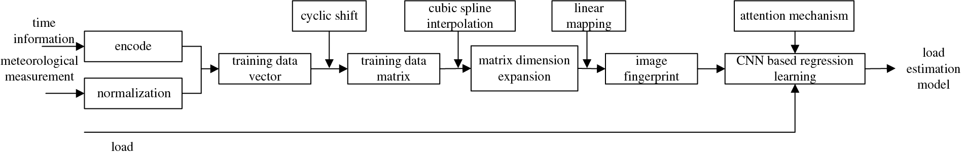
Figure 1: The block diagram of the off-line phase for the proposed algorithm

After the preprocessing of the time information and meteorological measurements, the training data vector is obtained at first. Then, the training data vector is transformed into a matrix form by the cyclic shift. Moreover, the dimension of the data matrix is also expanded using cubic spline interpolation. Next, the linear mapping approach is used to transform the data matrix into an image fingerprint. Lastly, off-line learning by CNN and an attention mechanism are proposed to obtain the load estimation model. In the following, each step will be described in detail.

2.1 Measurement Data Preprocessing

For data collection, the meteorological sensor is used to measure the weather data. At the same time, the corresponding time information and actual load are also recorded. Based on the above-obtained measurements, the data preprocessing is described as follows.

At first, the time information is processed by encoding. Through the correlation analysis between the time and load, we found that the time burden of peak load is usually at 18:00–24:00. While the time burden of the bottom load is close to 0:00–6:00. So, from the proposed encoding process shown in Fig. 2, the time of each day is divided into four time regions: 0:00–6:00, 6:00–12:00, 12:00–18:00 and 18:00–24:00. Each time region is encoded with one integer. Moreover, the month information is encoded from 1 to 12 in turn.

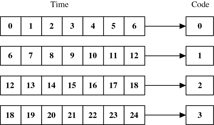
Figure 2: The description of time information coding processing

For another, since the meteorological measurements are obtained from different sensors, the data range of these measurements is different. In order to mitigate data range influence, in this step, a max-min normalized method is used to increase the data comparability for the measurements. For ith kind information, the process of nth measurement is described as [20]:

xi,n′=xi,n−xi,minxi,max−xi,min(1)

where xi,n,xi,n′ is the original data and normalized result xi,max,xi,min is the maximum and minimum of the data information.

Through the normalized data processing, all the meteorological information and time information are with the interval [0, 1].

After data combination, the nth training data vector can be described as:

xn=[x1,n′,⋯,xm,n′,tn′,dn′](2)

where tn′ and dn′ describe the normalized time information and month information, respectively, m is the number of meteorological information.

2.2 Training Data Matrix Construction

The aim of this step is to transform the obtained training data vector into a matrix version by cyclic shift and cubic spline interpolation.

First, according to the schematic diagram shown in Fig. 3, the original data matrix construction is described as follows.

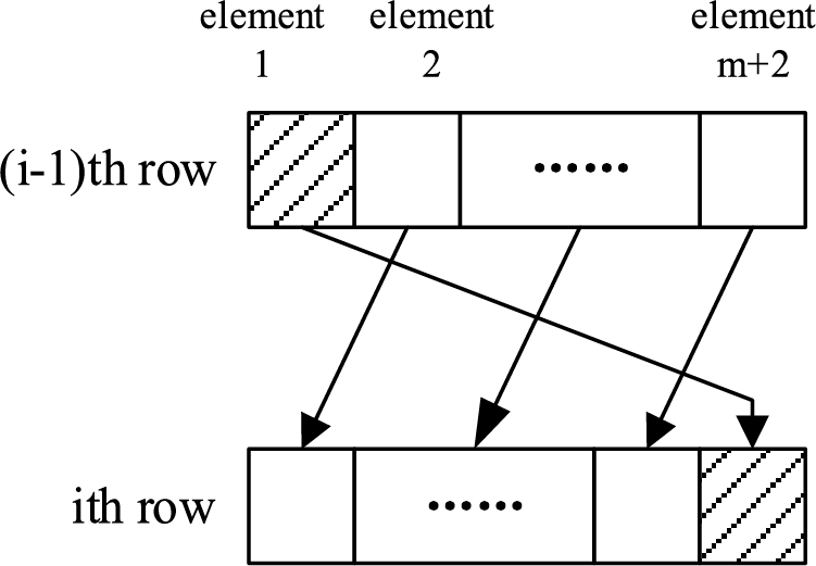
Figure 3: The description of training data matrix construction by cyclic shift

1. The obtained training data vector in Eq. (2) is chosen as the first row of the matrix to be constructed.

2. For ith row (i>1) construction, the first element of (i−1) th row is placed at the end of the ith row at first. Then, other elements are shifted to the left one time accordingly.

For the given row parameter q, the above two steps running (q−1) times. At last, the original training data matrix is obtained.

Next, in order to obtain a better description of the image fingerprint, the cubic spline interpolation is used to expand the dimension of the obtained original data matrix.

The basic idea of cubic spline interpolation is that it divides the known data region into several segments with defined cubic functions. The convergence of the piece-wise function has the properties of 0-order continuity, first-order continuity and second-order continuity [21].

Given n+1 data nodes, the data region can be divided into N intervals, and a cubic function is defined in each interval with n segment functions. The function can be defined as:

Si(x)=ai+bi(x−xi)+ci(x−xi)2+di(x−xi)3     (i=0,⋯,n−1)(3)

From Eq. (3), it can be seen that there are four parameters to be solved: ai, bi, ci and di. Thus, the total number of parameters to be solved is 4n. In order to achieve this solution, the conditions are summarized as follows:

•Condition 1: The given function passes some known points which has n+1 equations.

Si(xi)=yi(i=0,1,⋯,n−2)(4)

•Condition 2: The last value of ith function should be equal to the first value of (i+1)th function which has n−1 equations.

Si(xi+1)=Si+1(xi+1)(i=0,1,⋯,n−2)(5)

•Condition 3: All nodes are first order continuous which has n−1 equations.

Si′(xi+1)=Si+1′(xi+1)(i=0,1,⋯,n−2)(6)

•Condition 4: All nodes are second order continuous which has n−1 equations.

Si″(xi+1)=Si″(xi+1)(i=0,1,⋯,n−2)(7)

•Condition 5: Natural boundary condition.

S0″(x0)=0Sn−1″(xn)=0(8)

From Eqs. (4)–(8), there are 4n equations for parameter solution. Thus, each parameter of ai, bi, ci and di can be obtained.

2.3 Training Image Fingerprint Construction

In this step, the linear mapping method is used for image fingerprint construction.

First, the training data matrix is transformed into a gray image. Assuming the number of gray levels is M, through multiplying M for the data matrix, all the element values belong to the range [0, M]. Thus, the data value at each position of the matrix can be considered as the pixel at the corresponding position of the gray image.

Second, the gray-color transformation method is proposed to form the color image [22,23]. According to the block diagram shown in Fig. 4, the red transform, green transform and blue transform are used to calculate the pixel values of R, G, B. At last, the pixels are mixed to obtain the final color image.

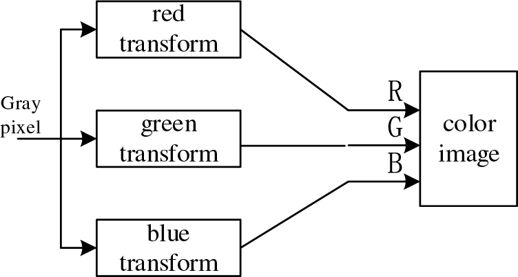
Figure 4: The description of gray-color transformation for color image fingerprint construction

In this paper, these transforms are defined as follows:

R={00≤λ≤2174×λ−510128≤λ≤191255192≤λ≤255(9)

G={4×λ0≤λ≤6325564≤λ≤1911024−4×λ192≤λ≤255(10)

B={2550≤λ≤63510−4×λ64≤λ≤1270128≤λ≤255(11)

where λ is the pix value of the gray image.

Fig. 5 describes the image fingerprint construction result using the proposed image fingerprint construction algorithm. Since there are four meteorological measurements and two numbers of time information, the original size of the data matrix is 6 × 6. In this experiment, after the cubic spline interpolation, the size of the training data matrix is expanded as 24 × 24. Fig. 5a describes the gray image obtained from the linear mapping method. Fig. 5b illustrates the color image by the gray-color transformation method. It can be seen that the proposed algorithm can achieve the color image construction successfully. In order to provide the theoretical support for off-line learning, Fig. 6 shows the image fingerprint results of two different loads. Moreover, some image similarity comparisons are carried out to evaluate the difference of the image fingerprint. The SSIM similarity [24], Cosine similarity [25] and PSNR [26] calculation results are 0.30084, 0.9764 and 28.4343, respectively. Since the two figures are different in theory, it can ensure the efficiency of off-line learning.

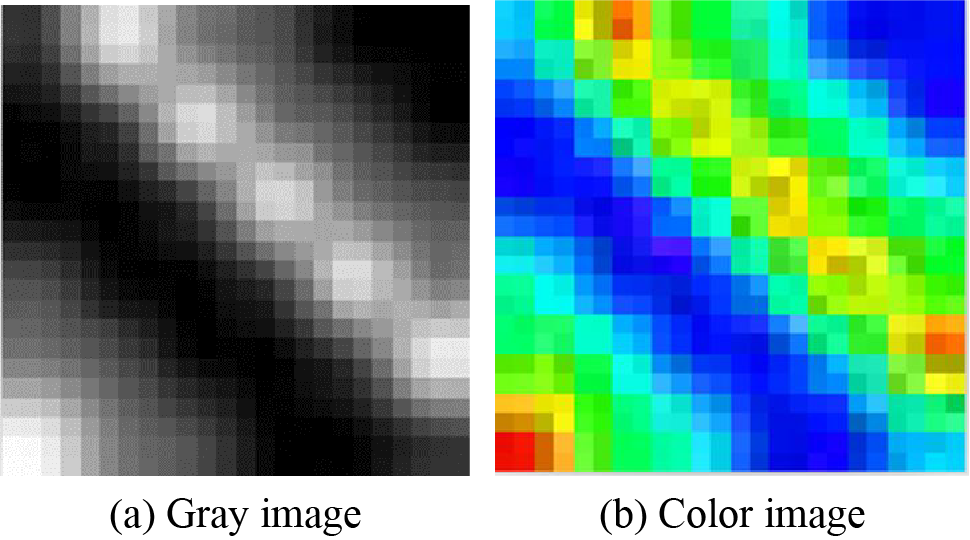
Figure 5: The description of image fingerprint construction result

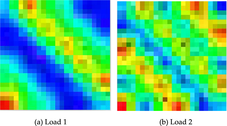
Figure 6: The description of two different image fingerprints

2.4 CNN and Attention Mechanism Based Off-Line Learning

In this step, the CBAM is used to improve CNN’s training performance. According to the block diagram shown in Fig. 7, CBAM combines the channel attention module and spatial attention module in a serial way [27]. In the following, these two attention modules are respectively described in detail at first.

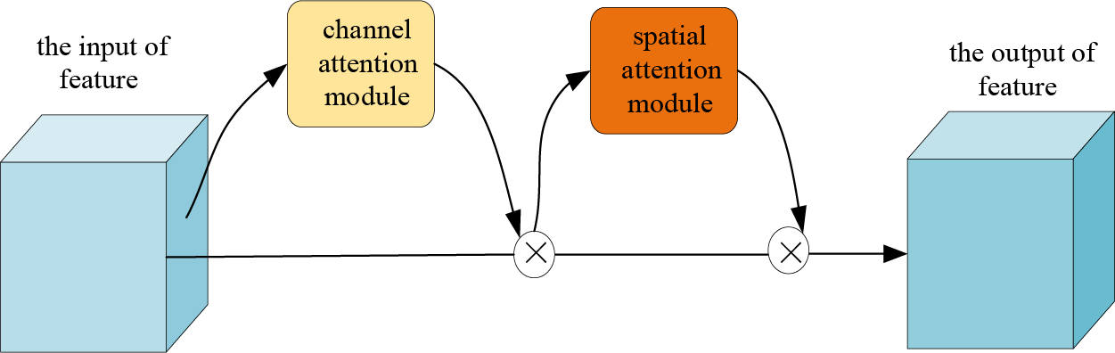
Figure 7: The description of the CBAM structure

Fig. 8 describes the block diagram of the channel attention module where Maxpool and AvgPool describe the max pooling and average pooling, respectively. MLP represents the multi-layer perceptron. δ is sigmoid activation function. Assuming the input is F, the obtained channel attention weights is Mc, and the obtained feature can be written as:

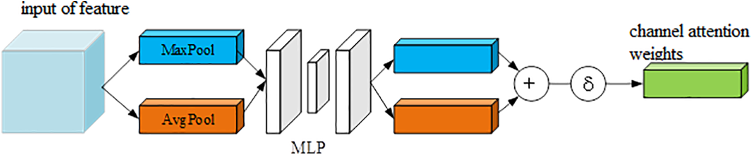
Figure 8: The block diagram of the channel attention module

F′=Mc(F)⊗F=(sigmoid(MLP(AvgPool(F)))+MLP(MaxPool(F)))⊗F(12)

Next, this feature is used as the input for the spatial attention module which is shown in Fig. 9. The process of spatial attention module is described as follows.

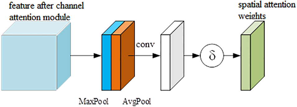
Figure 9: The block diagram of spatial attention module

First, after the maximum pooling and average pooling operations with the spatial dimension, the obtained results are combined in parallel. Then, after convolution and sigmoid activation function process, the spatial attention weight is obtained which is given by:

Ms=Sigmoid(f([AvgPool(F′);MaxPool(F′)]))(13)

When the weight is multiplied by the features input, the final output features can be calculated as:

FL=Ms(F′)⊗F′(14)

Based on the chosen CBAM for feature extraction, the framework of the off-line learning is described in Fig. 10.

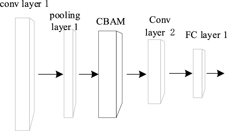
Figure 10: The description of CNN framework for off-line learning

In the proposed network, it contains two convolutional layers, one pooling layer and one fully connected (FC) layer. For the convolutional layer, the size of the convolution kernel is 3 × 3, the activation function is the ReLU function. The number of convolutional kernel for the first and second layer are 32 and 64, respectively. For the pooling layer, the max-pooling approach is chosen with the size of 2 × 2. The padding method is SAME and the stride is 1. The FC layer contains 64 neurons with the ReLU function.

After the feature extraction, the linear activation function is used to achieve the regression learning. The loss function is chosen as the MSE criteria.

Note that in this paper, the size and the number of convolution kernel, the size and the stride of the pooling layer are chosen by the many experiments. First, based on a number of predefined parameters, training processing is carried out to get multiple load estimation models. By the performance evaluation with test data, the model with the best estimation performance is selected. The above CNN network parameters corresponding to this model are the chosen parameters in this paper. How to determine the optimal parameters above will be our research work in the future.

3  On-Line Phase Description of the Proposed Algorithm

In the on-line phase, the load can be estimated based on the obtained meteorological measurements and the given time information. First, the measurement preprocessing is used for the obtained measurement vector. Based on the normalized time information and meteorological measurements, the final on-line fingerprint vector can be obtained with Eq. (2). Second, the fingerprint vector is transformed into the matrix version using the cyclic shift shown in Fig. 3. Then, using Eqs. (3)–(8), the cubic spline interpolation is used to expand the dimension of the on-line fingerprint matrix. Third, based on the fingerprint matrix, the linear mapping approach is used to form the gray image fingerprint. Then, the gray-color transformation approach is used for color image fingerprint construction by Eqs. (9)–(11). At last, based on the color image fingerprint, the load can be estimated with the learned network shown in Fig. 10.

4  Experiment and Performance Description

In this section, the experiment is carried out in the community of Jiangsu Province. The temperature, pressure, wind speed, and humidity, four different types of meteorological information, are measured from sensors at some specific times. Moreover, the actual load information at this time is also recorded. During the day, 16 measurements of data were collected per hour. The time duration of measurement collection is from 2015 to 2017. The measurements collected in 2015 and 2016 are chosen as the training data set. The measurements collected in 2017 are used for algorithm evaluation.

The computer with AMD Ryzen 75800 H CPU and 16 GB memory is used for the training process. The machine learning platform is TensorFlow2.1.0 Python3.9. For off-line training, the Adam optimizer is used with a learning rate is 0.001. The batch size and the number of epochs are 64 and 50, respectively. The parameters of validation_split and verbose are set to 0.1 and 2.

4.1 Performance Description of the Proposed Algorithm

First, the off-line training performance is described. Fig. 11 describes the loss with different epochs. It can be seen that when the epoch increases, the loss of the training data set decreases. When the epoch is chosen as 50, the loss is not changed dramatically. Thus, the convergence of off-line training is achieved under this condition and the obtained load estimation model is used for the following performance evaluation.

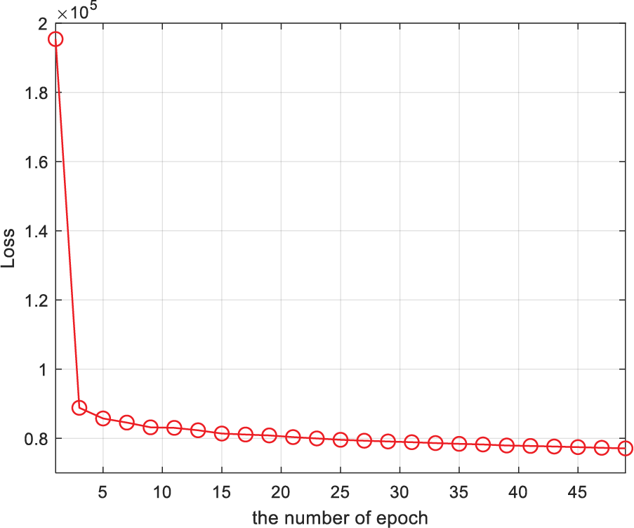
Figure 11: The description of loss for the off-line training

Second, the load estimation performance of the proposed algorithm is described. Fig. 12 describes the load estimation performance with different training numbers. It can be seen that when the training number is 10000, the estimated results are closer to the actual load. Better accurate load estimation can be obtained with more training data. In order to show the performance description clearly, Taking and mean absolute error (MAE), root mean square error (RMSE), mean absolute error percentage (MAPE) and determinate coefficient (R2) as an example, Figs. 13 and 14 describe the above statistical estimation error index for different numbers of training data. When the training number is 10000, it can be seen that the MAE, RMSE, MAPE and R2 are 177.757, 240.1553, 0.1479 and 0.6571, respectively. Based on this statistical index, it can be concluded that the proposed algorithm is suitable for practical application. Compared with the estimation performance with training number 5000, the MAE and RMSE decreased 133.2342 and 138.9417, respectively. Thus, the estimation performance improves dramatically.

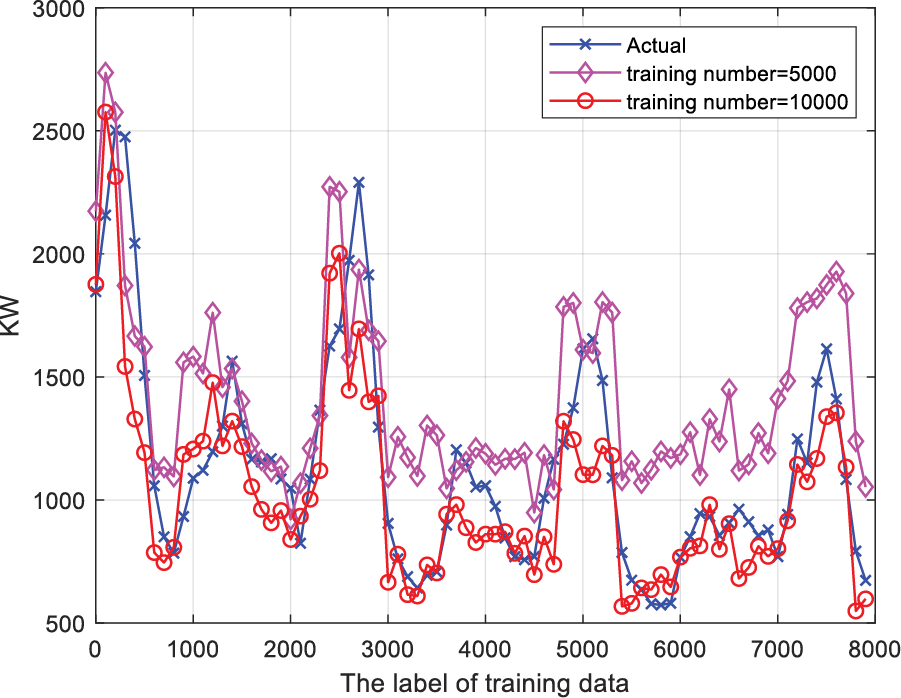
Figure 12: The description of the load estimation performance

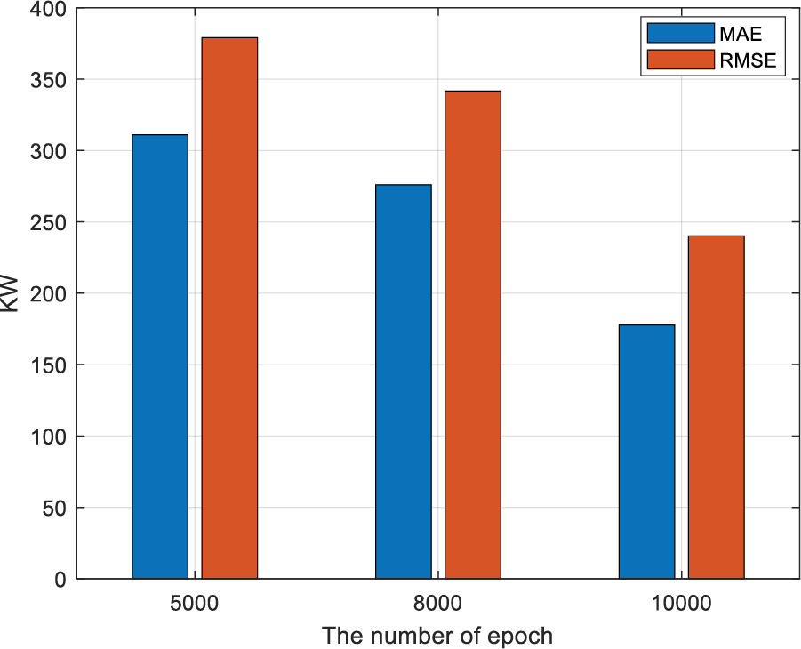
Figure 13: MAE and RMSE description of the proposed algorithm

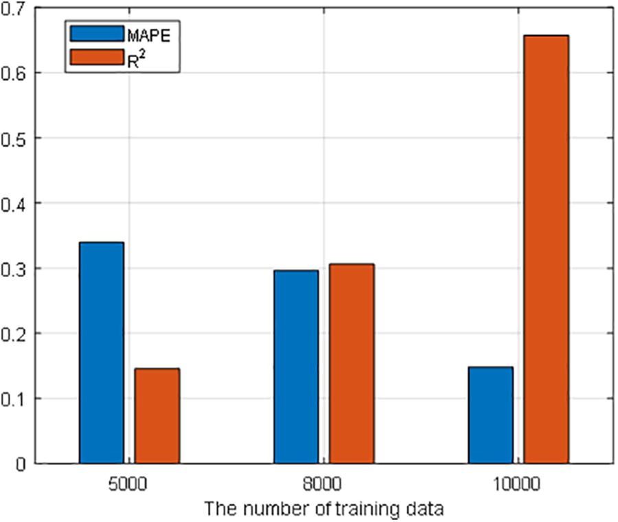
Figure 14: MAPE and R2 description of the proposed algorithm

4.2 Algorithm Performance Comparison

In this section, the algorithm comparison is carried out. Since SVM based method [13], CNN based method [28] and LSTM based method [29] are proposed for load estimation, in this paper, the SVM method, CNN method and LSTM method are straightly chosen for load estimation performance comparison. Taking the training number 10000 as an example, Fig. 15 describes the load estimation for different algorithms. From the experiment results, it can be seen that the distance between the actual load and the estimated load with the SVM method is the largest among these four methods. The estimated error of the proposed algorithm is the smallest. In order to show the performance comparison clearly, Fig. 16 describes the MAE and RMSE for different algorithms. It can be seen that the MAE of the SVM method, CNN method, LSTM method, and the proposed algorithm are 386.9044, 195.0721, 217.3394 and 177.757, respectively. Compared with the SVM method, CNN method and LSTM method, the MAE decreased 209.1474, 17.3151 and 39.5824, respectively. Thus, the proposed algorithm has the best estimation performance among all the methods.

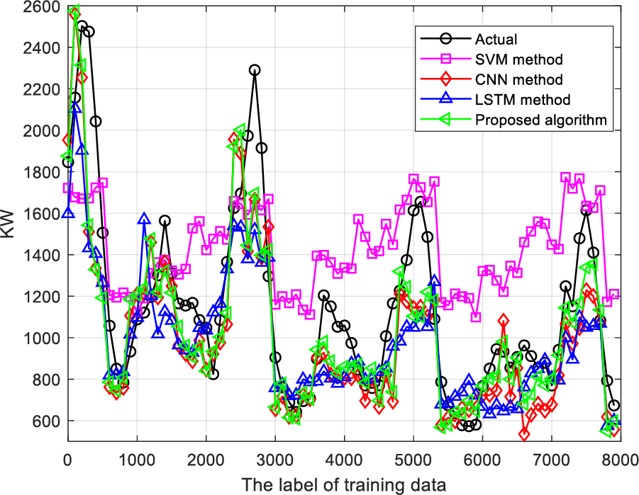
Figure 15: The performance of load estimation for different algorithms

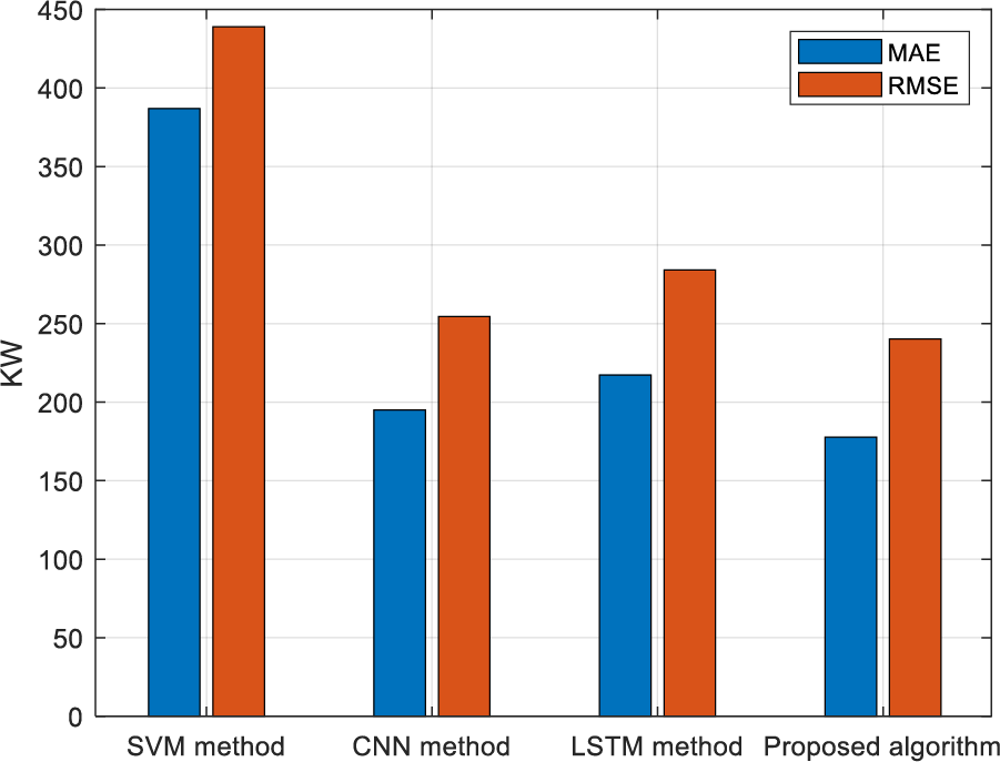
Figure 16: MAE and RMSE comparison

5  Conclusions

In this article, an image fingerprint and attention mechanism based load estimation algorithm is proposed. First, a new training data image fingerprint construction technique is proposed. The cyclic shift and cubic spline interpolation methods are used to build the original training data matrix and expand the matrix dimension, respectively. The linear mapping and gray-color transformation methods are used to form the color image fingerprint. Second, a new machine learning-based training framework is proposed for load estimation by the CNN and CBAM attention mechanism. At last, some experiments are carried out to evaluate the estimation performance. It can be seen that the proposed algorithm performs better than other methods. In the future, we will study the ablation technique to improve the efficiency of the training framework for load estimation.

Acknowledgement: The authors would like to thank the editors and reviewers for their review and recommendations.

Funding Statement: The authors received no specific funding for this study.

Author Contributions: The authors confirm contribution to the paper as follows: study conception and design: Qing Zhu; data collection: Linlin Gu; analysis and interpretation of results: Qing Zhu, Huijie Lin; draft manuscript preparation: Qing Zhu. All authors reviewed the results and approved the final version of the manuscript.

Availability of Data and Materials: Data will be made available on request.

Conflicts of Interest: The authors declare that they have no conflicts of interest to report regarding the present study.

References

1. Chen, C., Su, C., Teng, J. (2020). Electrical load analysis for shipboard power systems using load survey data. IEEE Transactions on Industry Applications, 56(2), 1180–1189. [Google Scholar]

2. Wang, B., Zhao, D., Dehghanian, P., Tian, Y., Hong, T. (2020). Aggregated electric vehicle load modeling in large-scale electric power systems. IEEE Transactions on Industry Applications, 56(5), 5796–5810. [Google Scholar]

3. Abedinia, O., Amjady, N., Zareipour, H. (2017). A new feature selection technique for load and price forecast of electrical power systems. IEEE Transactions on Power Systems, 32(1), 62–74. [Google Scholar]

4. Hong, T., Wang, P. (2022). Artificial intelligence for load forecasting: History, illusions, and opportunities. IEEE Power and Energy Magazine, 20(3), 14–23. [Google Scholar]

5. Assimakis, N., Manasis, C., Ktena, A. (2019). Electric load estimation using Kalman and Lainiotis Filters. Proceedings of 8th Mediterranean Conference on Embedded Computing (MECO), pp. 1–4. Budva, Montenegro. [Google Scholar]

6. Sharma, S., Majumdar, A., Elvira, V., Chouzenoux, É. (2020). Blind Kalman filtering for short-term load forecasting. IEEE Transactions on Power Systems, 35(6), 4916–4919. [Google Scholar]

7. Ji, P., Xiong, D., Wang, P., Chen, J. (2012). A study on exponential smoothing model for load forecasting. Proceedings of 2012 Asia-Pacific Power and Energy Engineering Conference, pp. 1–4. Shanghai, China. [Google Scholar]

8. Matsila, H., Bokoro, P. (2018). Load forecasting using statistical time series model in a medium voltage distribution network. Proceedings of 44th Annual Conference of the IEEE Industrial Electronics Society, pp. 4974–4979. Washington DC, USA. [Google Scholar]

9. Duan, L., Niu, D., Gu, Z. (2008). Long and medium term power load forecasting with multi-level recursive regression analysis. Proceedings of Second International Symposium on Intelligent Information Technology Application, pp. 514–518. Shanghai, China. [Google Scholar]

10. Olabode, O., Amole, O., Ajewole, T., Okakwu, I. (2020). Medium-term load forecasting in a Nigerian electricity distribution region using regression analysis techniques. Proceedings of 2020 International Conference in Mathematics, Computer Engineering and Computer Science (ICMCECS), pp. 1–5. Ayobo, Nigeria. [Google Scholar]

11. Mitchell, G., Bahadoorsingh, S., Ramsamooj, N., Sharma, C. (2017). A comparison of artificial neural networks and support vector machines for short-term load forecasting using various load types. Proceedings of 2017 IEEE Manchester PowerTech, pp. 1–4. Manchester, UK. [Google Scholar]

12. Niu, D., Shi, H., Li, J. Y., Wei, Y. (2010). Research on short-term power load time series forecasting model based on BP neural network. Proceedings of 2nd International Conference on Advanced Computer Control, pp. 509–512. Shenyang, China. [Google Scholar]

13. Yang, H., Wang, Y., Seow, C. K., Sun, M., Si, M. et al. (2023). UWB sensor-based indoor LOS/NLOS localization with support vector machine learning. IEEE Sensors Journal, 23(3), 2988–3004. [Google Scholar]

14. Li, G., Li, Y., Roozitalab, F. (2020). Midterm load forecasting: A multistep approach based on phase space reconstruction and support vector machine. IEEE Systems Journal, 14(4), 4967–4977. [Google Scholar]

15. Yan, J., Cao, Y., Kang, B., Wu, X., Chen, L. (2021). An ELM-based semi-supervised indoor localization technique with clustering analysis and feature extraction. IEEE Sensors Journal, 21(3), 3635–3644. [Google Scholar]

16. Chen, Y. L., Zhu, J. D., Yan, D. M., Wang, X. P. (2020). An improved quantum particle swarm algorithm optimized regularized extreme learning machine for short-term load forecasting. Proceedings of 5th Asia Conference on Power and Electrical Engineering (ACPEE), pp. 87–93. Chengdu, China. [Google Scholar]

17. Liao, Z., Pan, H., Fan, X., Zhang, Y., Kuang, L. (2021). Multiple wavelet convolutional neural network for short-term load forecasting. IEEE Internet of Things Journal, 8(12), 9730–9739. [Google Scholar]

18. Ma, N., Yin, H., Wang, K. (2023). Prediction of the remaining useful life of supercapacitors at different temperatures based on improved long short-term memory. Energies, 16(14), 5240. [Google Scholar]

19. Woo, S., Park, J., Lee, J., Kweon, I. S. (2018). CBAM: Convolutional block attention module. arXiv:1807.06521. [Google Scholar]

20. Al-Ghamdi, A. B., Kamel, S., Khayyat, M. (2021). Evaluation of artificial neural networks performance using various normalization methods for water demand forecasting. Proceedings of 2021 National Computing Colleges Conference (NCCC), pp. 1–6. Taif, Saudi Arabia. [Google Scholar]

21. Chu, Y., Li, S., Wang, M., Che, Y. (2011). Resarch of image magnifying algorithm based on cubic spline interpolation. Proceedings of 2011 International Conference on Electronic & Mechanical Engineering and Information Technology, pp. 3391–3394. Harbin, China. [Google Scholar]

22. Wang, X., Wang, G., Zhang, W. (2018). Pseudo-color processing of forward looking sonar image: An adaptive hot metal coding algorithm. Proceedings of 2018 Chinese Control and Decision Conference (CCDC), pp. 394–399. Shenyang, China. [Google Scholar]

23. Wang, T., Su, J., Huang, Y., Zhu, Y. (2010). Study of the pseudo-color processing for infrared forest-fire image. Proceedings of 2010 2nd International Conference on Future Computer and Communication, pp. V1-415–V1-478. Wuhan, China. [Google Scholar]

24. Acton, S. T. (2013). Speckle reducing diffusion for ultrasound image enhancement using the structural similarity image measure. Proceedings of 2013 5th IEEE International Workshop on Computational Advances in Multi-Sensor Adaptive Processing (CAMSAP), pp. 153–156. St. Martin, France. [Google Scholar]

25. Li, Z., Wang, L., Liu, J. (2020). Research on image recognition algorithm of valve switch state based on Cosine similarity. Proceedings of 2020 International Conference on Virtual Reality and Intelligent Systems (ICVRIS), pp. 458–461. Zhangjiajie, China. [Google Scholar]

26. Song, L. H., Hu, R., Zhong, R. (2014). Depth similarity enhanced image summarization algorithm for hole-filling in depth image-based rendering. China Communications, 11(11), 60–68. [Google Scholar]

27. Cui, Z., Li, Q., Cao, Z., Liu, N. (2019). Dense attention pyramid networks for multi-scale ship detection in SAR images. IEEE Transactions on Geoscience and Remote Sensing, 57(11), 8983–8997. [Google Scholar]

28. Tudose, A. M., Sidea, D. O., Picioroaga, I. I., Boicea, V. A., Bulac, C. (2020). A CNN based model for short-term load forecasting: A real case study on the Romanian power system. Proceeding of the 55th International Universities Power Engineering Conference (UPEC), pp. 1–6. Turin, Italy. [Google Scholar]

29. Zhao, J., Huang, J. (2020). Application and research of short-term power load forecasting based on LSTM. Proceeding of 2020 International Conference on Information Science, Parallel and Distributed Systems (ISPDS), pp. 212–215. Xi’an, China. [Google Scholar]