Predicting Rock Burst in Underground Engineering Leveraging a Novel Metaheuristic-Based LightGBM Model

1  Introduction

A rock burst is a sudden and violent failure of a rock mass that occurs in underground mines or tunnels. This phenomenon can result in significant damage to the surrounding structures and pose a serious risk to personnel working in these environments. Rock bursts can be characterized by the abrupt release of energy stored within the rock, often leading to the ejection of rock fragments, ground shaking, and structural instability [1,2]. When large-ratio pre-state stress or bias force is stored in the rock mass, a small trigger stress would propel the energy release of the plastic zone within the rock mass, therefore incurring the rock burst [3,4]. Several factors play a crucial role in the formation of rock bursts, including stress in the earth’s crust, the physical properties of the rock, the structure of the rock mass, and the condition of groundwater. Understanding and predicting these events is essential for ensuring the safety and success of underground engineering projects, making it a critical area of study in geotechnical and mining engineering.

Traditional methods for predicting rock bursts rely on empirical observations, geological surveys, and numerical modeling techniques, which often lack accuracy and fail to capture complex patterns in the data [5]. The shortcomings of these methods are the reliance on simplifying assumptions and the inability to capture complex interactions between various factors. For example, most empirical approaches predominantly rely on a fundamental concept: the ratio of stress to strength. This concept suggests that rock burst originates from compressive forces. Likewise, the criteria for determining thresholds are ascertained through both analytical and statistical examination of the region where the rock burst was observed, or via engineering expertise [6]. Numerical approaches commonly utilize stress and energy parameters to forecast the rock burst behavior. They face numerous challenges such as the complexity inherent in rock bursts, the obstacles in simulating the shift from continuous to discontinuous behavior, and the constraints imposed by the small displacement rule [7].

In recent years, machine learning or artificial intelligence techniques have emerged as promising tools for the rock burst prediction. Table 1 summarizes the studies using machine learning-based approaches to predict rock burst intensities. For example, Xue et al. proposed an extreme learning machine model for the prediction of the intensity of rock bursts [8]. They utilized a particle swarm optimization algorithm to design the input weight matrix and hidden layer bias of the extreme learning model. The results show that the model achieved a prediction accuracy of 0.889 on the testing set. Liu et al. combined fuzzy sets, rough sets, and normal cloud theory to design a classification model of rock burst level [9]. The fuzzy and rough sets are used to determine the weight value of the evaluation index of rock bursts. Then, the normal cloud theory is used to create the cloud maps of the evaluation index of rock bursts. Several experiments proved that the designed classification model of rock burst level possessed promising practicability. Liu et al. introduced an ensemble tree model, the histogram gradient boosting tree (HGBT), designed to accommodate incomplete datasets and develop intelligent rock burst prediction models [10]. Leveraging 314 rock burst cases, the HGBT model was optimized using the hunger game search (HGS) algorithm, achieving an impressive testing accuracy of 0.889. Qiu et al. employed micro-seismic monitoring and an ensemble learning model to improve short-term rock burst prediction [11]. Seven key micro-seismic parameters and 91 rock burst events were collected from an in-situ tunnel project, Jinping Hydropower Station in China, to develop the prediction model. The model’s performance was assessed using multiple metrics and nonparametric statistical tests, demonstrating a test accuracy of 0.821, outperforming individual base classifiers. Li et al. introduced an innovative approach for enhancing rock burst intensity prediction [12]. They employed an extreme learning machine integrated with improved Harris Hawks optimization for more precise predictions. The extreme learning machine (ELM) was trained on 136 sets of normalized rock burst case data. The resulting rock burst intensity prediction model is implemented in the headrace tunnels of Jinping-II Hydropower Station, with a remarkable accuracy of 0.941. Qiu et al. addressed the limitations of single machine learning algorithms by proposing a fusion model for rock burst prediction, combining multiple machine learning algorithms with the D-S evidence theory [13]. A comprehensive dataset containing 304 sets of rock burst cases served to train the machine learning models. Five machine learning models were developed with the characteristic parameters and optimized using global optimization algorithms. A fusion model was then developed based on D-S evidence theory, incorporating the five optimized machine learning algorithms as base classifiers. When applied to rock burst prediction at Jiangbian Hydropower Station and Sanshan Island Gold Mine in China, the fusion model achieved an accuracy of 0.927. Zhou et al. employed a gradient-boosting machine (GBM) on 246 rock burst events to develop a prediction model [14]. The model yielded a prediction accuracy of 0.651 and further sensitivity analysis unveiled that the elastic strain energy index (Wet) was predominant to the rock burst prediction. Li et al. developed a light gradient boosting (LightGBM) model for rock burst prediction [15]. 314 in-situ rock curst cases were used to train the model. Through the performance verification, the developed LighGBM model achieved a prediction accuracy of 0.853. Xu et al. designed a hybrid model, which integrated a sparrow search algorithm (SSA) with a probabilistic neural network (PNN), to implement rock burst prediction [16]. Then, they used a dimensionality reduction method to simplify the raw rock burst dataset and fed the new dataset to the prediction model. The results show that the proposed SSA-PNN model possessed a high prediction accuracy, which is 0.933. Liang et al. developed a LightGBM model that was trained using microseismic data from the tunnels in Jinping-II hydropower [17]. The data comprised 93 rock burst cases, which include six indicators. However, the light gradient boosting model (LightGBM) did not obtain a high prediction accuracy (0.667) for this engineering project. Kadkhodaei et al. addressed the prediction of rock burst potential in underground spaces by analyzing a database of 335 case histories [18]. They employed gene expression programming (GEP) to develop a deterministic model for rock burst prediction and evaluate the impact of parameter variability. Sensitivity analysis highlights the elastic energy index as the most significant factor influencing the potential of rock burst.

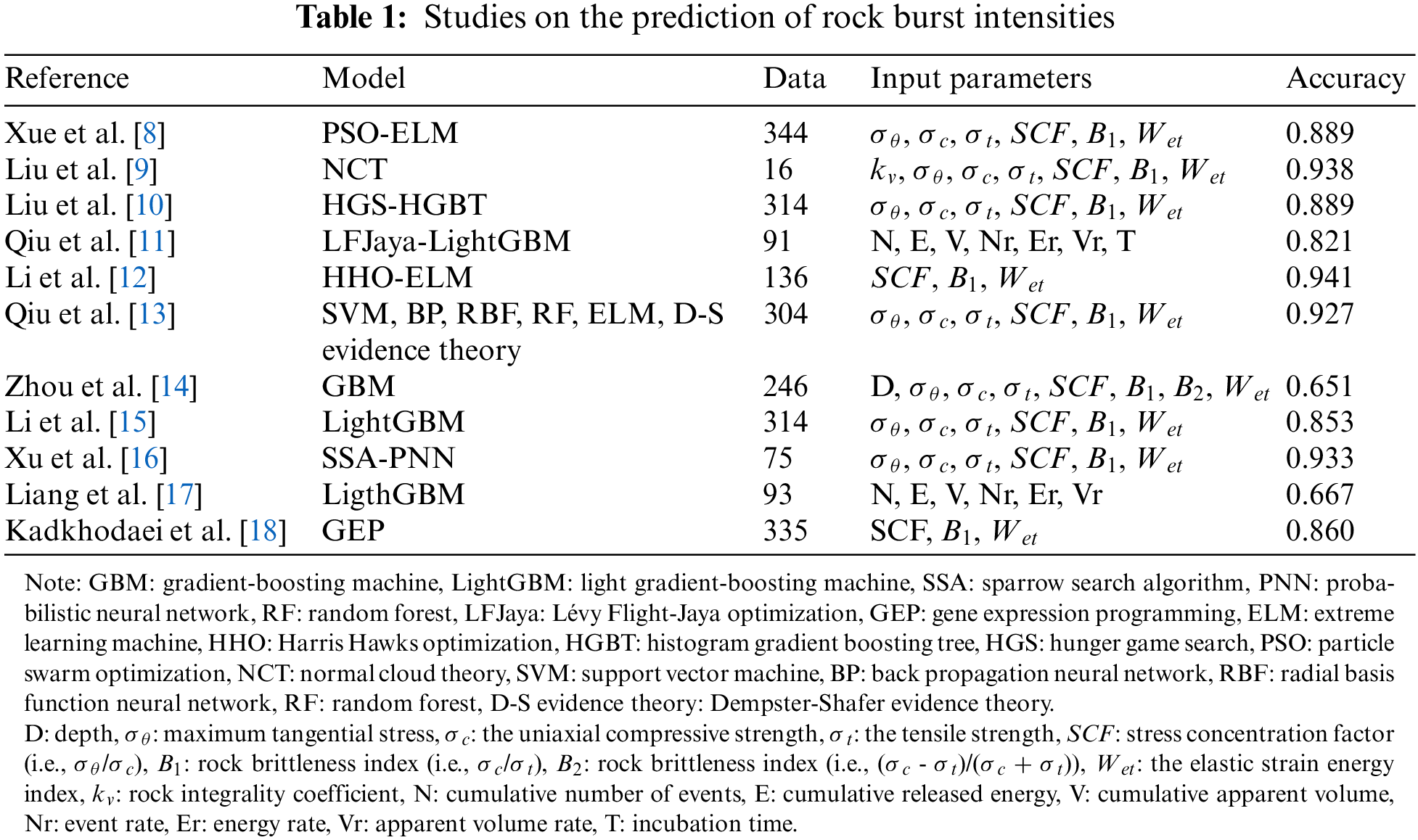
In summary, the above literature review provides a comprehensive overview of the development of machine learning-based approaches for rock burst prediction in underground engineering. Specifically, neural network-based and tree-based models are commonly employed in this field. The main limitation of these models is their subpar performance in predicting rock burst intensities. Most models have an accuracy below 0.90, and some even perform poorly, for example, [14] and [17]. Thus, to tackle this issue, this study seeks to develop a hybrid LightGBM model for achieving high-accuracy prediction of rock burst intensities. Furthermore, this study employs comprehensive model interpretation techniques to unveil the predominant factors influencing rock burst prediction when utilizing the established LightGBM model.

2  Materials

2.1 Data Source

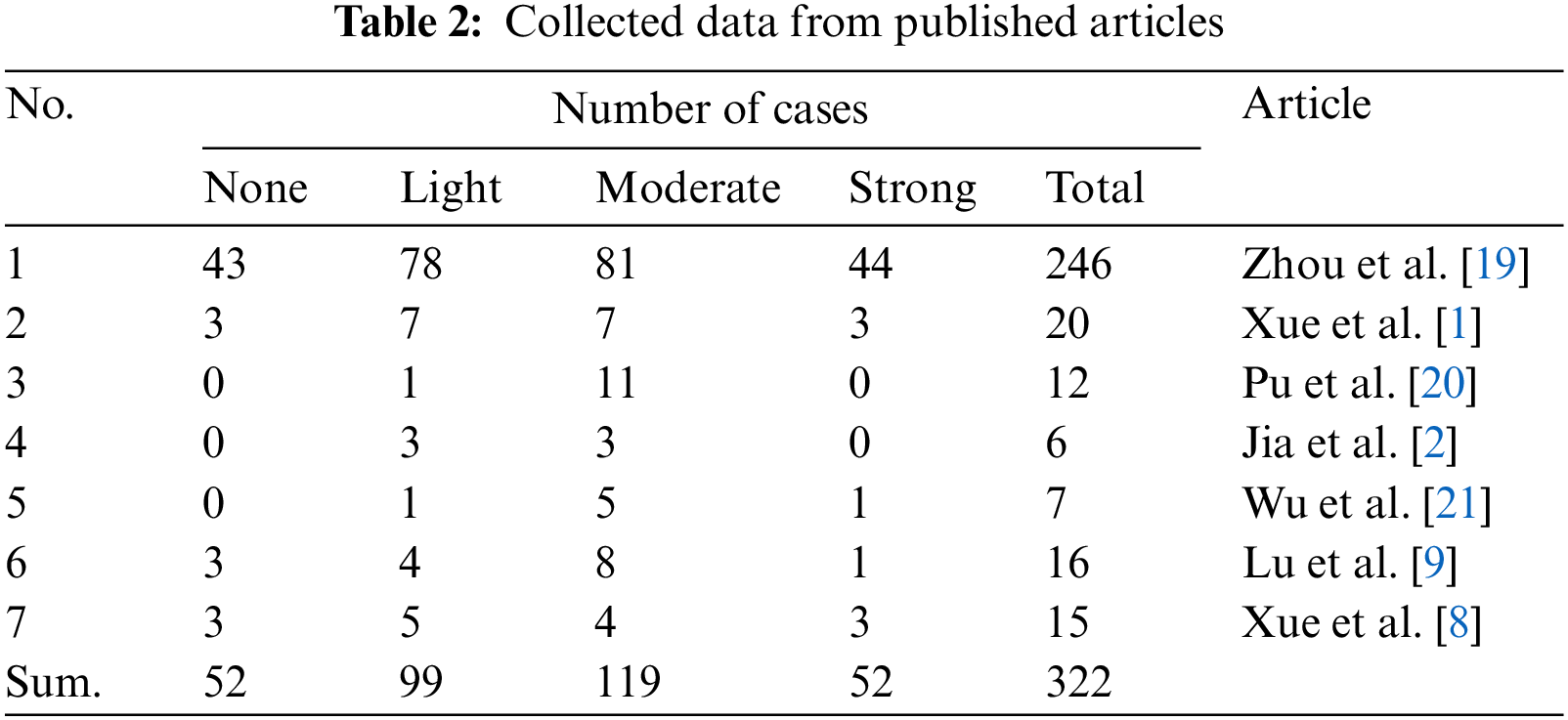
This study collected five sets of data collected from the published articles, which are 246 samples from [19], 20 samples from [1], 12 samples from [20], 6 samples from [2], 7 samples from [21], 16 samples from [9], and 15 samples from [8]. Consequently, the entire dataset comprises 322 samples of rock bursts, which is shown in Table 2. Overall, 52 samples are recording the ‘None’ intensity of rock bursts, 99 samples recording the ‘Light’ intensity of rock bursts, 119 samples recording the ‘Moderate’ intensity of rock bursts, and 52 samples recording the ‘Strong’ intensity of rock bursts. The intensity of the rock bursts can be defined as below [22]:

● None: the least severe level of rock bursts, which is characterized by the absence of any significant damage to the surrounding structures or personnel. The rock mass may experience some minor cracking or deformation, but there is no widespread damage.

● Light: the second least severe level of rock bursts, which is characterized by minor damage to the surrounding structures and personnel. The rock mass may experience some cracking or deformation, but there is no widespread damage.

● Moderate: the third level of rock burst intensity, which is characterized by moderate damage to the surrounding structures and personnel. The rock mass may experience significant cracking or deformation, and there may be some injuries to personnel.

● Strong: the fourth level of rock burst severity, which is characterized by extensive damage to the surrounding structures and personnel. The rock mass may experience large-scale cracking and deformation, and there may be multiple injuries or fatalities. Factors such as a very weak rock mass, an extremely high-stress condition, or a very low presence of discontinuities may cause the strong intensity of rock bursts.

The collected dataset comprises seven inputs and one output. The inputs include seven rock properties: maximum tangential stress (σθ), uniaxial compressive strength (σc), uniaxial tensile strength (σt), elastic strain energy index (Wet), stress concentration factor (SCF), rock brittleness index (B1), and rock brittleness index (B2). Here, according to the definitions in [22,23], SCF = σθ /σc, B1 = σc/σt and B2 = (σc – σt)/(σc + σt). SCF quantifies the increase in stress around discontinuities within a material; B1 measures the rock’s tendency to fracture under stress based on its uniaxial compressive and tensile strengths; B2 evaluates brittleness based on the ratio of the difference between uniaxial compressive strength and tensile strength to their sum.

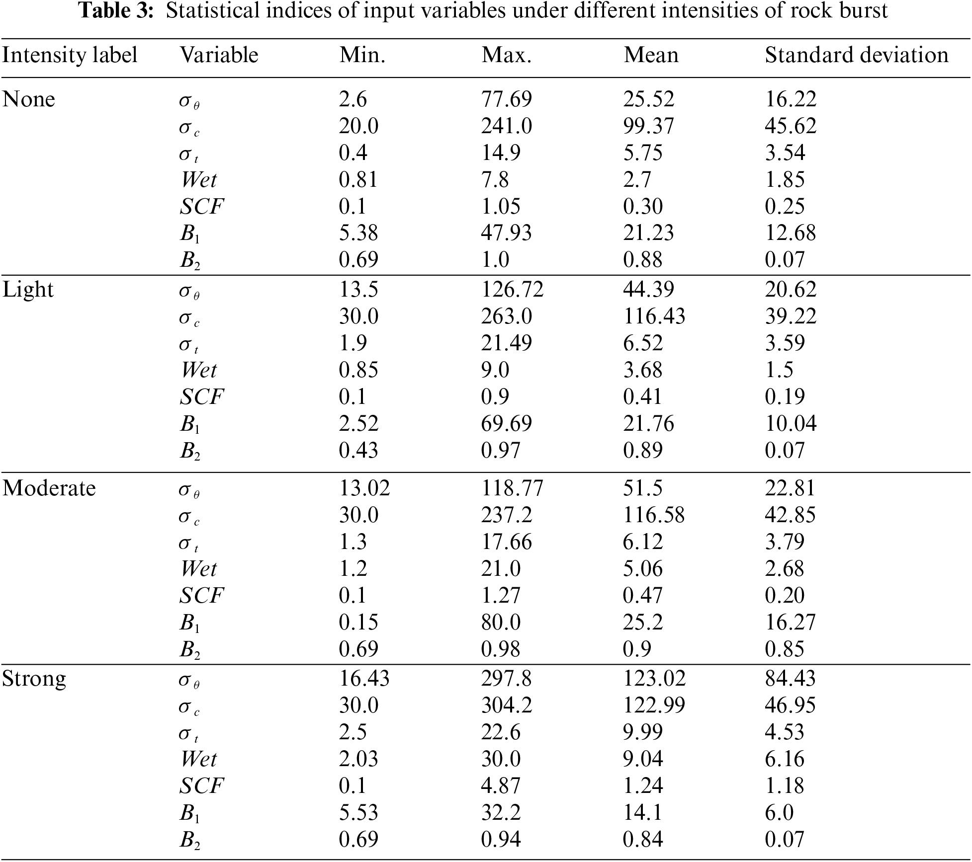
Typically, rock properties are deemed as the critical factors affecting the intensity of rock bursts in underground projects [19,22,24]. For example, rock properties determine the strength and deformability of the rock mass. Stronger and more deformable rocks are less likely to rock burst. Rock properties influence the stress distribution around the excavation. High stresses in the rock mass increase the risk of rock bursts. Rock properties affect how the rock mass fails. Some rock types are more prone to brittle failure, which is associated with rock bursts. Based on this, this study aims to identify the intensity of rock bursts via the rock properties and analyze their particular impacts on the rock burst. Table 3 summarizes statistical indices of these variables under four intensities of rock burst.

2.2 Data Pre-Processing

This study aims to build a machine learning-based classification model to predict the intensity of rock bursts. Before training the classification model, a critical step is to implement data cleaning on the raw dataset. Data cleaning is the process of identifying and correcting errors, inconsistencies, and inaccuracies in data. It can significantly improve the performance and accuracy of the classification model.

One powerful tool commonly employed in data cleaning is the boxplot, also known as a box-and-whisker plot. This graphical representation offers a clear and intuitive way to visualize the distribution of data points. A boxplot provides a summary of key statistical characteristics within a dataset, including the median, quartiles, and potential outliers [25,26]. This study applied the boxplot to input variables of the entire dataset, whatever the intensity of the rock burst. As a result, Fig. 1 illustrates the potential outliers in each variable. For variable σθ, values larger than 126 MPa are identified as outliers; for variable σc, values larger than 235 MPa are identified as outliers; for variable σt, values larger than 18.0 MPa are identified as outliers; for variable SCF, values larger than 1.26 are identified as outliers; for variable B1, values larger than 49.5 are identified as outliers; for variable B2, values smaller than 0.69 are identified as outliers; for variable Wet, values larger than 10.5 are identified as outliers. To ensure the accuracy and generalizability of the rock burst prediction model, data samples involving outliers are excluded from the raw dataset even though they can occur in operational contexts. This is because the machine learning-based prediction model is sensitive to extreme values (i.e., outliers) in the dataset. Outliers can significantly skew the model’s learning process, leading to overfitting where the model excessively learns from these anomalies instead of recognizing general patterns [27].

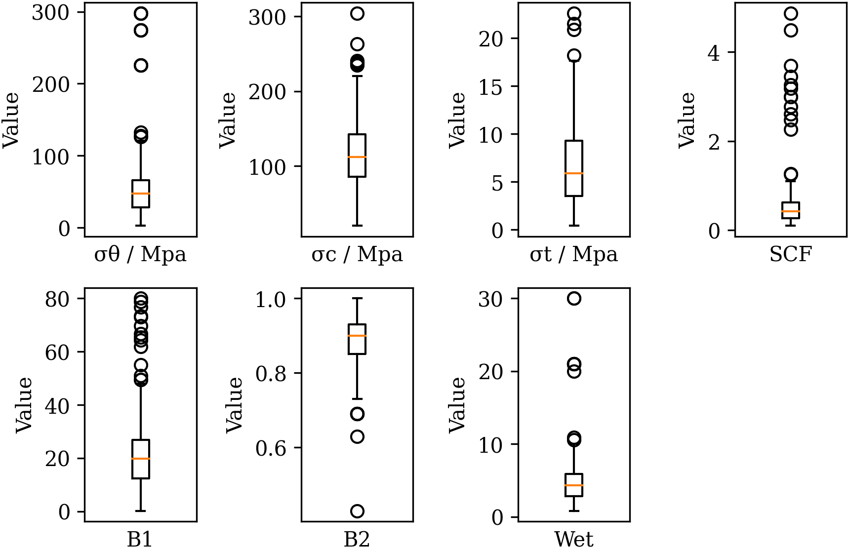
Figure 1: Boxplot of numerical variables

After removing all identified outliers from the raw dataset, we eventually obtained 268 data samples for studying rock bursts. Fig. 2 shows the histogram of the cleaned dataset under four intensities of the rock burst: None, Light, Moderate, and Strong. Intuitively, the cases of ‘Light’ and ‘Moderate’ rock bursts are in the vast majority, while the cases of ‘Strong’ rock burst are in the minority.

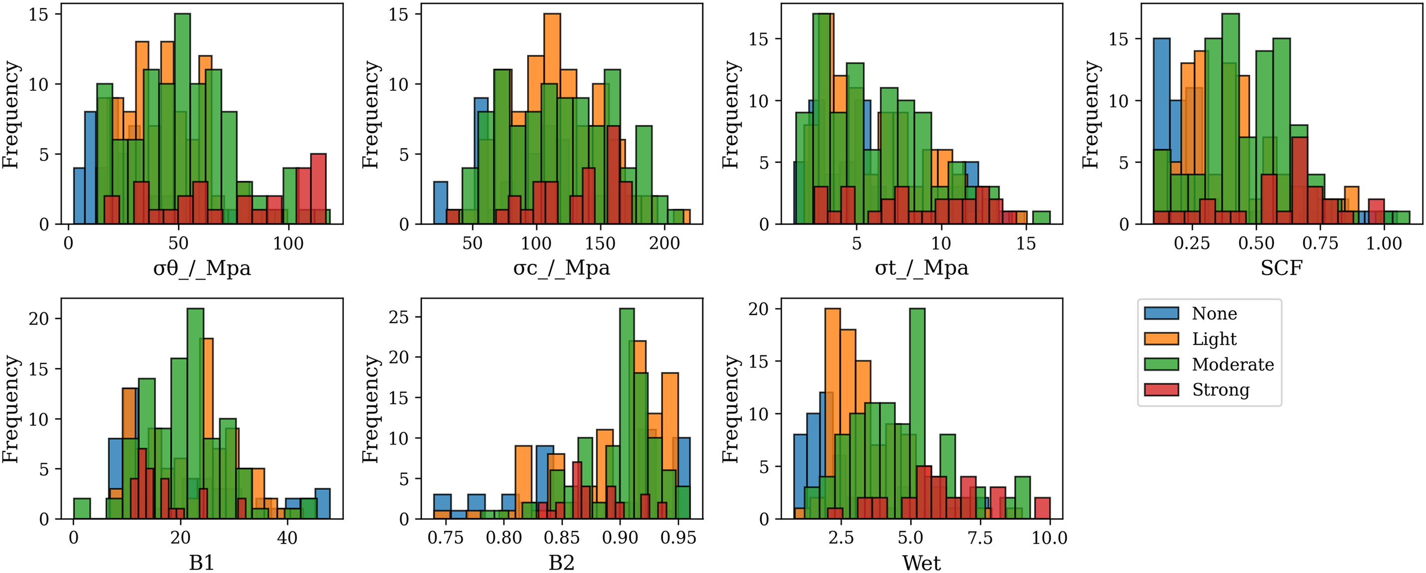
Figure 2: Histogram of numerical variables under four intensities of rock burst

Before conducting machine learning, splitting the data into training and testing sets is a critical step, which helps to prevent overfitting of the trained machine learning model. Hence, this study splits the dataset into two parts: 80% (214 samples) used for training the classification model, and 20% (54 samples) used for evaluating the model’s performance. The training set serves as the foundation upon which the classification model is constructed. The model uses the training data to understand patterns, relationships, and underlying structures within the information. On the other hand, the testing set plays a pivotal role in assessing the model’s performance and generalization capabilities. It serves as a benchmark, allowing us to evaluate how well the model can make predictions on new, unseen data.

To visualize the distribution of the training and testing sets, Principal Component Analysis (PCA) is employed herein. PCA is a powerful statistical technique used in dimensionality reduction [28,29]. It helps uncover the underlying structure in a dataset by transforming the original variables into a new set of variables, called principal components. These principal components are linear combinations of the original variables and are chosen in such a way that they capture the maximum variance in the data. Fig. 3 displays the distributions of the training and testing sets under four intensities of rock burst. Overall, the distribution between the training and testing sets is roughly similar. The training set has a higher distribution of two principal components than the testing set, which indicates the training set can embrace the scope of the testing set. This may anticipate that the classification model trained on the training set would have a promising generalization ability on the testing set.

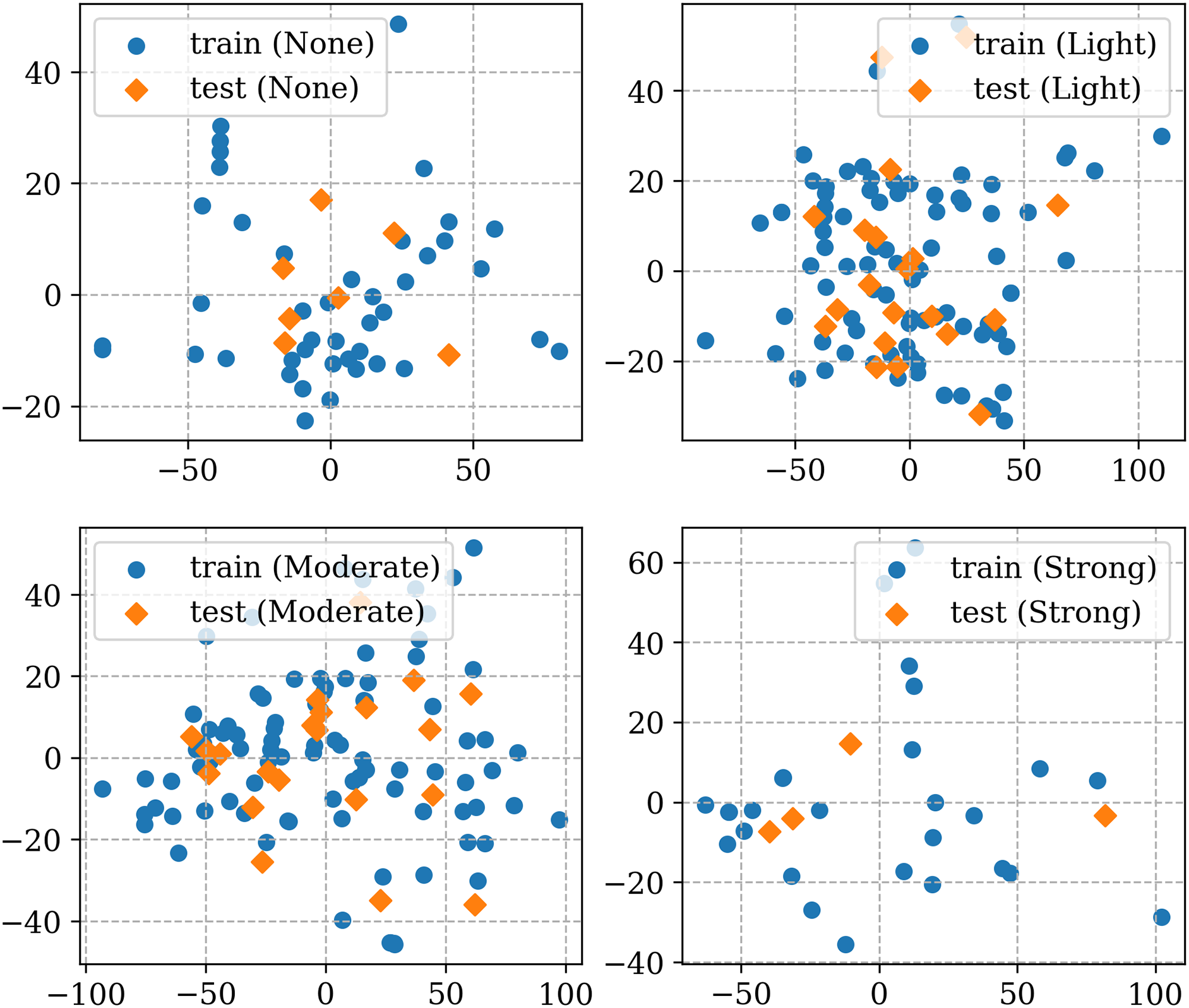
Figure 3: Comparison of data distributions between the training and testing sets via PCA

3  Methods

3.1 LightGBM

LightGBM (Light Gradient Boosting Machine) is a powerful and efficient gradient-boosting framework that has gained widespread popularity in machine learning and data science [30]. It was developed by Microsoft and is an open-source project. LightGBM is designed to address some of the limitations of traditional gradient boosting methods and is particularly well-suited for large-scale, high-dimensional datasets. LightGBM builds on the fundamental concepts of gradient boosting, which is an ensemble learning technique. The cores of the LightGBM model include [31]:

● Decision trees: LightGBM uses decision trees as the base learners. These trees are constructed sequentially to improve predictive accuracy.

● Gradient Boosting: Gradient boosting involves optimizing a loss function by adding decision trees in a way that minimizes the error. LightGBM uses gradient-based optimization techniques for this purpose.

● Leaf-Wise Growth: LightGBM employs a leaf-wise tree growth strategy, which differs from traditional level-wise growth. This approach often leads to faster convergence and better results.

● Histogram-Based Learning: LightGBM employs histogram-based techniques to speed up the training process. It discretizes continuous features into bins, which reduces memory usage and improves training speed.

● Exclusive Feature Bundling: LightGBM uses a technique called exclusive feature bundling to reduce the dimensionality of the data. This can lead to faster training and better performance on sparse datasets.

The LightGBM model has several remarkable advantages. For example, it has fast computational speed and efficiency, making it suitable for large datasets and real-time applications. LightGBM can achieve competitive or superior predictive accuracy compared with other tree-based machine learning algorithms. It also supports parallel and distributed computing, further enhancing its scalability. LightGBM achieves algorithmic control via several primary hyperparameters shown below [32]:

● n_estimators: the number of boosting iterations or trees to build in the LightGBM model. It controls the overall complexity and capacity of the model.

● learning_rate: the step size at which the gradient boosting algorithm adapts during training. It scales the contribution of each tree to the final prediction.

● max_depth: the maximum depth or level that an individual tree can reach during training. It controls the complexity of each tree.

● num_leaves: the maximum number of leaves (terminal nodes) in each tree. It controls the granularity of the tree structure.

● colsample_bytree: the fraction of features (columns) to be randomly selected for building each tree. It can be effective in reducing overfitting and improving generalization.

● min_child_samples: the minimum number of data points required in a leaf node. It can control the depth of the trees and help prevent them from becoming too deep, which can lead to overfitting.

These hyperparameters play critical roles in controlling the behavior of the LightGBM model. Tuning them correctly is essential for achieving good model performance, and the optimal values can vary depending on the specific dataset and problem.

3.2 Optimization Algorithm

3.2.1 Coati Optimization Algorithm

The Coati Optimization Algorithm (COA), proposed in 2023, is a new bio-inspired metaheuristic algorithm that is inspired by the natural behaviors of coatis [33]. COA mimics two natural behaviors of coatis, which are the strategies of hunting iguanas and escaping from predators. The mathematical model of COA is introduced as follows:

1) Initialization process

In the COA framework, each coati constitutes a candidate solution to the problem under consideration. The COA’s initialization phase entails a random positioning of the coatis within the search space, a process elucidated by Eq. (1).

xi,j=lj+r⋅(uj−lj),i=1,2,…,N,j=1,2,…,M(1)

where xi,j represents the candidate member/solution, lj is the lower bound, uj is the upper bound, r is a random value between 0 and 1, M is the dimension of the target problem.

2) Exploration phase: strategy of hunting iguanas

The exploration phase is to update the coati population within the search space, predicated upon the emulation of their foraging strategy employed when pursuing iguanas. Within the framework of COA, the algorithm stipulates that the optimal position within the population corresponds to the position of the iguana. Furthermore, it is postulated that an equitable division of coatis entails half of the population rising from the tree, while the remaining half remains positioned on the ground, anticipating the iguana’s eventual descent.

Eq. (2) simulates the mathematical process of the coatis rising from the tree:

XiP1:xi,jP1=xi,j+r⋅(Iguanaj−I⋅xi,j),for  i=1,2,…,N2,andj=1,2,…,M(2)

where XiP1 denotes the new position of the ith coati, xi,jP1 denotes the jth dimension of the XiP1, Iguanaj represents the position of the iguana in the search space, I is an integer that is randomly selected from {1, 2}, ⌊⋅⌋ represents the greatest integer function.

When the iguana falls down a random place on the ground, the coatis instantly move in the search space (i.e., the ground). This mathematical process is characterized by Eqs. (3) and (4).

IguanaG:IguanajG=lj+r⋅(uj+lj),j=1,2,..,M(3)

XiP1:xi,jP1={xi,j+r⋅(IguanajG−I⋅xi,j),FIguanaG<Fi,xi,j+r⋅(xi,j−IguanajG),else,for  i=⌊N2⌋+1,⌊N2⌋+2,…,Nandj=1,2,…,M(4)

where IguanaG denotes the iguana on the ground, IguanajG is the jth dimension of the IguanaG, FIguanaG denotes the objective function value of the IguanaG, Fi denotes the objective function value of the xi,jP1.

3) Exploitation phase: strategy of escaping from predators

The exploitation phase is to update the natural behavior of the coatis when encountering their predators and escaping from them. When a coati encounters the predator, it will move to a safe position that is close to its current position. Eqs. (5) and (6) simulate such a mathematical process.

ljlocal=ljt,ujlocal=ujt, where t=1,2,..,T(5)

XiP2:xi,jP2=xi,j+(1−2r)⋅(ljlocal+r⋅(ujlocal−ljlocal)),i=1,2,…,N,  j=1,2,…,M(6)

where XiP2 is the new position of the ith coati in the exploitation phase, xi,jP2 represents the jth dimension of the XiP2, ljlocal and ujlocal are the local lower bound and local upper bound, respectively, t is the current iteration.

3.2.2 Pelican Optimization Algorithm

The Pelican Optimization Algorithm (POA), proposed in 2023, is a population-based metaheuristic optimization algorithm inspired by the hunting behavior of pelicans [34]. The algorithm works by simulating the steps of pelicans hunting for fish: 1) pelicans fly in a flock and search for fish; 2) when a pelican spots a fish, it dives down to catch it; 3) if the pelican is successful, it returns to the flock with the fish; 4) if the pelican is unsuccessful, it returns to flock empty-handed. The mathematical steps of the algorithm are as follows:

1) Initialize a population of solutions randomly

In the POA, each population member represents a potential candidate solution. Initially, population members are randomly created in the solution domain according to the lower and upper bounds of a particular problem.

xi,j=lj+rand⋅(uj−lj),i=1,2,…,N,  j=1,2,…,M(7)

where xi,j represents the candidate member/solution, lj is the lower bound, uj is the upper bound, rand denotes a random value between 0 and 1, N is the number of candidate members, M is the dimension of the target problem. After initializing the pelican population, POA began to mimic the hunting behaviors of pelicans: moving towards prey and winging on the water surface.

2) Exploration phase: moving towards prey

During the initial phase of the POA, pelicans scout for prey by surveying the search space and subsequently advancing toward it. Notably, the prey’s position within the search space is randomly generated, further augmenting the algorithm's exploration potential. Eq. (8) is used to characterize the abovementioned pelican’s strategy in moving the place of prey, as well as updating the positions of the pelicans in the search space.

xi,jP1={xi,j+rand⋅(pj−I⋅xi,j),Fp<Fixi,j+rand⋅(xi,j−pj),else(8)

where xi,jP1 represents the candidate member in the first phase (exploration phase), I is a value that randomly equals 1 or 2 as the iteration of POA, pj is the location of the prey, and Fp is the objective function value of the prey. Regarding the parameter I, it enables more displacement for a pelican member when it is equal to 2, which enhances the exploration ability of the POA.

3) Exploitation phase: winging on the water surface

During the POA’s second phase, pelicans unfurl their wings atop the water’s surface as they begin amassing their captured prey in their specialized throat pouch. Notably, pelicans extend their wings on the water’s surface solely when they are close to their prey. This ensures that the pelicans are only able to catch the fish that are in the immediate vicinity, which increases the efficiency of the algorithm.

The aforementioned strategy of the pelican strategy in catching prey is mathematically simulated in Eq. (9), which is used to model the movement of the pelicans’ wings and the fish and to update the positions of the pelicans in the search space.

xi,jP2=xi.j+R⋅(1−tT)⋅(2⋅rand−1)⋅xi,j(9)

where xi,jP2 represents the candidate member in the first phase (exploitation phase), R is a constant that equals 0.2, t is the current iteration, and T is the maximum iteration. Here, R⋅(1−tT) represents the radius that the candidate member locally searches. It benefits to enhance the exploitation ability of the POA.

Once all population members have been revised according to the outcomes of the first and second phases, the algorithm identifies the best candidate solution for the objective function values. Subsequently, the algorithm advances to the next iteration, where it reiterates the procedures outlined in Eq. (8) through Eq. (9). This iterative process persists until the predefined stopping criterion is satisfied.

3.3 Research Step

This study aims to optimize the hyperparameters of the LightGBM model via two metaheuristic-based optimization algorithms—COA and POA. Fig. 4 presents the methodology of this study, which includes two parts: the preliminary phase and the training phase.

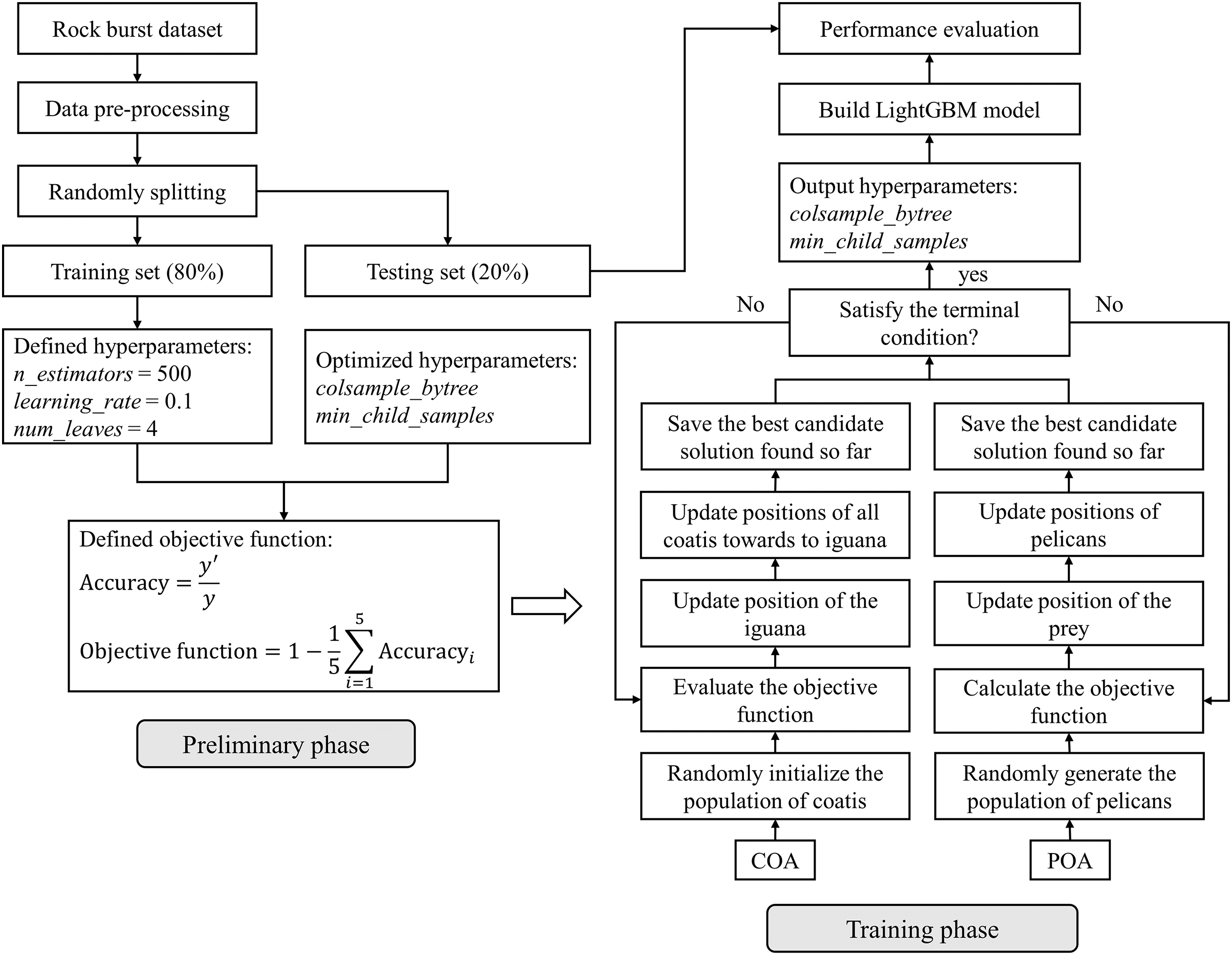
Figure 4: Flowchart of the methodology of this study

The preliminary phase includes:

● Data preparation: This process commences with rigorous data curation, involving outlier identification and removal, ensuring the robustness of the dataset. The data are then randomly divided into training (80%) and testing sets (20%), a split designed to balance between model training and testing, as detailed in Section 2.

● Setting hyperparameters of the LightGBM model: Key hyperparameters such as n_estimators, learning_rate, max_depth, and num_leaves are set to predefined values (500, 0.1, 4, and 3, respectively) based on preliminary tests that indicate optimal model performance at these levels. For hyperparameters such as colsample_bytree and min_child_samples, adjustable within the ranges of (0.2, 0.8) and (1, 20), respectively, their optimization is based on the COA and POA algorithms.

● Defining optimization algorithms (COA and POA): COA and POA are selected for their efficiency and user-friendly attributes. In this study, they are configured with just two parameters—population size and the number of iterations—to streamline the optimization process while maintaining algorithm effectiveness.

● Determining the objective function: The objective function, crucial for guiding the optimization algorithms, is delineated in Eqs. (10) and (11). It encapsulates the minimization problem central to this study. Five-fold cross-validation on the training set is integrated into the model training process to underpin the LightGBM model's generalizability. The test set remains unseen by the LightGBM throughout the entire process. The term ‘Accuracy’ denotes the predictive accuracy of the LightGBM model; y′ denotes the number of correct predictions; y denotes the number of the entire predictions.

Accuracy=y′y(10)

Objective function=1−15∑i=15Accuracyi(11)

The training phase includes:

● Initializing optimization algorithms: The COA and POA are initialized with different population sizes (20, 40, and 60) to explore the impact of this parameter on optimization efficacy. The number of iterations for both algorithms is uniformly set to 100, balancing thorough exploration with computational efficiency.

● Training the model: The model training involves iterative calculations and updates of the objective function, alongside refining local and global optimal solutions. This dynamic approach allowed for continuous improvement in the hyperparameter values throughout the optimization process.

● Check-stopping criterion: The optimization is configured to terminate upon reaching the maximum iteration count of 100. This criterion was chosen to ensure a thorough search of the hyperparameter space without excessive computational demand.

● Extracting results: The best values for colsample_bytree and min_child_samples are extracted. Additionally, objective function values, running times, and diversity metrics of the algorithms are recorded, providing a comprehensive overview of the optimization process’ effectiveness and efficiency.

All the aforementioned models or algorithms are designed and implemented based on Python programming.

4  Results and Discussion

This section aims to evaluate and select the best predictive model for estimating the intensity of the rock burst. First, the modeling process is discussed in detail, including the training and evolution of the algorithms: COA and POA. Then, the optimal hyperparameters of the LightGBM are determined. Lastly, the predominant factors affecting the intensity of the rock burst are identified.

4.1 Analysis of the Optimization Process

As mentioned previously, two optimization algorithms (COA and POA) are used to determine the optimal hyperparameters of the LightGBM model. For each algorithm, this study sets its population size as 20, 40, and 60, aiming at encouraging more exploration of the search space by maintaining diverse solutions. Fig. 5 shows the running time of two optimization algorithms with different population sizes. ‘POA-20’ spends the minimal running time, followed by ‘COA-20’. ‘COA-60’ spends the maximal running time due to its large population size. Overall, a consensus is that the larger the population size, the more time-consuming the calculation will be.

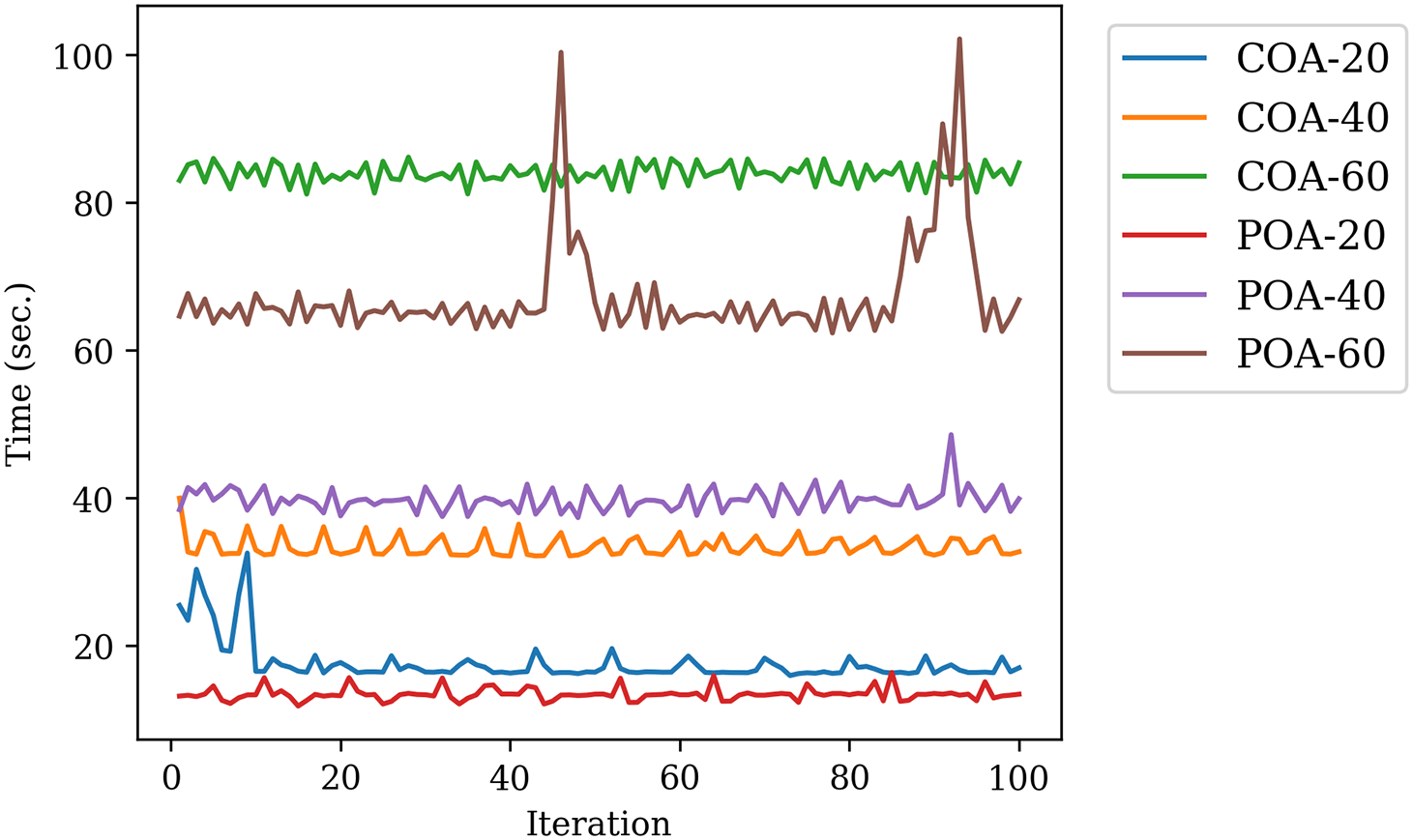
Figure 5: Running time of the model training

Fig. 6 shows the population diversity of two optimization algorithms with different population sizes. Intuitively, as the optimization algorithm progresses through iterations, there is a noticeable reduction in the diversity of the population. This decrease in diversity is often a sign that the algorithm is converging toward a specific region of the solution space [35]. Overall, the populations of all trials are becoming homogeneous and concentrating on a particular solution during the entire iteration. We also find that COA has a higher diversity than POA for each population size when the iteration is after 60.

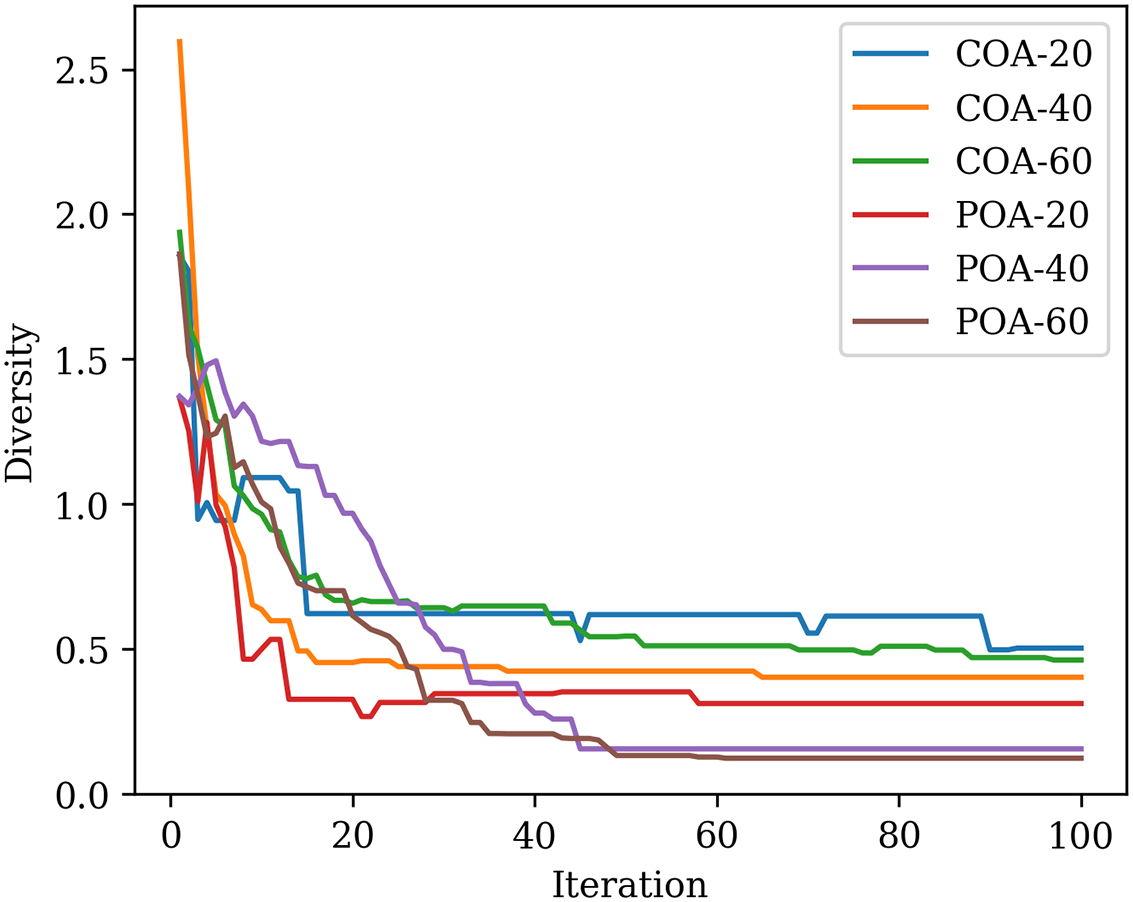
Figure 6: Evolution of the population diversity

Fig. 7 shows the exploitation and exploration rates of two optimization algorithms with different population sizes. The exploitation rate represents the emphasis placed on refining and intensifying the current solutions within the search space. High exploitation rates tend to lead the algorithm towards local optima. The exploration rate indicates the degree to which the algorithm is willing to explore new and unexplored regions of the search space. A high exploration rate implies that the algorithm is more exploratory, actively searching diverse areas of the solution space [36]. Overall, all trials show outstanding results in the evolution of the exploitation and exploration rates. This proves that the COA and POA have excellent abilities to accomplish local and global searching.

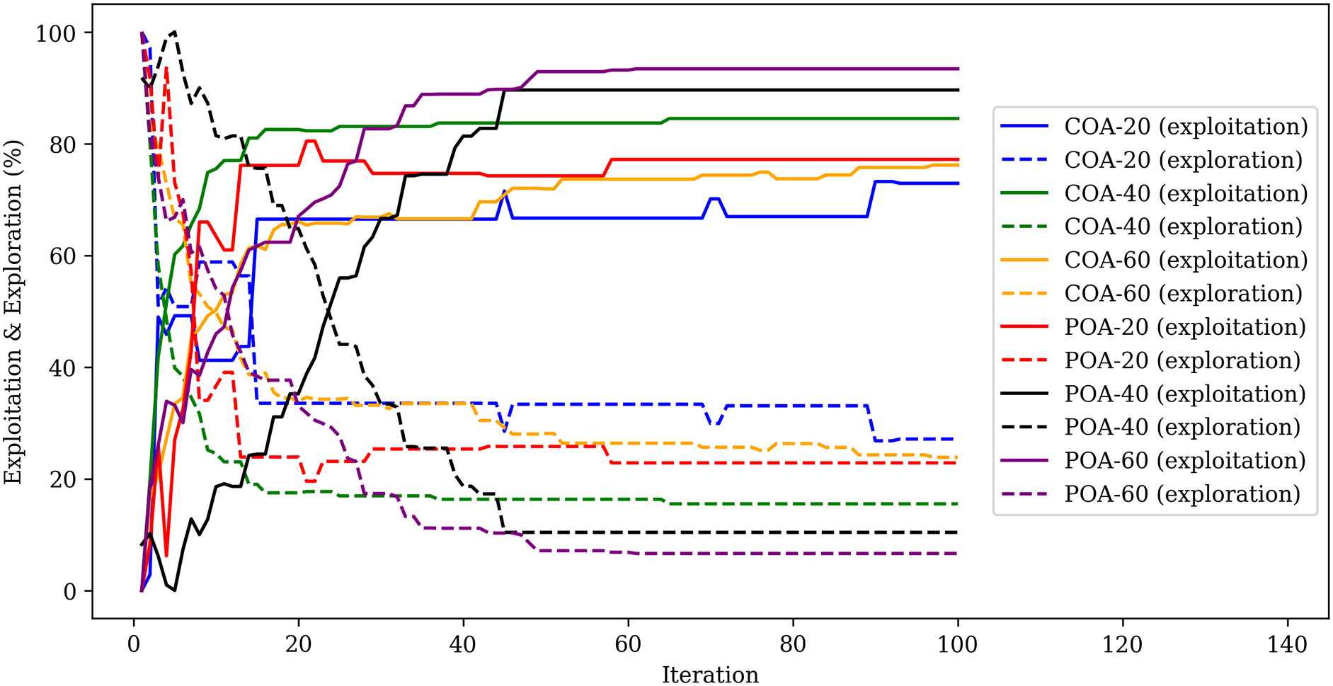
Figure 7: Evolution of the exploitation and exploration rates

Fig. 8 shows the iteration process of these two algorithms. We find that all models converged to final values until the 40th iteration. The iterations of all trials exhibit the trend of a steep slope, indicating that they fast converged to the final solution. Table 4 shows the obtained hyperparameters of the LightGBM model optimized by various algorithms. Since ‘COA-60’ has the minimal objective function value, it is thereby regarded as the optimal hyperparameter for the LightGBM model. The LightGBM model will be built based on these two optimal hyperparameters. Fig. 9 presents the position of each solution in the search space. We find that the hyperparameter min_child_samples shows a more significant role in controlling the performance of the LightGBM model. This is because the performance of the LightGBM has no apparent changes when the min_child_samples is equal to 17, even though the colsample_bytree changes between 0.2 and 0.35.

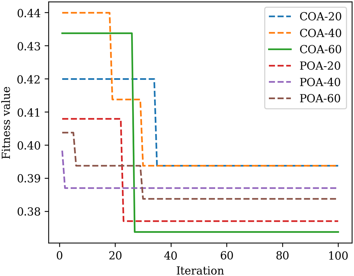
Figure 8: Iteration process of two optimization algorithms

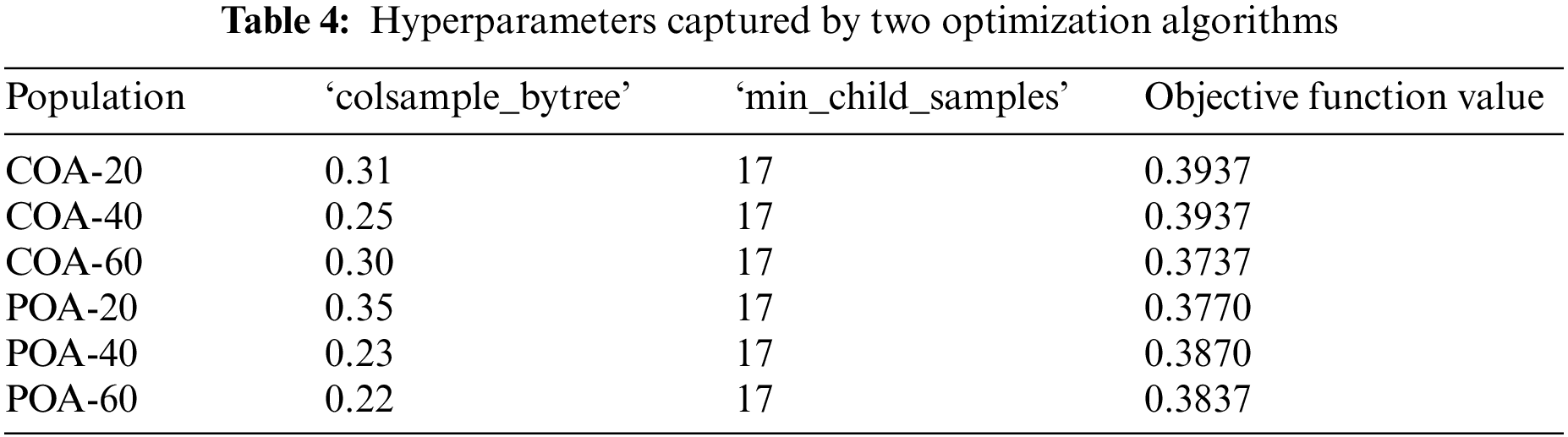
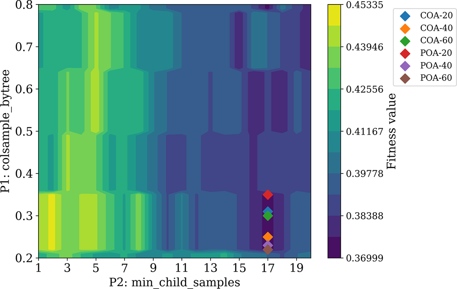
Figure 9: Solutions in the search space

4.2 Model Performance Evaluation

After obtaining the optimal hyperparameters of the LightGBM model, a crucial work is to examine its accuracy and performance. This study utilizes several common metrics to evaluate the model’s performance, which are accuracy, precision, recall, and F1 score [37]. The mathematical models of these metrics are shown as follows:

Accuracy=y′y(12)

Precision=TPTP+FP(13)

Recall=TPTP+FN(14)

F1=2×Precision×RecallPrecision+Recall(15)

where true positives (TP) represent instances where the model correctly identifies a positive outcome, false positives (FP) occur when the model incorrectly identifies a positive outcome that is not present, true negatives (TN) represent instances where the model correctly identifies a negative outcome, and false negatives (FN) occur when the system fails to detect a true positive outcome. These four metrics play pivotal roles in evaluating the precision, recall, F1 score, and overall accuracy of classification models.

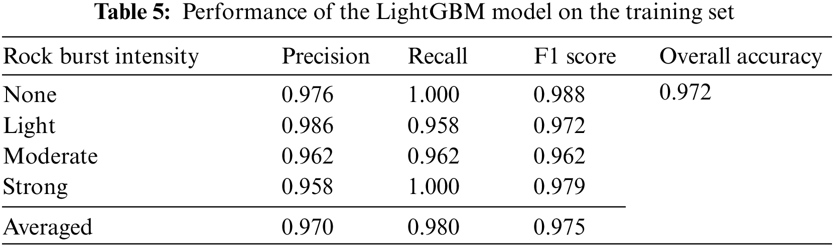
Tables 5 and 6 list the predictive performance of the LightGBM model on the training and testing sets, respectively. We find that the LightGBM model has an overall accuracy of 0.972 and 0.944 on the training and testing sets, respectively. Its performance on each subclass—the independent intensity of rock burst—is also promising. Additionally, we also find that the LightGBM model can exhaustively correctly predict the ‘None’ and ‘Strong’ intensities of rock burst on the testing set. This proves that the built LightGBM model with good predictive ability consistently achieves a high level of accuracy when tested on new, unseen data.

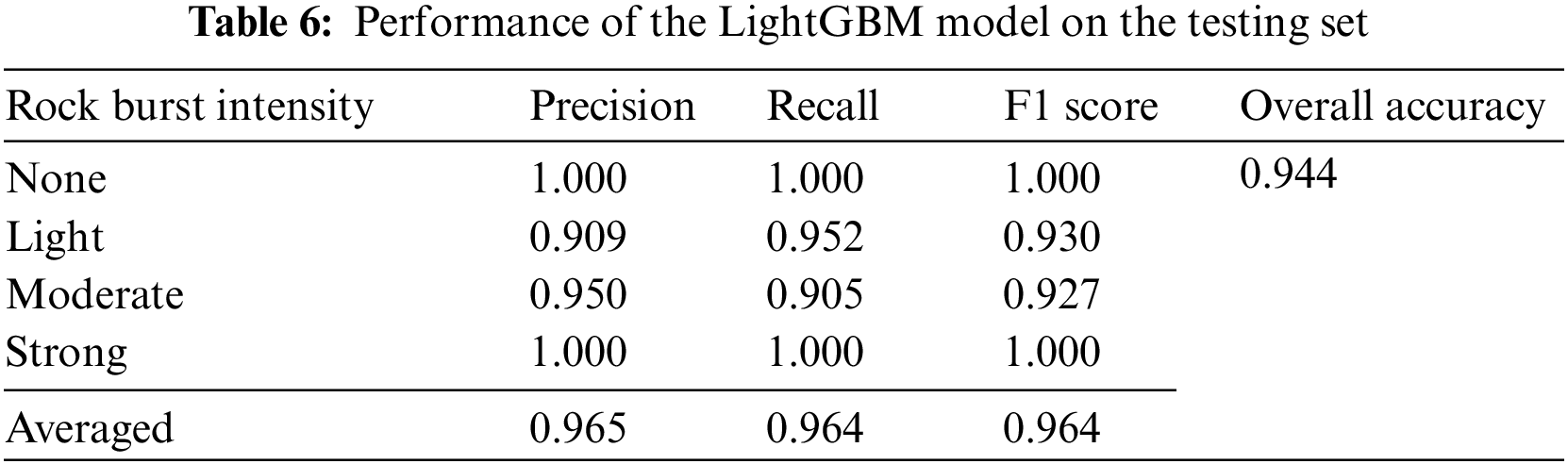
To further assess the effectiveness of the LightGBM model, this study compared it with previously published works. For example, Liang et al. used 93 microseismic data, which are related to short-term rock bursts, to train a LightGBM model [17]. However, the prediction accuracy of their LightGBM model is unsatisfactory, with an accuracy of only 0.667. Qiu et al. also used 91 microseismic data to develop a hybrid LightGBM model that combined with the Lévy Flight-Jaya optimization algorithm [11]. The prediction accuracy of their hybrid LightGBM model is 0.821. Another study, conducted by Li et al. [15], used the rock properties data to train a LightGBM model to predict rock bursts, resulting in an accuracy of 0.853.

Overall, the developed LightGBM models in previous works did not achieve a high accuracy in rock burst prediction. In contrast, our study introduces a more accurate LightGBM model, achieving training and testing accuracies of 0.972 and 0.944, respectively. Therefore, we conclude that our model demonstrates superior performance and reliability in predicting rock bursts when compared to existing models.

4.3 Model Verification

In this section, 12 sets of in-situ rock burst data, collected from two gold mines in China [38], are used to verify the generalization ability of the developed LightGBM model. These data were obtained from rock mechanics tests and field investigations. Among them, 7 sets of data were taken from Xincheng Gold Mine and 5 sets of data were taken from Sanshadao Gold Mine. Table 7 presents the rock properties and corresponding rock burst intensities. Seven variables, which are σθ, σc, σt, Wet, SCF, B1, and B2, are deemed as inputs of the LightGBM model, so the predicted rock burst intensities can be obtained accordingly. Fig. 10 illustrates the actual and predicted intensities of the rock burst. Intuitively, the LightGBM model can successfully predict most rock burst intensities, which demonstrates its good generalization ability on unseen data. It yields a prediction accuracy of 0.857 on Xincheng Gold Mine and 1.000 on Sanshadao Gold Mine, while its overall accuracy is 0.917. Consequently, this finding implies that the developed LightGBM model would have a promising perspective in the application in practical scenarios.

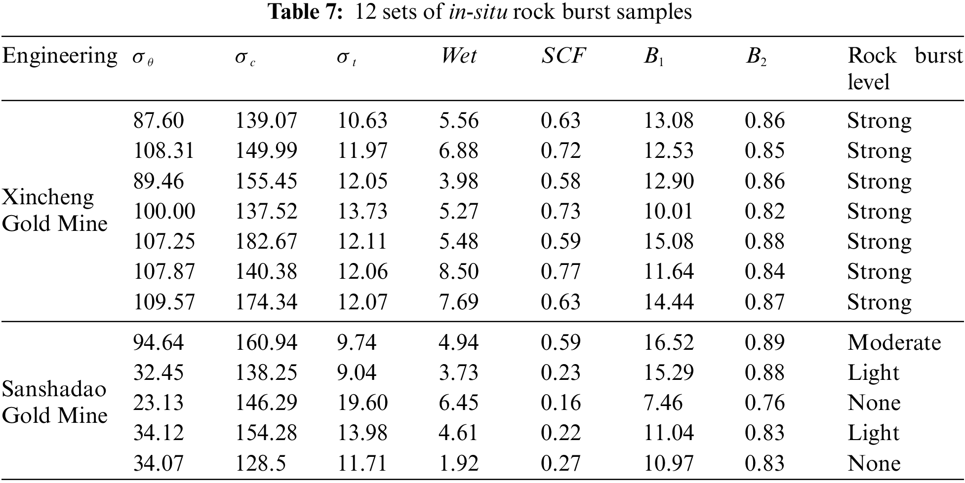
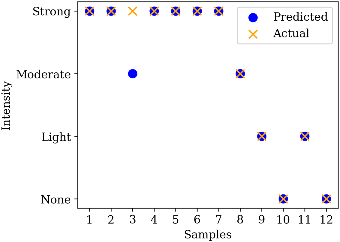
Figure 10: Actual and predicted intensities of rock burst

4.4 Model Interpretation

After successfully building the high-accuracy LightGBM model, it is crucial to interpret the model to understand the predominant factors that influence the occurrence of the rock burst. Considering the property of the LightGBM model, the importance of an individual feature can be extracted by counting the number of times that a feature is used in a model. In a nutshell, the more frequently the feature is used to split trees, the greater its significance is demonstrated [30]. Fig. 11 presents the importance of each feature/factor in predicting the intensity of the rock burst. Three predominant factors, namely uniaxial compressive strength (σc), stress concentration factor (SCF), and elastic strain energy index (Wet), have importance coefficients of 0.209, 0.192, and 0.176, respectively. The result of this study is consistent with some published articles. For example, Zhou et al. developed a random forest (RF) model to address the classification problem of the rock burst. The results indicate that Wet and SCF are the most sensitive factors affecting the occurrence of rock bursts [14]. Qiu et al. designed a hybrid extreme gradient boosting (XGBoost) model to predict short-term rock burst damage. They identify that SCF is one of the most significant factors contributing to rock burst prediction [39]. Wu et al. proposed a least squares support vector machine model to predict the probability of rock bursts. They used the Sobol index to implement factor sensitivity analysis and found that Wet is one of the most sensitive factors for predicting rock burst levels [21].

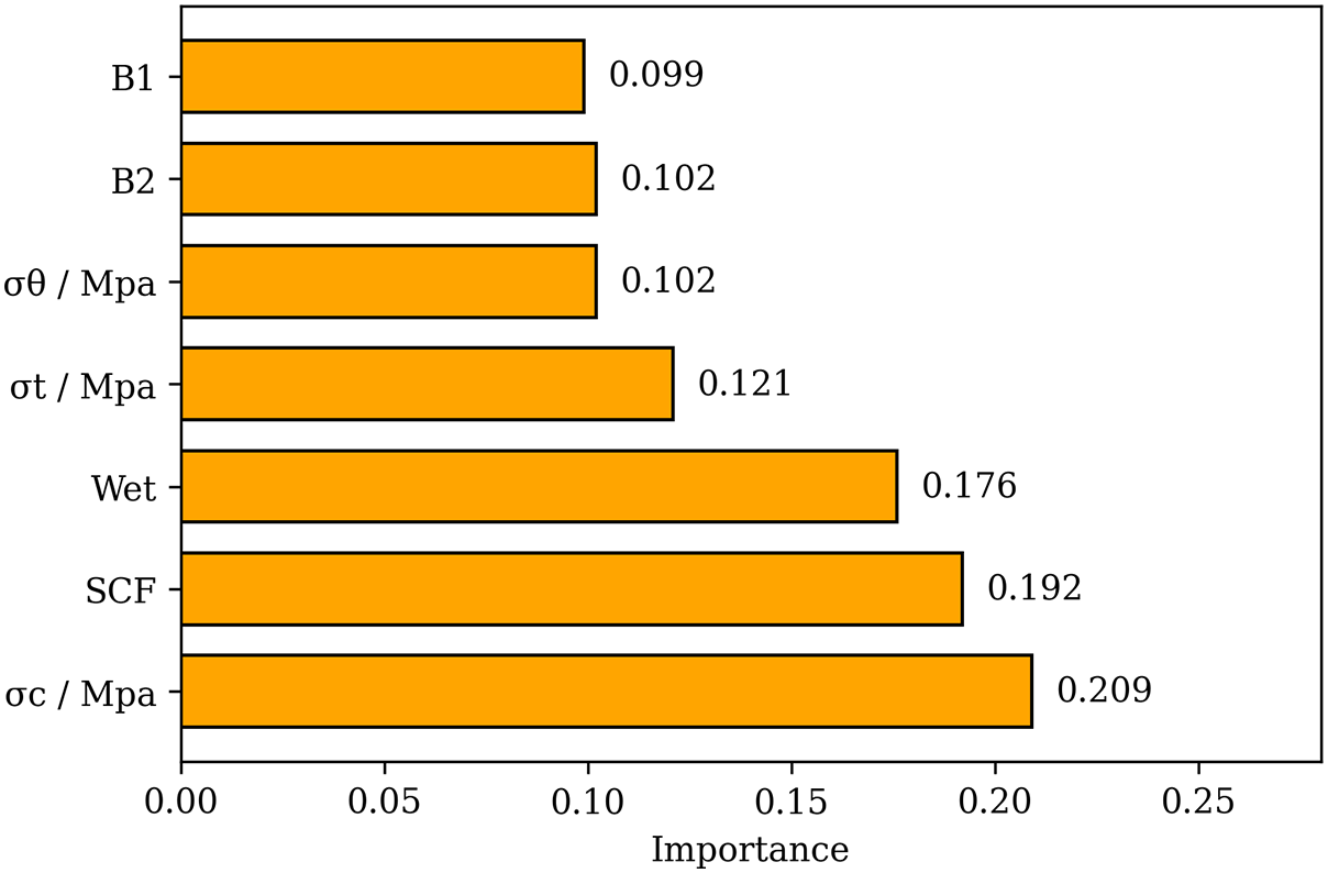
Figure 11: Feature importance in predicting the intensity of rock burst

Considering the significance of the aforementioned factors, our subsequent objective is to ascertain the distinct impact of these three factors in predicting the intensity of rock bursts. A partial dependence plot (PDP) is used to accomplish this objective. PDP is a powerful tool in the field of machine learning and predictive modeling, playing a crucial role in understanding and interpreting complex predictive models. It provides a comprehensive visual representation of how a specific feature or factor influences the predictions while keeping all other variables constant. Essentially, it allows one to grasp the isolated impact of one or more features on the model’s output, helping uncover relationships, patterns, and dependencies that might not be immediately apparent [40,41]. The steps for drawing PDPs are outlined below:

1.    Initially, the training set is prepared, and the established LightGBM model is fit on it.

2.    Factors such as σc, SCF, and Wet are selected to generate PDPs because they were previously identified as predominant factors affecting the rock burst prediction.

3.    For each selected factor, we systematically varied its value across its range while keeping all other factors constant. The LightGBM model then predicts the outcome of rock burst intensities for each of these modified instances, which forms the basis for the PDPs.

4.    The changes in the predicted outcome as a function of the varied factors are plotted, resulting in the PDPs. These plots visually represent how the predicted outcome is affected by changes in the factor’s values, while other factors are averaged out.

Fig. 12 illustrates the impact of uniaxial compressive strength (σc) in predicting the intensity of the rock burst. The vertical axis represents the probability of a rock burst occurring at a certain intensity. In a nutshell, the intensity with the highest probability will ultimately determine the predicted class—None, Light, Moderate, or Strong. Based on this, we find that the factor σc has a significant impact on ‘None’ and ‘Light’ intensities of rock bursts, because of the high probabilities of these two classes. When the value of σc is greater than 20 MPa but less than 96 MPa, the rock is at light risk of rock. When the value of σc is greater than 96 MPa but less than 220 MPa, the rock is at no risk of rock bursts—for the majority of cases. Additionally, we also find that there is no risk of occurring moderate and strong intensities of rock bursts as the σc increases from 20 to 220 MPa.

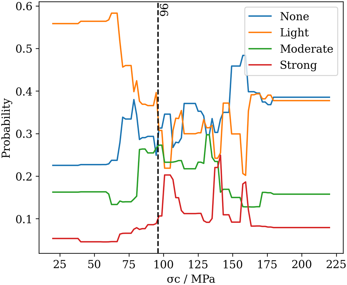
Figure 12: Impact of σc in predicting the intensity of rock bursts

Overall, there is a strong correlation between σc and rock burst potential. Rocks with lower uniaxial compressive strength are more likely to experience rock bursts. This is because a lower σc can make the rock more susceptible to fracturing and ultimately increase the risk of a rock burst happening.

Fig. 13 illustrates the impact of the stress concentration factor (SCF) in predicting the intensity of the rock bursts. The factor SCF has a significant impact on ‘None’, ‘Light’, and ‘Moderate’ intensities of rock burst. When the value of SCF is greater than 0.10 but less than 0.12, the rock is at moderate risk of rock burst; when the value of SCF is greater than 0.12 but less than 0.31, the rock is at none risk of rock burst; when the value of SCF is greater than 0.31 but less than 0.40, the rock is at light risk of rock burst; when the value of SCF is greater than 0.40 but less than 0.46, the rock is at none risk of rock burst; when the value of SCF is greater than 0.46 but less than 0.71, the rock is at light risk of rock burst; when the value of SCF is greater than 0.71 but less than 1.10, the rock is at none risk of rock burst. Additionally, we also find that there is no risk of forming rock bursts with strong intensity as the SCF changes from 0.10 to 1.10.

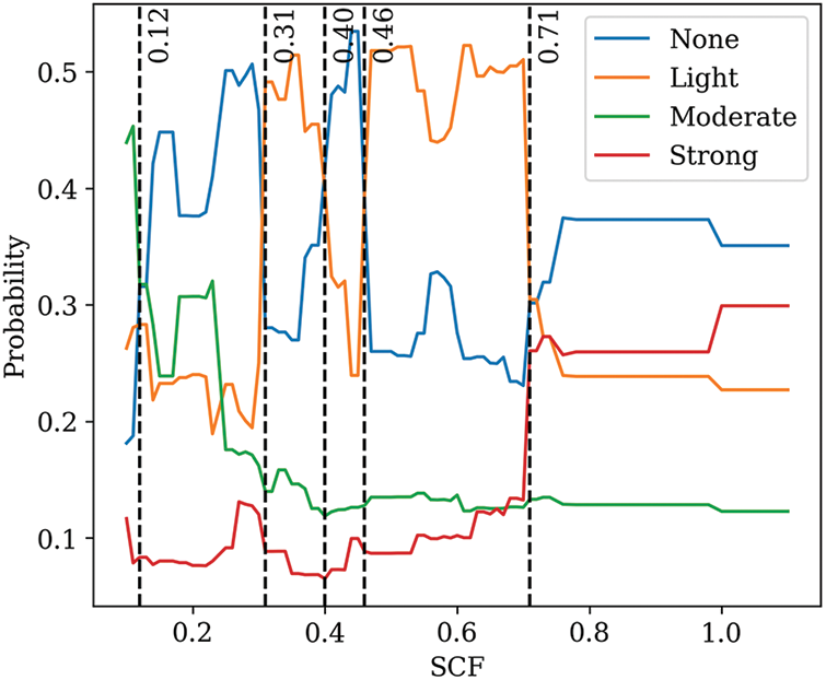
Figure 13: Impact of SCF in predicting the intensity of rock bursts

Overall, the relation between SCF and the risk of rock burst in this study is complex. SCF is a dimensionless quantity that describes how much the stress at a particular point is concentrated relative to the nominal stress. It is defined as the ratio of the maximum stress at a point to the nominal stress. The above analysis unveils that a lower SCF may induce a moderate risk of rock burst, while a higher SCF can eliminate the risk of rock burst, which is based on the data of this study.

Fig. 14 illustrates the impact of the elastic strain energy index (Wet) in predicting the intensity of rock burst. The factor Wet has a significant impact on ‘None’, ‘Light’, and ‘Moderate’ intensities of rock burst. When the value of Wet is greater than 0.81 but less than 1.73, the rock is at moderate risk of rock burst; when the value of Wet is greater than 1.73 but less than 3.60, the rock is at none risk of rock burst; when the value of Wet is greater than 3.60 but less than 10.0, the rock is at light risk of rock burst. Additionally, we also find that there is no risk of occurring rock bursts with strong intensity as the Wet changes from 0.81 to 10.0.

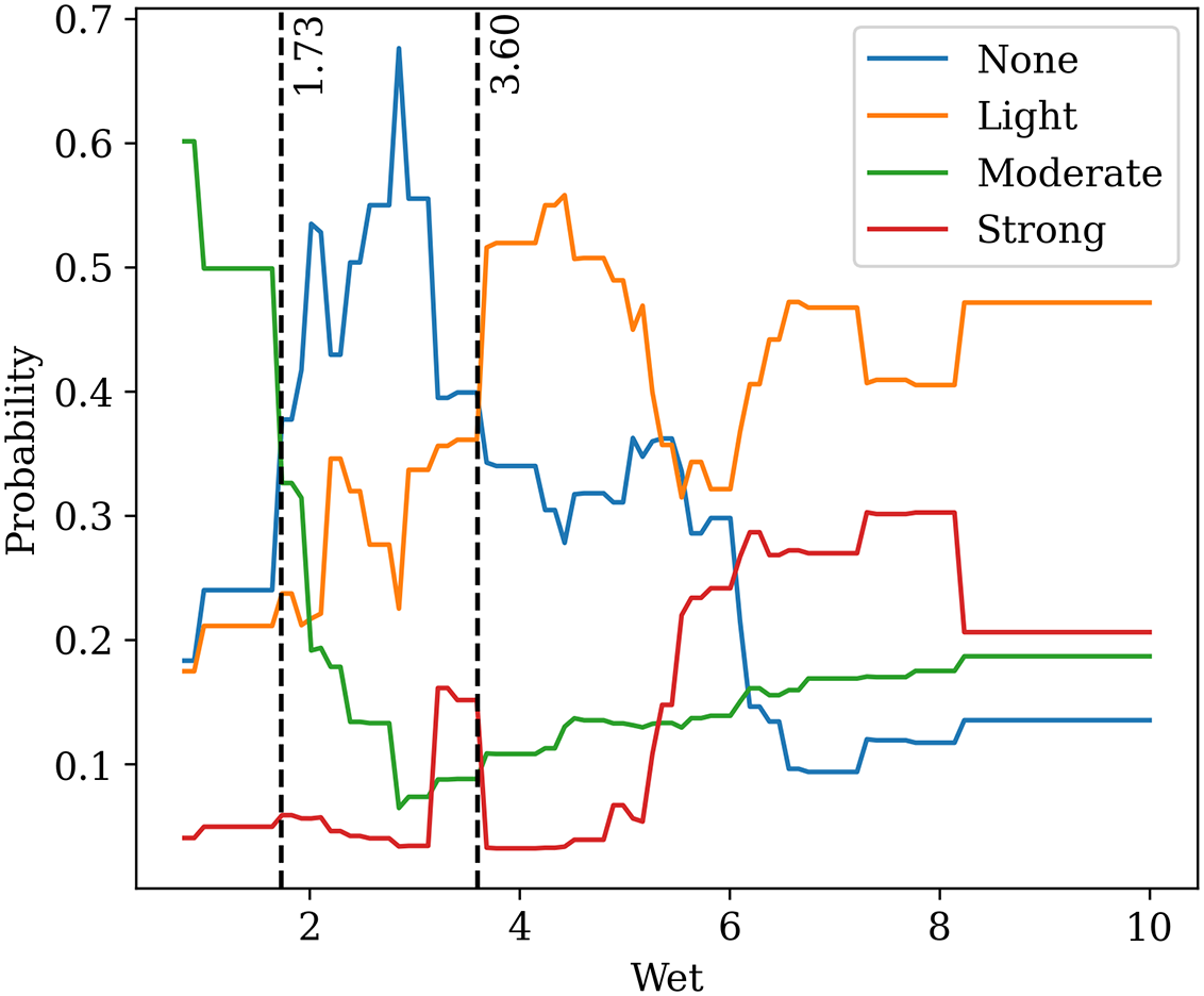
Figure 14: Impact of Wet in predicting the intensity of rock burst

Overall, the risk of a rock burst is sensitive to the change of Wet as a lower or a higher Wet can induce the occurrence of a rock burst. The Wet refers to the energy stored within a material when it undergoes deformation under elastic conditions. In the context of rocks, it's related to the energy accumulated as a result of the deformation of rock masses due to stress, which can occur over a long period. High Wet values may indicate that the rock mass has undergone significant deformation, and it could be at a higher risk of experiencing a rock burst.

5  Limitations and Outlook

Although this study develops a high-accuracy LightGBM model to predict the intensity of rock bursts, some limitations should be highlighted here. The first one is that the used dataset only includes a few factors of rock mechanical properties. Other factors such as the rock integrity coefficient and geometric size of the excavation profile are also essential for identifying the intensity of the rock burst. On the other hand, most rock burst cases in this study were collected from China, which may render the established model prone to site-specific biases. Thus, incorporating additional rock burst scenarios, such as from regions like Poland, would enrich the diversity and representativeness of the current dataset.

Moreover, the size of the dataset is limited, only 268 samples were used to build the LightGBM model. Based on these, future research avenues can focus on collecting new data that comprises more factors influencing the intensity of rock bursts. Likewise, some data augmentation techniques, such as generative adversarial network [42,43], variational autoencoder [44,45], and diffusion probabilistic model [46], can also be applied to increase the size of the raw dataset.

6  Conclusions

This study designs a tree-based LightGBM that is optimized by two population-based algorithms: the coati optimization algorithm (COA) and the pelican optimization algorithm (POA). A dataset including 268 rock burst scenarios is used to build the LightGBM model. 80% of the entire dataset is used to train the LighGBM model, while the rest 20% is used to evaluate the model’s performance. Lastly, the partial dependence plot (PDP) is used to identify the importance of factors in predicting the intensity of rock bursts. The main conclusions can be drawn as follows:

(1) The optimization algorithms, i.e., COA and POA, evolve with excellent and ideal running time, diversities, and exploitation and exploration rates. The ‘COA-60’ captured the optimal hyperparameters of the LighGBM model, which are 0.3 and 17 for the colsample_bytree and min_child_samplesi, respectively.

(2) The LightGBM model yielded good performance in predicting the intensity of rock bursts. Its predictive accuracy on the training set is 0.972 and on the testing set is 0.944.

(3) The sensitivity analysis unveiled that the risk of rock burst is sensitive to three factors: uniaxial compressive strength (σc), stress concentration factor (SCF), and elastic strain energy index (Wet). Moreover, this study discussed the particular impact of each factor on the risk of rock bursts, which helps identify the risk of rock bursts in real-world underground engineering.

Acknowledgement: The authors would like to appreciate the Faculty of Engineering, Universiti Malaya, and the facilities provided which enabled the study to be carried out.

Funding Statement: The authors received no specific funding for this study.

Author Contributions: The authors confirm their contribution to the paper as follows: study conception and design: K.W. and B.H.; data collection: K.W. and B.H.; analysis and interpretation of results: K.W., B.H., P.S., and J.Z.; draft manuscript preparation: K.W., B.H., P.S., and J.Z. All authors reviewed the results and approved the final version of the manuscript.

Availability of Data and Materials: Data will be made available on request.

Conflicts of Interest: The authors declare that they have no conflicts of interest to report regarding the present study.

References

1. Xue, Y., Li, Z., Li, S., Qiu, D., Tao, Y. et al. (2019). Prediction of rock burst in underground caverns based on rough set and extensible comprehensive evaluation. Bulletin of Engineering Geology and the Environment, 78, 417–429. https://doi.org/10.1007/s10064-017-1117-1 [Google Scholar] [CrossRef]

2. Jia, Q., Wu, L., Li, B., Chen, C., Peng, Y. (2019). The comprehensive prediction model of rockburst tendency in tunnel based on optimized unascertained measure theory. Geotechnical and Geological Engineering, 37, 3399–3411. https://doi.org/10.1007/s10706-019-00854-9 [Google Scholar] [CrossRef]

3. Zhang, W., Ma, N., Ma, J., Li, C., Ren, J. (2020). Mechanism of rock burst revealed by numerical simulation and energy calculation. Shock and Vibration, 2020, 1–15. https://doi.org/10.1155/2020/8862849 [Google Scholar] [CrossRef]

4. Zhang, W., Feng, J., Ma, J., Shi, J. (2022). The revealed mechanism of rock burst based on an innovative calculation method of rock mass released energy. International Journal of Environmental Research and Public Health, 19, 1–12. https://doi.org/10.3390/ijerph192416636 [Google Scholar] [PubMed] [CrossRef]

5. Zhou, J., Zhang, Y., Li, C., He, H., Li, X. (2024). Rockburst prediction and prevention in underground space excavation. Underground Space, 14, 70–98. [Google Scholar]

6. Zhou, J., Li, E., Wang, M., Chen, X., Shi, X. et al. (2019). Feasibility of stochastic gradient boosting approach for evaluating seismic liquefaction potential based on SPT and CPT case histories. Journal of Performance of Constructed Facilities, 33, 1–10. https://doi.org/10.1061/(asce)cf.1943-5509.0001292 [Google Scholar] [CrossRef]

7. Askaripour, M., Saeidi, A., Rouleau, A., Mercier-Langevin, P. (2022). Rockburst in underground excavations: A review of mechanism, classification, and prediction methods. Underground Space, 7, 577–607. https://doi.org/10.1016/j.undsp.2021.11.008 [Google Scholar] [CrossRef]

8. Xue, Y., Bai, C., Qiu, D., Kong, F., Li, Z. (2020). Predicting rockburst with database using particle swarm optimization and extreme learning machine. Tunnelling and Underground Space Technology, 98, 103287. https://doi.org/10.1016/j.tust.2020.103287 [Google Scholar] [CrossRef]

9. Liu, R., Ye, Y., Hu, N., Chen, H., Wang, X. (2019). Classified prediction model of rockburst using rough sets-normal cloud. Neural Computing and Applications, 31, 8185–8193. https://doi.org/10.1007/s00521-018-3859-5 [Google Scholar] [CrossRef]

10. Liu, H., Zhao, G., Xiao, P., Yin, Y. (2023). Ensemble tree model for long-term rockburst prediction in incomplete datasets. Minerals, 13, 1–18. https://doi.org/10.3390/min13010103 [Google Scholar] [CrossRef]

11. Qiu, Y., Zhou, J. (2023). Short-term rockburst prediction in underground project: Insights from an explainable and interpretable ensemble learning model. Acta Geotechnica, 18, 6655–6685. https://doi.org/10.1007/s11440-023-01988-0 [Google Scholar] [CrossRef]

12. Li, M., Li, K., Qin, Q. (2023). A rockburst prediction model based on extreme learning machine with improved harris hawks optimization and its application. Tunnelling and Underground Space Technology, 134, 104978. https://doi.org/10.1016/j.tust.2022.104978 [Google Scholar] [CrossRef]

13. Qiu, D., Li, X., Xue, Y., Fu, K., Zhang, W. et al. (2023). Analysis and prediction of rockburst intensity using improved D-S evidence theory based on multiple machine learning algorithms. Tunnelling and Underground Space Technology, 140, 105331. https://doi.org/10.1016/j.tust.2023.105331 [Google Scholar] [CrossRef]

14. Zhou, J., Li, X., Mitri, H. S. (2016). Classification of rockburst in underground projects: Comparison of ten supervised learning methods. Journal of Computing in Civil Engineering, 30, 1–19. https://doi.org/10.1061/(asce)cp.1943-5487.0000553 [Google Scholar] [CrossRef]

15. Li, D., Liu, Z., Armaghani, D. J., Xiao, P., Zhou, J. (2022). Novel ensemble intelligence methodologies for rockburst assessment in complex and variable environments. Scientific Reports, 12, 1–23. https://doi.org/10.1038/s41598-022-05594-0 [Google Scholar] [PubMed] [CrossRef]

16. Xu, G., Li, K., Li, M., Qin, Q., Yue, R. (2022). Rockburst intensity level prediction method based on FA-SSA-PNN model. Energies, 15, 1–19. https://doi.org/10.3390/en15145016 [Google Scholar] [CrossRef]

17. Liang, W., Sari, A., Zhao, G., McKinnon, S. D., Wu, H. (2020). Short-term rockburst risk prediction using ensemble learning methods. Natural Hazards, 104, 1923–1946. https://doi.org/10.1007/s11069-020-04255-7 [Google Scholar] [CrossRef]

18. Kadkhodaei, M. H., Ghasemi, E., Sari, M. (2022). Stochastic assessment of rockburst potential in underground spaces using monte carlo simulation. Environment Earth Science, 81, 1–15. https://doi.org/10.1007/s12665-022-10561-z [Google Scholar] [CrossRef]

19. Zhou, J., Li, X., Mitri, H. S. (2016). Classification of rockburst in underground projects: Comparison of ten supervised learning methods. Journal of Comput in Civil Engineering, 30, 4016003. [Google Scholar]

20. Pu, Y., Apel, D. B., Xu, H. (2019). Rockburst prediction in kimberlite with unsupervised learning method and support vector classifier. Tunnelling and Underground Space Technology, 90, 12–18. https://doi.org/10.1016/j.tust.2019.04.019 [Google Scholar] [CrossRef]

21. Wu, S., Wu, Z., Zhang, C. (2019). Rock burst prediction probability model based on case analysis. Tunnelling and Underground Space Technology, 93, 103069. https://doi.org/10.1016/j.tust.2019.103069 [Google Scholar] [CrossRef]

22. Zhou, J., Li, X., Shi, X. (2012). Long-term prediction model of rockburst in underground openings using heuristic algorithms and support vector machines. Safety Science, 50, 629–644. https://doi.org/10.1016/j.ssci.2011.08.065 [Google Scholar] [CrossRef]

23. Martin, C. D., Kaiser, P. K., McCreath, D. R. (1999). Hoek-brown parameters for predicting the depth of brittle failure around tunnels. Canadian Geotechnical Journal, 36, 136–151. https://doi.org/10.1139/t98-072 [Google Scholar] [CrossRef]

24. Liu, Z., Armaghani, D. J., Fakharian, P., Li, D., Ulrikh, D. V. et al. (2022). Rock strength estimation using several tree-based ML techniques. Computer Modeling in Engineering & Sciences, 133, 799–824. https://doi.org/10.32604/cmes.2022.021165 [Google Scholar] [CrossRef]

25. Wickham, H., Stryjewski, L. (2011). 40 years of boxplots. Statistician, 1–17. [Google Scholar]

26. Sim, C. H., Gan, F. F., Chang, T. C. (2005). Outlier labeling with boxplot procedures. Journal of the American Statistical Association, 100, 642–652. https://doi.org/10.1198/016214504000001466 [Google Scholar] [CrossRef]

27. Smiti, A. (2020). A critical overview of outlier detection methods. Computer Science Review, 38, 100306. https://doi.org/10.1016/j.cosrev.2020.100306 [Google Scholar] [CrossRef]

28. Bouayad, D., Emeriault, F. (2017). Modeling the relationship between ground surface settlements induced by shield tunneling and the operational and geological parameters based on the hybrid PCA/ANFIS method. Tunnelling and Underground Space Technology, 68, 142–152. https://doi.org/10.1016/j.tust.2017.03.011 [Google Scholar] [CrossRef]

29. Nguyen, M. D., Pham, B. T., Ho, L. S., Ly, H. B., Le, T. T. et al. (2020). Soft-computing techniques for prediction of soils consolidation coefficient. Catena, 195, 104802. https://doi.org/10.1016/j.catena.2020.104802 [Google Scholar] [CrossRef]

30. Ke, G., Meng, Q., Finley, T., Wang, T., Chen, W. et al. (2017). LightGBM: A highly efficient gradient boosting decision tree. In: Advances in neural information processing systems 2017, pp. 3147–3155. [Google Scholar]

31. Yari, M., He, B., Armaghani, D. J., Abbasi, P., Mohamad, E. T. (2023). A novel ensemble machine learning model to predict mine blasting-induced rock fragmentation. Bulletin of Engineering Geology and the Environment, 82, 1–16. https://doi.org/10.1007/s10064-023-03138-y [Google Scholar] [CrossRef]

32. Pedregosa, F., Varoquaux, G., Gramfort, A., Michel, V., Thirion, B. et al. (2011). Scikit-learn: Machine learning in Python. Journal of Machine Learning Research, 12, 2825–2830. [Google Scholar]

33. Dehghani, M., Montazeri, Z., Trojovská, E., Trojovský, P. (2023). Coati optimization algorithm: A new bio-inspired metaheuristic algorithm for solving optimization problems. Knowledge-Based Systems, 259, 110011. https://doi.org/10.1016/j.knosys.2022.110011 [Google Scholar] [CrossRef]

34. Trojovský, P., Dehghani, M. (2022). Pelican optimization algorithm: A novel nature-inspired algorithm for engineering applications. Sensors, 22, 1–34. https://doi.org/10.3390/s22030855 [Google Scholar] [PubMed] [CrossRef]

35. Cully, A., Demiris, Y. (2018). Quality and diversity optimization: A unifying modular framework. IEEE Transactions on Evolutionary Computation, 22, 245–259. https://doi.org/10.1109/TEVC.2017.2704781 [Google Scholar] [CrossRef]

36. Črepinšek, M., Liu, S. H., Mernik, M. (2013). Exploration and exploitation in evolutionary algorithms. ACM Computing Surveys, 45, 1–33. https://doi.org/10.1145/2480741.2480752 [Google Scholar] [CrossRef]

37. Goutte, C., Gaussier, E. (2005). A probabilistic interpretation of precision, recall and F-score. European Conference on Information Retrieval, pp. 345–359. Santiago de Compostela, Spain. [Google Scholar]

38. Li, D., Liu, Z., Armaghani, D. J., Xiao, P., Zhou, J. (2022). Novel ensemble tree solution for rockburst prediction using deep forest. Mathematics, 10, 1–23. https://doi.org/10.3390/math10050787 [Google Scholar] [CrossRef]

39. Qiu, Y., Zhou, J. (2023). Short-term rockburst damage assessment in burst-prone mines: An explainable XGBOOST hybrid model with SCSO algorithm. Rock Mechanics and Rock Engineering, 1–26. https://doi.org/10.1007/s00603-023-03522-w [Google Scholar] [CrossRef]

40. Ly, H. B., Pham, B. T. (2020). Prediction of shear strength of soil using direct shear test and support vector machine model. The Open Construction & Building Technology Journal, 14, 268–277. https://doi.org/10.2174/1874836802014010268 [Google Scholar] [CrossRef]

41. Wang, J., Yan, W., Wan, Z., Wang, Y., Lv, J. et al. (2020). Prediction of permeability using random forest and genetic algorithm model. Computer Modeling in Engineering & Sciences, 125, 1135–1157. https://doi.org/10.32604/cmes.2020.014313 [Google Scholar] [CrossRef]

42. Habibi, O., Chemmakha, M., Lazaar, M. (2023). Imbalanced tabular data modelization using CTGAN and machine learning to improve IoT botnet attacks detection. Engineering Applications of Artificial Intelligence, 118, 105669. https://doi.org/10.1016/j.engappai.2022.105669 [Google Scholar] [CrossRef]

43. Xu, L., Skoularidou, M., Cuesta-Infante, A., Veeramachaneni, K. (2019). Modeling tabular data using conditional GAN. In: Advances in neural information processing systems. [Google Scholar]

44. Kingma, D. P., Welling, M. (2014). Auto-encoding variational bayes. 2nd International Conference Learning Representations, pp. 1–14. [Google Scholar]

45. Kingma, D. P., Welling, M. (2019). An introduction to variational autoencoders. Foundations and Trends in Machine Learning, 12, 307–392. https://doi.org/10.1561/2200000056 [Google Scholar] [CrossRef]

46. Ho, J., Jain, A., Abbeel, P. (2020). Denoising diffusion probabilistic models. In: Advances in neural information processing systems, pp. 1–12. [Google Scholar]