Reduced-Order Observer-Based LQR Controller Design for Rotary Inverted Pendulum

1  Introduction

The Rotary Inverted Pendulum (RIP), also known as the Furuta Pendulum, has been extensively studied by researchers since its introduction in 1992 [1,2]. The RIP system, characterized by high instability, multivariate, nonlinear, and underactuated properties, is regarded as an ideal benchmark system for the training and validation of new control strategies in the field of engineering control. The study of dynamic modelling and equilibrium state control algorithms for the RIP systems is crucial in advanced technological sectors, especially in aerospace industry. Moreover, the progress in this field has found extensive application in daily life, as demonstrated by the steady-state control mechanisms used in Segway [3], bipedal robots [4], and skyscrapers [5]. Furthermore, the control principle of cranes [6] and offshore drilling platforms [7] share similarities with the model when the pendulum is suspended.

In fact, these mechanical systems exemplify a category of attitude control challenges that essential goal is to drive the arm in following a prescribed time-varying trajectory while keeping the pendulum balanced near a stable upright position. To achieve this, numerous linear and nonlinear controller synthesis methods have attracted significant interest and research attention. Among them, proportional-integral-derivative (PID) control or its hybrid variants are frequently used controllers [8,9], due to its simplistic structure, cost-effectiveness, and ease of implementation in hardware. Ideally, the performance of controlled dynamical systems should be optimal. However, determining the optimal control gain to efficiently suppress uncertain nonlinearities using the system dynamics model is challenging when designing a PID controller. Moreover, the PID controller is designed for linear applications without considering saturation nonlinearity, which may result in performance degradation or even instability in certain instances. In recent years, it has been found that the peculiarities of fractional calculus in mathematics provide an extension to the traditional PID method. Dwivedi et al. [10] was the first to design and test a fractional-order PID (FOPID) controller on RIP, and the saturation effect when the control input is saturated was mitigated by combining the FOPID controller with an anti-windup technique [11]. Linear quadratic regulation (LQR) is another commonly used optimal control method, which is based on minimizing a quadratic performance criterion that encapsulates state and control input variations. In references [12–14], the LQR controller was utilized to stabilize the attitude dynamics of RIP in an upright posture. Although LQR is optimal, it lacks robustness against parametric uncertainties. Therefore, hybrid versions of LQR, which incorporate additional control strategies, filters or observers, were employed to address this deficiency while ensuring robustness and optimal performance. For instance, the linear quadratic gaussian (LQG) controller, which combines a Kalman filter observer and LQR, was presented in [15,16]. Hybrid control, formulated in [17], integrates backstepping and LQR. Additionally, in [18], the combination of passivity-based control and LQR was analyzed, designed and implemented on RIP.

Recent advancements in artificial intelligence (AI) and evolutionary computational techniques, collectively referred to as intelligent computational techniques, have introduced innovative solutions for controlling RIP systems. AI has gained popularity in clustering random complex matrices [19] and graphs [20]. There has been a recent surge in the development of an intelligent optimal control approach that integrates the adaptive features of intelligent computation into traditional linear control frameworks. Rather than manually tuning LQR, the state weighting matrices in [21,22] have been dynamically adjusted based on secant hyperbolic functions (SHFs) or optimized using particle swarm optimization (PSO) algorithms. Additionally, LQR controllers with fuzzy tuning have improved robustness in practical applications [23]. Consequently, the retrofitted LQR has demonstrated superior control outcomes. To fully exploit the benefits of intelligent algorithms and optimal control, some researchers have focused on associating LQR with a neural network (NN) for improving system response. In [24,25], LQR determines the stability of the IP system around arbitrary equilibrium points, while the NN control improves transient performance when deviations occur from an intended point and suppresses system bias.

In the aforementioned works, system models and state variables are pivotal in deriving optimal control laws or strategies to achieve the desired response and performance. However, many physical states of the system are either unmeasurable or extremely difficult to measure using sensors. Moreover, sensors are susceptible to noise interference, resulting in the acquisition of inaccurate measurements. A review of the existing literature shows that although a number of well-known control strategies, including neural NN-based system identification [26,27], fuzzy control (FC) [13,23], sliding mode control (SMC) [28], model-free control (MFC) [29], and hybrids of these, can mitigate the inherent problems of model-based control, but each has its own limitations. For example, NN often requires extensive experimental datasets for effective training and testing; to ensure robustness, FC relies on intricate qualitative logic rules derived from the relevant experience of the operator or designer; while SMC accelerates system stabilization, but often leads to undesirable oscillation. Additionally, in practical control engineering systems, the simplicity of control algorithms is highly desired along with the achievement of control objectives.

Motivated by the aforementioned challenges and inspired by the observer-based control approach detailed in references [30–33], this study focuses on the stabilizing and tracking control problems for RIP systems using a reduced-order observer feedback within a LQR control framework. The contributions of this study are outlined as follows:

(1) The RIP was analyzed and modeled using Newton-Euler and Lagrange equations. Additionally, the controllability and observability of the system were determined, and the feedback gain matrix was evaluated.

(2) A reduced-order observer was proposed to reconstruct the unmeasured system states and showed excellent robustness to low-amplitude, high-frequency disturbances by eliminating the differential term.

The remainder of this paper is organized as follows: Section 2 presents the mathematical model and linearization of the RIP system. In Section 3, the design of the controller and reduced-order observer is introduced. In Section 4, simulations and experiments are given, respectively. Finally, the main conclusions are presented in Section 5.

2  Dynamic Model of RIP

The RIP system comprises an unactuated pendulum that freely rotates in a vertical plane, perpendicular to the tip of a horizontally rotating arm driven by a direct current (DC) motor. The system is characterized by two degrees of mechanical freedom and a single control input, as illustrated in Fig. 1. Angle sensors are employed to detect the angle at which the pendulum deviates from equilibrium. The rotary arm and a parallel Z-axis are depicted in Fig. 1, with the inertial earth-fixed reference frame labelled as O-XYZ and the arm-fixed reference frame as O′-X′Y′Z′.

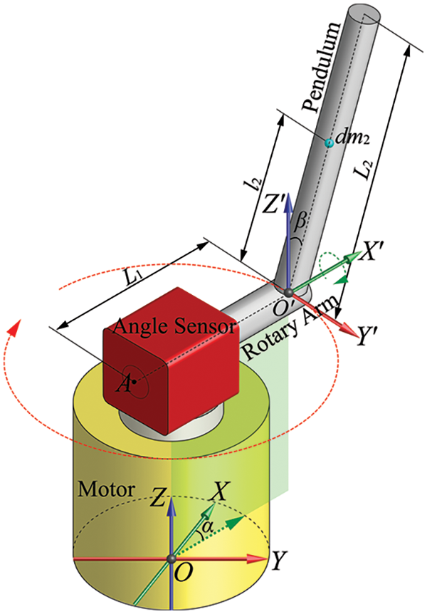
Figure 1: The RIP with reference frames

It is assumed that the pendulum is homogeneous. The rotary arm and pendulum have masses M1 and M2, respectively. To calculate a microelement of mass represented as dm2, situated at a distance l2 from point O′ on the pendulum, as follows:

dm2=ρ2dl2=M2L2dl2,(1)

where ρ2 represents the pendulum density, while dl2 refers to the microelement length. Fig. 2 provides a visualization of the pendulum’s projection onto the XOY plane. From this, the coordinates of dm2 in the O-XYZ frame can be determined as

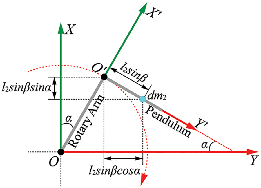
Figure 2: The pendulum projection into the XOY plane

{X=L1cos⁡α−l2sin⁡βcos⁡α,Y=L1sin⁡α+l2sin⁡βcos⁡α,Z=l2cos⁡β.(2)

From Eqs. (1) and (2), the kinetic energy ek of the microelement is given by

ek=12dm2v22=M22L2[(dXdt)2+(dYdt)2+(dZdt)2]dl2,(3)

where v2 denotes the microelement’s velocity. While, the kinetic energy of the whole pendulum Ek2 can be determined as

Ek2=∫0L2ekdl2=L12M2α˙22+L12M2α˙2(sin⁡β)26+L22M2β˙26+L1L2M2α˙β˙cos⁡β2.(4)

The kinetic energy Ek1 of the rotary arm can be calculated using Koening’s theorem as follows:

Ek1=J1ω122=M1L12α˙26.(5)

In this equation, J1=13M1L12 represents the rotary arm’s moment of inertia about the fixed Z-axis. Consequently, the kinetic energy of RIP is ascertained by Eqs. (4) and (5), that is

Ek=Ek1+Ek2=M1L12α˙26+L12M2α˙22+L12M2α˙2(sin⁡β)26+L22M2β˙26+L1L2M2α˙β˙cos⁡β2.(6)

Define the plane X′O′Y′ as the reference plane. Around upright equilibrium, the potential energy Ep of the pendulum is

Ep=M2gL2cos⁡β2.(7)

Equations describing rotary arm and pendulum motions with respect to DC motor voltage are obtained by the Euler-Lagrange equation

∂2L∂t∂qi˙−∂L∂qi=Qi.(8)

The Lagrangian function, L, can be inferred from Eqs. (6) and (7), which can be represented as L=Ek−Ep. In this case, the generalized coordinates are defined as qi=[α(t),β(t)]T. Qi represents the non-potential forces of generalization that are exerted on the system in relation to the generalized coordinates, as follows:

{Q1=τ−Brα˙,Q2=−Bpβ˙,(9)

where Br is the viscous friction coefficient of the motor, and Bp is the viscous damping coefficient of the pendulum [14,34]. The net output torque of the DC motor acting on the load is described by

τ=KtRm(Vm−Kmα˙).(10)

In which, Kt is torque constant. Rm is the motor armature resistance. Vm is the armature input voltage. Km is the motor-back EMF constant. Substituting Eqs. (6), (7), (9) and (10) into Eq. (8), the nonlinear dynamics model for the RIP system can be derived as follows:

{[L12M13+L12M2+L12M2(sin⁡β)23]α¨+(KtKmRm+Br)α˙+2L12M2sin⁡βcos⁡β3α˙β˙+L1L2M2cos⁡β2β¨−L1L1M2sin⁡β2β˙2=KtVmRm,L1L2M2cos⁡β2α¨−L12M2cos⁡βsin⁡β3α2+L22M23β¨+Bpβ˙−M2gL2sin⁡β2=0.(11)

The state variables are defined as x=[x1 x2 x3 x4]T=[α β α˙ β˙]T. The upright equilibrium point can be expressed as xf=[x1f x2f x3f x4f]T=[θ 0 0 0]T,

where θ∈[0,2π] represents the desired arm angle. The system can be linearly approximated by resolving the Taylor expansion of Eq. (11) around xf. Disregarding the higher-order infinitesimal terms, the state-space expression can be derived as

[x˙1x˙2x˙3x˙4]⏞x˙=[001000010a32a33a340a42a43a44]⏞A[x1x2x3x4]⏞x+[00b31b41]⏞BVm,(12)

[y1y2]⏞y=[10000100]⏞C[x1x2x3x4]⏞x+[00]⏞DVm,(13)

where A, B, C and D represent the linearized state-space matrices, and y represents the measured output. Matrices A and B contain the following elements:

a32=−9M2gL1(4M1+3M2),=a33=−12(KtKm+BrRm)L12Rm(4M1+3M2),=a34=18BpL1L2(4M1+3M2),a42=6g(M1+3M2)L2(4M1+3M2),=a43=18(KtKm+BrRm)L1L2Rm(4M1+3M2),=a44=−12B2(M1+3M2)L22M2(4M1+3M2),b31=12KtL12Rm(4M1+3M2),=b41=−18KtRmL1L2(4M1+3M2).

3  Controller and Reduced-Order Observer Design

The eigenvalues of matrix A clearly indicate that the RIP is an unstable system of type I, and xf is an unstable equilibrium point. This implies that if the state variables x deviate from xf, the single input multiple output (SIMO) system will not return to xf without external input. Therefore, to progressively stabilize the system, it is necessary to design a suitable armature input voltage, i.e., Vm, which alters the properties of xf.

3.1 LQR-Based Controller Design

As stated in Eqs. (12) and (13), let u(t)=Vm(t), the state-space equation can be rewritten as

In a closed-loop control system, the system input u(t) is a function of the state variables. The system can be considered controllable and observable if and only if both matrices Co and Ob have full ranks, where

Co=[B, AB, A2B, A3B],Ob=[C, CA, CA2, CA3]T.

Given the parameters listed in Table 1, matrices A, B and C can be calculated. Obviously, both matrices have a rank of 4, indicating controllability and observability of the dynamical system described by Eqs. (14) and (15).

For the Type I RIP system, its inherent underdriven characteristics dictate that x2f=x3f=x4f=0 is the unique equilibrium point. Although the RIP system is controllable, and the state variables x2, x3 and x4 can reach the desired values, it does not necessarily imply that they can be stabilized at those values. In fact, the pendulum remains unstable as long as x2, x3 or x4 are non-zero. Unlike the other variables, x1 can be stabilized at any desired angle under the influence of the input signal u(t). To achieve the target equilibrium point, we utilize the state feedback control scheme depicted in Fig. 3, which can be expressed as

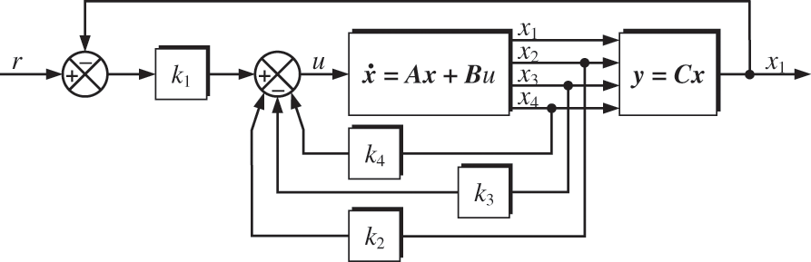
Figure 3: State feedback control scheme

u(t)=k1(r−x1)−[k2k3k4][x2x3x4]=−Kx(t)+k1r(t),(16)

where K is the state feedback gain (SFG) matrix, k1 is the SFG of x1, r(t) is the reference input of x1, i.e., the desired arm angle.

The u(t) is designed to perform two functions: adjusting the arm’s equilibrium point and asymptotically stabilising it. The system dynamics can be determined from Eqs. (16) and (14) as x˙(t)=(A−BK)x(t)+Bk1r(t). Assuming that the system output y=x1, when t→∞, the RIP is asymptotically stabilized by u(t), while y(∞)→r(∞)=r(t). Let e(t)=x(t)−x(∞), then we have e˙(t)=x˙(t)−x˙(∞), and error dynamics can be described as

{e˙(t)=x˙(t)−x˙(∞)=(A−BK)e(t),ue(t)=u(t)−u(∞)=−Ke(t).(17)

The state matrix of closed-loop control systems can be expressed as Acl=(A−BK). The comprehensive performance index (CPI) is an effective tool for analyzing and designing control systems, providing a means to quantify the performance of the system. In general, the system that attains an extreme (usually minimal) value of the CPI through system parameter adjustments is deemed optimal. If the system’s CPI is denoted by J, the objective here is to find a suitable K that minimizes J for any given initial condition e(0), while ensuring that all eigen roots of Acl possess negative real parts. Eq. (18) is the expression of the LQR, which is a commonly used CPI for linear control systems described by state variables.

J=∫0∞(eTQe+ueTRue)dt=∫0∞[eT(Q+KTRK)e]dt,(18)

where Q and R are positive definite square weight matrices used to scale the relative contributions of quadratic terms eTQe and ueTRue, respectively. Suppose that P is a matrix, which satisfies (eTPe)′=−eT(Q+KTRK)e, with t→∞, x(t)→x(∞)=xf, and e(t)→0. The algebraic form of Eq. (18) (i.e., the minimum of J) can be obtained as

J=−∫0∞d(eTPe)dtdt=−eTPe|0∞=e(0)TPe(0).(19)

Moreover, it is worthwhile to note that along with Eq. (17) we also have (eTPe)′=eT(AclTP+PAcl)e. In view of the above analysis, Eq. (19) is valid if pending matrix P can make

−(Q+KTRK)=(AclTP+PAcl).(20)

The Riccati equation [14,22,24] can be solved to yield the matrix P. Then, this matrix can be substituted into Eq. (20) to determine the gain matrix K, expressed as

K=R−1BTP.(21)

3.2 Reduced-Order Observer Design

Due to the installation environment or other factors, there might be a need for an observer to estimate states that cannot be directly measured. In this project, a reduced-order observer is constructed specifically to estimate states x3 and x4. By dividing x into a measurable xa and an unmeasurable xb, Eqs. (12) and (13) can be rewritten as

[x˙a(t)x˙b(t)]=[AaaAabAbaAbb][xa(t)xb(t)]+[BaBb]u(t),(22)

y(t)=[I(2)0(2)][xa(t)xb(t)],(23)

where I(2) represents a 2-dimensional identity matrix. Further expanded and organized to get

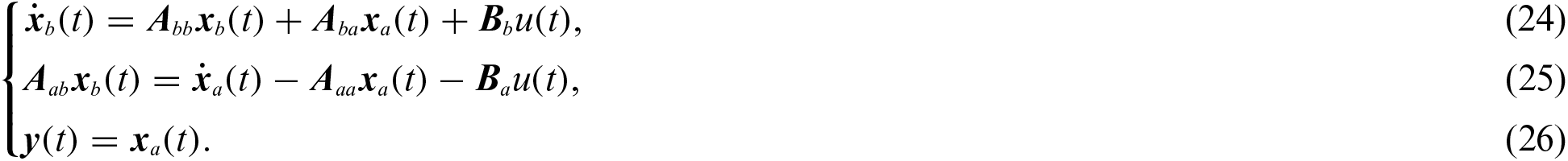
The unmeasurable states can be interpreted through Eqs. (24) and (25), which serve as the dynamic differential equation and output equation, respectively. By utilizing the design methodology of the Luenberger full-order state observer and using error feedback between the measured and estimated output, a reduced-order observer for xb can be constructed as

x~˙b=Abbx~b+Abaxa+Bbu+L(Aabxb−Aabx~b)=(Abb−LAab)x~b+Abaxa+Bbu+L(x˙a−Aaaxa−Bau),(27)

where L is the state observation gain matrix. It is essential to emphasize that xa must be differentiated to yield xb. Considering the sensitivity of the differentiation session to noise, it is wise to eliminate x˙a. Therefore, Eq. (27) can be rephrased as

x~˙b−Lx˙a=(Abb−LAab)x~b+(Aba−LAaa)xa+Bbu−LBau=(Abb−LAab)x~b+(Abb−LAab)Ly−(Abb−LAab)Ly+(Aba−LAaa)xa+Bbu−LBau=(Abb−LAab)(x~b−Ly)+[(Abb−LAab)L+Aba−LAaa]y+(Bb−LBa)u.(28)

Define

{xb−Lxa=xb−Ly=η,x~b−Lxa=x~b−Ly=η~,x~˙b−Lx˙a=η~˙,x~=[xax~b]=[yx~b],{A^=Abb−LAab,B^=A^L+Aba−LAaa,F^=Bb−LBa,C^=[0(2)I(2)],D^=[I(2)L].(29)

The reduced-order observer can be derived by substituting Eq. (29) for Eq. (28)

where the transformation relation from η~ to x~ is presented in Eq. (32). By virtue of

u=−[KaKb][xax~b]+k1r=−[KaKb][y~η~+Ly]+k1r=−(Kay+Kbη~+KbLy)+k1r,(33)

Eq. (30) can be further derived as

η~˙=(A^−F^Kb)η~+(B^−F^Ka−F^KbL)y+F^k1r.(34)

Define the observation error eb=xb−x~b, and subtract Eq. (27) from Eq. (24), we get

e˙b=x˙b−x~˙b=(Abb−LAab)eb=A^eb.(35)

It should be emphasized that the assumption of eb→0 implies the absence of model error, an impossibility in practical applications. The gain matrix L depends on the eigen-equation |λI−(Abb−LAab)|=0, and the eigenvalue λ is not unique. In general, λ should be chosen such that the observer exhibits the following characteristics: (a). it asymptotically stabilizes the observer, as indicated by Eq. (34); (b). it maintains eb within an acceptable range; (c). it ensures the rapid attenuation of eb is at least 2 to 5 times faster than that of xb. The substitution of Eq. (16) into Eq. (14) yields the following:

x˙=Ax−BKx~+Bk1r=Ax−BK{[xaxb]−[0eb]}+Bk1r=(A−BK)x+BKbeb+Bk1r.(36)

Combining Eqs. (35) and (36), we get

[x˙(t)e˙b(t)]=[(A−BK)BKb0(Abb−LAab)][x(t)eb(t)]+[Bk10]r(t).(37)

By analyzing the dynamic properties of xb and eb by simulation, λ can be selected, and then L will be obtained by pole placement method.

4  Simulation and Validation

All the parameter symbols and values used in RIP system modeling are summarized in Table 1.

4.1 Simulation

Using the values given in Table 1, the system state equation is

[x˙1x˙2x˙3x˙4]⏞x˙=[001000010−55.0963−6.2835−1.81590168.4091−6.2104−5.5506]⏞A[x1x2x3x4]⏞x+[00−18.3728−18.1591]⏞Bu.(38)

LQR controller performance is dependent on the choice of weight matrices Q and R. Here Q matrix is defined as Q=diag[q1,q2,q3,q4]

where q1,q2,q3,q4 are the weight coefficients of state variables x1 (arm angle), x2 (pendulum angle), x3 (arm velocity), x4 (pendulum velocity), respectively. The weight of control input is considered as R, which is a scalar. Larger weight coefficients will give the variables corresponding to them a greater weight in the CPI, thus giving them a faster convergence rate. In the literature, many different approaches exist for the choice of weight matrix, e.g., Bryson’s Rule. In this case, x1 and x2 are crucial, so q1 and q2 should be given a high weight. Conversely, q3 and q4 should be minimized because x3 and x4 are irrelevant. To test the effect of different weight matrices on controller performance, four groups of experiments are conducted using the same initial conditions as shown in Table 2, and the simulation results are shown in Fig. 4. Here, the area of the region formed by the state curve and the coordinate axes is calculated by ∫t0tfx1,22(t)dx, and the smaller the area, the faster convergence of the variables.

Figure 4: Simulation results of test experiments

The results show that x2 has a smaller order of magnitude than x1 and u, so increasing q2 has a limited effect on x2. As q2 grows, ∫t0tfu(t)dx, i.e., system energy consumption, increases as well. It is obvious that x1 is affected by q1, but in practical, a large q1 will cause the controller to be overly sensitive to x1, resulting in vibration in the system. Considering the above reasons and after numerous trials, the system performed satisfactorily with Q=diag[15,1,0.1,0.1] and R=1. Matrix K is solved by the LQR method, as described in Subsection 3.1.

K=[−3.8730,−49.9263,−2.0590,−3.630].

At this point, the system is asymptotically stabilized for any given initial state. Combining the controller Eq. (33), the reduced-order observer Eq. (30), and the transformation relation η~ to x~ Eq. (32), the control block diagram of the linear RIP system is shown in Fig. 5.

Figure 5: Control block diagram of the linear RIP system

The system, as shown in Figs. 6 and 7, exhibits asymptotic stability under the influence of u(t) for any initial state (in this case x(0)=[−π20 π45 0 0]T) and converges to an equilibrium point at xf=[0 0 0 0]. Fig. 6 illustrates an increase in x1 over time, within the interval t∈[0,0.32). Correspondingly, Fig. 7 displays x˙1, i.e., x3, which represents the rate of change of x1, and demonstrates x˙1>0 within the same time interval. However, when t≥0.32, x1 decreases over time, so x˙1<0. This negative rate of change manifests itself as an undershoot in Fig. 7 for the corresponding time interval. A similar relationship can be observed between x2 and x˙2, i.e., x4.

Figure 6: Angular response curves

Figure 7: Angular velocity response curves

Eq. (37) can be used to determine the response curve for any given initial condition. In addition, the convergence rate of eb as evident from Eq. (35) is influenced by the variation in L values, which are derived from the selection of different λ. Figs. 8 and 9 demonstrate observation of xb=[x3 x4]T and convergence of eb=[eb1 eb2]T, respectively, for the initial conditions of x(0)=[−π20 π45 1 1]T, eb(0)=[1 1] with

Figure 8: The observation and error dynamic of x3

Figure 9: The observation and error dynamic of x4

λ=[−22−24],L=[18.8890−10.9185−3.191821.0601].

The desired arm angle is defined as r(t)=π4[ε(t)−ε(t−10)]−π3ε(t−20)+5π6ε(t−30)−ε(t−40) for t∈[0,40],

where ε(t) represents the unit step signal. Figs. 10 and 11 illustrate the tracking result of α and the transition process of β as α varies, respectively. Analysis of these figures reveals that the forward overshooting of α is minimal. However, reverse overshooting occurs with 9.66% of the step amplitude before each step. It is not difficult to understand, because the arm rotates while taking into account the balance of the pendulum. Before the arm rotates, the pendulum must be diverted away from equilibrium along the arm rotation, and the pendulum is brought back to equilibrium as the arm rotates to the target position. Therefore, in order to divert the pendulum from the equilibrium position, the arm must be first rotated in the reverse direction by a specific angle before it is rotated to the desired position.

Figure 10: The desired signal and position tracking

Figure 11: Variation of β with α

4.2 Hardware Implementation and Validation

4.2.1 Experimental Setup

This method is validated with the Quanser QNET 2.0 RIP Board. Fig. 12 shows the system connection and front-end panel, which serve as the user interface for displaying state variation and controlling the application. The rotary arm is driven by a direct-drive 18 V brushed DC motor housed in a solid aluminum frame. Real-time variations in α and β are measured via rotary encoders commissioned at the motor’s shaft and pendulum’s pivot, respectively. The data samples are acquired at 200 Hz using the NI ELVIS II(+) data acquisition system. Using the block diagram tool in LabVIEW software, the customized control application is implemented as a visual instrument file, and the mathematical objects are acquired from its function palette. Control signals are serially transmitted to a Pulse-Width-Modulated (PWM) amplifier, which translates incoming signals into PWM commands and drives the DC motor.

Figure 12: The system connection and front-end panel

On this platform, two distinct experiments were conducted. The first experiment focused on examining the balance and disturbance rejection capabilities of the system following the pendulum’s swing up to the upright position. The second experiment concentrated on assessing the tracking control performance.

4.2.2 Balance Control

The experimental parameters used are consistent with those employed in the numerical simulation. Due to the manual erection and stabilization of the pendulum before each experiment, the initial conditions for activating balance control are random. Consequently, the data recording starts from the 5th second, as shown in Figs. 13 to 16. The controller’s capability to withstand mechanical vibration or process noise is evaluated by injecting sinusoidal and random signals of different frequencies and low-amplitude. In Fig. 13, the disturbance d1(t) is set as a random signal of 0.5 amplitude and 10 Hz frequency. The disturbance in Fig. 14 is determined by d2(t)=1.5sin⁡(2πt). The variables of α and β with time are shown in Figs. 15 and 16 for increasing the frequencies of d1(t) and d2(t) to 50, 100 and 200 Hz, respectively. As a result, it can be seen that the proposed controller maintains the RIP balance under low-amplitude disturbances. In addition, since differential terms are eliminated in the observer design, the controller’s sensitivity to disturbances decreases as its frequency increases. In several experiments, low-amplitude interference signals with frequencies greater than 50 Hz have no significant impact on this controller.

Figure 13: Disturbance d1(t) injection response

Figure 14: Disturbance d2(t) injection response

Figure 15: d1(t): Different frequencies are injected

Figure 16: d2(t): Different frequencies are injected

4.2.3 Tracking Control

The desired arm angle in the tracking control experiment is set to r(t)=π4[ε(t−5)−ε(t−15)]−π3ε(t−25)+4π9ε(t−35)−ε(t−45) for t∈[0,40],

where ε(t) is the unit step signal. The experimental results of tracking control are depicted in Fig. 17. Different from the simulation, it was observed that the step amplitude in the penultimate term is reduced from 5π6 to 4π9, expect for the step time delay of 5 s. The larger arm step amplitude necessitates a greater reverse overshoot prior to initiating the step. However, in this experiment, it was observed that the pendulum fails to return to equilibrium when the arm’s step amplitude exceeds 1.4 rad. This corresponds to a reverse overshoot that is approximately greater than 0.3 rad.

Figure 17: The tracking control results

5  Conclusion

This paper presents a reduced-order observer technique to estimate unmeasurable state variables and integrate these estimates into a full-state feedback controller for RIP. By combining estimation with measurement, a state feedback controller for RIP is designed based on the LQR technique. The conclusion is summarized as follows:

(1) Numerical simulations show that the theoretically established linear controller is able to stabilize the system rapidly.

(2) The balance control experiment confirmed that the RIP can be balanced below 50 Hz and tracked well below 1.4 rad.

In summary, the controller demonstrates proficient performance in balance stabilization and trajectory tracking, showcasing robustness against low-amplitude, high-frequency disturbances. These outcomes suggest that the proposed framework effectively contributes to both RIP balancing and tracking, offering novel theoretical insights and practical applications for industrial use.

While this study primarily addresses linear control theory, the precise control of mechanical systems warrants further exploration in the realm of nonlinear control algorithms. Consequently, future work will delve into nonlinear control algorithms for underactuated systems.

Acknowledgement: The authors wish to thank their colleagues for their suggestions to improve the quality of this article.

Funding Statement: This work is supported in part by the Youth Foundation of China University of Petroleum-Beijing at Karamay (under Grant No. XQZX20230038); the Karamay Innovative Talents Program (under Grant No. 20212022HJCXRC0005).

Author Contributions: The authors confirm contribution to the paper as follows: study conception and design: G. Gao, L. Xu; system analysis and modeling: T. Huang, X. Zhao; controller and observer design: G. Gao, T. Huang; platform construction and experimental design: X. Zhao; L. Huang; analysis and interpretation of results: L. Xu, L. Huang; draft manuscript preparation: G. Gao, T. Huang. All authors reviewed the results and approved the final version of the manuscript.

Availability of Data and Materials: The datasets generated and/or analyzed during this study are available from the corresponding author on reasonable request.

Conflicts of Interest: The authors declare that they have no conflicts of interest to report regarding the present study.

References

1. Furuta, K., Yamakita, M., Kobayashi, S. (1992). Swing-up control of inverted pendulum using pseudo-state feedback. Proceedings of the Institution of Mechanical Engineers, Part I: Journal of Systems and Control Engineering, 206(4), 263–269. [Google Scholar]

2. Hamza, M. F., Yap, H. J., Choudhury, I. A., Isa, A. I., Zimit, A. Y. et al. (2019). Current development on using rotary inverted pendulum as a benchmark for testing linear and nonlinear control algorithms. Mechanical Systems and Signal Processing, 116, 347–369. [Google Scholar]

3. Ch, R. P., Ch, R., Assaf, M., Narayan, S. V., Naicker, P. R. et al. (2022). Acceleration feedback controller processor design of a segway. 2022 IEEE 7th Southern Power Electronics Conference (SPEC), Nadi, Fiji, IEEE. [Google Scholar]

4. Li, Z., Zeng, J., Chen, S., Sreenath, K. (2023). Autonomous navigation of underactuated bipedal robots in height-constrained environments. The International Journal of Robotics Research, 42(8), 565–585. [Google Scholar]

5. Zhou, K., Zhang, J. W., Li, Q. S. (2022). Control performance of active tuned mass damper for mitigating wind-induced vibrations of a 600-m-tall skyscraper. Journal of Building Engineering, 45, 103646. [Google Scholar]

6. Sun, N., Fu, Y., Yang, T., Zhang, J., Fang, Y. et al. (2020). Nonlinear motion control of complicated dual rotary crane systems without velocity feedback: Design, analysis, and hardware experiments. IEEE Transactions on Automation Science and Engineering, 17(2), 1017–1029. [Google Scholar]

7. Wang, J., Tang, S. X., Krstic, M. (2020). Adaptive output-feedback control of torsional vibration in off-shore rotary oil drilling systems. Automatica, 111, 108640. [Google Scholar]

8. Prasad, L. B., Tyagi, B., Gupta, H. O. (2014). Optimal control of nonlinear inverted pendulum system using PID controller and LQR: Performance analysis without and with disturbance input. International Journal of Automation and Computing, 11, 661–670. [Google Scholar]

9. Galan, D., Chaos, D., De La Torre, L., Aranda-Escolastico, E., Heradio, R. (2019). Customized online laboratory experiments: A general tool and its application to the furuta inverted pendulum [focus on education]. IEEE Control Systems Magazine, 39(5), 75–87. [Google Scholar]

10. Dwivedi, P., Pandey, S., Junghare, A. (2017). Performance analysis and experimental validation of 2-DOF fractional-order controller for underactuated rotary inverted pendulum. Arabian Journal for Science and Engineering, 42, 5121–5145. [Google Scholar]

11. Dwivedi, P., Pandey, S., Junghare, A. S. (2017). Stabilization of unstable equilibrium point of rotary inverted pendulum using fractional controller. Journal of the Franklin Institute, 354(17), 7732–7766. [Google Scholar]

12. Sarkar, T. T., Dewan, L., Mahanta, C. (2020). Real time swing up and stabilization of rotary inverted pendulum system. 2020 International Conference on Computational Performance Evaluation (ComPE). Shillong, India, IEEE. [Google Scholar]

13. Abdullah, M., Amin, A. A., Iqbal, S., Mahmood-ul Hasan, K. (2021). Swing up and stabilization control of rotary inverted pendulum based on energy balance, fuzzy logic, and LQR controllers. Measurement and Control, 54(9–10), 1356–1370. [Google Scholar]

14. Shahzad, A., Munshi, S., Azam, S., Khan, M. N. (2022). Design and implementation of a state-feedback controller using LQR technique. Computers, Materials & Continua, 73(2), 2897–2911. https://doi.org/10.32604/cmc.2022.028441 [Google Scholar] [CrossRef]

15. Videcoq, E., Girault, M., Bouderbala, K., Nouira, H., Salgado, J. et al. (2015). Parametric investigation of linear quadratic gaussian and model predictive control approaches for thermal regulation of a high precision geometric measurement machine. Applied Thermal Engineering, 78, 720–730. [Google Scholar]

16. Alhinqari, A. (2022). State estimation of an inverted pendulum on cart system by kalman filtering and optimal control (LQG). 2022 IEEE 2nd International Maghreb Meeting of the Conference on Sciences and Techniques of Automatic Control and Computer Engineering (MI-STA). Sabratha, Libya, IEEE. [Google Scholar]

17. Patra, A. K., Biswal, S. S., Rout, P. K. (2022). Backstepping linear quadratic gaussian controller design for balancing an inverted pendulum. IETE Journal of Research, 68(1), 150–164. [Google Scholar]

18. Vo, M. T., Nguyen, V. D. H., Duong, H. N., Nguyen, V. H. (2023). Combining passivity-based control and linear quadratic regulator to control a rotary inverted pendulum. Journal of Robotics and Control (JRC), 4(4), 479–490. [Google Scholar]

19. Uykan, Z. (2020). Shadow-cuts minimization/maximization and complex hopfield neural networks. IEEE Transactions on Neural Networks and Learning Systems, 32(3), 1096–1109. [Google Scholar]

20. Uykan, Z. (2023). Fusion of centroid-based clustering with graph clustering: An expectation-maximization-based hybrid clustering. IEEE Transactions on Neural Networks and Learning Systems, 34(8), 4068–4082. [Google Scholar] [PubMed]

21. Saleem, O., Mahmood-Ul-Hasan, K. (2020). Indirect adaptive state-feedback control of rotary inverted pendulum using self-mutating hyperbolic-functions for online cost variation. IEEE Access, 8, 91236–91247. [Google Scholar]

22. Maghfiroh, H., Nizam, M., Anwar, M., Ma’Arif, A. (2022). Improved LQR control using PSO optimization and kalman filter estimator. IEEE Access, 10, 18330–18337. [Google Scholar]

23. Bekkar, B., Ferkous, K. (2023). Design of online fuzzy tuning LQR controller applied to rotary single inverted pendulum: Experimental validation. Arabian Journal for Science and Engineering, 48(5),6957–6972. [Google Scholar]

24. Nghi, H. V., Nhien, D. P., Ba, D. X. (2022). A LQR neural network control approach for fast stabilizing rotary inverted pendulums. International Journal of Precision Engineering and Manufacturing, 23, 45–56. [Google Scholar]

25. Juárez-Lora, J. A., Azuela, J. H. S., Ponce, V. H. P., Rubio-Espino, E., Fernández, R. B. (2022). Spiking neural network implementation of LQR control on underactuated system. International Journal of Combinatorial Optimization Problems and Informatics, 13(4), 36–46. [Google Scholar]

26. Chawla, I., Singla, A. (2020). Anfis based system identification of underactuated systems. International Journal of Nonlinear Sciences and Numerical Simulation, 21(7–8), 649–660. [Google Scholar]

27. de Carvalho, A., Justo, J. F., Angélico, B. A., de Oliveira, A. M., da Silva Filho, J. I. (2021). Rotary inverted pendulum identification for control by paraconsistent neural network. IEEE Access, 9, 74155–74167. [Google Scholar]

28. El-Sousy, F. F., Alattas, K. A., Mofid, O., Mobayen, S., Fekih, A. (2022). Robust adaptive super-twisting sliding mode stability control of underactuated rotational inverted pendulum with experimental validation. IEEE Access, 10, 100857–100866. [Google Scholar]

29. Huang, J., Zhang, T., Fan, Y., Sun, J. Q. (2019). Control of rotary inverted pendulum using model-free backstepping technique. IEEE Access, 7, 96965–96973. [Google Scholar]

30. Jmel, I., Dimassi, H., Hadj-Said, S., M’Sahli, F. (2020). An adaptive sliding mode observer for inverted pendulum under mass variation and disturbances with experimental validation. ISA Transactions, 102, 264–279. [Google Scholar] [PubMed]

31. Vu, V. P., Nguyen, M. T., Nguyen, A. V., Tran, V. D., Nguyen, T. M. N. (2021). Disturbance observer-based controller for inverted pendulum with uncertainties: Linear matrix inequality approach. International Journal of Electrical & Computer Engineering, 11(16), 4907–4921. [Google Scholar]

32. Assefa, A. (2022). Reduced order observer based pole placement design for inverted pendulum on cart. Journal of Informatics Electrical and Electronics Engineering (JIEEE), 3(2), 1–11. [Google Scholar]

33. Liu, G., Park, J. H., Xu, H., Hua, C. (2022). Reduced-order observer-based output-feedback tracking control for nonlinear time-delay systems with global prescribed performance. IEEE Transactions on Cybernetics, 53(9), 5560–5571. [Google Scholar]

34. Liu, W., Hao, B., Wang, Y. (2018). Global terminal sliding mode control based on extended state observer for rotary inverted pendulum systems. Control Engineering of China, 25(1), 106–111 (In Chinese). [Google Scholar]