
 Submit a Paper
 Propose a Special lssue
 Open Access
ARTICLE

Dynamic Response of Foundations during Startup of High-Frequency Tunnel Equipment
1 College of Civil and Transportation Engineering, Shenzhen University, Shenzhen, 518060, China
2 State Key Laboratory of Intelligent Geotechnics and Tunnelling, Shenzhen University, Shenzhen, 518060, China
3 Key Laboratory of Coastal Urban Resilient Infrastructures of Ministry of Education, Shenzhen University, Shenzhen, 518060, China
4 Underground Polis Academy, Shenzhen University, Shenzhen, 518060, China
5 Shenzhen Key Laboratory of Green, Efficient and Intelligent Construction of Underground Metro Station, Shenzhen University, Shenzhen, 518060, China
* Corresponding Author: Mingwei Hu. Email:
(This article belongs to the Special Issue: Structural Design and Optimization)
Computer Modeling in Engineering & Sciences 2024, 140(1), 821-844. https://doi.org/10.32604/cmes.2024.048392
Received 06 December 2023; Accepted 08 February 2024; Issue published 16 April 2024
 View Full Text
 Download PDF
Abstract
The specialized equipment utilized in long-line tunnel engineering is evolving towards large-scale, multifunctional, and complex orientations. The vibration caused by the high-frequency units during regular operation is supported by the foundation of the units, and the magnitude of vibration and the operating frequency fluctuate in different engineering contexts, leading to variations in the dynamic response of the foundation. The high-frequency units yield significantly diverse outcomes under different startup conditions and times, resulting in failure to meet operational requirements, influencing the normal function of the tunnel, and causing harm to the foundation structure, personnel, and property in severe cases. This article formulates a finite element numerical computation model for solid elements using three-dimensional elastic body theory and integrates field measurements to substantiate and ascertain the crucial parameter configurations of the finite element model. By proposing a comprehensive startup timing function for high-frequency dynamic machines under different startup conditions, simulating the frequency and magnitude variations during the startup process, and suggesting functions for changes in frequency and magnitude, a simulated startup schedule function for high-frequency machines is created through coupling. Taking into account the selection of the transient dynamic analysis step length, the dynamic response results for the lower dynamic foundation during its fundamental frequency crossing process are obtained. The validation checks if the structural magnitude surpasses the safety threshold during the critical phase of unit startup traversing the structural resonance region. The design recommendations for high-frequency units’ dynamic foundations are provided, taking into account the startup process of the machine and ensuring the safe operation of the tunnel.Keywords
Nomenclature
| Weight of the machine rotor | |
| Main magnetic flux of the variable frequency motor | |
| Stator voltage (Output voltage of the internal variable frequency machine during the unit startup process) | |
| Frequency | |
| Number of turns of the stator winding (Inherent property of the variable frequency motor) | |
| Frequency change function during startup | |
| Total startup time of the unit | |
| startup time | |
| Disturbance amplitude variation function during the startup process | |
| Final stable operating disturbance amplitude | |
| Elasticity matrix of the system | |
| Force array of the system | |
| Surface force array of the system | |
| Nodal displacement column vector of an element | |
| Shape function matrix | |
| Function matrix of strain and displacement relationship related to coordinates | |
| Matrix of differential operators | |
| Number of element sets | |
| Total number of elements of the same type in each element set | |
| Stiffness matrix of an element | |
| Mass matrix of an element | |
| Damping matrix of an element | |
| Nodal force vector of an element | |
| Principal moments of inertia about x-axis, y-axis, and z-axis | |
| Shear influence coefficients in the directions of y-axis and z-axis | |
| Effective shear areas along the axis and its direction on the cross section | |
| Shear influence coefficients in the y and z directions |
With the advancement of tunnel engineering, there is a growing need for specialized equipment [1]. An increasing number of high-frequency precision units are being put into use. With the advancement of tunnel engineering, there is a growing need for specialized equipment. More high-frequency precision units [2–4] are being utilized, and ensuring the safety of accompanying special high-frequency infrastructure, particularly in relation to vibration issues in dynamic foundations, is crucial. Numerous studies have been conducted on vibrations in the mid to low-frequency range [5–9]. However, the exploration of vibration analysis using ultra-high frequency equipment remains largely uncharted territory. The amplitude requirements for structural control under high-frequency disturbance are extremely strict, reaching the micron level. Excessive amplitude will not only damage the upper high-precision and expensive units but also cause safety issues. Research on the theoretical calculation model of the dynamic foundation started as early as the 1930s, and the German and Russian research institutes have pioneered experiments and analysis on the dynamic response issues related to the foundation based on the theoretical research results at the time. Reissner [10] introduced the elastic half-space calculation model for dynamic foundations, which is used to calculate dynamic foundations by employing an elastic half-space model. Barkan et al. [11] initially proposed a mass-spring calculation model. Studies conducted by scholars have demonstrated that foundation vibration is influenced not only by foundation mass but also significantly by foundation stiffness and natural frequency. Many scholars have approached the issue from various perspectives to determine the more convincing model between the two. Hwang et al. [12] conducted research on a unique dynamic unit, creatively introducing an energy analysis approach to address noise and vibration generation and transmission issues in the unit. Robertson [13] investigated perturbation responses on special surfaces and resolved vibration effects. Wang et al. [14] made reasonable corrections based on the unit block mass moment of inertia calculation table provided by Mihaly [15] approximation method. They used the special shape of a rectangular foundation for analysis and simplified it with the help of a solid foundation. They completed the theoretical derivation by calculating the product of the upper unit mass and the square of the equivalent turning radius and reasonably considering and simplifying the dynamic characteristics of the unit [16]. Luo et al. [17] conducted foundational theoretical research on the dynamic similarity design of large high-speed rotating machinery foundation unit components. They proposed a universal process for dynamic similarity design and established a theoretical framework for the dynamic similarity design of foundation unit components of large high-speed rotating machinery. This framework focused on elastic thin plate components and presented a method for correcting the distortion model of the foundation unit components. The results indicated that the similar model test of the same material outperformed the test of different materials, and the test results of a larger scale model were better than those of a smaller scaled model. Zhang et al. [18] derived the modal effective mass using the assumed displacement expression of the Craig-Bampton substructure synthesis method. They retained the major modes contributing significantly to the response, while neglecting those contributing minimally, and developed a rapid calculation method for structural dynamic response under foundation excitation, which improved computational efficiency while ensuring accuracy. In general, the construction methods of theoretical models for foundational dynamics and finite element computational models are diverse, but they all face challenges such as complex derivation, parameter validation, and similarity simplification. There is a need for further research on establishing effective and accurate finite element computational models and methods for different structures.
There is limited research on the frequency and excitation force during the startup process of high-frequency units. However, as the startup process may pass through the lower foundation resonance zone, it may cause sudden amplitude changes, warranting in-depth investigation. Xu et al. [19] constructed a discrete kinetic model of the motor, extracted and summarized the change law of the motor torque angle fluctuation amplitude and frequency with the motor parameters and the reference current vector during I-f starting process based on the Runge-Kutta method, reveals the fundamental mechanism of the pole slipping of the I-f control. The design specified for Chinese specifications focuses solely on the foundation’s dynamic response under stable working conditions, neglecting the potential occurrence of ‘resonance’ during the high-frequency compressor unit startup process. This oversight could lead to increased structural amplitude and have a serious impact on production, potentially causing irreversible damage to the costly upper unit. There is currently a lack of research considering the dynamic response of high-frequency specialty equipment as it crosses the lower structure resonance zone during startup. In response to the unclear startup operating conditions and unknown structural dynamic response of high-frequency equipment, this paper proposes frequency and disturbance amplitude time-domain functions for the startup process of high-frequency units and couples them to generate a simulated startup time-domain function. This approach aims to provide guidance for the safe operation of equipment during startup by considering the dynamic response characteristics of the foundation and the dynamic response results at different startup durations.
The first part mainly introduces the finite element analysis method under general high-frequency disturbance conditions. That includes proposing a three-dimensional elastic body theoretical model, constructing a solid element finite element numerical calculation model, and investigating the corresponding parameter settings. The second part focuses on proposing a disturbance model for simulating high-frequency unit startup by coupling disturbance frequency and amplitude time-domain functions. The third part investigates the fundamental dynamic response results of the foundation based on the study of unit startup conditions. The fourth part explores the structural dynamic response results for different startup durations of high-frequency units. Propose the hazardous startup condition limits based on the obtained results. Finally, the paper concludes by summarizing the corresponding dynamic response patterns and proposing design guidance recommendations for considering the startup process of high-frequency units.
2 The Finite Element Analysis Method under General High-Frequency Disturbance Conditions
The corresponding foundation that meets its working characteristics will be placed in the lower part of the working unit of a turbine compressor, press machine, and so on. This kind of foundation needs to bear the self-weight of the upper unit and the unbalanced disturbing force generated by the unit during normal operation. This kind of disturbing force belongs to the category of dynamic load. The magnitude of the disturbing force and the working frequency vary in different engineering backgrounds, and the dynamic characteristics of the lower foundation also differ [20]. Insufficient research has been conducted on the dynamic foundation design of high-frequency compressor units, and current Chinese regulations only provide design specifications for unit speeds of up to 3000 rpm. There is currently no comprehensive design method and related process for the dynamic design of high-frequency units and the foundation design, and further research is required in this area. This section mainly introduces the preliminary design of high-frequency dynamic foundations, theoretical models, finite element calculation models, and general provisions for dynamic load conditions [21].
2.2 Preliminary Foundation Design
Most of dynamic foundation designs are based on empirical design, especially for dynamic foundation designs under high-frequency units, where there are not enough examples for comparison and reference. The initial design calculation is carried out based on the relevant design source materials, the given technical parameters of the unit, and the constraints specified in the relevant regulations. The size of the top plate and the location of the openings for this specific case are determined, followed by the determination of the dimensions of the column and the edge column in the foundation, as well as the thickness of the top plate, through static and dynamic calculations. The dimensions of the preliminary structural components are determined. To make the frame-type foundation more flexible and better meet the design requirements under high-frequency disturbance forces, the chosen cross-section for the edge column is 1000 mm × 1000 mm and the cross-section for the middle column is 800 mm × 800 mm, with a calculated height of 4650 mm. Through calculations, the thickness of the top plate is determined to be 1200 mm, with a plan dimension of 8800 mm × 3500 mm, including three openings. The bottom plate is selected with a specified thickness of 2000 mm to form a rigid foundation. In this design, the entire foundation is placed on top of the bottom plate, with the foundation footings effectively fixed to the lower bottom plate, which is in turn fixed to the ground. The calculation model can be considered as having fixed connections at the column footings. The following figures show the preliminary design plan of the foundation in terms of the plan view and section view.
2.3 The Analysis of the Theoretical Model
Due to the strict control of the lower foundation amplitude by high-frequency units, the control index has reached the micron level, and precise calculation methods and models are needed for dynamic response analysis of the foundation. However, there are still many problems with the pole system model selected by the general design. The structure stiffness formed by oversimplified calculation models deviates greatly from the actual situation. In addition, the simplification of the large opening top plate into beam elements introduces significant errors, with a high span ratio reaching between 2 to 3, which is significantly different from the traditional definition of beam elements in material mechanics. The shear and torsion effects of this deep beam cannot be ignored, and even its shear and bending influence effects have reached an equally important level. It is evident that the problem exists when only considering the bending effect in the pole system model, requiring a more reasonable and accurate calculation model for dynamic response analysis. Therefore, a three-dimensional elastic body theoretical model is proposed.
First, the dynamic balance equation is proposed based on the overall system, where the structural system contains two parts. One is the strain energy of the elastic body, and the other part is the potential energy of external loads. In dynamic analysis, the inertial force caused by the structural mass and the system viscous damping force should be considered. Based on time, dynamic analysis of the whole system is carried out to obtain the total potential energy of the entire system.
When an external force is applied, considering all known displacement boundary conditions, and coordinating the displacements of all coordinates, the total potential energy under the infinitesimal real displacement reaches an extremum. This is obtained using nodal displacement interpolation.
Based on the small deformation discrete element, the relationship between strain and nodal displacement can be derived.
Subsequently, this can be substituted into the total potential energy formula.
Considering the instantaneous variation in a very short period yield.
Furthermore, the elemental matrix solved in the local coordinate system generally has a Timoshenko beam element with the basic section height greater than 1/5 of its length for normal transverse load-induced deflections, but negligible for transverse shear effects. However, in dynamic foundation design, the beam section differs from the normal beam in that its section height is generally about 1/3 to 1/4 of its length, and the influence of shear strain cannot be ignored at this time. The form of the beam is a short-span deep beam, and torsional and bending effects need to be considered, thus, the Timoshenko spatial beam element is selected. The nodal displacement parameters in each spatial body unit model are divided into three linear displacements and three rotational displacements for analysis and calculation.
For the solid model, the displacements of a finite number of nodal degrees of freedom must be approximated and written out using displacement functions for the purpose of approximate displacements with finite degrees of freedom representing infinite degrees of freedom. Taking two infinitesimal spatial beam elements with nodes i and j in the structural system, using the right-handed coordinate system, the x-axis can be considered as the axis direction of the element, and the y-axis and z-axis are the principal inertial axes of the section. The displacement column array of the element nodes can be represented as:
In analyzing dynamic foundation problems, it is generally focused on linear small deformation systems. Furthermore, for the linear model, it is also necessary to consider the effects of torsion and bending, and directly using the stiffness method, the equilibrium equations are as follows:
(1) Axial tension-compression stiffness
(2) Torsional stiffness
(3) Bending stiffness in the XOY plane
(4) Bending stiffness in the XOZ plane
Then, form a finite number of element masses, generally denoted as m1, m2, m3, etc. Form a unit mass matrix that only has elements appearing on the main diagonal:
Next, form the element matrix in the global coordinates. Assuming
If
Substitute into the above expression:
Utilizing general matrix transformation, we obtain the global stiffness matrix and the global mass matrix:
where the transformation matrix:
The matrix
Finally, merge to generate the global element matrix
2.4 High-Frequency Disturbance Force Condition
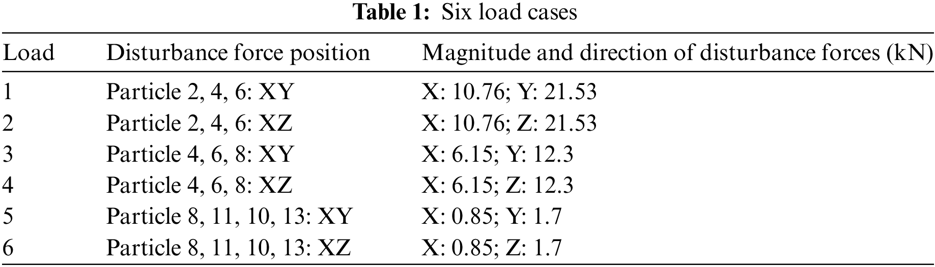
Based on the relevant equipment parameters, the first step is to determine the high-frequency disturbance force generated by the upper high-frequency unit. Quantitative analysis of the disturbance is achieved by manually calculating the force using the relevant weight and speed parameters. According to the ‘Design Standard for Dynamic Machine Foundations’ (GB50040-2020), the formula for calculating machine disturbance force can be obtained, which determines that the size of the disturbance force is only related to the weight of the equipment rotor and its speed. Since the upper unit consists of three different parts, resulting in different disturbance force magnitudes at different locations of the top plate. The calculation formulas of lateral and vertical disturbance force and longitudinal force are shown below:
Based on the calculated disturbance forces, six load cases combinations are formed in Table 1 to represent the high-frequency disturbance inputs of the unit. Each disturbance condition acts on the corresponding location.
When designing a machine foundation, the time-history function of the input disturbance is usually assumed to be a sinusoidal wave under stable operating conditions. However, in the case of considering the moment when the disturbance is applied to the foundation structure in finite element analysis software, it is simulated as a ‘sudden load’ input. Based on the knowledge of structural dynamics, when a structure is subjected to a ‘sudden load’, the generated dynamic response is generally considered to be about twice as large as the original results. However, this assumption is not consistent with the actual situation.
2.5 The Finite Element Computational Model
In this example, the entity units of the finite element calculation model are built according to the above results and the given parameters. ABAQUS 6.14-2 is used for modeling and calculation, and the relevant modeling methods are as follows:
(1) First, add the top plate and column groups in the “Part” process, and model according to the size of the structure, completing the opening at the corresponding position of the top plate. The dimensions of the top plate are 8800 mm × 3500 mm × 1200 mm, the middle column is 800 mm × 800 mm, and the edge column is 1000 mm × 1000 mm.
(2) In the “Property” column, material properties are created based on the on-site test report, specifying its mass density and relevant elastic parameters. Since the dynamic process analysis is within the scope of small elastic deformation, only the elastic modulus and Poisson’s ratio of the elastic phase need to be considered. According to the concrete-related parameters, the elastic modulus is 24786.34 N/mm2, and the Poisson’s ratio is 0.193.
(3) In the “Assembly” column, select the creation of instances, and complete the assembly of the four edge columns and four middle columns with the top plate. Complete the assembly step according to the arrangement of the structure.
(4) In the “Loads” column, first create the self-weight item of the equipment, and apply the actual calculated upper equipment self-weight on the top plate, including the load of three parts of the unit. At the same time, create the disturbance force time history function, and apply the obtained disturbance force amplitude and input frequency in the form of a sine function at the specified position of the top plate to form dynamic disturbance force input. Also, complete the fixed connection at the column base, considered as the lower end fixed, with no rotational and displacement in X, Y, and Z directions.
(5) In the “Analysis Step” column, create two analysis steps, including the initial process of the first part, applying the unit self-weight repositioning on the top plate, and complete the application of the structure’s weight. This is the static analysis step. Next, create the disturbance force time history analysis, create dynamic implicit, and set the maximum number of steps and the size of the initial increment step to limit the number of dynamic calculations and the number of steps in the calculation.
(6) In the “Mesh” column, the structure is divided into meshes, and the structure needs to be divided and manually swept to form hexahedral elements. The principle of its subdivision is to avoid irregular and concentrated element situations as much as possible. A good element mesh is conducive to the efficiency of later dynamic calculations. Mash division refers to Fig. 1.
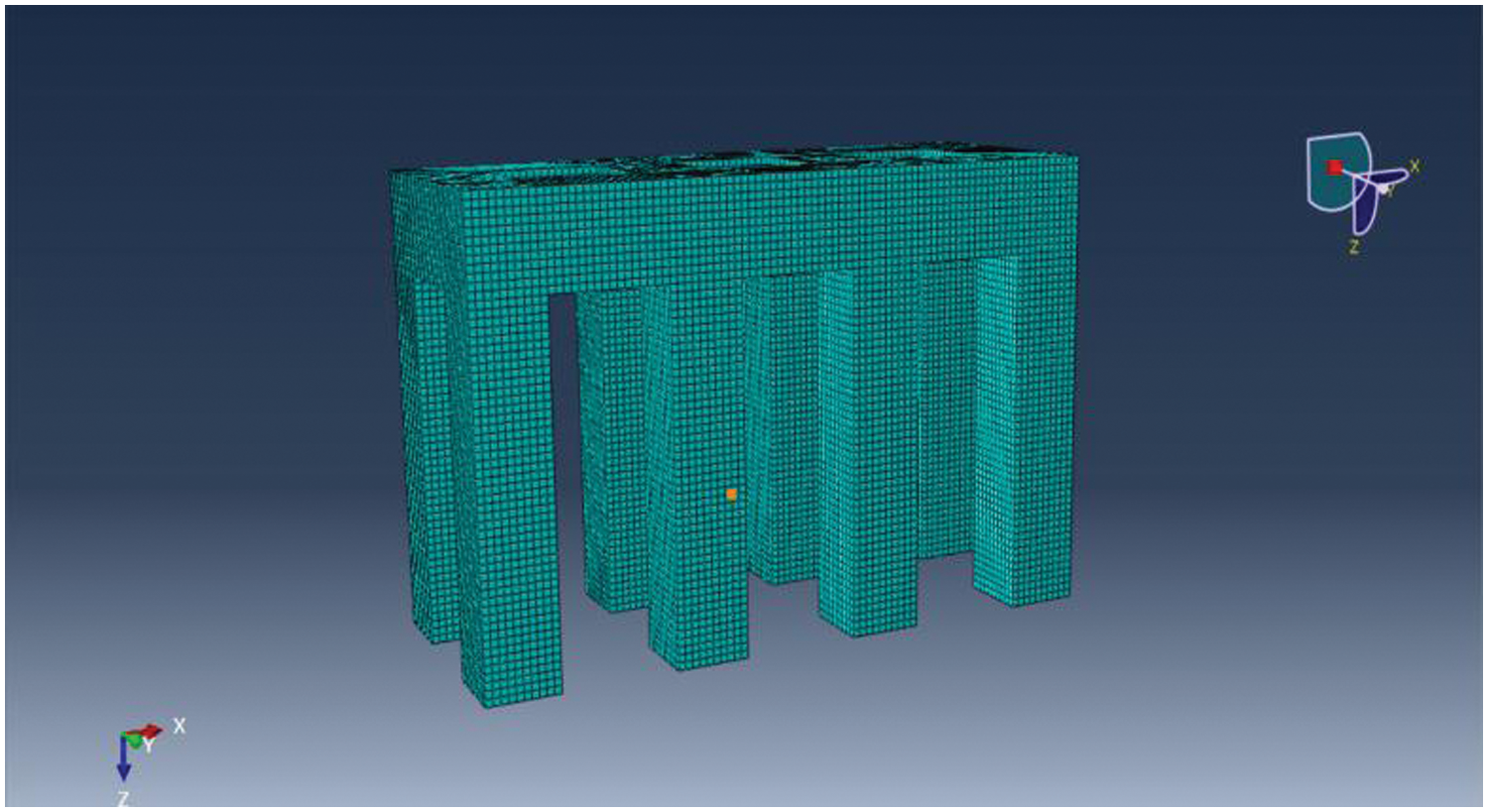
Figure 1: The finite element computational model
(7) In the “Job” column, create a task and perform a data check, ensure that the task is error-free, and then submit it to obtain the result of the dynamic analysis.
(8) After the ABAQUS calculation is completed, the corresponding output database file will be obtained, which can be opened through the software and visualized to check the simulated results. The result can be obtained through stress and displacement contour plots of the top plate and data output. The result data can be output to Excel or plotted in graph form.
The natural frequency of the system is 110.62 rad/s, with a natural period of 0.057 s. In comparison to the traditional simplified rod system, the overall stiffness is lower. Through research, it has been found that when the simplified rod system calculation model explores up to the 33rd order of modes, the error will correspondingly increase exponentially. Moreover, when studying the dynamic response of the foundation under high-frequency vibration disturbance exceeding 5400 rpm, the use of solid element model analysis provides more accurate results.
2.6 Analysis of Fundamental Dynamic Response Results
Based on the previous simulation results and conventional design, the startup process of the unit is not considered especially under high speed and high frequency. During the startup process, the frequency of the unit will pass through the foundation’s natural frequency region, causing a sudden increase in amplitude. Therefore, it is necessary to analyze the dynamic response of the foundation during this process. In general, the amplitude generated by the ‘sudden load’ in dynamic foundation design analysis is usually larger than the amplitude generated under stable operating conditions, resulting in the loss of important analysis results. The dynamic analysis results at a certain point are shown in Fig. 2.
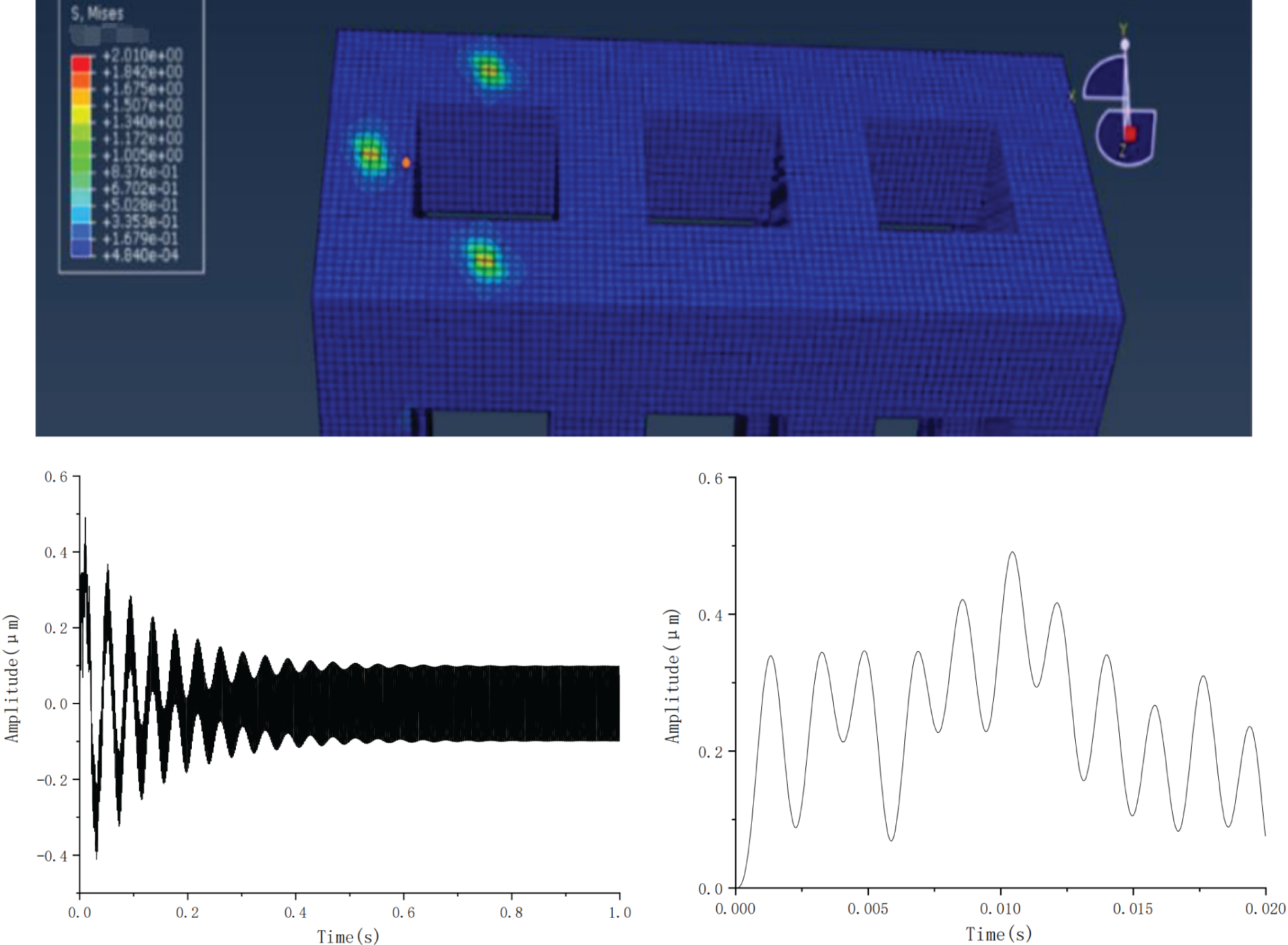
Figure 2: Dynamic response of the structure under disturbance and sudden load in the first 0.02 s
Based on the dynamic response results shown in the figure above, when the high-frequency disturbance of the turbine unit is input under stable operating conditions (including fixed disturbance input circular frequency and disturbance amplitude), the generated dynamic response and amplitude should fluctuate around the horizontal line of zero amplitude. However, it is important to note that the results of the dynamic response within the short time range (0.02 s) before the disturbance input differ from the overall process, as shown in Fig. 2. The amplitude generated during this process fluctuates around 0.2 micrometers and reaches a maximum value of 0.5 micrometers after 0.01 s. This maximum amplitude value includes the steady process. Therefore, to obtain the accurate dynamic response results of the foundation under high-frequency disturbance, it is necessary to simulate the startup condition and conduct a comprehensive analysis of the foundation’s dynamic response throughout the whole process.
Due to the increasing frequency and amplitude of disturbance during the startup process of high-frequency units, it will inevitably pass through the natural frequency region of the lower foundation at a certain point, resulting in the so-called ‘resonance’. When a structure undergoes resonance, its dynamic response suddenly increases, highlighting the importance of considering the magnitude of the structural dynamic response during this process. Currently, there is no specific and clear research in the field of dynamic foundation design on the startup problem, which is indeed significant in structural vibration.
In this study, we propose a time-history function for simulating the startup condition of a high-frequency unit by considering relevant parameters and apply this function to analyze the dynamic response of the foundation during the startup process. This research aims to fill the gap in understanding the influence of the startup condition on the dynamic response of machine foundations.
3 High-Frequency Unit Start Disturbance Force Model
3.1 High-Frequency Unit Startup Methods
There are various methods for starting units, and the difference of types and its functional application may influence the starting method and its effects. The unit starting methods can be categorized as follow Table 2.
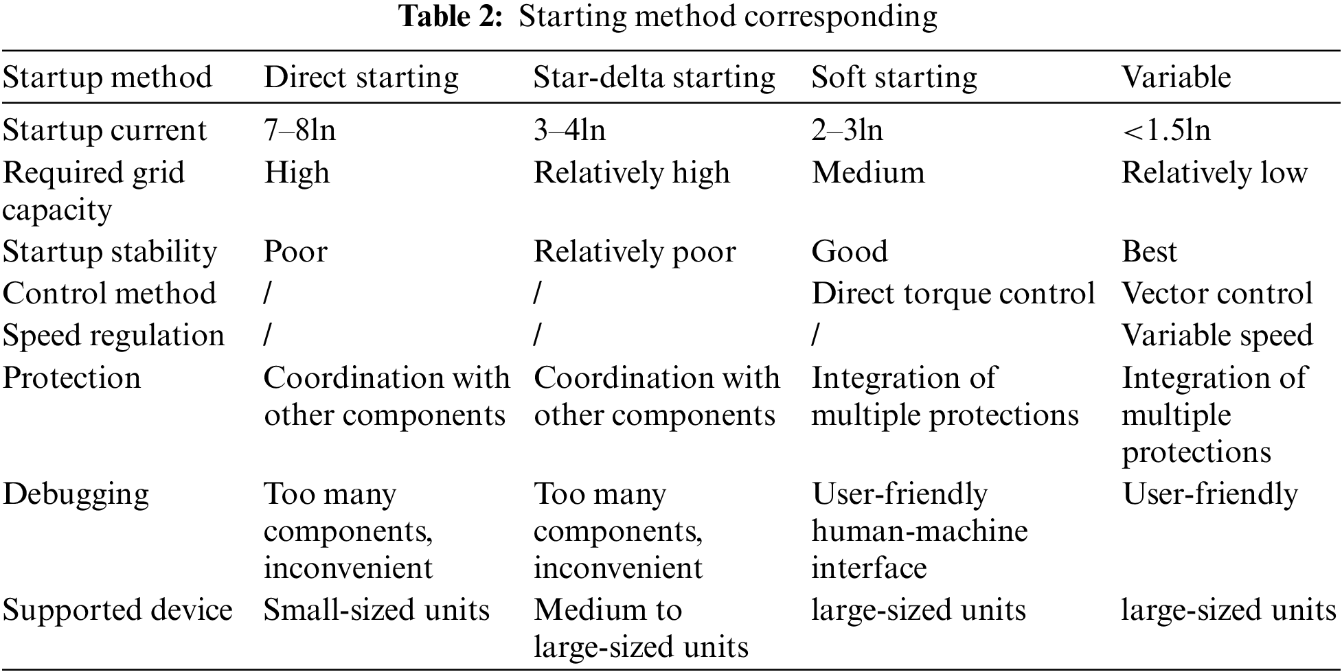
This study proposes a time-history function for frequency and disturbance amplitude, coupled with the final machine startup time-history function, based on the compressor startup time provided by the equipment manufacturer.
Table 3 shows the relevant technical parameters for the unit startup provided by the manufacturer. Based on Table 3, the high-frequency unit in this study takes a total time of 1.016 s from startup to steady operation.
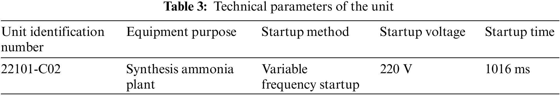
3.2 Startup Frequency-Time Function of High-Frequency Unit
The startup method of the high-frequency unit is variable frequency starting, with the main starting device modules comprising control drive circuitry and the main circuit. The advantage of choosing variable frequency starting for this large-scale unit lies in its ability to effectively control variations in current and voltage within the dynamic grid, enabling efficient frequency transformation and simultaneous protection of the circuitry and dynamic grid. In accordance with the principles of motor operation, the variable frequency starting method enables flexible startup and precise speed control of the motor, thereby achieving optimal startup performance. Additionally, this startup method offers benefits such as energy efficiency, stability, and reliability, making it suitable for meeting the design requirements of high-frequency, high-dynamic units. Furthermore, it significantly reduces operational costs and enhances equipment efficiency:
Obviously, to control frequency changes and stable voltage, it is necessary to change the magnetic flux. By relying on the nonlinear characteristics of the iron core of the variable frequency motor, the magnetization size can be changed. However, it should be noted that it cannot exceed the range of being too large or too small. Another method is to control the voltage change to achieve frequency conversion while maintaining as a fixed value to ensure
Based on the original startup time provided by the mechanical manufacturer, a high-frequency unit simulation startup frequency function can be proposed:
Specifically,
3.3 Startup Disturbance Amplitude-Time Function of High-Frequency Unit
The disturbance force generated by the unit is related to the weight of the unit’s rotor and its rotational speed. During startup, the weight of the rotor remains constant, but its rotational speed varies with the working frequency and is positively correlated with the unit’s speed, resulting in a time-dependent change in machine speed during the startup process. Based on the relationship between speed and disturbance force amplitude provided by the specifications, it is determined that the disturbance force amplitude is proportional to the 3/2 power of the speed. Since the speed is linearly related to the startup time, the disturbance force amplitude follows a 3/2 power law with respect to time. By combining the simulated startup frequency function and relevant machine design parameters provided by the manufacturer, a linear function for simulating startup disturbance force amplitude is proposed:
To illustrate with an example, the disturbance amplitude vs. time profile during the startup process is represented by selecting the most unfavorable steady-state working disturbance amplitude. This is achieved by choosing
3.4 Coupled Generation of Simulated Startup Perturbation Models for High-Frequency Units
The startup process of high-frequency units should consider the variations in frequency and disturbance force amplitude. At each moment during startup, there is an instantaneous frequency and disturbance force amplitude. This requires coupling the previously provided functions for frequency and disturbance force amplitude variations over time to generate a simulated machine startup condition function. Referring to the general working principles of variable frequency machines, the disturbance force-time function is assumed to be sinusoidal in shape. As a result, the coupling result of the simulated startup condition function is proposed as follows:
In this example, the maximum force amplitude k is equal to 21.56 kN, the steady-state circular frequency is 1105.24 rad/s, and the total startup duration is 1.016 s. The simulated startup conditions are illustrated in Fig. 3, depicting partial startup function curves.
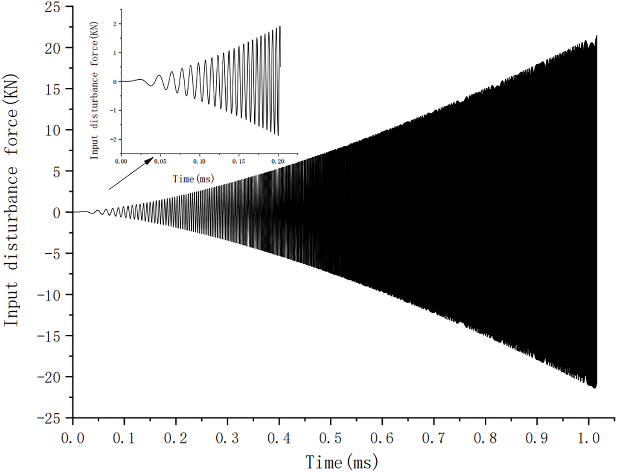
Figure 3: Input disturbance function under simulated starting condition
4 Analysis of Foundation Dynamic Response under Simulated Startup Conditions of High-Frequency Units
In analyzing the dynamic response of the foundation under simulated startup conditions of high-frequency units, it is crucial to pay attention to the amplitude of the foundation slab when the startup disturbance circle frequency is close to the fundamental frequency. By utilizing the relevant parameters of an example model, the fundamental dynamic response of a high-frequency unit under simulated startup conditions is examined. Specifically, the focus is on investigating the amplitude variations at the most critical node of the structure’s top plate as the frequency and amplitude of the input disturbance condition function change with time. This simulation process is built upon the analysis conducted in Chapters 2 and 3, with the main difference being the replacement of the steady-state disturbance input time function with the disturbance time function for simulating the startup process. Instead of a sudden disturbance, the simulated startup condition function gradually increases from zero to a stable operating condition. Additionally, the time step for dynamic analysis in the software needs to be considered. The following discussion will delve into the influence of the dynamic analysis time step on the overall dynamic response results, determine the optimal step size, and complete the analysis of the dynamic response effectively.
4.1 Transient Dynamics Analysis Step Selection during Startup
Analyzing the startup conditions of high-frequency units necessarily involves transient dynamics in variable frequency systems. In this aspect of the analysis, the measurement of the calculation analysis step size has been extensively studied by many scholars due to its crucial importance in determining the accuracy and rationality of the results. A suitable choice of the time step will determine the validity of the overall finite element calculation and could even result in ignoring the maximum data point problem in the analysis process due to sparse time-step values, especially in the analysis of higher-order modal. For this reason, it is vital to correctly choose the calculation and analysis step size for analyzing the dynamic response of high-frequency disturbance. A step size that is too short would result in a significant amount of computation time and resources wasted on obtaining essentially identical results.
To select the appropriate time step for analyzing the fundamental dynamic response of the foundation under high-frequency units, the following principles should be followed:
(1) Analyze the frequency of the response: The reasonable integration time step should capture the dynamic response results adequately within each cycle, forming a combination of modal forms. Effective higher-order modal can serve as a reference for the required solution in the time step. In the case of the NEWMARK integration scheme, a suitable integration time step can take n between 20 to 40 points per cycle as a reference to determine the optimal step size.
When calculating the acceleration in further computing of dynamic response, it is obvious that a larger value of n is required. According to the research of some scholars, n can be set to 60, which will reduce the integration time step.
(2) Analyze the load-time curve: When considering the calculation time step, it is inevitable to consider its relationship with the dynamic loading frequency. The chosen time step should be smaller than the minimum period of the dynamic loading. The dynamic response of the structure is often slower than the input loading, and selecting a shorter calculation time step will help to comprehensively capture changes in the loading dynamics.
(3) Analyze the wave propagation: When waves propagate, their impact on the analysis should be carefully considered. The time step should be small enough to capture the information between adjacent wave peaks or troughs.
(4) Meet the accuracy criteria for the time step: The finite element calculation cycle is based on the specified time step, and the dynamic equilibrium equation is solved on these discrete time points while following the laws of dynamics within each time step. The dynamic response within a time step that is smaller than the minimum period can be represented by the results of adjacent discrete points whose contour is enveloped by reasonable time step results. In cases where a larger time step is selected, the continuous response results within the time step would not comply with the laws of dynamics, leading to erroneous conclusions. In appropriate conditions, MIDTOL can be introduced to halve and correct the corresponding results, solving these special problems using a mean-value approach.
Based on the principles for selecting the time step, considering the calculation duration and accuracy, the time step is determined as
4.2 Dynamic Response Analysis under Simulated Startup Process
Based on the background of the high-frequency compression unit in this project, the model is constructed to analyze the fundamental dynamic response considering the startup conditions of the high-frequency unit, where the input disturbance is the startup load-time function. In this analysis, the focus is on the impact of variations in frequency and disturbance amplitude under the startup conditions of the unit on the structural dynamic response. Therefore, the most unfavorable conditions are selected as the analytical premise for various control factors, such as the stable operating circular frequency of the high-frequency unit, load combinations, and node analysis. The following parameters are chosen: the most unfavorable operating circular frequency
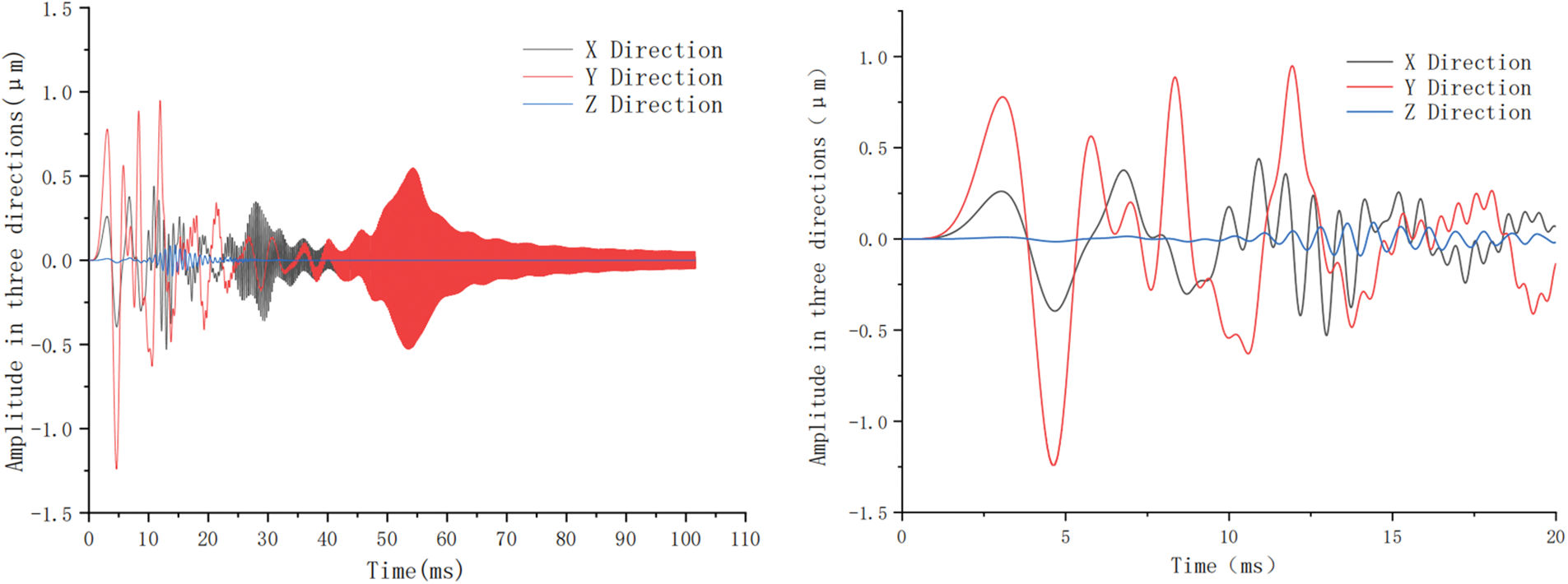
Figure 4: Dynamic response under simulated starting condition
The maximum amplitude at node 2 occurs 4.7 milliseconds after startup, with a maximum amplitude of 1.22 micrometers in the Y direction. Analysis of the overall response curve reveals two regions of amplitude mutation: the first is the area near the fundamental frequency of the input disturbance, and the second is the region where the fundamental vibration mode is concentrated, which exhibits sudden amplitude increases. These two regions occur during the 0–20 millisecond and 40–60 millisecond stages after startup. The amplitude response reaches a stable stage approximately 95 milliseconds after startup.
Regarding the analysis of the fundamental frequency crossing, it was found that the amplitude curve exhibits significant fluctuations at the beginning of startup, and the maximum amplitude occurs near the structural fundamental frequency. The amplitude then gradually decreases as it stabilizes, reaching approximately one-tenth of the maximum value. Fig. 4 shows the top plate amplitude response of the high-frequency unit during the first 20 milliseconds of startup. Refer to Fig. 4 for the dynamic response structure of the foundation structure.
Analysis of the Y-directional amplitude reveals that the second amplitude wave occurs in the structural vibration mode intensity during the 40–60 millisecond stage. However, the response size is completely enveloped by the maximum amplitude of the first wave. The amplitude stabilizes approximately 95 milliseconds after startup, with a stable amplitude of approximately 0.05 micrometers, which is much smaller than the amplitude in the wave region. This can be considered as the fundamental structural dynamic response at the stable working frequency, which is essentially reached at the final stage of the startup process, approximately the last 20 milliseconds before the amplitude stabilizes. This is illustrated in Fig. 5.
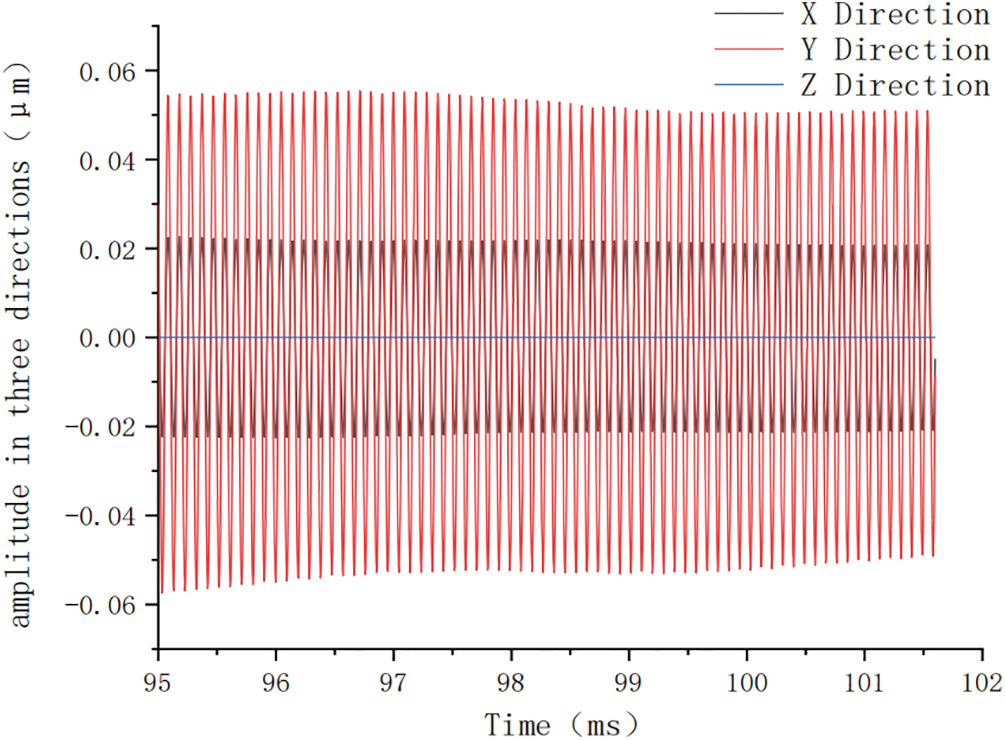
Figure 5: Dynamic response curve at the end of startup
5 Considering the Results of the Dynamic Foundation Response for Different startup Durations
In general, the total startup time of high-frequency units varies, resulting in different degrees of resonance during the startup process as they cross the lower fundamental frequency. Prolonged operation within the fundamental frequency zone can cause sudden increases in the amplitude of the top plate, with significant increases in magnitude. Therefore, it is necessary to further analyze the corresponding dynamic responses and the impact on the lower foundation to effectively control the allowable total startup time of the unit. The startup duration must be appropriately extended and dynamic analysis must be performed.
Considering the rated startup time of the unit at 1016 milliseconds, it is necessary to analyze the results and propose relevant design suggestions based on the extension of the startup time by equal multiples. startup times of 2032 milliseconds, 3048 milliseconds, and longer durations were evaluated, and the regular patterns based on the total startup time were summarized.
5.2 Proposal of Startup Load History Functions
To utilize the startup properties of the unit, corresponding schedule functions for startup frequency and startup disturbance force amplitude were proposed, and a simulated startup operating condition function was generated for this specific total startup time, similar to the 1016-microsecond work situation proposed earlier. The coupling of the simulated startup operating condition function was completed with reference to the following equation:
y simply changing the total startup time in Eq. (13), different startup durations can be generated. Taking a total startup time of 2032 milliseconds and 3048 milliseconds as examples, the simulated startup operating condition function of the unit was coupled and generated.
In this study, the simulated startup operating condition function of the unit was generated under the worst-case scenario. The maximum disturbance force amplitude Fs was set to 21.56 kN, and the stable working circular frequency
The related simulated startup function image is shown in Fig. 6 below.
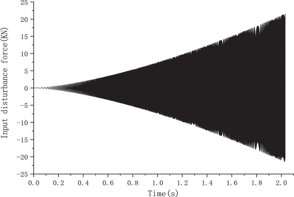
Figure 6: Simulation startup time history function when the total startup time is 2032 microseconds
Furthermore, with a total startup time of 3048 microseconds, the expression of the result after coupling the startup schedule function of the high-frequency unit is as follows:
By utilizing this simulated startup function, various startup operating conditions can be defined based on different total startup times. Due to space limitations, only these two typical startup times have been analyzed. The simulated startup operating condition function was then input into the finite element model of the foundation structure for transient dynamic analysis.
Referring to the structural analysis method described in the previous section, the two schedule functions with startup times of 2032 microseconds and 3048 microseconds were input into the foundation structure of the high-frequency unit for dynamic response analysis during the startup process. The foundation dynamic results for the different startup durations are shown in Fig. 7.
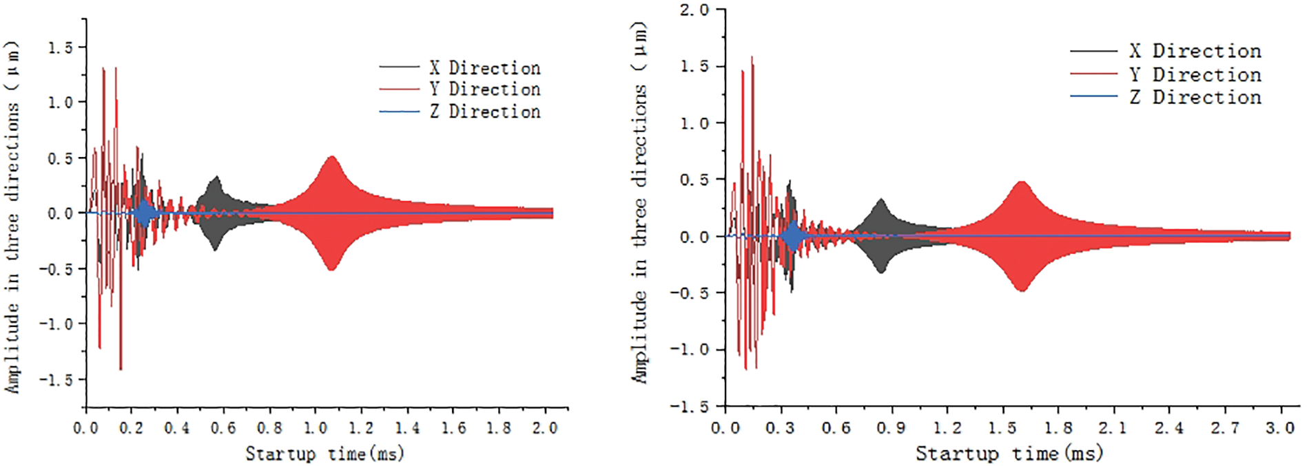
Figure 7: Simulated startup time history function when startup time are 2032 and 3048 microseconds
Based on the analysis of the dynamic response results of the foundation structure under high-frequency excitations, it can be observed that when the total startup time of the unit is set to 1016 milliseconds (T), the maximum amplitude of the top plate during the passage through the lower foundation’s fundamental frequency region is 1.25 micrometers. When the startup time is extended to 2032 milliseconds (2T), the maximum amplitude of the top plate throughout the entire process increases to 1.48 micrometers. Similarly, when the startup time is further extended to 3048 milliseconds (3T), the maximum amplitude of the top plate during the entire process further increases to 1.63 micrometers. Therefore, it can be preliminarily concluded that as the total startup time of the upper unit increases, the maximum amplitude of the foundation’s top plate during the startup process also increases.
Furthermore, this study seeks to determine the maximum permissible startup time that allows for a controlled amplitude of approximately 4 micrometers for this engineering case. It is found that when the startup time is set to 7112 milliseconds (7T), the maximum amplitude of the top plate still meets the permissible requirements. However, when the startup time is extended to 8128 milliseconds (8T), the maximum amplitude of the top plate exceeds the allowable limit, failing to meet the required specifications in the design code. Therefore, it is necessary to consider the influence of changes in the total startup time of the upper unit on the dynamic response of the lower foundation structure during the structural design process.
6 Conclusions and Design Recommendations
6.1 Sorting out the Conclusions of the Dynamic Response of the Startup Process
This paper presents frequency and excitation amplitude time functions during the startup process of high-frequency units and integrates them to generate a simulated startup time function for a high-frequency unit, which is then input into the structural analysis to determine the dynamic response while crossing the foundation frequency region. The finite element numerical calculation results exhibit a slight discrepancy compared to the on-site monitoring results, with an error of approximately 6%. The primary focus is on the magnitude of the dynamic response when the excitation frequency is close to the foundation frequency. Utilizing transient dynamic content of variable frequency, the instantaneous dynamic analysis step size during the startup process is computed to accurately meet the highest-order mode calculation requirements. The study further investigates the dynamic response of the foundation under different startup durations by simulating the dynamic response under two startup durations of 2032 microseconds and 3048 microseconds. It is concluded that the longer the total startup time, the smaller the stable line displacement amplitude generated during startup.
(1) The fluctuations in the amplitude of the top plate during the startup process of high-frequency units generally occur at two locations. The first location is near the structural fundamental frequency region that the unit passes through, while the second location is the region with a relatively dense distribution of vibration modes before the top plate’s amplitude reaches stability (the 2/5 to 3/5 portion of the startup time). Generally, the maximum top plate amplitude occurring in the denser mode distribution area can be enveloped by the maximum value of the first stage amplitude fluctuations, which is assumed to occur near the foundation frequency of the unit during high-frequency unit startup.
(2) In comparison to the general design of high-frequency dynamic foundations, which analyzes the dynamic response by inputting stable operating excitation functions during simulation, the maximum amplitude obtained considering the unit’s startup condition is less than that obtained when a similar sudden load is applied to the structure. The maximum amplitude obtained under the startup condition aligns closer to the actual situation than directly inputting stable operating excitation functions, which enhances its persuasiveness. This offers relatively extensive optimization space for future design improvements.
(3) As the startup time increases, the maximum displacement generated also increases when the rated operational frequency and excitation amplitude are the same. The position where the maximum displacement occurs is near the frequency at which the machine input simulation excitation frequency equals the structural natural frequency.
(4) During the startup process to reach the stable startup region within the specified startup time, the change in the line displacement amplitude is minimal. The longer the total startup time, the smaller the stable line displacement amplitude generated during startup. As shown in Fig. 8.
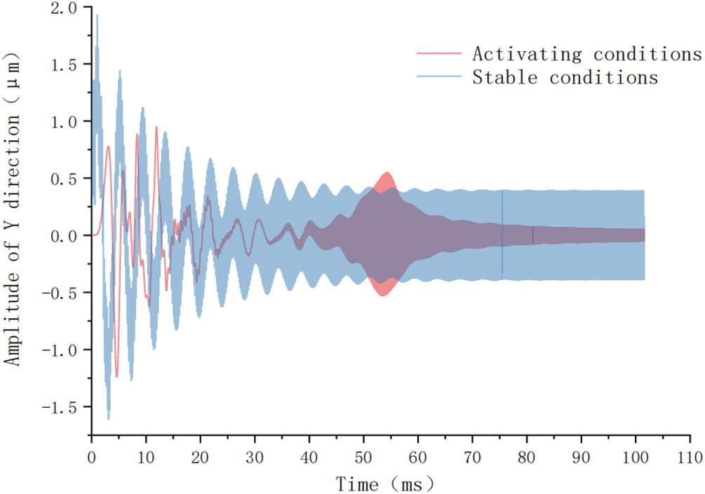
Figure 8: Input comparison of different disturbance modes
(5) It is crucial to consider the impact of the total startup time on the dynamic response of the lower structure during the unit’s startup process. Excessively long startup time may lead to excessive resonance when the excitation frequency crosses the foundation frequency, resulting in excessive top plate amplitude.
6.2 Design Recommendations Considering High-Frequency Unit Startup Conditions
(1) In the initial phase of activating high-frequency units, it is inevitable to pass through the natural frequency range of the lower structure, leading to resonances with sudden increases in displacement of the top plate. The maximum amplitude of the top plate, being the predominant controlling factor, reaches the peak value during the entire dynamic analysis process, emphasizing the need to consider the impact of the startup process.
(2) Analysis of the most critical time points during the startup process primarily focuses on the location where the input excitation frequency aligns with the foundation’s natural frequency and the area with concentrated vibration modes.
(3) During startup simulation, the resonant region (maximum line displacement) can be quickly identified, and the maximum line displacement amplitude can be approximately estimated without completing the entire dynamic analysis process.
(4) It can be approximated that the dynamic response stabilizes under steady working conditions after 4/5 of the total startup time.
(5) Considering the startup condition, the duration of the startup process is a crucial factor that cannot be overlooked. The recommended maximum duration for unit startup should be included in the design conclusion to prevent excessive adverse vibrations of the lower foundation and excessive top plate amplitude.
Acknowledgement: I would like to express my gratitude for the assistance and guidance provided by Professor Gao Jianling and Professor Bai Yuxing from North China University of Technology in the research of this project.
Funding Statement: Smart Integration Key Technologies and Application Demonstrations of Large Scale Underground Space Disaster Prevention and Reduction in Guangzhou International Financial City ([2021]–KJ058). URL: http://www.gzmcg.com/.
Author Contributions: Study conception and design: Mingwei Hu, Dawei Ruan; data collection: Dawei Ruan; analysis and interpretation of results: Dawei Ruan, Mingwei Hu; draft manuscript preparation: Dawei Ruan. All authors reviewed the results and approved the final version of the manuscript.
Availability of Data and Materials: The data that support the findings of this study are available on request from the first author upon reasonable request.
Conflicts of Interest: The authors declare that they have no conflicts of interest to report regarding the present study.
References
1. Jeong, G., Jung, M., Park, S., Park, M., Ahn, C. (2024). Contextual multimodal approach for recognizing concurrent activities of equipment in tunnel construction projects. Automation in Construction, 158, 105195. [Google Scholar]
2. Zhong, T., Feng, X., Zhang, Y., Zhou, J. (2020). Multiple-TMD-based structural vibration control for pumped storage power plants. Applied Sciences, 10(16), 5577. [Google Scholar]
3. Xu, J., Shi, H., Sun, F., Tang, Z., Li, S. et al. (2022). High-frequency vibration analysis of piezoelectric array sensor under lateral-field-excitation based on crystals with 3 m point group. Sensors, 22(9), 3596 [Google Scholar] [PubMed]
4. Verma, M., Lafarga, V., Dehaeze, T., Collette, C. (2020). Multi-degree of freedom isolation system with high frequency roll-off for drone camera stabilization. IEEE Access, 8, 176188–176201. [Google Scholar]
5. Xia, H. S., Liu, X. T., Zhang, C. (2018). A study on contemporary urban rail transportation hub theory and the development trend. World Architecture, 2018(4), 10–15+117 (In Chinese). [Google Scholar]
6. Zhang, L., Lei, X. Y., Feng, Q. S. (2019). Testing analysis of structural vibration propagation in high-speed rail comprehensive transportation hub station. SCIENTIA SINICA Technologica, 49(9), 1107–1116. [Google Scholar]
7. Pei, Y. X., Zhang, K. F., Dai, K. D. (2003). Dynamic analysis and design of block type foundation for reciprocating compressor. Building Structure, 11, 36–38 (In Chinese). [Google Scholar]
8. He, H. B., Sheng, Z. P., Zhou, S. Z. (2004). Analysis on vibration of block foundation of natural gas compressor. China Petroleum Machinery, 32(9), 7–8 (In Chinese). [Google Scholar]
9. Wang, X. K., Li, Y. L. (2014). On simplified formula of vibration for foundation under reciprocating engines. Industrial Construction, 44(8), 118–120 (In Chinese). [Google Scholar]
10. Reissner, E. S. (1936). Stationäre, axialsymmetrische, durch eine schüttelnde Masse erregte Schwingungen eines homogenen elastischen Halbraumes. Archive of Applied Mechanics, 7(6), 381–396. [Google Scholar]
11. Barkan, D. D., Drashevska, L. (1960). Dynamics of bases and foundations. America: McGraw-Hill. [Google Scholar]
12. Hwang, S. W., Jeong, W. B., Yoo, W. S., Kim, K. H. (2004). Transmission path analysis of noise and vibration in a rotary compressor by statistical energy analysis. Journal of Mechanical Science and Technology, 18(11), 1909–1915. [Google Scholar]
13. Robertson, I. A. (1966). Forced vertical vibration of a rigid circular disc on a semi-infinite solid. Mathematical Proceedings of the Cambridge Philosophical Society, 62(3), 547–553. [Google Scholar]
14. Wang, J. X. (1982). Simplified method for dynamic calculation of solid machine foundation. Industrial Construction, 12(8), 38–45 (In Chinese). [Google Scholar]
15. Mihaly, M. (1977). Machine support design based on vibration calculus. UK: Collet’s LTD. [Google Scholar]
16. Zhu, Y. B. (2019). Structure design and characteristic research for 7MW offshore wind turbine pile foundation (In Chinese). China: Harbin Engineering University. [Google Scholar]
17. Luo, Z., Han, Q. K., Wang, D. Y., Luo, Y. Q. (2013). Fundamental theory for similar design of the dynamic behavior of structural components in large-scale high-speed rotating machinery foundation units. Digital Manufacture Science, 2, 1–70 (In Chinese). [Google Scholar]
18. Zhang, Z., Zhang, Z. P., Li, H. B., Qin, C. H., Guo, J. et al. (2016). A reduced method of estimating structural dynamics response under basic excitation. Structure & Environment Engineering, 43(5), 1–6 (In Chinese). [Google Scholar]
19. Xu, G., Zhao, F., Liu, T. (2023). I-f closed-loop starting strategy of high-speed PMSM based on current vector adaptive regulation. IET Power Electronics, 16, 2724–2738. [Google Scholar]
20. Ruan, D. W., Ji, X. (2021). Review of design methods for dynamic machine foundations. China Science and Technology Information, 2021(17), 58–61 (In Chinese). [Google Scholar]
21. Niu, Z. W., Wang, R. C., Zheng, R. F. (2018). Analysis on the dynamic response of shaking table foundation. Building Structure, 48(S2), 896–901 (In Chinese). [Google Scholar]
Cite This Article
 Copyright © 2024 The Author(s). Published by Tech Science Press.
This work is licensed under a Creative Commons Attribution 4.0 International License , which permits unrestricted use, distribution, and reproduction in any medium, provided the original work is properly cited.
 Downloads
 Citation Tools