Finite Element Simulations of the Localized Failure and Fracture Propagation in Cohesive Materials with Friction

1  Introduction

Microcrack/microvoid evolution and irreversible deformations, characterized by strain localization, are prevalent in solid materials such as composites, geotechnical materials, and metals. These localized behaviors are widely recognized as fundamental mechanisms leading to progressive failures and catastrophic structural collapse. Strain localization in solids leads to a softening regime in the stress-strain curve, displaying macroscopic strain/displacement discontinuities. These characteristics inherently limit the applicability of continuum-based approaches, including material models. Despite significant advancements in understanding localized failure through pioneering studies, achieving high-fidelity modeling of this behavior remains a challenging issue in engineering.

Within the geotechnical sphere, slope failure, known as landslides, represents a common geotechnical and geological hazard stemming from strain localization. Various approaches have been gradually introduced to evaluate slope stability precisely. The limit-equilibrium method (LEM) stands as one of the prominent methods, originating from early geotechnical theory and amassed engineering experience [1,2]. This method assumes slope materials undergo rigid-plastic deformation, failing to reflect strength degradation from deformation accumulation. Additionally, dynamic crack propagation due to slope instability is simplified into a static crack (i.e., the preset crack). In response to these limitations, the strength reduction method (SRM) was proposed. It assumes simultaneous strength reduction across the entire slope material zone [3,4]. However, this assumption in the SRM fails to convincingly capture the progressive formation of a slip plane [5].

Confronting the above challenge, some advanced numerical approaches have been developed in recent years to predict soil slope instabilities. These include mesh-based methods and particle-based methods. The particle-based method views a material domain as an assembly of discrete yet interactive particles or blocks. This encompasses approaches like the discrete element method (DEM) [6,7], discontinuous deformation analysis (DDA) [8], smoothed particle hydrodynamics (SPH) [9], and the material point method (MPM) [10]. These methods relieve the restrictions of meshes, thus theoretically practicable to elucidate the large deformation and discontinuity in slopes [11]. However, DEM and DDA based on particles or blocks often encounter challenges in determining particle contact parameters. Regarding SPH and MPM, Bao et al. [12] highlighted their time-consuming nature compared to FE simulations.

Consequently, the mesh-based method is currently favored in slope stability analysis. Nonetheless, the conventional finite element method (FEM) cannot directly tackle the issue of discontinuity arising from crack propagation [13]. To address this issue, advanced re-meshing techniques have been integrated into FEM, leading to the development of the extended finite element method (X-FEM) [5,14], embedded finite element method (E-FEM) [15,16], and augmented finite element (A-FEM) [17], among others. For instance, Vo et al. [18] investigated the desiccation cracking of clayey soil using FEM incorporating the damege-elastic cohesive fracture law; Wang et al. [5] explained the failure development process of soil slopes using the improved X-FEM; Barani et al. [19] and Hu et al. [20] studied the tensile cracking of cohesive soils with varying water contents by using the cohesive-model-based FE approach; de Maio et al. [21] developed a cohesive FE approach based on a modified bond-slip law to evaluate the mechanical behavior of nano‑modified FRP sheets implemented in reinforced concrete structures. These three methods introduced additional degrees of freedom (DoFs) into the cracked element, such that they account for the arbitrary intra-element discontinuities. Unlike X-FEM and E-FEM, A-FEM strictly adheres to the standard FEM process, encompassing independent element interpolation, stiffness integration, equivalent force integration, etc. Moreover, through the application of static condensation, Liu et al. [22] demonstrated the complete condensation of additional DoFs at the elemental level. Consequently, this approach maintains the advantage of not requiring additional nodes or nodal DoFs when tracking cracks within an element. Considering these factors, A-FEM has been chosen for simulating slope stability in this study.

Additionally, numerous field investigations of landslides have confirmed the crucial role of crown tensile or tensile-shear cracks in determining slope stability (see Fig. 1). However, to our knowledge, the majority of studies have primarily focused on the compression-shear failure of slopes. The impact of tension-shear cracks or an assessment considering both tension-shear and compression-shear effects on slopes remains significantly underexplored. To address this, an integrated algorithm combining a coupled cohesive zone model (CZM) considering both tension-shear and compression-shear was introduced into the A-FEM framework. Subsequently, this study conducted a comprehensive analysis of a soil slope featuring specific tensile strength to unveil failure mechanisms and scrutinize the influence of mechanical parameters in soils.

Figure 1: Survey investigations conducted on soil slopes featuring tension-shear cracks: (a) a potential landslide in the Shengzhou region of Zhejiang Province in 2023; (b) a landslide in Liaoning Province [12] (reprinted with permission from Springer Nature: Springer, Natural Hazards, “Investigation of the role of crown crack in cohesive soil slope and its effect on slope stability based on the extended finite element method,” Bao et al., © 2021); and (c) a potential landslide with tensile cracks in Jilin Province in 2015 [12] (reprinted with permission from Springer Nature: Springer, Natural Hazards, “Investigation of the role of crown crack in cohesive soil slope and its effect on slope stability based on the extended finite element method,” Bao et al., © 2021). The arrows in the images indicate the direction of movement of the sliding mass

2  Numerical Theories and Methodologies

2.1 Governing Equations with Strong Discontinuity

Consider a physical domain Ω with a boundary ∂Ω, as shown in Fig. 2. A body force per unit area b acts on Ω, and its boundary ∂Ω is decomposed into disjoint regions Γu and Γt. The prescribed displacement u¯ is imposed on Γu; the external traction t¯ is employed on Γt. Additionally, a discontinuity cuts the body into two subdomains Ω+ and Ω−, with the respective discontinuity surfaces Γc+ and Γc− (i.e., Γc = Γc+ ∪ Γc−). Suppose the constitutive law σ(u)=D:ε(u) governs the body Ω, while the cohesive zone model characterizes the discontinuity in this physical domain. Then, the differential equation for this problem can be written as:

{∇⋅σ=0(inΩ∖Γc)σ⋅n=t¯(on Γt)u=u¯(on Γu)t+=σ⋅m+=−t(on Γc+)t−=σ⋅m−=t(on Γc−)(1)

In the above equations, D represents the isotropic elasticity tensor; n denotes the outward normal vector of the stress boundary Γu; u signifies the displacement vector; t−=−t+=t are the tractions imposed on the discontinuity surface Γc; m is the outward normal vector of Γc.

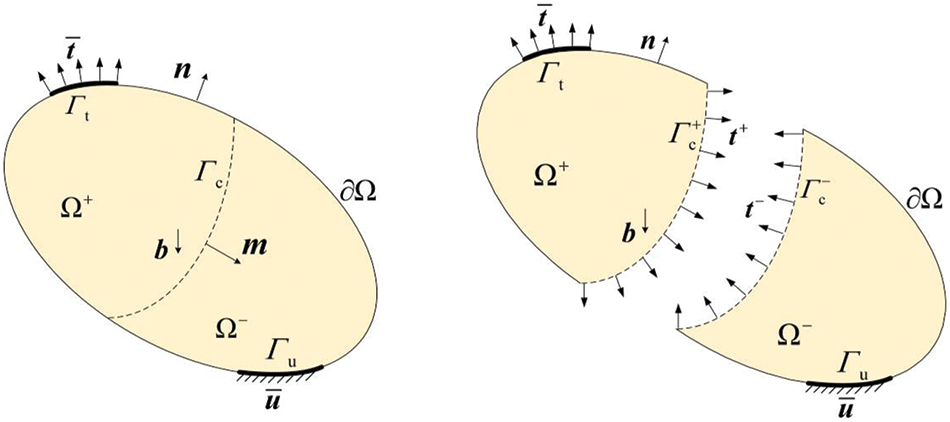
Figure 2: A 2D physical domain with discontinuity (Ω = Ω+ ∪ Ω−, ∂Ω = Γt ∪ Γu ∪ Γc)

Using the virtual work principle, the equilibrium equation Eq. (1) is further rewritten as a weak form,

∫Ω∖Γcδε:σdΩ+∫Γc+δΛu⋅tdΓ=∫Ωδu⋅bdΩ+∫Γtδu⋅t¯dΓ(2)

wherein the sign ‘δ‘ denotes a virtual value of a variable that follows, and Λu=u+−u− denotes a displacement jump vector across the material surface.

2.2 Construction of Displacement Field with N-AFEM

To ensure the numerical tool’s high fidelity and robustness, this study introduces the nonlinear A-FEM (i.e., N-AFEM). N-AFEM integrates with a constitutive model of geomaterials, specifically a tension-compression-shear coupled cohesive zone model, to simulate localized failure and fracture propagation in geotechnical structures. This section provides a concise overview of the fundamental framework of N-AFEM used to construct displacement fields involving strong discontinuities.

For simplicity, this study employs the typical four-node, quadrilateral plane element based on the N-AFEM to illustrate the scheme of the two-dimensional displacement field. Fig. 3a provides the crack propagation within the physical domain, resulting in two basic types of crack configurations in the discretized meshes: two quadrilateral sub-domains for element ‘A’ (Fig. 3b) and one triangular along with one pentagonal for element ‘B’ (Fig. 3c). At the discontinuity surface, four internal nodes (i.e., nodes 1c, 2c, 1c′, 2c′) are enriched with regular nodal DoFs (degree of freedom). A cohesive element based on nodes 1c, 2c, 1c′, 2c′ links the two subdomains. Consequently, the cracked element is now augmented into three transitional sub-elements: two regular sub-elements for the solid domain and one cohesive element for the discontinuous crack. The incremental equilibrium equation for both cracked configurations can be unified using Eq. (2).

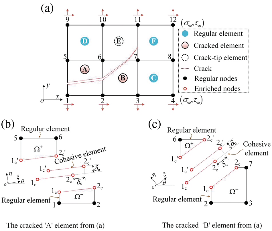
Figure 3: Schematic diagram of arbitrary intraelement cracking for N-AFEM

For the regular element Ω+,

[K11+K12+K21+K22+]{Δuext+Δuint+}={Δfext+Δfint+}(3a)

For the regular element Ω−,

[K11−K12−K21−K22−]{Δuext−Δuint−}={Δfext−Δfint−}(3b)

For the cohesive element,

[K11cohK12cohK21cohK22coh]{Δuint−Δuint+}={Δfint−cohΔfint+coh}(3c)

where Kij± denotes the tangent matrix for regular elements, displaying forms entirely identical to those found in conventional FEM; Kijcoh denotes the tangent matrix of the cohesive element, with its components contingent upon the form of the CZM outlined in Section 2.3; Δuext± and Δuint± refer to incremental displacements of external and internal nodes. Additionally, Δfωe (where ω = ext and int) signifies the incremental nodal force regarding regular and cohesive elements.

A condensation scheme that fully condenses the additional DoFs at the elemental level is employed for the N-AFEM. The condensation procedures of the N-AFEM, as per Eqs. (3a)–(3c), are outlined herein. Initially, achieving elemental equilibrium along the shared edges of 1c2c and 1c′2c′ for both the regular and cohesive elements is necessary, denoted by:

Δfint++Δfint+coh≅0Δfint−+Δfint−coh≅0(4)

Next, we substitute Eqs. (3a)–(3c), into Eq. (4), enabling the expression of the internal nodal displacements in terms of the external nodes, denoted as:

{Δuint−=(Φ1)−1K12coh(Φ2)−1K21+Δuext+−(Φ1)−1Φ3Δuext−Δuint+=(Φ2)−1K21coh(Φ1)−1K21−Δuext−−(Φ2)−1K21+Δuext+(5)

where Φ1=K22−+K11coh, Φ2=K22++K22coh−K21coh(Φ1)−1K12coh, Φ3=K12coh(Φ2)−1K21coh(Φ1)−1K21−+K21−.

Substituting Eq. (5) back into Eqs. (3a) and (3b), and subsequently eliminating Δfint+, Δfint−, Δfint−coh and Δfint+coh, we can obtain the condensed incremental equilibrium equation devoid of internal nodal forces or displacements,

[K11−−K12−(Φ1)−1Φ3K12−(Φ1)−1K12coh(Φ2)−1K21+K12+(Φ2)−1K21coh(Φ1)−1K21−K11+−K12+(Φ2)−1K21+]{Δuext−Δuext+}={Δfext−Δfext+}(6)

2.3 Post-Localization Constitutive Model

In this section, a user-defined cohesive element is introduced to characterize the intense deformation of previously formed discontinuous surfaces, accounting for the coupling between cohesive and frictional behaviors in geomaterials. Considering the uniformity of the cohesive element’s format and implementation procedures [23], this section primarily focuses on elucidating the inherent structure of the coupled cohesive zone model (CZM). This coupled CZM encompasses two modes aligned with the loading conditions of the localized band: the tension-shear mode and the compression-shear mode.

Regarding the tension-shear mode, an exponential CZM referring to the work of [24] is established herein, i.e.,

tn=∂ϕ∂δ∂δ∂δn=exp⁡(1)σtδnδcexp⁡(−δδc)(7a)

ts=∂ϕ∂δ∂δ∂δs=β2exp⁡(1)σtδsδcexp⁡(−δδc)(7b)

where tn and ts are normal and tangential tractions on the slip surface; δn and δs are normal opening and tangential slip on the crack surface; δc is the critical displacement corresponding to the peak point; σt signifies the tensile strength of materials; The term exp(x) signifies ex, while φ signifies the free energy facilitating coupling between cohesive surface deformation and decohesion. This is expressed based on the formulation established by [25], i.e.,

ϕ=exp⁡(1)σtδc[1−(1+δ/δc)exp⁡(−δ/δc)](8)

wherein δ represents the effective opening displacement, defined by [26] as δ=δn2+(βδs)2 (where β is a coefficient weighting the tangential contributions).

To facilitate the comprehension of the tension-shear CZM, we present a 3D schematic diagram. In Fig. 4a, the normal traction evolves with the normal opening displacement and tangential separation displacement. Fig. 4b illustrates a similar evolution process for the tangential law. These outcomes validate the coupled behaviors of the tension-shear CZM as derived from Eqs. (7a) and (7b).

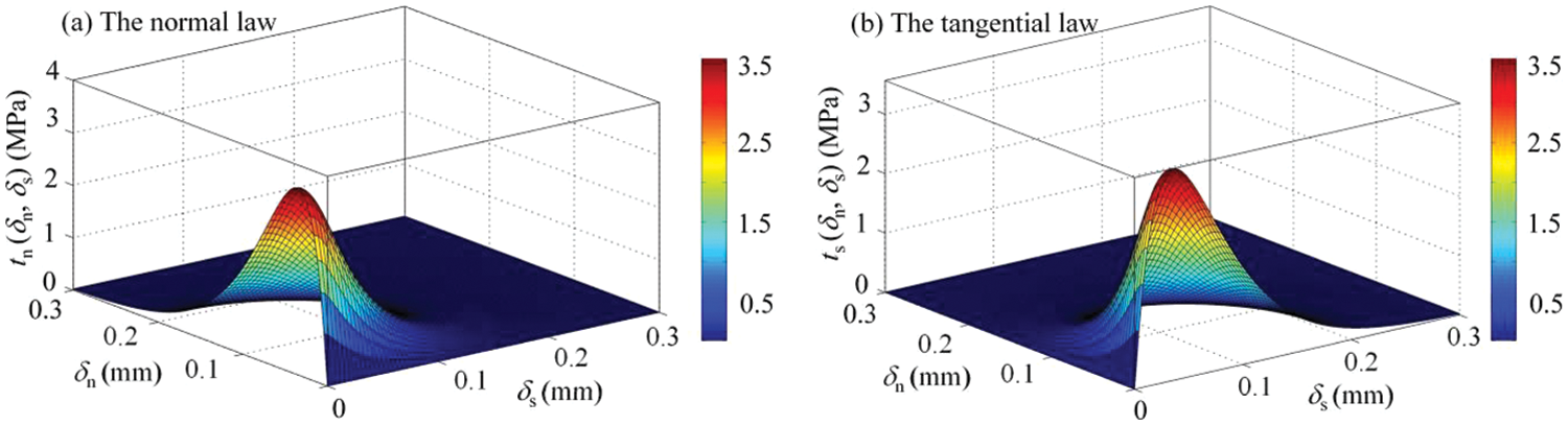
Figure 4: The 3D schematic diagram for the traction separation law under a tension-shear state

Concerning the compression-shear mode, a compression-shear-coupled law, derived from the Mohr-Coulomb strength theory, is established for the tangential direction of the discontinuous surface,

tsc=βexp⁡(1)τpδsδcexp⁡(−β|δs|δc)(|δs|≤δsr,for strength softening stage)(9a)

tsc=rcτp(|δs|>δsr,for residual strength stage)(9b)

where |⋅| represents the absolute value function; δsr serves as the threshold value distinguishing the softening and residual stages of the CZM; τp denotes the peak strength of the discontinuous surface, defined as

τp=βσt+μs|tn|(10)

rc represents a reduction coefficient applied to the interface peak strength to align it with its residual strength, while μs denotes the frictional coefficient along the discontinuous surface (Here μs = tanϕp, ϕp is the peak frictional angle on the crack surface).

Furthermore, the normal expression is formulated based on a penalty stiffness method aimed at preventing the self-penetration of the cracked surfaces, i.e.,

tn=αexp⁡(1)σtδcδn(11)

wherein α is a factor adjusting the value of the penalty stiffness.

Similarly, Fig. 5 presents a 3D schematic diagram illustrating the traction-separation law under a compression-shear state. In the tn-δn-δs coordinate system, the normal law is depicted as a plane, with the normal traction increasing linearly as the negative (or compressive) displacement increases. In contrast, the tangential law exhibits a nonlinear relation before reaching its threshold value δsr, resembling those given in Fig. 4. However, the peak traction increases with the rise of compressive displacement due to the incorporation of Mohr-Coulomb strength theory. Furthermore, the tangential law transitions to a linear relation once the crack surface enters the residual strength state.

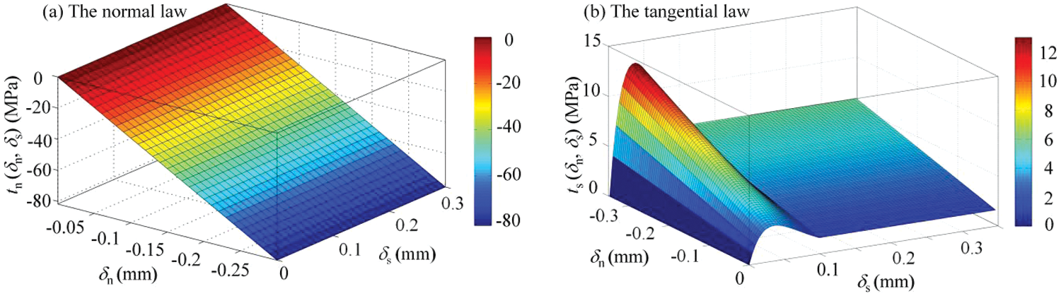
Figure 5: The 3D schematic diagram for the traction separation law under a compression-shear state

3  Model Implementations and Validations

3.1 Model Implementations

In this study, the N-AFEM utilized an ABAQUS user-defined element (UEL). Furthermore, a zero-thickness 2D linear cohesive element, which is formulated from the coupled CZM (as illustrated in Section 2.3), is developed as a UEL subroutine within the N-AFEM, enabling effective incorporation of tension-compression-shear coupling for localized bands in geomaterials into the numerical method.

Concerning crack initiation and growth, this study employs a hyperbolic law in the tn-ts space as the crack initiation criterion [17,27], represented by Eq. (12).

f(tn,ts)=ts2−(c−tn⋅μs)2+(c−σt⋅μs)2(12)

Here tn and ts on the crack plane denote the normal and shear stresses, respectively, of elements on the specific plane (i.e., crack surface) before cracking. The model parameters c (=βσt), μs, and σt, are assumed to be consistent with those of the continuum before elements start cracking. Eq. (12) serves a role similar to the Mohr-Coulomb yield surface in classical plasticity. In simpler terms, when the averaged stress of the Gauss integration points within an element reaches a certain state f(tn,ts)=0, the element initiates cracking in a prescribed direction expressed as Eq. (13).

θ=45∘+φ′/2(13)

where θ represents the angle between the crack surface and the direction of the minimum principal stress; φ′denotes the angle determined by the tangent direction of the hyperbolic curve based on Eq. (12) at the crack initiation point.

3.2 Model Validation

In this section, we validate the coupled CZM’s accuracy under compression-shear conditions using the direct shear test. Additionally, we analyze the correlation between the CZM parameters and the strength parameters of geomaterials to demonstrate its applicability in geotechnical structures. Tensile behaviors were previously scrutinized and validated in our prior work based on the clay beam test [20]; therefore, we omit its repetition here.

To emulate the direct shear test conducted by [28], a model is established in this subsection. As illustrated in Fig. 6, the model measures 60 mm in length and 30.4 mm in height, delineated by a phantom dotted line into two segments: the upper and lower boxes. The upper box undergoes a constant normal pressure P (20, 53, 100, and 200 kPa) on its top surface and prescribed displacement ux on its side surfaces, while the lower box faces fixed and horizontal constraints on its bottom and side surfaces, respectively. Consequently, under these conditions, the upper and lower boxes slide along the phantom dotted line (see Fig. 6), inducing soil rupture.

Figure 6: Schematic diagram of the direct shear model

The structured mesh, employing a four-node quadrilateral linear element, was used for both the upper and lower boxes, while zero-thickness cohesive elements derived from the coupled CZM were positioned along the phantom dotted line. Material parameters for this model were determined through the iterative fitting of numerical predictions to experimental data: Young’s modulus E = 1.2 + 0.6P (MPa), Poisson’s ratio ν = 0.3, β = 1.0, peak internal friction angle ϕp = 38.66° (μs = tanϕp = 0.176), residual internal friction angle ϕr = 32.62°(rc = tan(ϕr)/tan(ϕp) = 0.8), δsr = 0.566 mm, δc = 1.2 mm. Given the sandy soil nature of this model, the tensile strength σt was set to zero (i.e., cohesion c = βσt = 0). To prevent self-penetration of crack surfaces, a normal contact stiffness of kn = 1.13 × 109 kN/m3 was assigned to the CZM.

Fig. 7 illustrates the comparison between numerically predicted curves of average shear stress (τxy) vs. tangential displacement (ux) and experimental results, where τxy is an average from the tangential stress of all cohesive elements along the shear slip surface. Additionally, Fig. 7 displays the predicted results based on the CZM without compression-shear coupling. It can be seen that the curves obtained from the coupled CZM closely resemble the experimental outcomes. In contrast, the four curves derived from the uncoupled CZM consistently align with the abscissa of Fig. 7, suggesting this model does not factor in the contribution of normal pressure to the interfacial shear strength of materials.

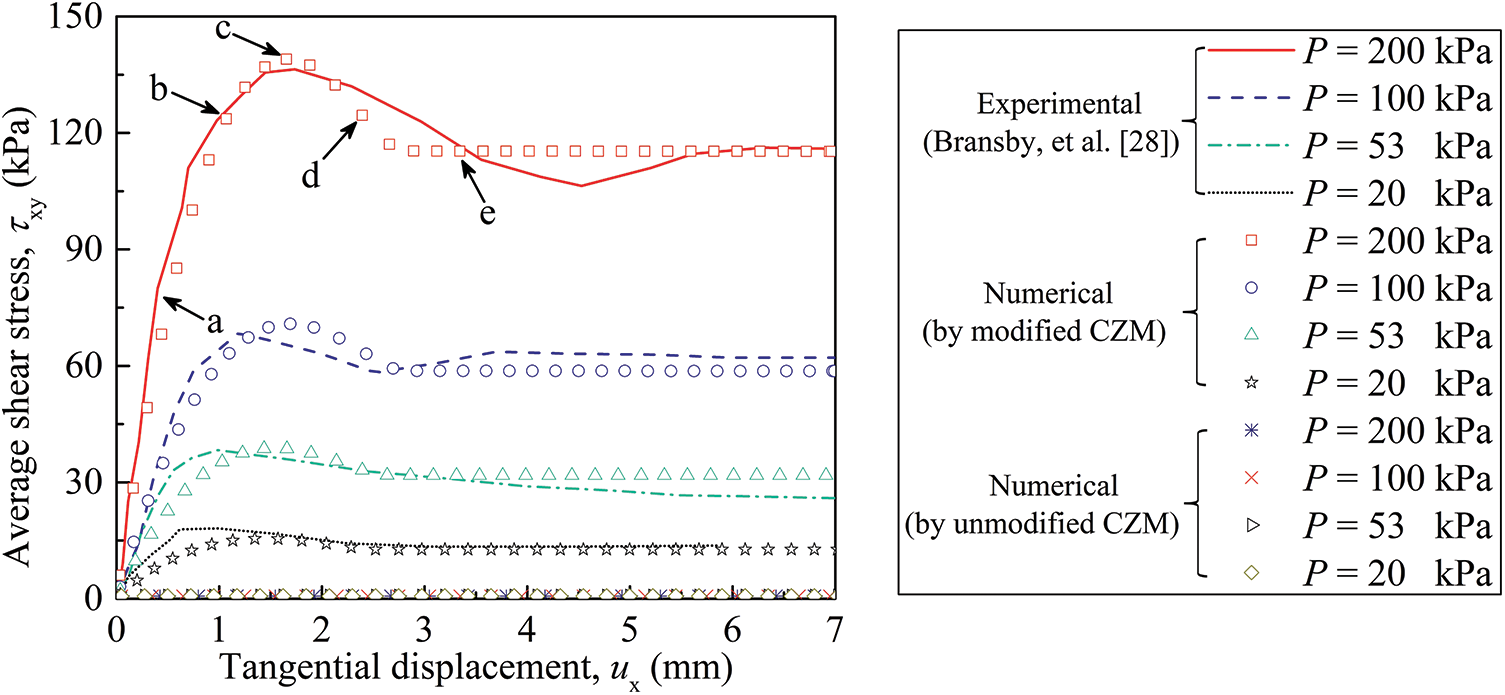
Figure 7: The comparison between shear stress vs. tangential displacement curves obtained from numerical simulations and experimental data

Fig. 8 elaborates on the stress evolution within the direct shear model, portraying shear stress images corresponding to five loading stages identified in Fig. 7 (i.e., stages a to e). The direct shear model exhibits progressive failure, showcasing evident strain localization. Initially (Figs. 8a and 8b), both ends of the potential slip surface reach the peak material strength, indicated by shear cracks in this region. Subsequently, due to the continuous increase in tangential displacement (ux), shear cracks further propagate from the ends towards the center section of the slip surface (see Figs. 8c and 8d). By stage e (Fig. 8e), the direct shear model has undergone propagation by the shear crack, entering a residual state with reduced shear stress observed in this image. Both the response curves and staged stress images provide preliminary evidence supporting the coupled CZM’s applicability in describing geomaterial cracking under a compressive-shear state.

Figure 8: Stress contours of the direct shear model under undeformed meshes: (a) to (e) corresponding to five loading stages identified in Fig. 7 (unit: MPa)

4  Plane Strain Slope Stability

4.1 Model and Parameters

This section employs the N-AFEM to model a two-dimensional soil embankment based on studies by [16] and [29] (as depicted in Fig. 9). This aims to validate the proposed method’s reliability and uncover the localized deformation and failure mechanisms within the clayey soil slope. Considering the embankment’s symmetry, half of it is considered in the calculation model, featuring a rigid rectangular foundation subject to a vertical displacement uy simulating an external load (F denotes the reaction force from uy). The model’s geometric dimensions and boundary conditions are outlined in Fig. 9, where multiple fixed constraints are applied to the model’s bottom, and horizontal forced constraints are placed on the right edge. The model assumes a plane strain condition, and its material parameters align with the provided references: E = 10 MPa, ν = 0.4, ϕp = 10° (μs = 0.176), ϕr = 1.718° (rc = 0.17), σt = 32 kPa, c = βσt = 32 kPa, δsr = 0.00335 m and δc = 0.05 m. A four-node, quadrilateral plane element is used in this model, and the total number of elements is 4900 (= 70 × 70), as shown in Fig. 9.

Figure 9: The discretized slope model and its boundary conditions

4.2 Validation for Numerical Method

In this section, we validate the effectiveness of the proposed numerical framework by comparing our predicted results with those from existing numerical models. Fig. 10 presents a comparison of rupture band trajectories obtained from the A-FEM model (this study), the AES (assumed enhanced strain) model with no opening-sliding coupling [29], and the AES model with opening-sliding coupling [16]. The three models exhibit similar rupture characteristics, encompassing overall trajectories, rupture initiation points, and rupture outcropping points. Notably, the A-FEM model demonstrates more consistent rupture band trajectories with those from the work of [16]. This consistency can be attributed to introducing an opening-sliding cohesive model into the AES model, as we also integrate a similar tension-compression-shear model CZM into the A-FEM algorithm. Additionally, we compare a quantitative parameter, the maximum reaction force at the loading point (see Fig. 9), among the three models: Fmax equals 817.64 kPa [29], 805.88 kPa (this study), and 716.43 kPa [16]. Considering both rupture characteristics and peak reaction force, it is evident that the proposed numerical framework performs well in simulating the failures of soil slope models and can be employed for subsequent simulations.

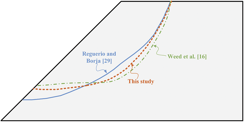
Figure 10: A comparison of the rupture band trajectories based on the various numerical models

4.3 Failure Mode of Soil Slope with Tension-Shear Considered

This sub-section delves into analyzing the failure mode of a clay soil slope. Figs. 11a–11f illustrate the evolution of rupture bands within the slope via maximum principal strain contours at different loading stages. Initially (Fig. 11a), deformation concentrates beneath the foundation surface, evidenced by a series of strain bubbles. Subsequently, as vertical displacement (uy) continues, a rupture band initiates at the bottom right of the rigid foundation, resulting in a nearly straight-line slip (Fig. 11b). Based on the zoomed picture at the right side of Fig. 11b, it is evident that the maximum principal stress at this stage consistently points downward to the left. This observation implies that soils neighboring the slip line are predominantly in a tension-shear state. Furthermore, when combined with the crack growth direction (refer to Eq. (13)), it provides additional insights into the rationale behind the development of a nearly straight-line slip during the initial crack stage. However, with further uy increase, the main rupture band’s trajectory shifts from a straight line to an arc, propagating from the inclined edge of the model (Figs. 11c and 11d). We attribute the rupture band trajectory shift to the rotation of the maximum principal stress directions. This is evident from the fact that the maximum principal stress in this area exhibits varying directions (refer to the zoomed picture in Fig. 11d). Besides, the change in principal stress direction at this stage also signifies soils near the arc-shaped sliding surface experience compression-shear failure. Stages e and f (Figs. 11e and 11f) show the sliding mass moving along the cut-through rupture band, displaying evident relative displacement with the sliding bed. The maximum principal stress near the slip line has undergone a transition from a downward-left direction to an upper-right direction. This transition results in a further “cocking-up” of the rupture band at the end (refer to the zoomed picture in Fig. 11f). In summary, the slope exhibits straight-lined and arc-shaped rupture trajectories under tension-shear and compression-shear states, respectively.

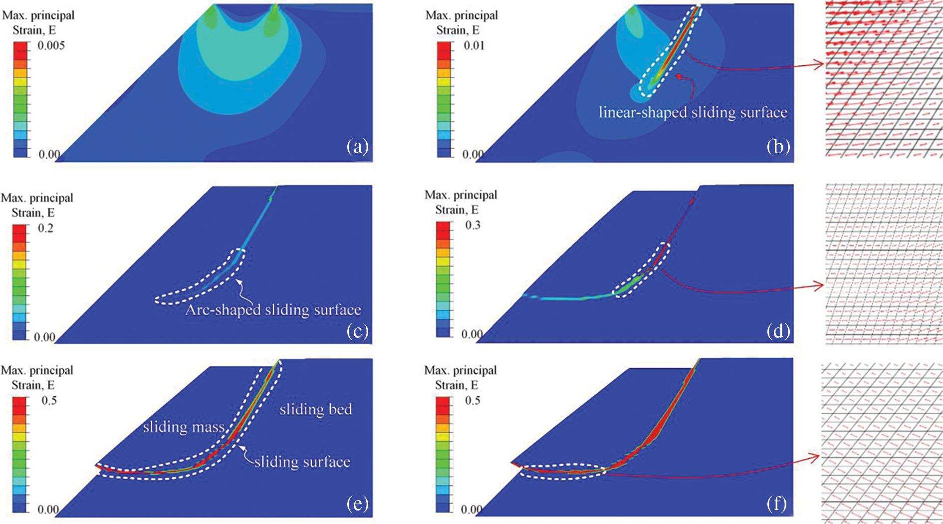
Figure 11: The maximum principal strain contours of the slope model under various loading stages

Fig. 12 illustrates the displacement evolution in this model, represented by the symbol ‘U’ denoting the resultant displacement. Based on the results, the slope deformation is categorized into three processes: I, II, and III. Process I indicates no rupture on the slope, with displacement primarily under the rigid foundation (Fig. 12a). In process II, tension-shear failure initiates on the right side of the foundation, resulting in a notable discontinuity of displacement on the rupture surface. The resultant displacement focuses mainly on the inverted triangle region to the left of the slip surface and beneath the foundation (Figs. 12b–12d). This unique displacement distribution potentially contributes to the rupture band’s propagation under tension-shear loading. Process III displays a layered displacement distribution gradually increasing from shallow to deep (Figs. 12e and 12f), with the largest displacement observed in the sliding surface, indicating the rigid motion of the slide body. These findings offer new insights into the distinct deformation and progressive failure pattern showcased by the slope experiencing a combination of tension-shear and compression-shear states.

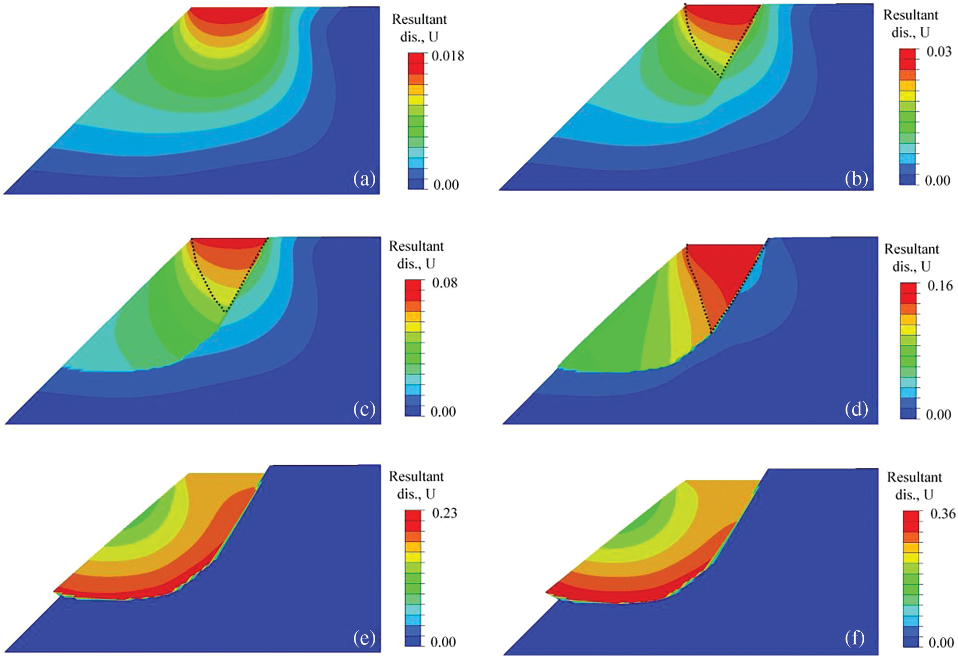
Figure 12: The resultant displacement contours of the slope model under various loading stages

4.4 Effect of Tensile Strength in Soils

This section aims to investigate the impact of soil tensile strength on a clay soil slope by varying the parameter σt within the range of 15, 25, 32, 42, and 50 kPa. Fig. 13 displays the propagation trajectories of rupture bands depicted in principal strain contours. The observations indicate an upward movement of the rupture band in the slope corresponding to an increase in the tensile strength of the CZM, accompanied by a proportional reduction in its overall scale. Moreover, these strain contours illustrate that heightened tensile strength correlates with a weakening of compression-shear deformation, as evidenced by a shorter compression-shear slip line. This observation aligns with findings associated with slopes exhibiting tension cracks.

Figure 13: The maximum principal strain contours of the slope model under various tensile strengths

In Fig. 14a, the reaction force is plotted against vertical displacement curves for the slope model at various tensile strengths, and the peak values of these curves are presented in Fig. 14b. The response curves demonstrate a consistent trend: the reaction force gradually increases before reaching its peak with imposed displacement uy, followed by a dramatic decrease after the peak due to complete rupture band propagation. However, both the peak reaction force and the corresponding displacement increase with higher tensile strength (see Fig. 14b). These findings suggest that (1) the peak point in the response curves can help distinguish the slope’s state to some extent, and (2) slopes with higher tensile strength tend to exhibit improved bearing capacity and stability. Regarding the latter phenomenon, we attribute it to the implementation of the coupled CZM, wherein the fracture energy of materials is proportionate to their tensile strength. As the tensile strength increases, the energy dissipation required to form a unit surface area of the fully separated crack inevitably rises. This suggests that more external energy (or work) is necessary for the slope. From a macroscopic perspective, this reflects an enhancement in the capacity and stability of slopes.

Figure 14: The response curves of the slope model with various tensile strengths: (a) reaction force vs. vertical displacement curve; (b) peak force (displacement) vs. vertical displacement curve

4.5 Effect of Weighting Factor β

This section presents a comparative analysis of the weighting factor (β) within the coupled CZM to elucidate the influence of tension-shear and compression-shear cohesive laws on soil slope deformation and failure patterns. Fig. 15 illustrates a comparison of rupture band propagation paths in slopes with varying weighting factors: β values of 0.6, 0.8, 1.0, 1.2, and 1.4. Notably, an increase in β from 0.6 to 1.4 corresponds to the downward movement of the sliding surface, an elongation of the total propagation path, and a reduction in the relative distance between the shear head point and the slope bottom, decreasing from 5.03 to 1.26 m. Moreover, an escalated weighting factor results in a transition of the initial propagation section of the slip surface from an approximately straight line to a smoother arc, which is attributed to the slope failure mode. For models with smaller weighting factors, the initial slip surface propagation is primarily characterized as pure tension or tension-shear failure. Hence, the propagation path appears approximately linear. Conversely, larger weighting factors emphasize the role of tangential CZM, inducing distinct shear failure accompanied by an arc-shaped slip surface. Fig. 16 further depicts the relationship between the peak reaction force and the weighting factor. As the weighting factor increases, the slope model exhibits a higher peak reaction force. This finding suggests that the extension of the compression-shear segment due to increased weighting factors contributes to greater slope stability.

Figure 15: The maximum principal strain contours of the slope model under various weighting factors

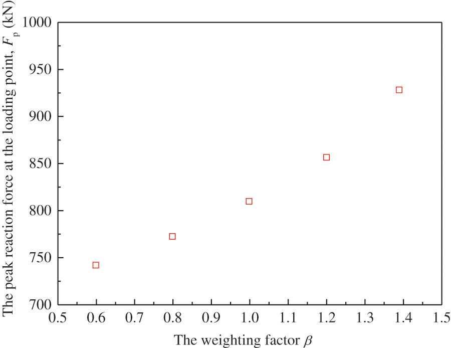
Figure 16: The peak reaction force vs. the weighting factor curve of the slope model

4.6 Effect of Interlayer in Soil Embankment

The highway subgrade is a soil body structure comprising a natural earth foundation and an artificial fill embankment. These components typically exhibit varying stiffness throughout their depth due to construction techniques and geostatic stress. Addressing this variability, a simplified embankment, derived from the previously analyzed soil slope, was extensively studied here by incorporating various Young’s moduli for the soil layers. Fig. 17 illustrates the embankment models, including homogeneous soil (model A), stratified soil (model B), soft interlayer soil (model C), and hard interlayer soil (model D), each identified by their corresponding Young’s modulus in the schematic diagram.

Figure 17: Soil slope model with interlayer: (a) model A with homogeneous soil; (b) model B with stratified soil; (c) model C with a soft interlayer; (d) model D with a hard interlayer

Fig. 18 presents a comparison of the deformation and failure patterns among four slope models using principal strain contours at the initial and failure stages. At the initial stage, model A, featuring homogeneous soil, displays a smoother strain bubble (Fig. 18a). Conversely, models B, C, and D exhibit strain discontinuities within strain bubbles due to abrupt Young’s modulus interfaces. The strain bubble in model B diminishes as Young’s modulus increases with depth (Fig. 18b). Contrastingly, model C exhibits strain expansion within the soft interlayer owing to a sharp decrease in Young’s modulus (Fig. 18c). In model D, the strain bubble gradually disappears along the depth, particularly at the upper surface of the hard interlayer, suggesting a mitigating effect on soil deformation. These findings suggest that deformation primarily occurs in layers with lower modulus, while hard interlayers limit deformation, potentially reducing geohazard risks in slopes.

Figure 18: The principal strain contours of soil slope at initial and failure stages

Additionally, strain contours at the failure stage illustrate notable differences in the failure patterns of the four slope models. Models B and D exhibit shorter rupture bands, shifting the outcrop location upward compared to model A (Figs. 18e, 18f and 18h). Model C follows a similar rupture band path as model A, but within the hard interlayer, its geometric profile diverges notably from models A, B, and D. For model C, as the rupture band propagates from the initial soil layer to the soft interlayer, its growth trajectory changes from a downward convex arc to an upward convex arc (Fig. 18g). However, as the rupture band moves from the soft interlayer to the next soil layer, the trajectory adjusts from an upward convex arc to a downward convex shape. A similar shift occurs in model D when the rupture band propagates between the hard and soft interlayers. These characteristics suggest that deformation parameters, such as modulus, significantly influence slope stability by altering the failure pattern. Moreover, the rupture band generally transitions from a downward convex to an upward convex arc while moving between the hard and soft interlayers, exhibiting the opposite adjustment when moving from the soft interlayer to the hard interlayer.

5  Conclusions

The study introduces an integrated algorithm within the finite element framework to explore fracture damage (or cracking) in cohesive materials and the relevant geohazard mechanisms. Demonstrating the validity of the coupled CZM using existing experimental data, we combined this model with the N-AFEM to analyze how tensile properties affect soil slope landslides. Key findings are outlined as follows:

(1) Geohazard development from localized deformation exhibits progressive failure and strong discontinuities. Integrating CZM and N-AFEM accurately reproduces these features, capturing complex compression-shear and tension-shear coupling behaviors within rupture bands.

(2) Cohesive soil slopes with tension-shear failures show straight-lined rupture paths, while compression-shear slopes exhibit arc-shaped paths. Increased soil tensile strength enhances stability and bearing capacity, minimally impacting rupture paths. Higher weighting factors lead to more compression-shear ruptures, improving slope stability.

(3) Soil modulus significantly influences slope stability, altering failure patterns. Slopes with interlayers show rupture band trajectories that transition from downward to upward convex arcs when moving from hard to soft layers, and transition oppositely when moving from soft to hard layers.

Acknowledgement: The authors express gratitude to Li-min Chen for his valuable contribution to the enhancement of this paper, particularly in figure preparation and numerical modeling.

Funding Statement: This research was supported by Zhejiang Provincial Natural Science Foundation of China under Grant Nos. LQ23E080001 and LTGG23E080002, National Natural Science Foundation of China under Grant No. 12272334, and Zhejiang Engineering Research Center of Intelligent Urban Infrastructure (No. IUI2023-YB-07).

Author Contributions: Study conception and design: Chengbao Hu, Shilin Gong, Zhongling Zong; data collection: Chengbao Hu, Xingwang Bao, Xiaojian Ru; analysis and interpretation of results: Chengbao Hu, Shilin Gong, Zhongling Zong, Xingwang Bao; draft manuscript preparation: Chengbao Hu, Shilin Gong, Bin Chen. All authors reviewed the results and approved the final version of the manuscript.

Availability of Data and Materials: Some or all data and models that support the findings of this study are available from the corresponding author upon reasonable request.

Conflicts of Interest: The authors declare that they have no conflicts of interest to report regarding the present study.

References

1. Bishop, A. W. (1955). The use of the slip circle in the stability analysis of slopes. Géotechnique, 51, 7–17. [Google Scholar]

2. Baker, R., Garber, M. (1978). Theoretical analysis of the stability of slopes. Géotechnique, 28(4), 395–411. [Google Scholar]

3. Matsui, T., San, K. C. (1992). Finite element slope stability analysis by shear strength reduction technique. Soils and Foundations, 32(1), 59–70. [Google Scholar]

4. Griffiths, D. V., Lane, P. A. (1999). Slope stability analysis by finite elements. Géotechnique, 49(3), 387–403. [Google Scholar]

5. Wang, X. N., Yu, P., Yu, J. L., Yu, Y. Z., Lv, H. (2018). Simulated crack and slip plane propagation in soil slopes with embedded discontinuities using XFEM. International Journal of Geomechanics, 18(12), 04018170. [Google Scholar]

6. Xu, G. J., Zhong, K. Z., Fan, J. W., Zhu, Y. J., Zhang, Y. Q. (2020). Stability analysis of cohesive soil embankment slope based on discrete element method. Journal of Central South University, 27(7), 1981–1991. [Google Scholar]

7. Chen, Z., Song, D. Q. (2021). Numerical investigation of the recent Chenhecun landslide (Gansu, China) using the discrete element method. Natural Hazards, 105, 717–733. [Google Scholar]

8. Gong, S. L., Hu, C. B., Guo, L. X., Ling, D. S., Chen, G. Q. et al. (2022). Extended DDA with rotation remedies and cohesive crack model for simulation of the dynamic seismic landslide. Engineering Fracture Mechanics, 266, 108395. [Google Scholar]

9. Ray, R., Deb, K., Shaw, A. (2019). Pseudo-spring smoothed particle hydrodynamics (SPH) based computational model for slope failure. Engineering Analysis with Boundary Elements, 101, 139–148. [Google Scholar]

10. Conte, E., Pugliese, L., Troncone, A. (2019). Post-failure stage simulation of a landslide using the material point method. Engineering Geology, 253, 149–159. [Google Scholar]

11. Gong, S. L., Ling, D. S., Chen, G. Q., Niu, J. J., Hu, C. B. (2020). Remedies for distortion and false volume expansion problems with large rotation in discontinuous deformation analysis. International Journal of Geomechanics, 20(11), 04020216. [Google Scholar]

12. Bao, Y. D., Li, Y. C., Zhang, Y. S., Yan, J. H., Zhou, X. et al. (2022). Investigation of the role of crown crack in cohesive soil slope and its effect on slope stability based on the extended finite element method. Natural Hazards, 110, 295–314. [Google Scholar]

13. Geng, D. J., Dai, N., Guo, P. J., Zhou, S. H., Di, H. G. (2021). Implicit numerical integration of highly nonlinear plasticity models. Computers and Geotechnics, 132, 103961. [Google Scholar]

14. Liu, P. F. (2015). Extended finite element method for strong discontinuity analysis of strain localization of non-associative plasticity materials. International Journal of Solids and Structures, 72, 174–189. [Google Scholar]

15. Motamedi, M. H., Weed, D. A., Foster, C. D. (2016). Numerical simulation of mixed mode (I and II) fracture behavior of pre-cracked rock using the strong discontinuity approach. International Journal of Solids and Structures, 85, 44–56. [Google Scholar]

16. Weed, D. A., Foster, C. D., Motamedi, M. H. (2017). A robust numerical framework for simulating localized failure and fracture propagation in frictional materials. Acta Geotechnica, 12, 253–275. [Google Scholar]

17. Hu, C. B., Yang, Q. D., Ling, D. S., Tu, F. B., Wang, L. et al. (2021). Numerical simulations of arbitrary evolving cracks in geotechnical structures using the nonlinear augmented finite element method (N-AFEM). Mechanics of Materials, 156, 103814. [Google Scholar]

18. Vo, T. D., Pouya, A., Hemmati, S., Tang, A. M. (2017). Numerical modelling of desiccation cracking of clayey soil using a cohesive fracture method. Computers and Geotechnics, 85, 15–27. [Google Scholar]

19. Barani, O. R., Mosallanejad, M., Sadrnejad, S. A. (2016). Fracture analysis of cohesive soils using bilinear and trilinear cohesive laws. International Journal of Geomechanics, 16(4), 04015088. [Google Scholar]

20. Hu, C. B., Wang, L., Ling, D. S., Cai, W. J., Huang, Z. J. et al. (2020). Experimental and numerical investigation on the tensile fracture of compacted clay. Computer Modeling in Engineering & Sciences, 123(1), 283–307. https://doi.org/10.32604/cmes.2020.07842 [Google Scholar] [CrossRef]

21. de Maio, U., Gaetano, D., Greco, F., Lonetti, P., Nevone Blasi, P. et al. (2023). The reinforcing effect of nano-modified epoxy resin on the failure behavior of FRP-plated RC structures. Buildings, 13(5), 1139. [Google Scholar]

22. Liu, W., Schesser, D., Yang, Q. D., Ling, D. S. (2015). A consistency-check based algorithm for element condensation in augmented finite element methods for fracture analysis. Engineering Fracture Mechanics, 139, 78–97. [Google Scholar]

23. Park, K., Paulino, G. H. (2012). Computational implementation of the PPR potential-based cohesive model in ABAQUS: Educational perspective. Engineering Fracture Mechanics, 93, 239–262. [Google Scholar]

24. Xu, X. P., Needleman, A. (1994). Numerical simulations of fast crack growth in brittle solids. Journal of the Mechanics and Physics of Solids, 42(9), 1397–1434. [Google Scholar]

25. Ortiz, M., Pandolfi, A. (1999). Finite-deformation irreversible cohesive elements for three-dimensional crack-propagation analysis. International Journal for Numerical Methods in Engineering, 44(9), 1267–1282. [Google Scholar]

26. Camacho, G. T., Ortiz, M. (1996). Computational modelling of impact damage in brittle materials. International Journal of Solids and Structures, 33(20–22), 2899–2938. [Google Scholar]

27. Carol, I., Prat, P. C., López, C. M. (1997). Normal/shear cracking model: Application to discrete crack analysis. Journal of Engineering Mechanics, 123(8), 765–773. [Google Scholar]

28. Bransby, M. F., Davies, M. C. R., Nahas, A. E., Nagaoka, S. (2008). Centrifuge modeling of reverse fault-foundation interaction. Bulletin of Earthquake Engineering, 6(4), 607–628. [Google Scholar]

29. Regueiro, R. A., Borja, R. I. (2001). Plane strain finite element analysis of pressure sensitive plasticity with strong discontinuity. International Journal of Solids & Structures, 38(21), 3647–3672. [Google Scholar]