A Dynamic Prediction Approach for Wire Icing Thickness under Extreme Weather Conditions Based on WGAN-GP-RTabNet

1  Introduction

Transmission lines are critical for the power system, responsible for the transport and distribution of electrical energy, and influential in socio-economic development and stability of daily life. However, most transmission lines are in the wild environment without adequate protective measures, making them vulnerable to various natural factors. Particularly, wire icing, a severe natural disaster, not only leads to incidents such as conductor galloping, insulator flashovers, and tower collapses, but also results in widespread power outages, causing significant economic losses and severe disruption of people’s daily lives. Wire icing is one of the ice disasters that poses a major threat to the safe operation of transmission lines, leading to accidents such as conductor galloping, insulator flashover, and tower collapses [1]. Traditional ice monitoring methods mainly rely on manual inspection and image monitoring, which have the problems of high labor intensity and long consumption [2]. To improve the monitoring efficiency, online monitoring systems based on image recognition and stress analysis have been developed, which can monitor the wire icing in real time and realize automatic warnings by image processing technology [3]. In addition, the ice monitoring method based on capacitance measurement has been proposed and proved to be feasible in practical applications through experimental research [4]. Random forest and WRF models have been used to predict wire icing thickness, and the accuracy and stability of prediction are improved significantly by Bayesian parameter optimization [5]. Fig. 1 shows ice-covered wires in cold weather.

Figure 1: Manual inspection of ice-covered wires

The grey prediction model has been widely used to predict wire icing thickness. By analyzing the correlation between micrometeorological parameters (such as ambient temperature, relative humidity, wind speed, and direction) and wire icing thickness, an effective prediction model has been established [6]. By collecting transient traveling wave signals and calculating their arrival time, wire icing thickness can be accurately measured by the transient traveling wave detection method of the Hilbert-Huang transform [2]. In the natural ice-covered environment, the wire icing thickness of the eight-split wires increases nonlinearly with time [7]. When the wire is covered by light freezing fog, the ice-covered roughness increases and the density decreases. Formulas for the stress, sag, and length of ice-covered conductors based on the catenary theory have been derived in [8]. A numerical model of wire icing thickness under comprehensive load conditions has been established by sag variation and temperature measurement [7]. Moreover, it has been verified that the maximum relative error between the calculated value and the measured value in this model is 10.7%.

At the present stage, more wire icing thickness prediction and monitoring methods have been proposed, such as measuring icing thickness based on a binocular vision camera and accurately calculating icing thickness combined with traveling wave positioning technology [2,6]. A method for calculating icing thickness using infrared imagery has been proposed in [9]. A risk assessment model for heavily iced power transmission lines based on a multilayer feedforward deep neural network (MLF-DNN) has been proposed in [10]. The ice load monitoring system based on a fiber Bragg grating sensor is also used to calculate the icing thickness of transmission lines, and its stability and accuracy in harsh environments are verified by field experiments [11]. To cope with complex and changeable meteorological conditions, a prediction method of wire icing thickness based on a multivariate grey prediction model has been developed. In addition, the accuracy of this model is improved via grey correlation analysis [6].

Nowadays abundant achievements have been made in the research of transmission line icing issues, including the formation mechanism of icing, online monitoring technology, and icing thickness prediction models. These studies provide important theoretical and technical support for improving the ice resistance capability of power grids. However, ice disaster is still one of the major threats to safe operation of power grids, especially in extreme weather conditions. Monitoring data will appear to be distorted, greatly increasing the prediction error of icing thickness. In addition, in the actual working environment, there is still incomplete monitoring equipment, failing to obtain detailed data. Therefore, it is still necessary to further study and optimize the ice cover identification and prediction model, as well as to develop a model that is more adaptable to the actual production environment.

This paper proposes a method of wire icing thickness identification and measurement based on discrimination by deep learning and calculation by a mechanical model. The WGAN-GP framework is used to upsample the original ice monitoring data, and the cyclic neural network encodes the historical environmental information into a message vector. Subsequently, the RTabNet model assesses the ice-covered state of wires. Then, according to the tension-temperature relation of wires and the deformation coordination equation, the mechanical calculation model of wire icing thickness is derived. The main contributions of the paper are as follows:

1. We propose a dynamic predictive model for estimating wire icing thickness, which remains robust under extreme weather conditions. The model uses GAN to generate synthetic data and can achieve satisfactory training outcomes even with limited original data.

2. We combine deep learning with a mechanical model. Compared with traditional methods, our method encodes historical environmental information and judgment results into message vectors. It also integrates the RTabNet model to accurately assess the ice-covered state. Moreover, it removes the wind-induced tension from the ice-wind coupling tension, enabling a more precise measurement of the icing thickness of wires.

3. We evaluate our model by using ice-covered data from a region in Xinjiang, China. The results show that our model is more accurate than several traditional models. It is less affected by wind-induced effects than the traditional mechanical models.

2  GAN

2.1 GAN Model

Generative Adversarial Networks (GANs), introduced by Goodfellow et al. [12] in 2014, are widely used to generate data distributions that approximate real-world distributions. A GAN consists of a generator, denoted by G, and a discriminator, denoted by D, trained in an adversarial manner. The basic structure of GAN is shown in Fig. 2. The generator creates synthetic samples G (z) from a noise vector z, while the discriminator distinguishes real samples x from generated ones. The training process optimizes the following objectives:

minGmaxDV(D,G)=Ex∼pdata(x)[lg⁡D(x)]+Ez∼pz(z)[lg⁡(1−D(G(z)))].(1)

Figure 2: GAN structure diagram

This adversarial setup allows G to generate samples that progressively align with the true data distribution pdata(x). However, traditional GANs often suffer from challenges like mode collapse and unstable training, particularly in complex scenarios like generating ice-covered wire data.

2.2 WGAN-GP

To address the limitations of traditional GANs, Wasserstein GAN (WGAN) replaces the Jensen-Shannon divergence with the Wasserstein distance to measure the discrepancy between real and generated distributions [13]. The Wasserstein distance is defined as

W(pr,pg)=infγ∈∏(pr,pg)E(x,y)∼γ[‖x−y‖].(2)

where Pr and Pg represent the real and generated data distributions, and ∏(pr,pg) is the set of joint distributions with marginals Pr and Pg.

WGAN-GP [14] further improves this approach by introducing a gradient penalty term to ensure the Lipschitz continuity of the discriminator D, defined as

LGP=Ex^∼Px^(x^)[(‖∇x^D(x^)‖2−1)2].(3)

where x^ is sampled along straight lines between real and generated samples.

The training process alternates between optimizing the discriminator and generator objectives.

Discriminator Loss:

LD=Ex∼Pdata(x)[D(x)]−Ez∼Pz(z)[D(G(z))]+λEx^∼Px^(x^)[(‖∇x^D(x^)‖2−1)2].(4)

Generator Loss:

LG=−Ez∼Pz(z)[D(G(z))].(5)

The combined optimization goal is to alternately minimize LG and maximize LD, aligning the generated data distribution Pg with the real data distribution Pr. This adversarial setup ensures that G learns to produce synthetic samples that closely mimic the real data. At this point, the optimization problem of training GAN is converted to

minGmaxDV(D,G)=Ex∼Pdata(x)[D(x)]−Ez∼Pz(z)[D(G(z))]+λEx^∼Px^(x^)[(‖∇x^D(x^)‖2−1)2].(6)

2.3 Data Augmentation of the Ice-Covered Wires Generated Based on the WGAN-GP Data

The WGAN-GP framework is employed to generate synthetic ice-covered wire data to address the scarcity of observational datasets. The data augmentation process involves the following steps:

1. A noise vector z∼Pz(z) is fed into the generator G, which produces synthetic samples G(z) matching the dimensionality of real data.

2. The generator and discriminator are alternately trained to optimize LG and LD, and aligning the generated data distribution Pg with the real data distribution Pr.

3. The trained generator produces m batches of synthetic samples, and the top n samples with the highest similarity (Combined evaluation of Wasserstein distance and Jensen-Shannon divergence) to real data are selected to form the augmented dataset. The process is shown in Fig. 3.

Figure 3: Flow chart of GAN training

This augmented dataset enriches the training pool for downstream tasks, such as training the RTabNet classifier. As demonstrated in Section 5, the generated data closely aligns with real-world distributions, validated by metrics such as Wasserstein distance and t-SNE visualizations.

3  An Ice-Covered State Discrimination Model Based on RTabNet

To efficiently identify whether the wires are in an ice-covered state and to eliminate misjudgment of the ice-covered state of the wires under the influence of a strong wind environment, this section adopts an ice-covered state discrimination model based on RTabNet, which adds the Long Short-Term Memory (LSTM) network to encode historical environmental monitoring data and discrimination results into a message vector. Combined with real-time environmental monitoring data, the model evaluates the true state of wires and issues early warning alerts at different levels based on the severity of the wire icing.

The data on ice-covered wires in the extreme environment is relatively complex. If the Decision Tree (DT)-based method is adopted, a lot of processes of feature engineering are required, which is not conducive to providing timely feedback of monitoring status [15]. RTabNet, as a deep neural network model for processing table data, retains the advantages of traditional DNN and utilizes the idea of a DT-based method [16].

For the judgment of the state of ice-covered wires, RTabNet can directly input the raw monitoring data without any data preprocessing operations. Training based on gradient descent can be easily integrated into the end-to-end model.

Due to the approximate hyperplane boundary of tabular data, the DT method can usually obtain better results. RTabNet first uses the multiplication coefficient mask matrix to select the input features. After linear transformation, the elements that meet the conditions are zeroed by the Rectified Linear Unit (ReLU) function. Finally, the results are added and output by the Softmax function. The constructed network structure can realize the DT-like output manifold and can learn sparse instance-level feature selection from data with the advantage of the DT method. The learning ability of the model can be improved by nonlinear processing [17]. The DT-like diagram is shown in Fig. 4.

Figure 4: DT-like diagram

A sequential attention mechanism is used to mimic the flow of the DT method [18], as shown in Fig. 5. The whole model is composed of multiple submodules of the same decision steps. Step i inputs the information from (i−1) and decides which feature to use. The output features are aggregated into the overall decision.

Figure 5: Feature selection diagram of WGAN-GP-RTabNet. Two decision blocks are used as examples to separately process features related to environmental factors and sensors to predict ice-covered levels

The distinction between instantaneous wind misjudgment and wire icing lies in the fact that, during icing, the environmental temperature and humidity of the wire must meet the conditions necessary for ice formation. Therefore, the model needs to be able to identify the relevant features. RTabNet has instance-level feature selection, with local and global interpretability. The model uses a learnable mask for the soft selection of significant features [19]. Through this sparse selection, the learning ability of the decision-making step is concentrated on the significant features, such as temperature and humidity, thereby improving the model’s learning efficiency. At the same time, the mask can show the selected features in each decision step and the contribution degree of the feature of a single sample to the step. Feature selection of all decision steps will finally be aggregated and reflect the relative importance of each step in the final decision, as shown in Fig. 6. Attentive transformers are used to obtain the following masks:

M[i]=Sparsemax(P[i−1]⋅hi(a[i−1])).(7)

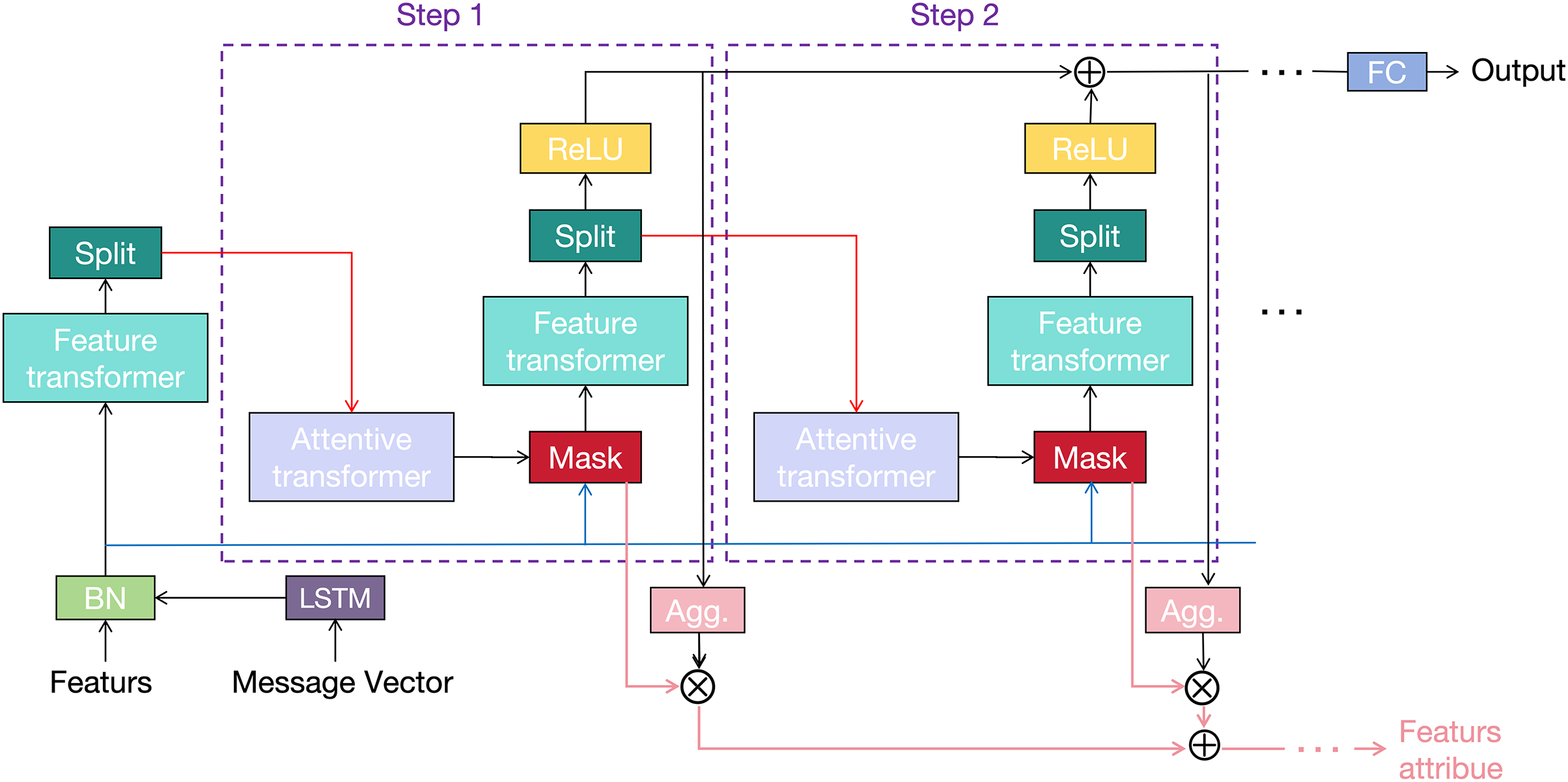
Figure 6: Coding structure of WGAN-GP-RTabNet

Note that ∑j=1DM[i]b,j=1, hi is a trainable function, P[i] is a priori scale term indicating the extent to which the feature has been used before, P[i]=∏j=1i(γ−M[j]), and γ is the relaxation parameter.

In feature processing, feature transformers are used to process the selected features and to segment the output of the decision step and subsequent information. The first half of the feature transformer is responsible for calculating common features, and parameters are shared in all steps. The personality characteristics are calculated in the second half, and the parameters are updated only in the current step. This structure improves the robustness of the model.

Due to the impact of instantaneous wind, the environmental monitoring data of adjacent periods is prone to show large differences, which can lead to incorrect judgments. Therefore, we use the LSTM model to encode the historical environmental monitoring data and the output of the classifier into a message vector. The structure of this component is shown in Fig. 7. In the tth period, the classifier receives the current environmental characteristic data xt and historical message vector ot−1, and outputs the classification result yt. The historical message component will generate a new historical message vector ot based on the environment feature data xt, output results yt and the historical message vector of the previous time ot−1 as input. Its update method is as follows:

ot=LSTM(xt,yt,ot−1;θhm).(8)

Figure 7: Structure of WGAN-GP-RTabNet

Note that xt is the environmental monitoring data at time t, yt is the classification result, ot−1 is the historical message vector, and θhm is the attenuation coefficient, which is used to control the weight of new input information and historical information.

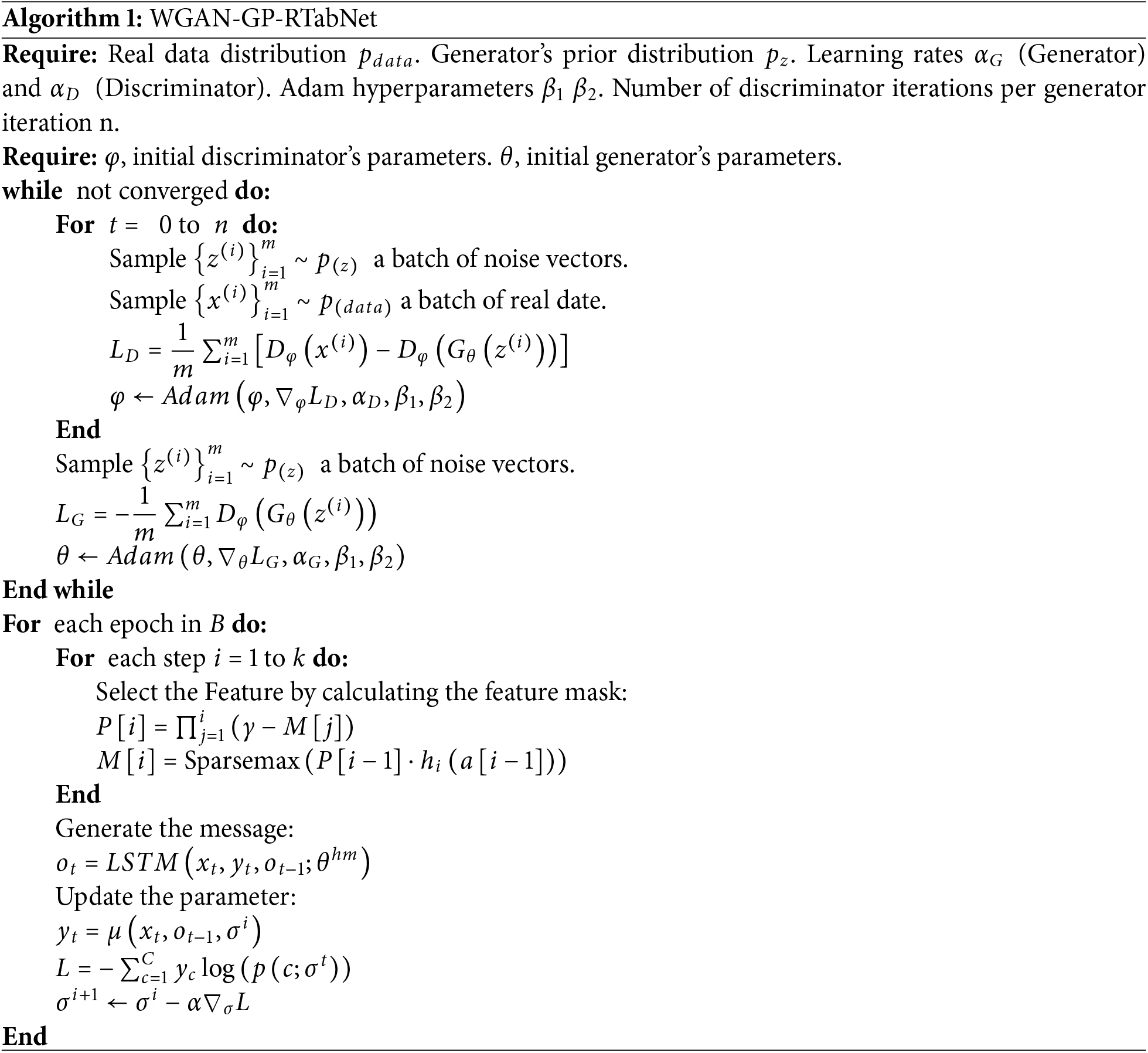
The training process is shown in Algorithm 1. We divide data into mini batches to update the parameters and obtain a generator to extend the data set. At each training step, we use a learnable mask to select the significant features and update parameters, The specific process is shown in Fig. 8.

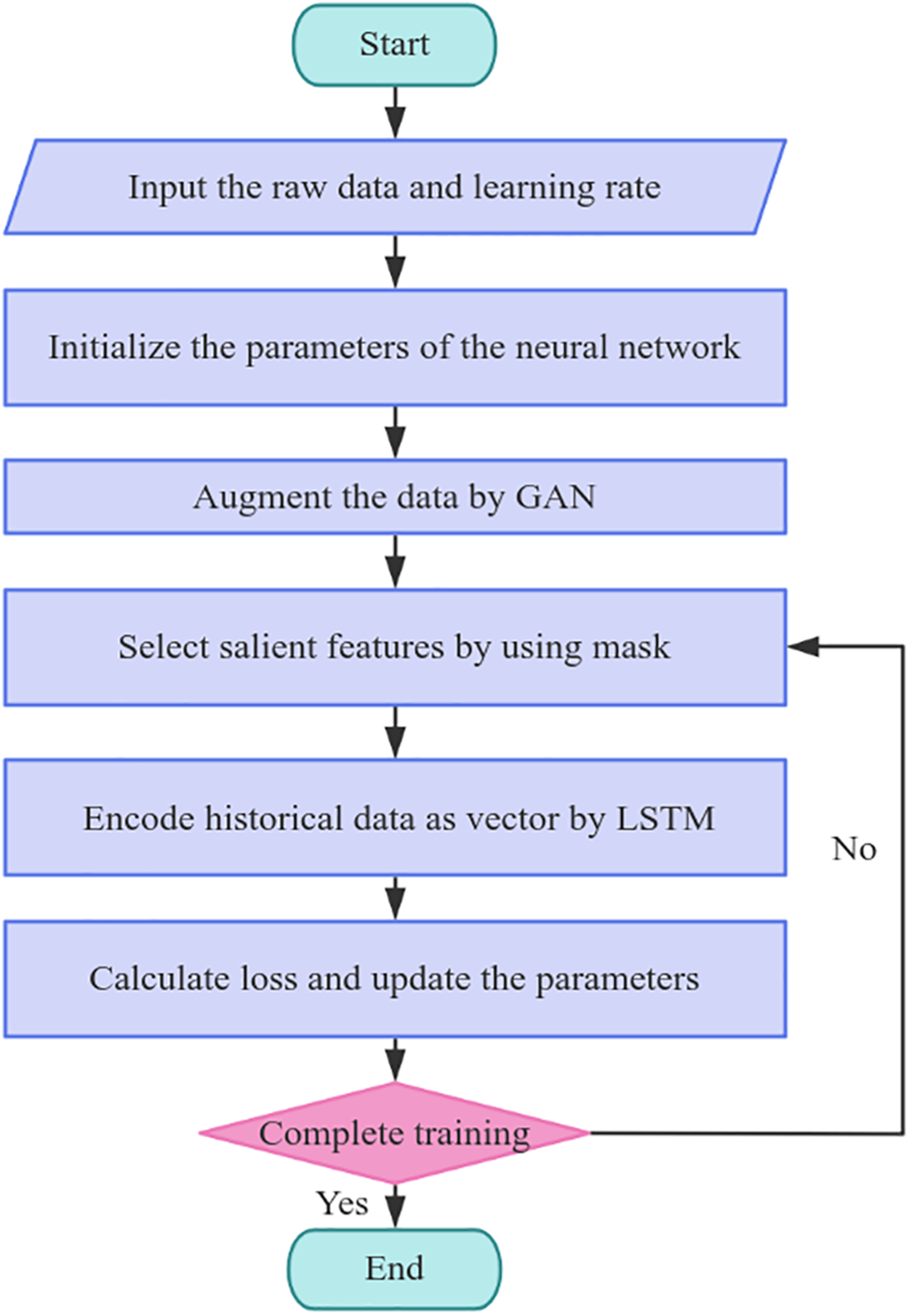
Figure 8: Training procedure of the WGAN-GP-RTabNet

4  Dynamic Prediction of Wire Icing Thickness

In this section, based on the identification of ice-covered wires using the WGAN-GP-RTabNet model, we use a mechanical model of wire icing thickness by combining the relation among temperature, wire elongation, and wire tension [20]. If it is identified that the change in wire tension is affected by instantaneous wind, no warning information will be issued. If it is identified that the change in wire tension is caused by ice covering, the mechanical model is used to calculate the wire icing thickness.

We chose to use a parabolic configuration. A section of a wire is cut out for unit force analysis, as shown in Fig. 9a. Assume that the horizontal component of tension at a point of the wire is Fx1=F0 and the vertical component is Fz1=F0tan⁡θ. For uniformly ice-covered wires [21], it can be approximated that wires are only subject to vertical loads, and according to the static equilibrium conditions of wires, it holds that

d2zdx2=−q+q0F0.(9)

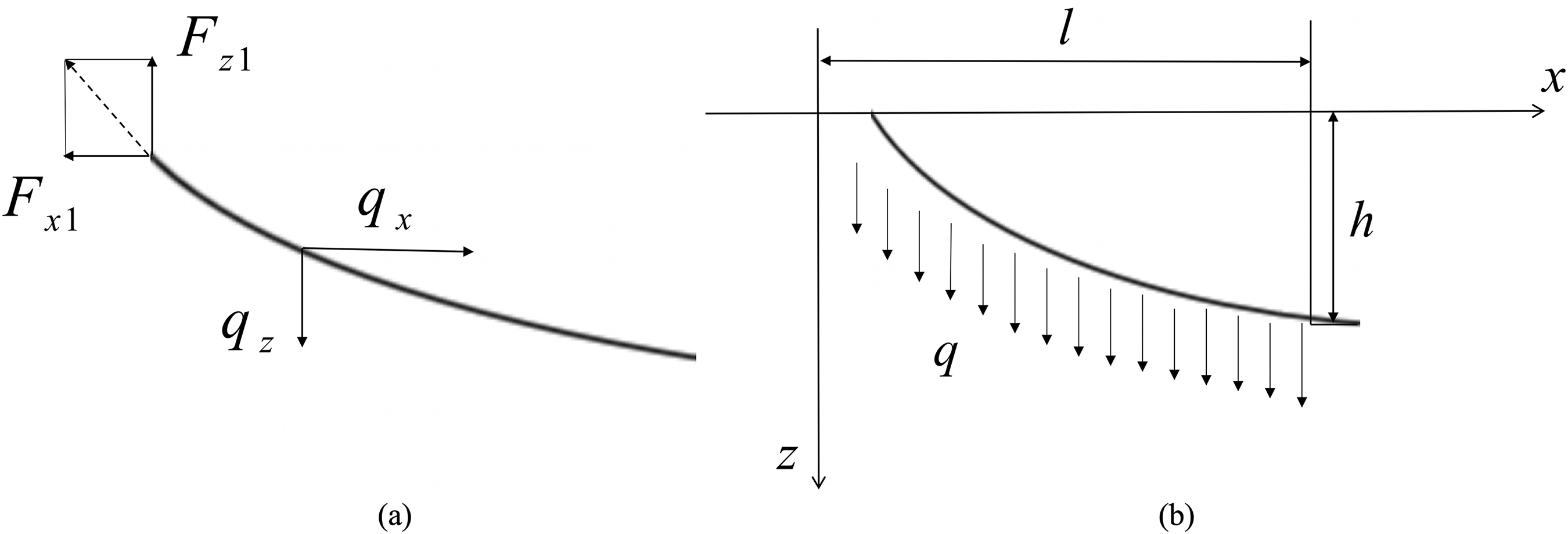
Figure 9: Stress analysis diagram. (a) Stress analysis of wire unit; (b) Distribution of ice load along the wire

In this formula, q is the ice load, q0 is the deadweight loads, and F0 is the horizontal tension of the wire.

Assuming that the ice load is uniformly distributed along the wire, as shown in Fig. 9b. Let the displacements of the wire along the x axis and the z axis be u and w, respectively. When the wire unit reaches the final state [22], the total elongation of the wire is

ΔS=∫sΔs=∫L[12(dwdx)2+dzdxdwdx]dx.(10)

The elongation of the wire is related to the change of tension and temperature [23]. The total elongation of the wire is

ΔS=∫0L(ΔFEA+αΔt)ds=∫0L(ΔFEAdsdx+αΔt)dsdxdx.(11)

In this formula, E is Young’s modulus (Pa), ΔF is the change of horizontal tension of the conductor before and after icing (N), A is the cross-sectional area of the conductor is calculated (m2), α is the temperature expansion coefficient of the conductor, and Δt is the temperature change before and after icing (°C).

The wire finally satisfies the deformation coordination equation. The difference between the horizontal tension F1 of the wire after ice covering and the horizontal tension F0 of the wire before ice covering can be obtained according to the parabola formula:

ρiceπ((d+2hice)2−d24)g=24F12L2(ΔFEA+αΔt)+q02(1−F12F0)(12)

Note that d is conductor diameter and hice is the icing thickness.

The wind load per unit length of the wire is

qw=12ρv2CdD.(13)

Note that qw is the wind load, ρ is the air density (kg/m3), v is the wind speed (m/s), Cd is the aerodynamic drag coefficient, and D is the upwind length of the ice-covered wire (m).

In the presence of wind, under the combined effects of wind-ice load and self-weight load, the dynamic equation of the ice-covered wire is

F1d2ydx2+qw=0.(14)

Note that y is the displacement in the vertical direction (m).

In the absence of wind or under low wind speeds, wire icing thickness can be calculated using Eq. (12). After the wind begins, the mass of ice on wires does not increase significantly in a short period. The change in wire tension is only related to the instantaneous wind speed. Therefore, after calculating the instantaneous wind load using Eq. (13), wire icing thickness can be determined by solving Eqs. (12) and (14).

The overall workflow of the dynamic prediction approach for wire icing thickness is shown in Fig. 10. The electric transmission line monitoring system saves the sensor data to the database after receiving it, and the model extends the data through a generator and conducts offline training. The trained model parameters are transferred to the operational model. If it is determined that the wire is covered with ice, the icing thickness is calculated after excluding the tension caused by the wind, and the results are returned to the monitoring system.

Figure 10: Flow chart of dynamic prediction approach for wire icing thickness

5  Experimental Results

In this paper, the data of transmission lines in a region of Xinjiang was selected as the experimental object to test the accuracy of the model in identifying the ice-covered state and the calculation accuracy of wire icing thickness. The wire model is LGJ-630/45, the span is 300 m, and the insulator is the type I suspended glass insulator FC7P/146. The upper end of the insulator is fixed, the lower end of the insulator has a degree of oscillation freedom, and the suspension point has no height difference.

All case studies were conducted on the same computer device with an NVIDIA GeForce GTX 1650, Intel Core i7-9750H CPU, and 16 GB of RAM. The modeling and training of neural networks were conducted using PyTorch, leveraging the WGAN-GP framework to address the scarcity of ice-covered wire data. A multi-layer residual neural network [24] was designed as the generator, while a standard multi-layer neural network served as the discriminator. After iterative training, the generator was fine-tuned to produce synthetic ice-covered wire data that closely aligned with real-world observations, providing a diverse and realistic dataset for subsequent analysis.

The generator in this model is specifically designed to capture the intricate distributions of ice-covered wire data. It employs dense layers for dimensionality expansion, ReLU activations to introduce non-linearity, and Batch Normalization to ensure stable learning. Residual Blocks are integrated to enhance feature learning, allowing the generator to accurately model subtle ice accumulation patterns. The final output layer applies a Tanh activation function, producing realistic synthetic data that effectively reflects the characteristics of real-world observations.

The discriminator is designed to distinguish between real and synthetic data, incorporating Leaky ReLU activations to mitigate vanishing gradients and Batch Normalization with Dropout to enhance regularization. This architecture ensures robust performance in handling the variability of icing thickness and environmental conditions, contributing to stable convergence during training. By guiding the generator, the discriminator facilitates the production of high-fidelity synthetic data that closely replicates real-world scenarios.

To evaluate the performance of the trained generator, 50 sets of synthetic ice-covered wire data were produced. The quality of these samples was assessed using the Jensen-Shannon (JS) divergence, calculated against the original dataset. The JS divergence between the generated data of the 50 groups and the original dataset is shown in Fig. 11. The nine sets with the lowest JS divergence values (the lowest being approximately 0.02) were selected for further analysis and training of the RTabNet model. Fig. 12 presents a t-SNE visualization of one selected dataset, illustrating the close alignment of the synthetic and real data distributions. The clustering of data points indicates that the generator effectively captured the underlying patterns of the original data, ensuring its suitability for downstream tasks.

Figure 11: JS divergence between the generated data and the original dataset for 50 groups

Figure 12: t-SNE of generated data (a) and original data (b)

The Wasserstein distance between the generated and original datasets was evaluated across eight features and four categorical labels, as shown in Fig. 13. Distances ranged from approximately 0.01 to 0.05, indicating strong alignment between the generated and original data distributions. Most features exhibited minimal distances (e.g., 0.01, 0.02), demonstrating the model’s ability to replicate the original dataset’s structure accurately. Slightly higher distances (up to 0.05) were observed for specific features or labels, which may reflect subtle variations introduced during the generative process. These variations likely stem from the complexity of certain features or inherent noise in the dataset. However, all distances remained within an acceptable range, confirming the WGAN-GP model’s effectiveness in producing high-quality synthetic data suitable for downstream tasks.

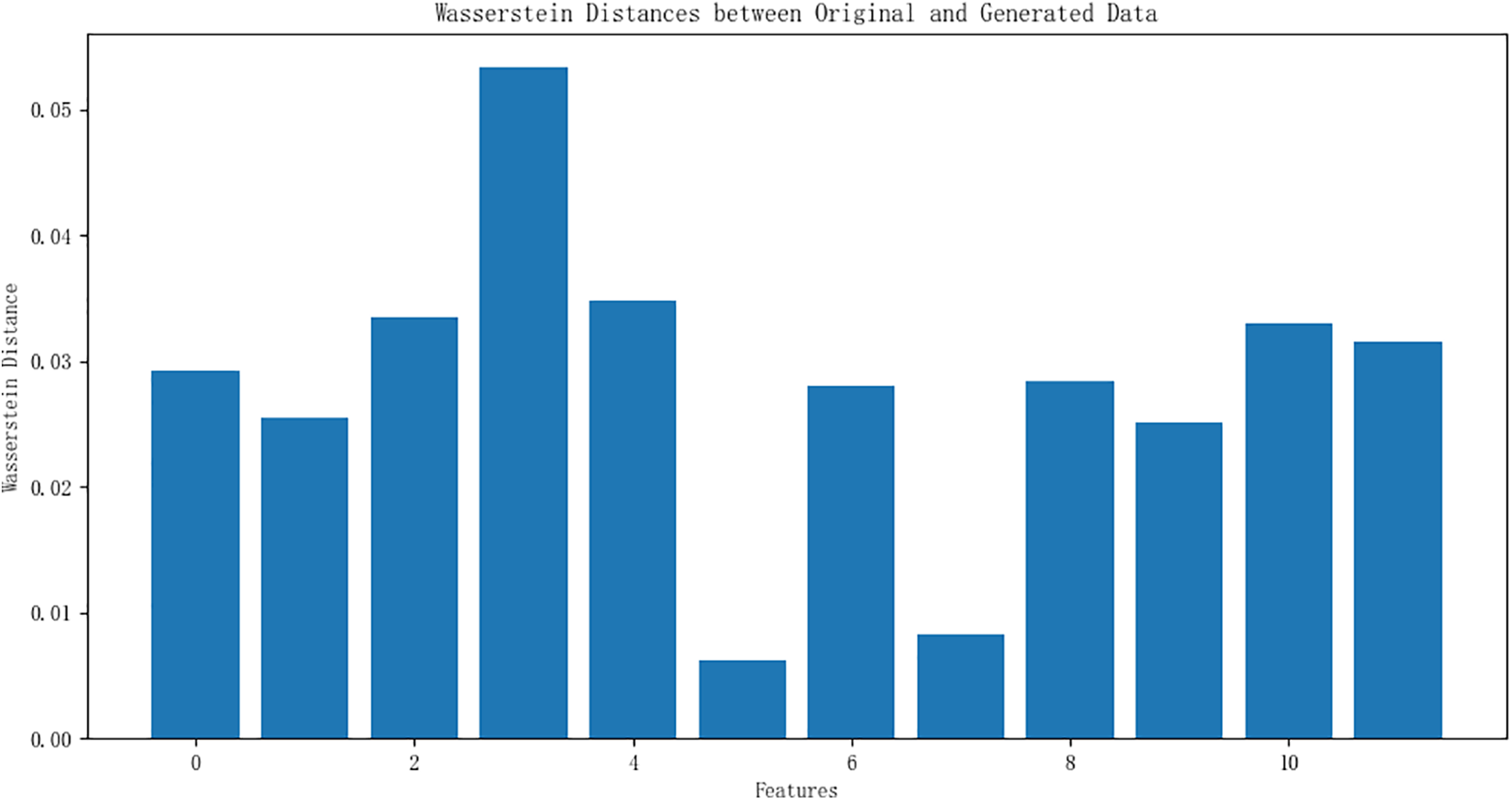
Figure 13: The Wasserstein distance between the generated and original datasets for 12 features, is represented on the x-axis by their corresponding feature indices. These indices correspond to the following features: 0. ‘Temperature’, 1. ‘Air humidity’, 2. ‘Wind speed’, 3. ‘Wind direction’, 4. ‘Atmospheric pressure’, 5. ‘Precipitation’, 6. ‘Pull value’, 7. ‘Tensile value datum’, 8. ‘Warning level_Normal’, 9. ‘Warning Level_Yellow Alert’, 10. ‘Warning Level_Orange Alert’, and 11. ‘Warning Level_Red Alert’

Correlation heatmaps for both the original and generated datasets, as shown in Fig. 14, reveal a high degree of consistency in feature relationships and categorical label associations. This consistency highlights the generative model’s ability to learn and reproduce the key statistical patterns of the original data. However, minor variations in correlation strength were observed, particularly for categorical labels such as “Warning Level_Normal,” where deviations in magnitude were evident. These discrepancies may result from the dataset’s complexity or suboptimal training conditions, such as mild overfitting or underfitting during the generative process. Despite these differences, the generated data closely reflects the overall structure of the original dataset, maintaining sufficient fidelity for use in RTabNet model training.

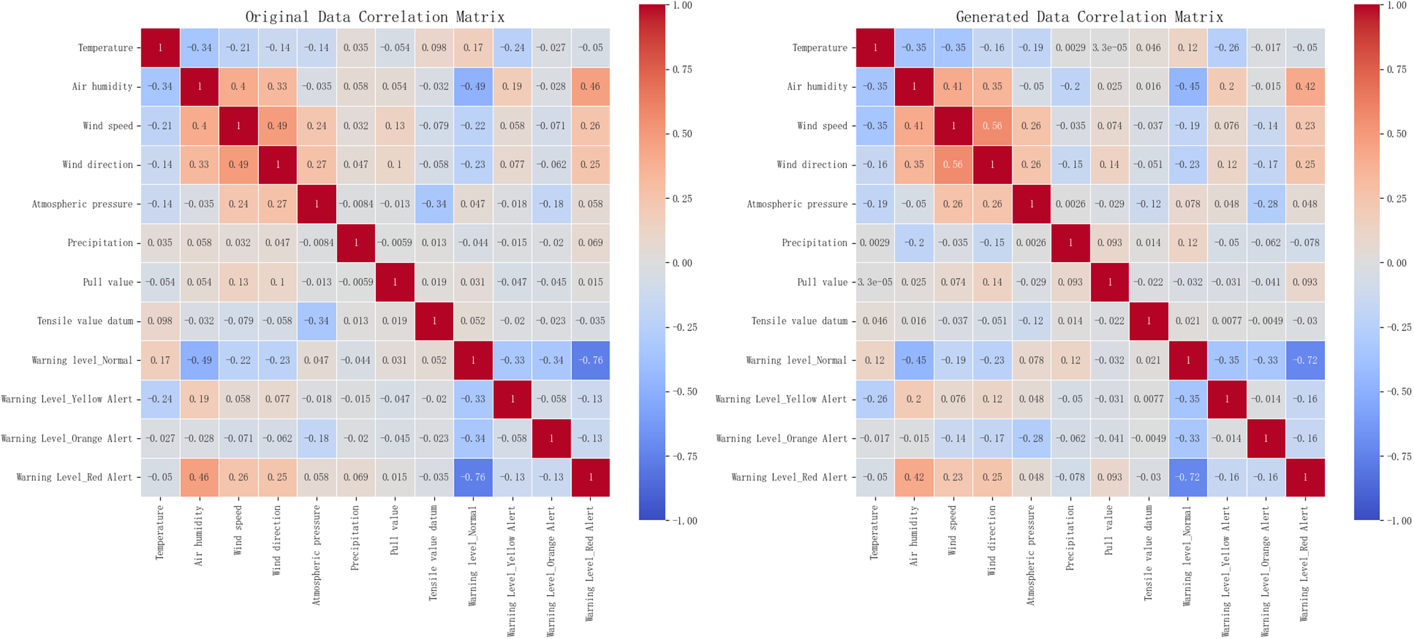
Figure 14: Correlation heatmaps

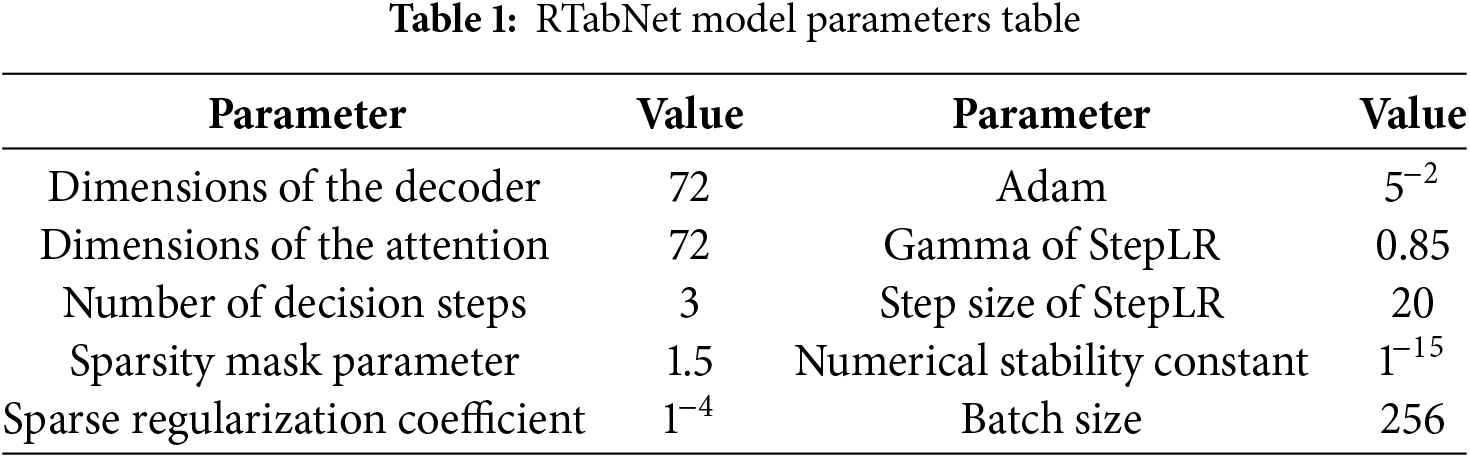
The effects of the RTabNet model and various parameters are shown in Table 1.

When we added the encoding structure based on LSTM into the framework, the accuracy of the model greatly improved compared with the baseline model, and it converged more quickly in the training process. The training result is shown in Fig. 15.

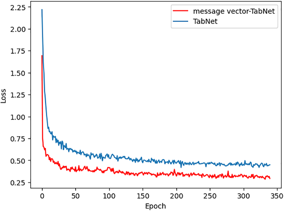
Figure 15: Comparison of the training loss

We evaluate the performance of the WGAN-GP-RTabNet model and other baseline models under four distinct weather cases: (1) Normal weather conditions, (2) Strong wind conditions, (3) Ice disaster conditions, and (4) Wind sensor failure. The results are summarized case by case as follows:

Case 1 (Normal weather conditions): Under normal weather conditions with calm or low wind speeds, icing thickness strongly correlates with temperature, humidity, and tension. In this case, the WGAN-GP-RTabNet model and baselines demonstrate similar accuracy in predicting wire icing states. However, the WGAN-GP-RTabNet model achieves slightly higher precision than the baseline models.

Case 2 (Strong wind conditions): We select historical data from monitoring stations in Xinjiang, where strong wind conditions were previously misclassified as wire icing events. As shown in Table 2, the WGAN-GP-RTabNet model achieves higher accuracy and precision compared to other baseline models. This also demonstrates the model’s ability to effectively determine wire states based on data characteristics.

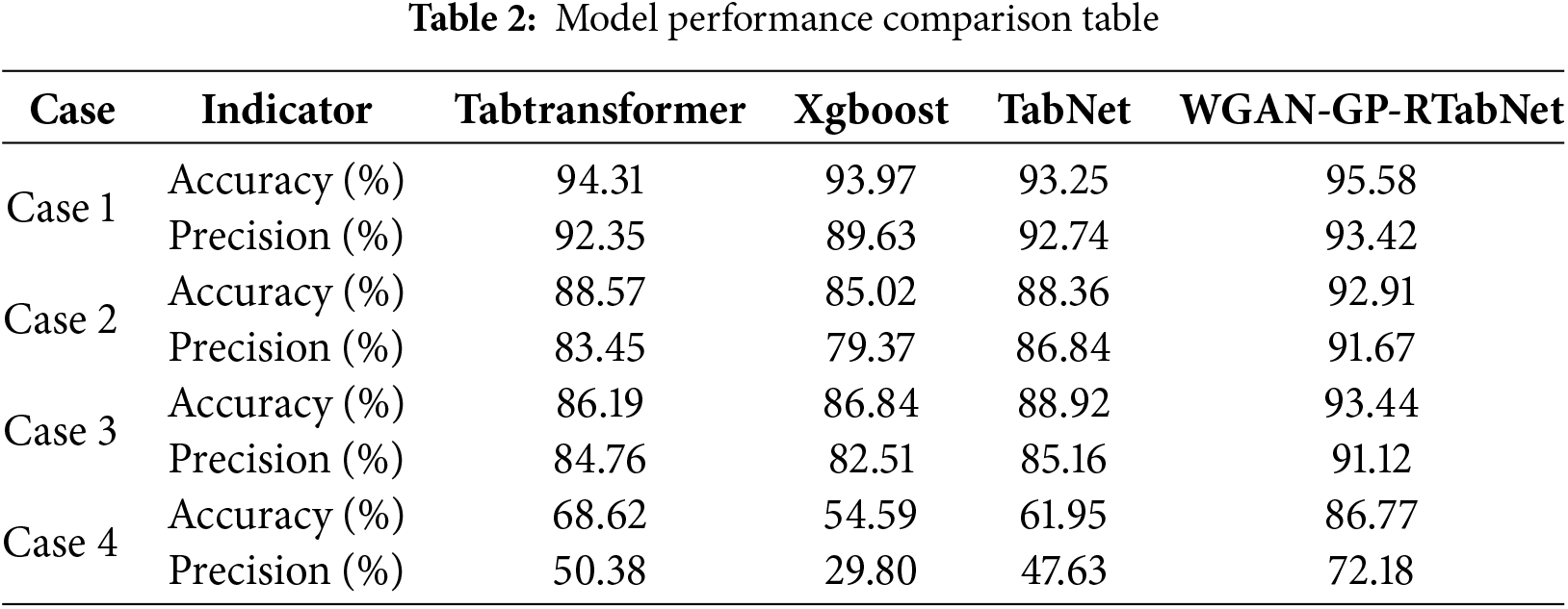
Case 3 (Ice disaster conditions): We test the models using data extracted from historical reports of ice disaster incidents, where the temperature ranges between −10°C and −20°C. As shown in Table 2, the WGAN-GP-RTabNet model achieves improved accuracy and precision compared to the TabNet model, highlighting its superior performance in extreme icing conditions.

Case 4 (Wind sensor failure): In extreme weather conditions, the wind speed sensor components of meteorological monitoring devices may freeze and fail when the temperature drops below −60°C. This failure causes wind speed and direction features to return constant values. To simulate this case, we insert constant values into the dataset. As shown in Table 2, the accuracy and precision of all models significantly decrease compared to normal conditions. However, the WGAN-GP-RTabNet model produces only a slight decline, demonstrating strong robustness under these adverse conditions.

Table 2 shows that the proposed WGAN-GP-RTabNet is superior to the traditional tree model, and the addition of GAN significantly improves the accuracy of judgment on the premise of improving the robustness of the model. The incorporation of a Recurrent Neural Network (RNN) effectively reduces the impact of rapid data fluctuations caused by strong transient winds. From the aggregate feature importance mask (Fig. 16), the WGAN-GP-RTabNet model only pays attention to valuable features, and the aggregate mask of irrelevant features is almost zero, which improves the interpretability and realizes the feature selection at the case level.

Figure 16: Mask matrix of the WGAN-GP-RTabNet model

From the mask matrix in Fig. 16, it can be observed that a feature mask matrix was constructed by selecting 30 sample data points and dividing the whole decision process into seven steps. Each decision step has a mask matrix with eight columns, representing the following eight features in sequence: air temperature, humidity, wind speed, wind direction, atmospheric pressure, rainfall, tension value, and tension reference value. The brighter the color, the higher the model’s attention to the corresponding feature for that data sample at each decision step. The model has learned all the features across the seven decision steps, with a higher focus on the first four features in the sample data.

Fig. 17 illustrates the global mask matrix for all sample data, reflecting the model’s global attention to each feature at every decision step. From Fig. 17, it is evident that the WGAN-GP-RTabNet model accurately selects effective features as the criteria for judging the ice-covered state. Temperature, air humidity, wind speed, and wind direction (i.e., the first four features) have a great influence on ice-covered wires. The above features are selected as the key learning objectives in the initial and final decision-making steps. In the intermediate steps, try to select other features, so that the model can focus on learning the features with significant influence based on ensuring the effective use of data features, which greatly improves the learning efficiency of the model.

Figure 17: Global mask matrix of the WGAN-GP-RTabNet model

Fig. 18a shows the growth of icing thickness over a day when an ice disaster occurs on a power transmission line in a region of Xinjiang and the icing thickness calculated by the model. The maximum error between the actual value and the calculated value of the model is 3.7%, which can be used to calculate the wire icing thickness more accurately. Combined with Fig. 18b, when the temperature of the transmission line is below 0°C and the humidity is above 92% rh, the transmission line is prone to be ice-covered.

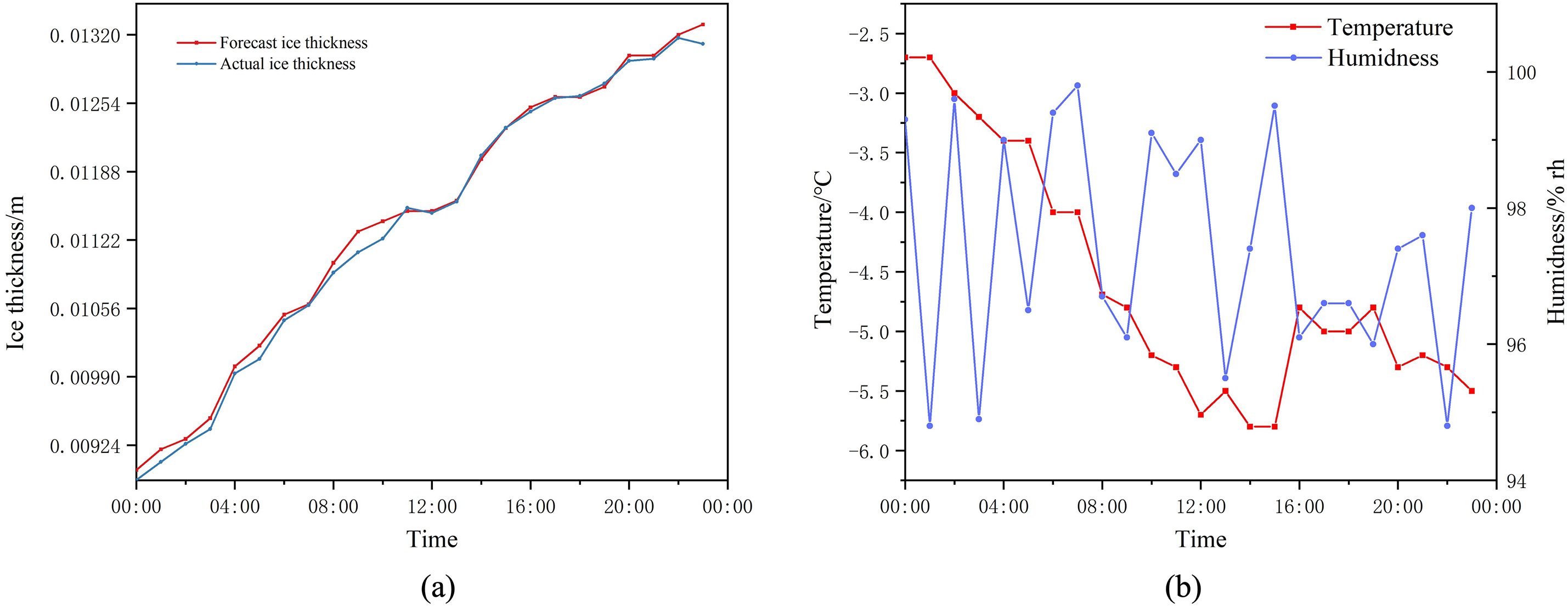
Figure 18: Comparison between actual and predicted icing thickness

6  Conclusion

In this paper, a method based on the combination of the WGAN-GP-RTabNet discrimination model, and the icing thickness mechanical calculation model is proposed, which effectively solves the misjudgment about wire state caused by strong instantaneous wind in extreme weather conditions. After eliminating the influence of wind load on wires, the wire icing thickness is calculated according to the mechanical model. The specific conclusions of the case study are as follows:

(1) Compared with the traditional decision tree model, the WGAN-GP-RTabNet discriminant model has stronger robustness and interpretability and reduces the complicated processes of data preprocessing. At the same time, the accuracy of the model in the real environment data set is 91.41%, which is better than other models.

(2) Based on the deformation caused by ice load and self-weight load and combined with the influence of temperature, the calculation model of icing thickness is finally obtained through the coordination equation of traverse deformation. The maximum error between the actual value and the calculated value is 3.7%.

(3) By analysis of the environment in the ice disaster area, it is shown that when the monitored environment’s temperature is below 0°C and the relative humidity is above 92%, the probability of wire icing significantly increases.

In the follow-up research work, the timing of ice-covered wires will be considered, and the historical data of wires will be encoded, so that the model can judge the current state combined with the historical icing situation of wires, and the accuracy rate of the model will be mentioned.

Acknowledgment: The authors acknowledge the support from the Science and Technology Project of the State Grid Corporation of China. We are also thankful for the insightful comments from anonymous reviewers, which have greatly improved this manuscript.

Funding Statement: This research is supported by the Science and Technology Project of State Grid Corporation of China (SGXJDK00GYJS2400035).

Author Contributions: The authors confirm contribution to the paper as follows: study conception and design: Mingguan Zhao, Xinsheng Dong; data collection: Yang Yang, Meng Li; analysis and interpretation of results: Hongxia Wang, Shuyang Ma, Xiaojing Zhu; draft manuscript preparation: Mingguan Zhao, Rui Zhu. All authors reviewed the results and approved the final version of the manuscript.

Availability of Data and Materials: The data that support the findings of this study are available from the corresponding author, M. Z., upon reasonable request.

Ethics Approval: Not applicable.

Conflicts of Interest: The authors declare no conflicts of interest to report regarding the resent study.

References

1. Jiang X, Fan C, Xie Y. New method of preventing ice disaster in power grid using expanded conductors in heavy icing area. IET Gener, Transm Distrib. 2019;13(4):536–42. doi:10.1049/iet-gtd.2018.5258. [Google Scholar] [CrossRef]

2. Zeng X-J, Luo X-L, Lu J-Z, Xiong T-T, Pan H. A novel thickness detection method of ice covering on overhead transmission line. Energy Proc. 2012;14(1):1349–54. doi:10.1016/j.egypro.2011.12.1100. [Google Scholar] [CrossRef]

3. Zhao J, Yan B, Zhao J, Chen B. Icing monitoring system of transmission lines based on image and stress. In: 2018 2nd IEEE Conference on Energy Internet and Energy System Integration (EI2); 2018; Beijing, China. p. 1–4. [Google Scholar]

4. Huan H, Wang Y, Mao X, Zeng H, Niu W. Experimental study on icing monitoring method based on capacitance measurement for transmission lines. In: 2022 IEEE International Conference on High Voltage Engineering and Applications (ICHVE); 2022; Chongqing, China. p. 1–4. [Google Scholar]

5. Wang Q, Zhou S, Zhang H, Su H, Zheng W. Prediction of conductor icing thickness based on random forest and WRF models. In: 2021 International Conference on Intelligent Computing, Automation and Applications (ICAA); 2021; Nanjing, China. p. 959–62. [Google Scholar]

6. Zhao J, An K, Zhao J. Research on multi-variable grey prediction model for icing thickness. In: 2019 IEEE 3rd Conference on Energy Internet and Energy System Integration (EI2); 2019; Changsha, China. p. 754–8. [Google Scholar]

7. Ding J, Hu S, Li J, Liu L, Ma L, Niu S, et al. Study on the growth model of ice-covered conductors with eight-split under light icing of freezing fog. In: 2023 IEEE Sustainable Power and Energy Conference (iSPEC); 2023; Chongqing, China. p. 1–7. [Google Scholar]

8. Hu Y, Cai F, Xian R, Liu W, Zhao M. Shape finding of ice covered wire for overhead line based on finite element analysis. In: Proceedings of the 18th Annual Conference of China Electrotechnical Society; 2024; Singapore. p. 137–47. [Google Scholar]

9. Chang Y, Yu H, Kong L. Study on the calculation method of ice thickness calculation and wire extraction based on infrared image. In: 2018 IEEE International Conference on Mechatronics and Automation (ICMA); 2018; Changchun, China. p. 381–6. [Google Scholar]

10. Huang G, Wu G, Guo Y, Liang M, Li J, Dai J, et al. Risk assessment models of power transmission lines undergoing heavy ice at mountain zones based on numerical model and machine learning. J Clean Prod. 2023;415(1–2):137623. doi:10.1016/j.jclepro.2023.137623. [Google Scholar] [CrossRef]

11. Jiang X, Xiang Z, Zhang Z, Hu J, Hu Q, Shu L. Predictive model for equivalent ice thickness load on overhead transmission lines based on measured insulator string deviations. IEEE Trans Power Deliv. 2014;29(4):1659–65. doi:10.1109/TPWRD.2014.2305980. [Google Scholar] [CrossRef]

12. Goodfellow I, Pouget-Abadie J, Mirza M, Xu B, Warde-Farley D, Ozair S, et al. Generative adversarial nets. In: Advances in neural information processing systems. Red Hook, NY, USA: Curran Associates, Inc.; 2014. [Google Scholar]

13. Arjovsky M, Chintala S, Bottou L. Wasserstein generative adversarial networks. In: Proceedings of the 34th International Conference on Machine Learning; 2017. Vol. 70, p. 214–23. [Google Scholar]

14. Gulrajani I, Ahmed F, Arjovsky M, Dumoulin V, Courville AC. Improved training of wasserstein gans. In: NIPS’17: Proceedings of the 31st International Conference on Neural Information Processing Systems; 2017; Long Beach, CA, USA. p. 5769–79. [Google Scholar]

15. Aaboub F, Chamlal H, Ouaderhman T. Analysis of the prediction performance of decision tree-based algorithms. In: 2023 International Conference on Decision Aid Sciences and Applications (DASA); 2023; Annaba, Algeria. p. 7–11. [Google Scholar]

16. Humbird KD, Peterson JL, McClarren RG. Deep neural network initialization with decision trees. IEEE Trans Neural Netw Learn Syst. 2018;30(5):1286–95. [Google Scholar] [PubMed]

17. Arik SÖ, Pfister T. TabNet: attentive interpretable tabular learning. Proc AAAI Conf Artif Intell. 2021;35(8):6679–87. [Google Scholar]

18. Mott A, Zoran D, Chrzanowski M, Wierstra D, Rezende DJ. S3TA: a soft, spatial, sequential, top-down attention model. 2019 [cited 2024 Oct 30]. Available from: https://openreview.net/forum?id=B1gJOoRcYQ. [Google Scholar]

19. Dong Y, Arik SO. SLM: end-to-end feature selection via sparse learnable masks. arXiv:230403202. 2023. [Google Scholar]

20. Li M, Hu J, Yang Y, Zhao M, Wang X, Jiang X. Study on the dynamic characteristics of tensional force for ice accumulated overhead lines considering instantaneous wind speed. Energies. 2023;16(13):4913. doi:10.3390/en16134913. [Google Scholar] [CrossRef]

21. Su B, Riska K, Moan T. Numerical simulation of local ice loads in uniform and randomly varying ice conditions. Cold Reg Sci Technol. 2011;65(2):145–59. doi:10.1016/j.coldregions.2010.10.004. [Google Scholar] [CrossRef]

22. Bockarjova M, Andersson G. Transmission line conductor temperature impact on state estimation accuracy. In: 2007 IEEE Lausanne Power Tech; 2007; Lausanne, Switzerland. p. 701–6. [Google Scholar]

23. Beňa Ľ, Gáll V, Kanálik M, Kolcun M, Margitová A, Mészáros A, et al. Calculation of the overhead transmission line conductor temperature in real operating conditions. Elect Eng. 2021;103(2):769–80. doi:10.1007/s00202-020-01107-2. [Google Scholar] [CrossRef]

24. Yi H, Zhang Z, Wang P. State estimation of distribution network with the improved deep residual neural network. In: 2022 IEEE/IAS Industrial and Commercial Power System Asia (I&CPS Asia); 2022; Shanghai, China. p. 972–7. [Google Scholar]