
 Submit a Paper
 Propose a Special lssue
 Open Access
ARTICLE

Deep ResNet Strategy for the Classification of Wind Shear Intensity Near Airport Runway
1 Department of Civil, Structural and Environmental Engineering, Trinity College Dublin, Dublin, D02 PN40, Ireland
2 Hong Kong Observatory, 134A Nathan Road, Kowloon, Hong Kong, 999077, China
3 College of Transportation Engineering, Tongji University, Shanghai, 201804, China
4 Department of Civil Engineering, College of Engineering, Taif University, Taif, 21944, Saudi Arabia
* Corresponding Author: Afaq Khattak. Email:
Computer Modeling in Engineering & Sciences 2025, 142(2), 1565-1584. https://doi.org/10.32604/cmes.2025.059914
Received 10 October 2024; Accepted 25 December 2024; Issue published 27 January 2025
 View Full Text
 Download PDF
Abstract
Intense wind shear (I-WS) near airport runways presents a critical challenge to aviation safety, necessitating accurate and timely classification to mitigate risks during takeoff and landing. This study proposes the application of advanced Residual Network (ResNet) architectures including ResNet34 and ResNet50 for classifying I-WS and Non-Intense Wind Shear (NI-WS) events using Doppler Light Detection and Ranging (LiDAR) data from Hong Kong International Airport (HKIA). Unlike conventional models such as feedforward neural networks (FNNs), convolutional neural networks (CNNs), and recurrent neural networks (RNNs), ResNet provides a distinct advantage in addressing key challenges such as capturing intricate WS dynamics, mitigating vanishing gradient issues in deep architectures, and effectively handling class imbalance when combined with Synthetic Minority Oversampling Technique (SMOTE). The analysis results revealed that ResNet34 outperforms other models with a Balanced Accuracy of 0.7106, Probability of Detection of 0.8271, False Alarm Rate of 0.328, F1-score of 0.7413, Matthews Correlation Coefficient of 0.433, and Geometric Mean of 0.701, demonstrating its effectiveness in classifying I-WS events. The findings of this study not only establish ResNet as a valuable tool in the domain of WS classification but also provide a reliable framework for enhancing operational safety at airports.Keywords
Glossary/Nomenclature/Abbreviations
| WS | Wind Shear |
| ICAO | International Civil Aviation Organization |
| FAA | Federal Aviation Administration |
| LLWAS | Low-Level Wind Shear Alert Systems |
| ResNet | Residual Network |
| HKIA | Hong Kong International Airport |
| LiDAR | Light Detection and Ranging |
| I-WS | Intense-Wind Shear |
| NI-WS | Non Intense-Wind Shear |
| TDWR | Terminal Doppler Weather Radar |
| ML | Machine Learning |
| DL | Deep Learning |
| CNNs | Convolutional Neural Networks |
| RNNs | Recurrent Neural Networks |
| PPI | Plan-Position Indicator |
| SMOTE | Synthetic Minority Over-sampling Technique |
| GEP | Gene Expression Programming |
| KNN | K Nearest Neighbour |
| MCC | Matthews Correlation Coefficient |
| PoD | Probability of Detection |
| FAR | False Alarm Rate |
Wind shear (WS) poses a critical and often undetectable aerodynamic hazard to pilots, defined by sudden and significant gradients in wind speed and direction over localized spatial intervals. These rapid atmospheric disturbances pose severe risks during flight phases demanding high precision and stability, particularly during climb-out or approach near runway thresholds. Aircraft encountering WS are subjected to abrupt trajectory perturbations, triggering rapid variations in indicated airspeed, lift coefficients, and control authority, thereby compromising aerodynamic stability and flight path management. This destabilization greatly heightens the risk of adverse events such as runway overruns missed approaches and in extreme cases complete loss of aircraft control [1,2]. The International Civil Aviation Organization (ICAO) define WS as a sudden change in wind speed and/or direction over a short distance, either vertically or horizontally, exceeding 14 knots. In more intense cases, where the change exceeds 25 knots, it can critically impact flight stability and pose substantial challenges to pilot control during the vital phases of flight, such as takeoff and landing [3].
Airports worldwide are equipped with advanced Low-Level Wind Shear Alert Systems (LLWAS) to ensure aviation safety during critical phases of flight such as takeoff and landing. LLWAS technologies vary by airport and typically include Anemometer Networks [4,5], which are ground-based sensors measuring wind speed and direction at multiple points around an airport. Doppler Radar Systems such as Terminal Doppler Weather Radar (TDWR) and Doppler Light Detection and Ranging (LiDAR) systems are specialized radar system designed to detect hazardous weather phenomena such as WS, microbursts, and gust fronts in the vicinity of airports [6,7]. In USA, Federal Aviation Administration (FAA) mandates LLWAS deployment at major airports such as Denver International Airport (DIA), Hartsfield-Jackson Atlanta International Airport (ATL), and Dallas/Fort Worth International Airport (DFW), prone to WS due to hurricane or mountainous regions. Singapore Changi Airport (SIN) is equipped with LLWAS to detect WS in tropical monsoon environments. Dubai International Airport (DXB) uses LLWAS combined with advanced radar systems to enhance aviation safety in arid and variable wind conditions. Tokyo Narita Airport (NRT) employs LLWAS with anemometer networks to detect and mitigate the impact of WS on runway operations [8]. Doppler LiDAR systems at Hong Kong International Airport (HKIA) are specifically designed to detect WS caused by the interaction of mountain waves with the complex terrain surrounding the airport [9].
These advanced systems are highly effective in accurately detecting WS events in real time [10,11]. However, their ability to predict the future occurrence of intense wind shear (I-WS) remains limited. The lack of predictive capabilities presents a critical challenge to aviation safety, as the ability to forecast hazardous wind conditions in advance is vital for avoiding flight disruptions and ensuring the safety of takeoffs and landings. This gap emphasizes the potential of predictive models to significantly enhance aviation safety by employing advanced algorithms to forecast hazardous WS events, enabling proactive measures and improving operational reliability during critical flight phases.
Numerous studies have explored the application of machine learning (ML) and deep learning (DL) models in improving aviation safety by addressing both meteorological and operational aspects. From the meteorological aspect, several studies were carried using both ML and DL models such as Extreme Gradient Boosting (XGBoost) was used for the time series forecasting of I-WS at HKIA [12]. In another study, Artificial Neural Network (ANN) models were employed to predict short-term wind gusts at airports, focusing on meteorological data to enhance forecasting precision [13]. A Dual-Channel Convolutional Neural Network (CNN) and hybrid Dense Convolutional Network model with a Squeeze-and-Excitation (SE-DenseNet) were applied to predict flight delays [14]. In a related study, a Chaotic Oscillatory-based Neural Network (CONN) was used to forecast WS and turbulence [15]. Wind field characteristics along the glide slope of airport runways were assessed using an Explainable Boosting Machine (EBM) framework, providing valuable insights into WS risk assessment [16]. Similarly, a model was developed to predict turbulence risk by incorporating advanced data analysis techniques to improve operational safety in challenging weather conditions [17].
From an operational standpoint, several studies have aimed to improve predictive models for airport operations. A Self-Paced Ensemble (SPE) strategy combined with XGBoost was to assess missed- approaches [18]. Aircraft landing times at Singapore Changi International Airport were estimated using the Extra Tree (ET) algorithm, a critical tool for optimizing aircraft arrival scheduling [19]. In addition, Long Short-Term Memory (LSTM) models were applied to predict aircraft boarding times, which contributed to the optimal airport operations [20]. While these models have demonstrated significant potential across various aspects, they have certain limitations [21–24]. For instance, CNNs are highly effective at capturing spatial relationships within data, but they often struggle to model long-term dependencies and can become computationally expensive as the depth of the network increases [25]. RNNs are adept at handling sequential data but they are prone to issues such as the vanishing gradient problem, particularly when dealing with long sequences [26]. These shortcomings restrict their capacity to effectively learn and capture intricate patterns within large datasets.
In contrast, Deep Residual Networks (ResNet) effectively address the vanishing gradient problem by incorporating skip (residual) connections. These connections enable gradients to bypass intermediate layers and flow directly to earlier layers, ensuring stable training and reducing the risk of gradient disappearance in very deep networks. They are powerful DL model that has proven to be highly effective across various engineering domains such as detecting structural defects [27], assessing passenger flow at urban public transportation hubs [28], diagnosis of faults in rotating machinery [29], and air quality assessment [30], etc. They are highly effective in in handling complex structured data [31–33]. However, to the best of our knowledge, their potential remains largely unexplored in the aviation safety domain.
This paper introduces the application of ResNet for classifying WS intensity using data from Doppler LiDAR. The proposed approach utilizes the ability of ResNet to capture complex relationships among critical parameters, including the month of the year, time of day, assigned approach and departure runways, and WS encounter location relative to the runway. These parameters are essential for accurately estimating WS intensity near airport runways. The ResNet architecture is designed to address the vanishing gradient problem, which often arises in deep neural networks when training on complex datasets [34]. This issue is particularly prevalent when using models with many layers. ResNet solves this through its residual learning mechanism, allowing errors to propagate effectively through the network’s layers, ensuring that the model can learn complex data patterns that contribute to I-WS events. For the task of WS intensity classification, ResNet combines fully connected layers, residual blocks, and batch normalization to produce a reliable model capable of accurately predicting intense WS. In this study, two ResNet architectures including ResNet34 and ResNet50 are evaluated for their effectiveness in classifying WS intensity. These architectures differ primarily in their depth:
• ResNet34 is a shallower model with 34 layers, providing a balanced approach between model complexity and computational efficiency [35]. It effectively captures important patterns in WS data, such as temporal and seasonal variations, while maintaining lower computational costs.
• ResNet50 with its 50 layers is a deeper architecture capable of extracting more nuanced patterns from complex datasets [36]. The additional depth allows ResNet50 to handle more intricate interactions between Doppler LiDAR data, which enhances the classification accuracy of intense WS events. However, it requires more computational resources compared to ResNet34.
Another major challenge in classifying WS intensity classification lies in the imbalanced nature of the Doppler LiDAR dataset, where I-WS events are much rarer than NI-WS events. To mitigate this imbalance and ensure that the model does not favor the majority class (NI-WS), the dataset is balanced using the Synthetic Minority Over-sampling Technique (SMOTE) [37]. SMOTE generates synthetic samples of the minority class (which is I-WS in our case) to ensure that both classes are adequately represented in the training data, improving the ability of model classify rare but critical I-WS events accurately. Both ResNet34 and ResNet50 architectures, combined with SMOTE to address class imbalance, ensure balanced learning by mitigating bias toward the majority class and improving the accurate classification of rare I-WS events. Key contributions of this research can be summarized as follows:
1. Introduction of a novel DL method for WS intensity classification using ResNet architectures using Doppler LiDAR data from HKIA.
2. Effective handling of class imbalance through the application of SMOTE, ensuring both I-WS and NI-WS events are properly represented in the training process.
3. Evaluation of two specific architectures of ResNet, i.e., ResNet34 and ResNet50, to assess their effectiveness in classifying WS intensity.
4. Utilization of residual learning mechanisms to address the vanishing gradient problem, ensuring that the models are capable of learning deep and complex patterns in WS data.
The following sections of the paper are organized as follows: Section 3 details the research methodology, including data collection via Doppler LiDAR at HKIA, working principle of Doppler LiDAR, and the overview of proposed ResNet architectures. Section 4 presents the results by comparing ResNet models with baseline models using various performance metrics. Section 5 concludes by summarizing the findings and their significance for improving aviation safety.
3.1 WS Vulnerability at Hong Kong International Airport
HKIA has long been recognized as particularly vulnerable to WS events since its operations began in 1998 [38–41]. It is situated in the northern part of Lantau Island, which is surrounded by diverse and complex terrain. It includes low-lying areas with altitudes up to 300 m, while mountainous peaks in the southern region rise to elevations as high as 900 m. This topography exacerbates WS occurrences by distorting the airflow, leading to phenomena like mountain waves and gap flows, which pose significant challenges to aircraft during landing and takeoff operations. HKIA has a total of three runways including the north, central, and south, each oriented at 070° and 250° as illustrated in Fig. 1. This runway layout supports twelve different operational configurations that allow for the bidirectional use of these runways for both takeoff and landing. For instance, the code ‘25RD’ represents a departure operation (‘D’ for departure) on the north runway (‘R’ for right), aligned with a heading of 250° as shown by blue arrow. Similarly, the code ‘07CA’ shows the arrival operation (‘A’ for Arrival) in the central runway (‘C’ for Central), aligned with a heading 070°.
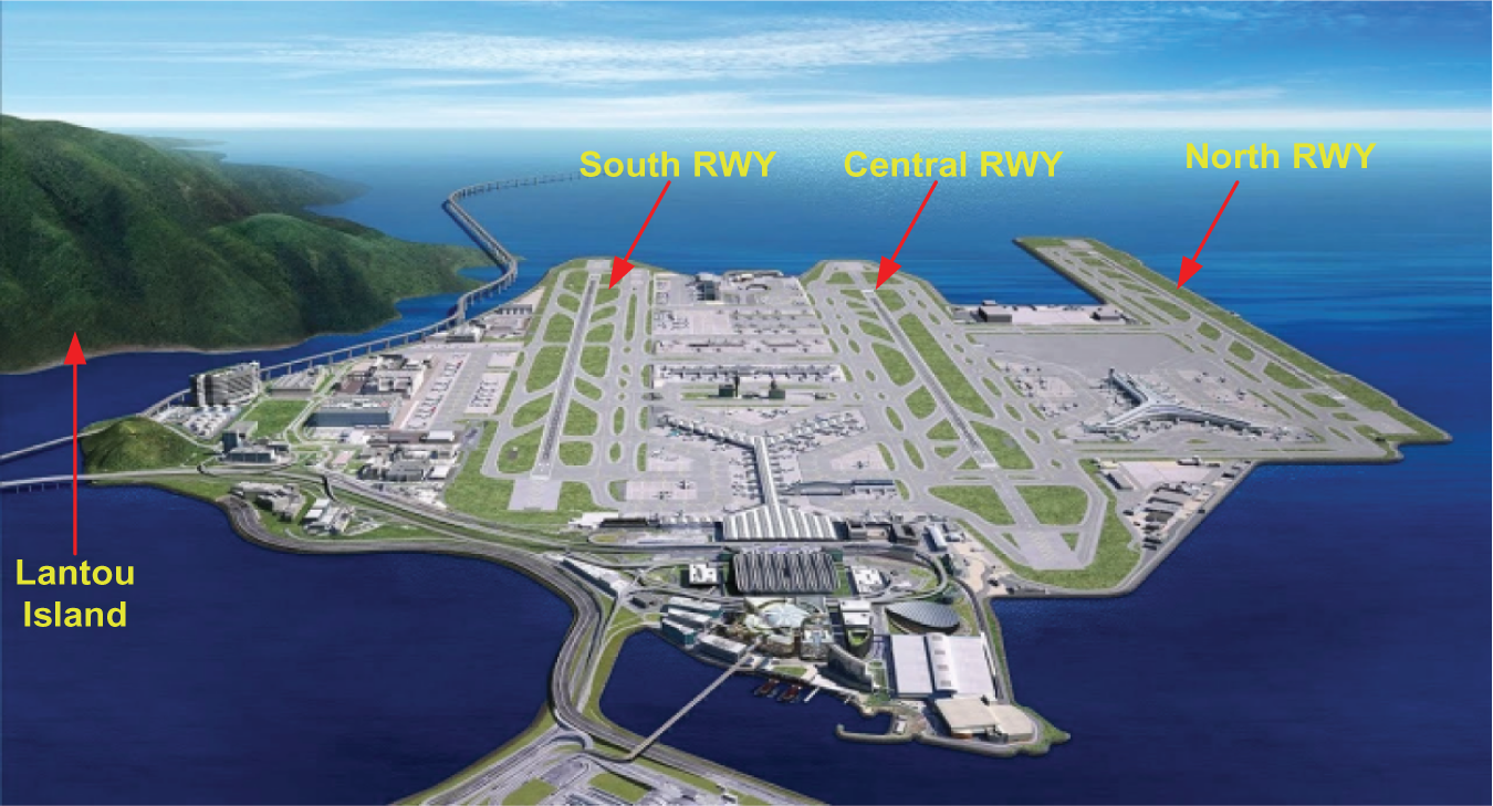
Figure 1: HKIA airport sounding terrain and runway system
HKIA employs two Doppler LiDAR systems to monitor wind conditions and detect WS near runways. These Doppler LiDAR supplied by Mitsubishi Electric are designed to detect WS and turbulence under non-precipitation conditions [42]. These systems rely on a single-frequency pulse laser that captures movements of dust and tiny particulates in the air for precise atmospheric measurements. They are strategically positioned to provide comprehensive coverage of the approach and departure runways of the airport as shown in Fig. 2. One of the Doppler LiDARs is located at the rooftop of a metal platform adjacent to the Midfield Concourse. This LiDAR continuously scans the departure and approach runways focusing on the central and southern runways including 07RA, 25LA, 07RD, and 25LD. Another is the North Runway LiDAR, which is situated near the middle of the new North runway. This LiDAR is dedicated to monitoring the approach and departure paths of northern runway and covers 07LA, 25RA, 07LD, and 25RD. These Doppler LIDAR systems provide detailed insights into critical parameters, which as follows:
• The LiDAR outputs provide precise measurements of headwind gain and loss, enabling the quantification of WS intensity along the glide path of arriving and departing aircraft.
• Each recorded WS event is accurately time-stamped, providing a temporal context that allows for analysis of event frequency, patterns, and seasonal or diurnal variations.
• The systems are configured to measure WS events at various distances along the glide path, providing spatially resolved data relative to the touchdown zone of the runway. This information is crucial for understanding where hazardous wind conditions occur.
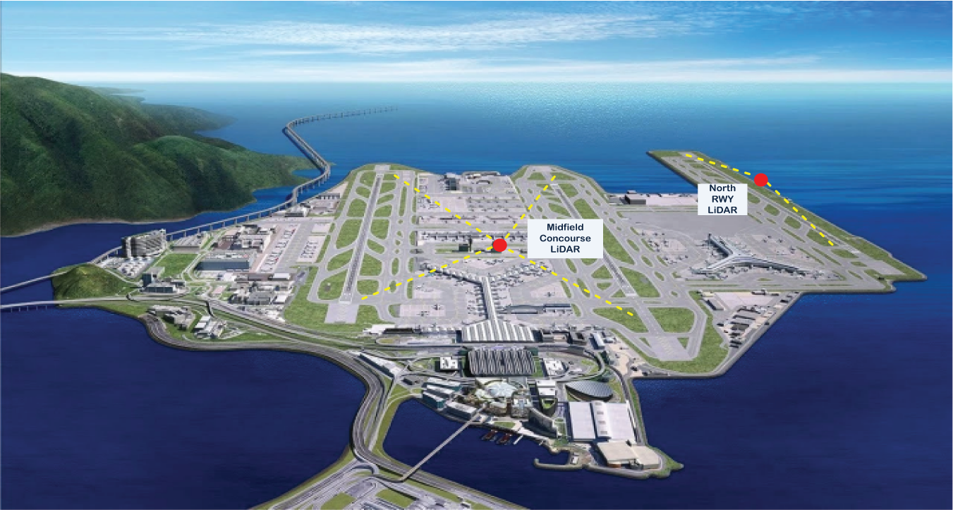
Figure 2: 2 x Doppler LiDAR systems located near northern and central runway of HKIA
3.3 Working Principle of Doppler LiDAR
The Doppler LiDAR system at HKIA operates with an infrared wavelength of approximately 1.5 microns. It has the ability to provide radial resolution of 100 m (range gate) and can compute maximum radial speeds of up to 40 m/s. In clear weather, it can achieve an observation range of 10 to 15 km. However, its performance is notably affected by adverse weather conditions, such as typhoons or heavy rainfall, where the effective range is reduced to under 0.5 km. To enhance its functionality, the system conducts routine plan-position indicator (PPI) scans and is configured for glide path scans along flight paths used during take-off and landing. These glide path scans provide vital insights into the headwind profiles along the runway approaches, enabling precise detection and monitoring of WS conditions. In addition, the laser scanner head of this system is designed for controlled movement in both vertical and azimuthal planes, ensuring comprehensive and precise data acquisition along the glide paths. The glide path scans performed by the two Doppler LiDAR systems at HKIA capture headwind profile data by measuring radial speed. With a revisit interval of approximately one minute, these scans ensure that headwind profiles are updated every minute, providing real time information on wind conditions. This prompt update is critical for detecting WS hazards.
Once the headwind component profiles are generated, the GLYGA algorithm [43] is used to process them. It identifies abrupt changes in headwind profile, known are known as WS ramps and computes a speed increment profile by evaluating the difference between consecutive data points within the headwind profile. Each detected ramp is assigned a severity factor
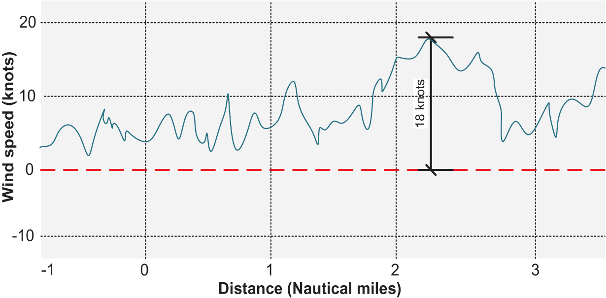
Figure 3: Example of headwind profile showing a peak of 18 knots wind speed
Let the headwind component at a specific location, denoted as
where
Fig. 4 shows an example of Doppler LiDAR observations at HKIA during the night from 24 March to 25 March 2022. The Figure illustrates conical scans in the center with headwind profiles displayed on both sides. A vortex is shown by a red arrow. The middle panels include grey lines extending outward marked at 1, 2 and 3 nautical miles from the runway ends and the corresponding headwind profiles along these lines are shown on either side. The headwind profiles along the glide paths which are straight lines angled at 3° glide path above the horizon leading to the runway where aircraft approach for landing reveal noticeable fluctuations.
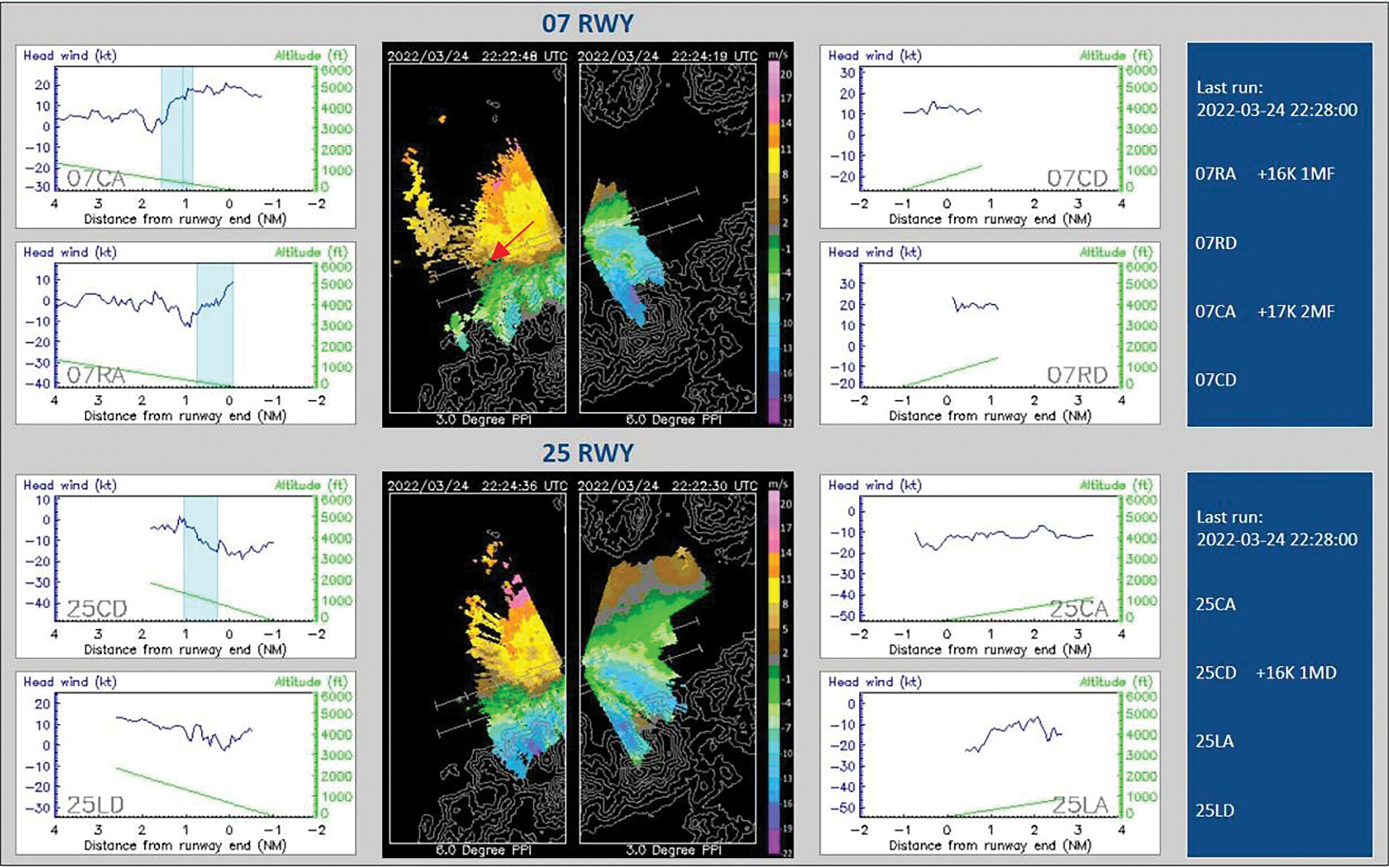
Figure 4: Doppler LiDAR WS observations at HKIA
3.4 Theoretical Overview of Deep Residual Networks (ResNet)
ResNet was developed to overcome the challenges associated with training very deep networks, such as the vanishing gradient problem. As the number of layers increases in a deep neural network, the gradients during back-propagation become extremely small, which makes it difficult to update weights effectively. ResNet addresses this challenge by introducing residual learning through skip connections, which allows the network to learn the residual (difference) between the input and output, instead of directly learning a transformation from input to output. Below is the discussion of different components.
In traditional deep neural networks, each layer learns a mapping
This residual connection (or skip connection) ensures that if the learned residual is close to zero, the network simply outputs the input, preserving the information across layers. Each residual block starts with an input, which in our class is the input data such as assigned runway, WS magnitude and WS encounter from the runway threshold, etc. This input
Here,
where,
This addition allows the network to learn the residual
This completes the forward pass of a residual block, allowing the output
For forward propagation in ResNet, the residual blocks are stacked across multiple layers. The input at each layer undergoes the same process of convolutions, activations, and residual additions, as described. With each forward pass, the model efficiently learns the residual mappings, which help propagate useful information through the network. The deeper architecture (such as ResNet50) is advantageous for capturing more complex relationships in the data that influence the WS intensity. During training, the model optimizes its parameters by minimizing a loss function that quantifies the discrepancy between the predicted and actual WS intensity labels. In binary classification tasks, such as distinguishing between I-WS and NI-WS, the most commonly used loss function is binary cross-entropy [44]. This function is defined as:
where,
In this study, the effectiveness of the different DL and ML classification models for the WS intensity classification is assessed using several key performance metrics, including Precision, Probability of Detection (PoD), F1-score, False Alarm Rate (FAR), Matthews Correlation Coefficient (MCC), G-Mean, and Balanced Accuracy (BA). Precision reflects how accurately the classification model identifies I-WS among all positive classifications. PoD quantifies the ability of model to correctly identify I-WS events relative to all actual occurrences of I-WS. The F1-score provides a balanced evaluation by combining precision and PoD into a single metric, ensuring that both false positives (FP) and false negatives (FN) are considered. FAR measures the proportion of incorrect positive predictions (false alarms) relative to all predicted positive case. MCC is a more comprehensive metric that evaluates the correlation between actual and predicted classifications, taking into account both true and false results, making it particularly useful when dealing with imbalanced datasets. G-Mean captures the balance between sensitivity and specificity, ensuring that the classification model performs well across both positive and negative classes. Finally, BA adjusts for class imbalance by averaging the recall for each class. The mathematical expressions for each metric are shown in Eqs. (10)–(15).
4.1 Details of Model Development
To assess the performance of the our proposed ResNet and other competitive baseline classification models, the data was collected from Doppler LiDAR at HKIA from 2017 to 2021. The data include DATETIME: Timestamp of the WS data captured at specific intervals. RUNWAY: Represents the approaching and departing runways such as 07RA and 25LD. MAGNITUDE: Represents the measured WS intensity in knots, with positive values indicating headwind gain and negative values representing headwind loss. LOCATION: Specifies the exact encounter location of WS from the RWY. Table 1 illustrates the sample data of I-WS event obtained from the Doppler LiDAR of HKIA.

In this research, we have formulated a binary classification problem for WS events. The classification is based on the absolute magnitude of the WS event:
• WS events with a magnitude equal to or greater than 25 knots are designated as I-WS, represented by the class label 1.
• WS events with a magnitude less than 25 knots are designated as NI-WS, represented by the class label 0.
The mathematical expression for this classification can be written as Eq. (16).
This binary classification is crucial for the study as it allows the separation of WS events into intense and non-intense categories for better prediction and mitigation strategies. Prior to training, the SMOTE is applied to balance the training dataset, ensuring that the models are trained on a more balanced representation of I-WS and NI-WS events. In the original training data as shown by pie chart on the left side in Fig. 5, Class 0 (NI-WS) dominates with 97.9% of instances (262,270), while Class 1 (I-WS) accounts for only 2.1% (5517 instances). This significant imbalance can result in biased models that perform poorly when predicting the minority class (I-WS). After applying SMOTE (right pie chart), both classes are perfectly balanced, each representing 50.0% of the dataset with 262,270 instances. By balancing the dataset, SMOTE ensures that DL models can better identify patterns for the minority class (I-WS) and avoid bias toward the majority class (NI-WS). This adjustment enhances the ability of model to accurately detect rare but critical I-WS events, improving prediction reliability.
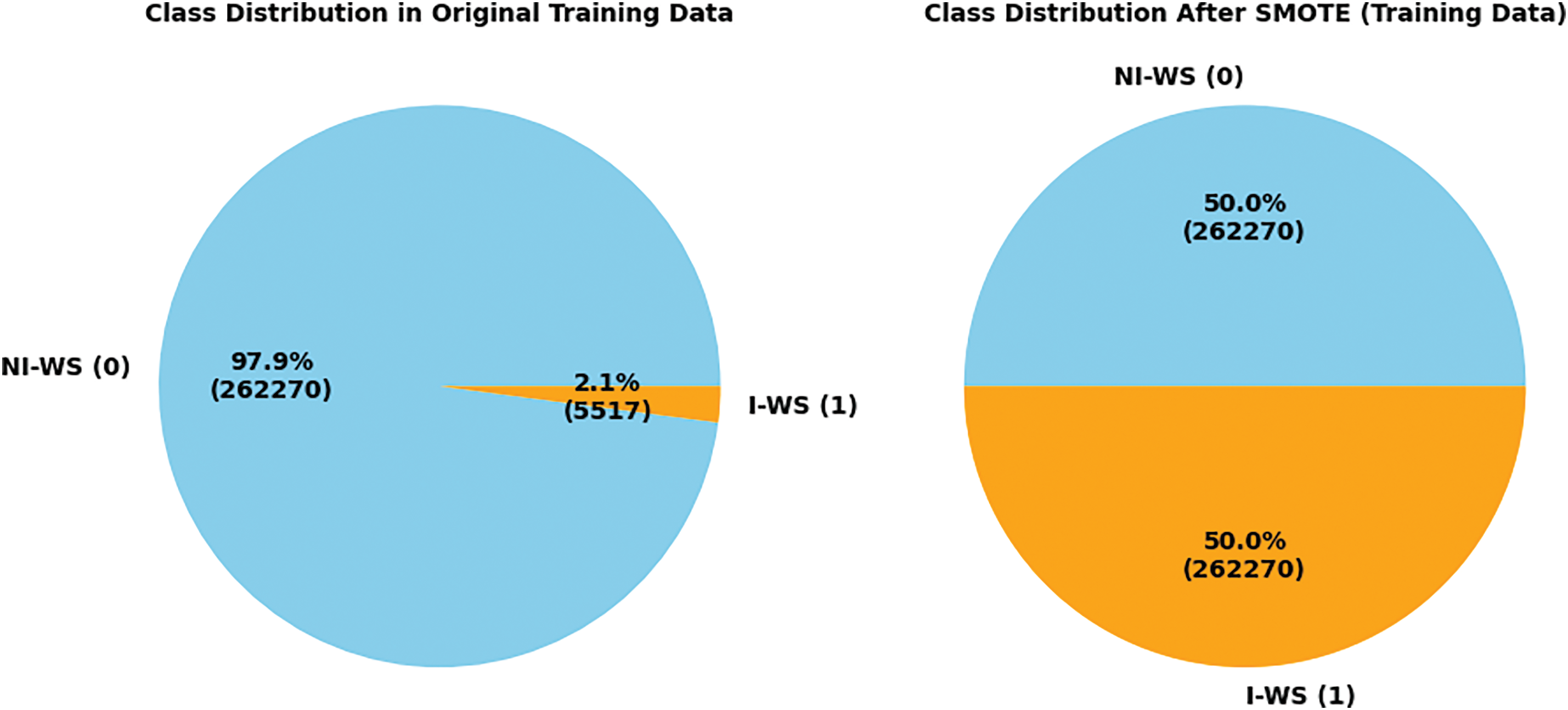
Figure 5: Untreated and SMOTE-treated data of Doppler LiDAR
Following the data preprocessing via SMOTE, two ResNet architectures were utilized for the classification of WS intensity. ResNet34 Architecture involved training a ResNet34 model from scratch using Doppler LiDAR data. The goal was to classify WS intensity effectively by utilizing the ability of model to learn intermediate-level patterns. A ResNet50 model was also trained from scratch, designed to capture more intricate patterns in the data. Its deeper architecture aims to improve classification accuracy by extracting more detailed and complex features. In addition, other DL models including Fully Connected Neural Network (FNN) (Baseline), Convolutional Neural Network (CNN), and Recurrent Neural Network (RNN) and supervised ML models including K-Nearest Neighbors (KNN) and Gene Expression Programming (GEP) were used as baseline models for comparison. In case of DL models, Tables 2 and 3 summarize the different hyperparameters used for these models in the WS intensity classification task. The optimizer plays a critical role in ensuring the stability and effectiveness of the proposed WS intensity classification models. Therefore, Stochastic Gradient Descent (SGD) optimizer is employed for the FNN classifier, while the Adam optimizer is used for the CNN, RNN, and ResNet models. For the ResNet34 model, a learning rate of 0.001 is used. Similarly, a batch size of 200 is selected based on experimental results, which indicate that larger batch sizes contribute to a balance between training accuracy and model convergence. In contrast, for the ResNet50 model, a smaller learning rate of 0.0001 is utilized. This strategy allows the deeper architecture to converge more gradually. This also prevent overfitting while enabling the model to effectively capture the intricate complexities of WS intensity variations.

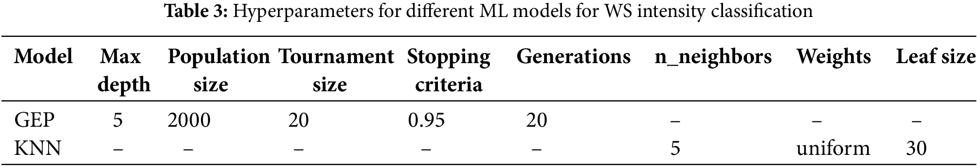
Fig. 6 illustrates the training progress of the ResNet34 and ResNet50 architectures for WS intensity classification, focusing on accuracy and loss function over both the training and testing phases over 50 epochs. Both the training loss (blue line) and validation loss (orange line) decrease steadily during the initial epochs and stabilize after around 15–20 epochs. The gap between training and validation loss is minimal, indicating a good fit of the models without significant overfitting. Both the models demonstrate consistent learning, with both losses converging, illustrating that it is well-trained and generalized effectively.
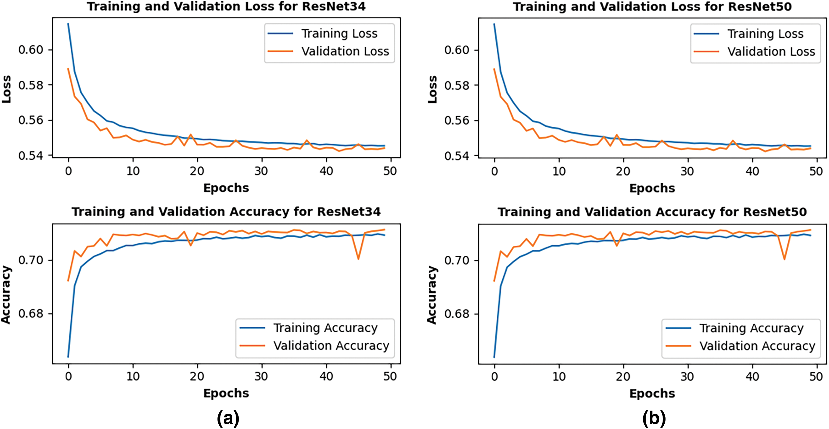
Figure 6: Training progress of ResNet34 and ResNet50 Models for WS intensity classification: (a) Loss vs. Epoch, illustrating the decrease in error over time for both training and testing data, (b) Accuracy vs. Epoch showing the improvement in classification performance as the models converge
The performance of proposed ResNet models and other competitive models in the WS intensity classification task is illustrated using the Confusion Matrix, Receiver Operating Characteristic (ROC) Curve, and Precision-Recall (PR) Curve as shown in Fig. 7. The confusion matrix provides an intuitive understanding of the ability of model to correctly classify both I-WS and NI-WS events by displaying the true positives (TP), false positives (FP), true negatives (TN), and false negatives (FN). Fig. 7a shows the confusion matrix for the ResNet34 model illustrates its performance in classifying NI-WS and I-WS events. The model correctly predicted 66,677 cases of NI-WS (true negatives) and 93,122 cases of I-WS (true positives). However, it misclassified 45,542 NI-WS cases as I-WS (false positives) and 19,463 I-WS cases as NI-WS (false negatives). Fig. 7b shows ROC curve for the ResNet34 model illustrates its performance in distinguishing between NI-WS and I-WS across various classification thresholds. The curve plots the True Positive Rate (TPR or Sensitivity) against the False Positive Rate (FPR) at different thresholds. The orange line represents the performance of ResNet34 performance while the green dashed line is the 45-degree baseline, representing random guessing. The Area Under the Curve (AUC) is 0.78, indicating a reasonably good discriminatory ability of the ResNet34 model to differentiate between the two classes. An AUC of 0.78 shows that the model has a 78% chance of correctly distinguishing between an NI-WS and an I-WS instance. Similarly, the Precision-Recall (PR) curve for the ResNet34 model as shown in Fig. 7c evaluates its performance in distinguishing between NI-WS and I-WS, focusing on the trade-off between precision and recall or PoD at various classification thresholds. The orange line represents the PR curve of the ResNet34 model, while the green dashed line shows the baseline precision, which corresponds to the proportion of positive samples in the dataset. The model achieves an Average Precision (AP) score of 0.74, indicating a moderately good ability to balance precision and recall or PoD across thresholds.
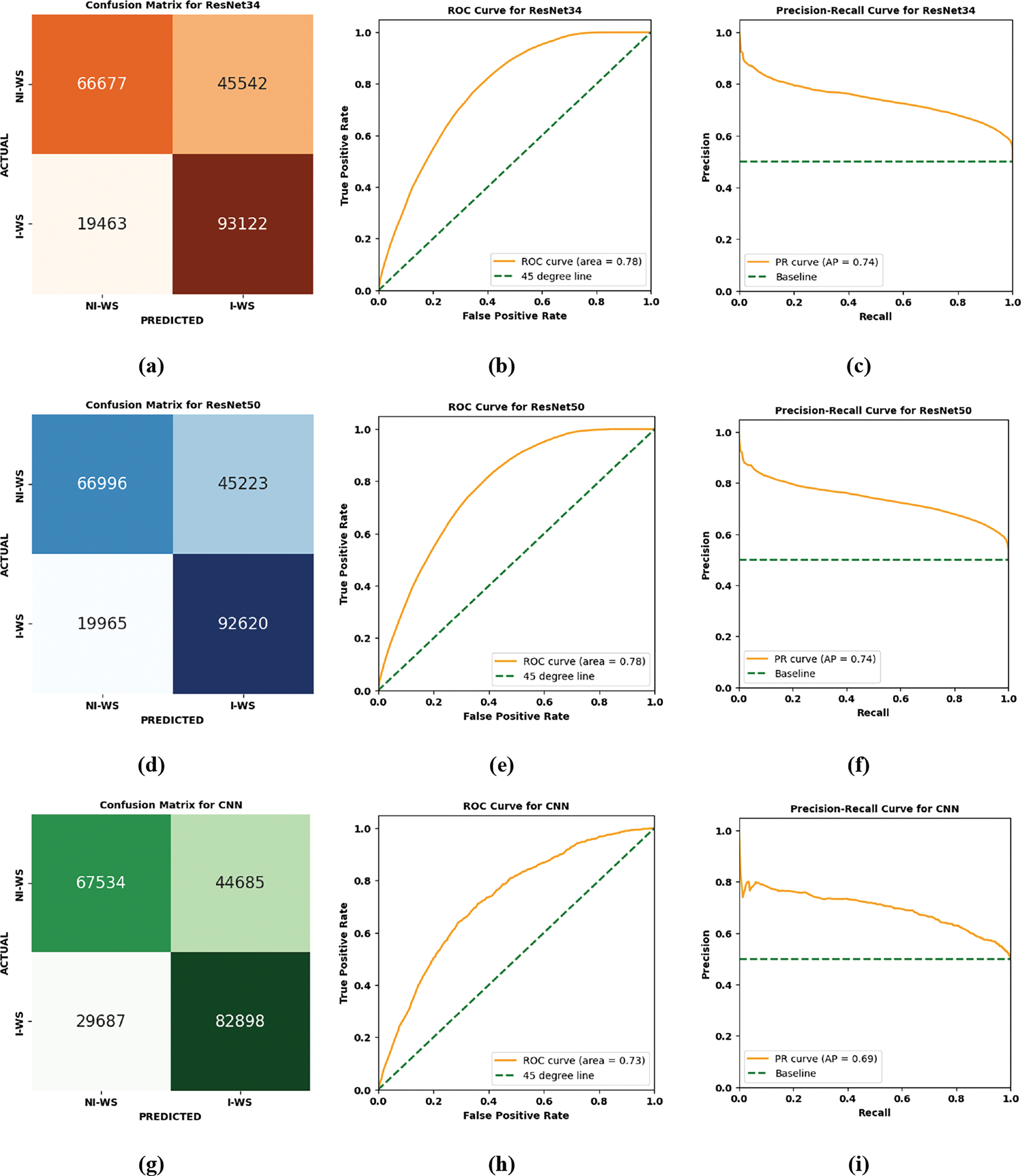
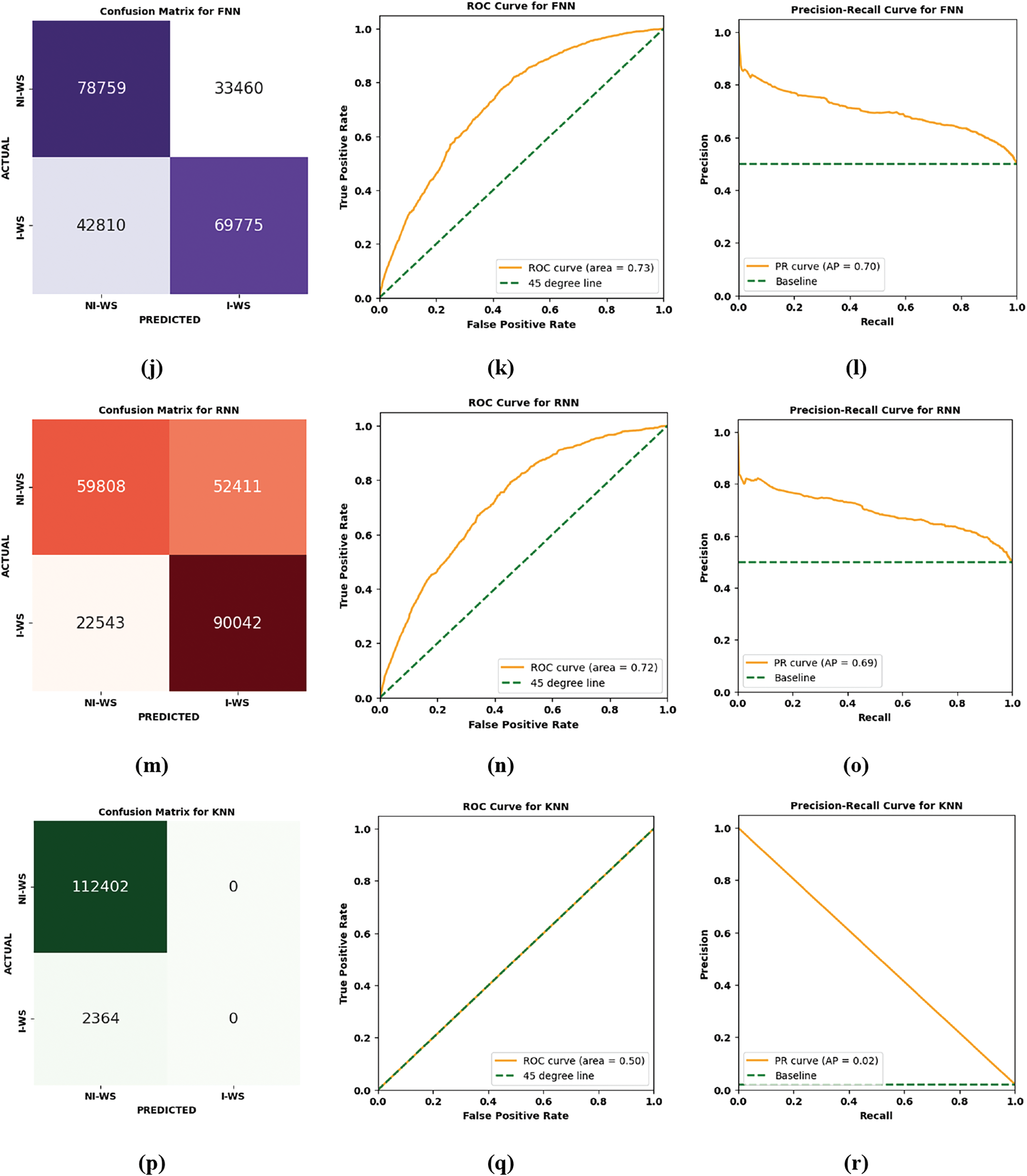

Figure 7: (a) Confusion matrix for ResNet34, (b) ROC curve for ResNet34, (c) Precision-recall curve for ResNet34, (d) Confusion matrix for ResNet50, (e) ROC curve for ResNet50, (f) Precision-recall curve for ResNe50, (g) Confusion matrix for CNN, (h) ROC curve for CNN, (i) Precision-recall curve for CNN, (j) Confusion matrix for FNN, (k) ROC curve for FNN, (l) Precision-recall curve for FNN, (m) Confusion matrix for RNN, (n) ROC curve for RNN, (o) Precision-recall curve for RNN, (p) Confusion matrix for KNN, (q) ROC curve for KNN, (r) Precision-recall curve for KNN, (s) Confusion matrix for GEP, (t) ROC curve for GEP, (u) Precision-recall curve for GEP
The performance of ResNet50 can also be evaluated through its confusion matrix, ROC curve, and Precision-Recall (PR) curve as illustrated in Fig. 7d–f, ResNet50 correctly classified 66,996 NI-WS cases and 92,620 I-WS cases. However, it misclassified 45,223 NI-WS cases as I-WS and 19,965 I-WS cases as NI-WS. Compared to ResNet34, ResNet50 shows a slight increase in I-WS but also a small rise in false negatives, indicating a comparable but slightly varied classification ability. The ROC curve for ResNet50 has an AUC of 0.78, identical to ResNet34. This shows that both models have the same overall ability to discriminate between NI-WS and I-WS. The similarity in AUC indicates that there is no significant improvement in overall classification performance when moving from ResNet34 to ResNet50. ResNet50 achieves an AP score of 0.74, matching the performance of ResNet34. The PR curve for ResNet50 shows similar behavior, with high precision at low recall and a gradual decline in precision as recall increases. This indicates that both models balance precision and recall or PoD to a similar degree.
CNN model correctly classified 67,534 NI-WS cases and 82,898 I-WS cases. However, it misclassified 44,685 NI-WS cases as I-WS (false positives) and 29,687 I-WS cases as NI-WS (false negatives) as shown in Fig. 7g–i. Compared to ResNet34 and ResNet50, CNN has fewer I-WS than ResNet34 and ResNet50, indicating a lower ability to identify I-WS cases accurately. It has higher false negatives (I-WS misclassified as NI-WS), which is critical in safety-related tasks like WS detection. However, CNN has a slightly lower false positive rate compared to ResNet50, showing marginally better specificity. The ROC curve of CNN shows an AUC of 0.73, which is lower than both ResNet34 and ResNet50. This indicates that CNN has weaker overall discriminatory power between NI-WS and I-WS classes. Similarly, the CNN achieves an AP score of 0.69, which is also lower than ResNet34 and ResNet50. This indicates that CNN struggles to maintain a balance between precision and recall or PoD, particularly at higher recall values.
The performance of the FNN model can be assessed using its confusion matrix, ROC curve, and PR curve. The FNN correctly identified 78,759 NI-WS cases and 69,775 I-WS cases as illustrated in Fig. 7j–l. It has misclassified 33,460 NI-WS cases as I-WS and 42,810 I-WS cases as NI-WS. Compared to ResNet34 and ResNet50, FNN demonstrates a higher true negative rate, with fewer NI-WS cases being misclassified as I-WS compared to the ResNet models. However, its true positive rate is lower, as it fails to classify a larger number of I-WS cases correctly, indicated by the higher false negatives. The FNN model achieved an AUC of 0.73, which is slightly lower than the AUC of 0.78 for both ResNet34 and ResNet50. This indicates that FNN has weaker classification between NI-WS and I-WS classes. The PR curve reveals an AP score of 0.70, which is slightly better than CNN (AP = 0.69) but lower than ResNet34 and ResNet50 (AP = 0.74). This shows that FNN maintains a reasonable balance between precision and PoD, although it lags behind the ResNet models in overall effectiveness.
The performance of the RNN can be evaluated using its confusion matrix, ROC curve, and PR curve as shown in Fig. 7m–o. The RNN correctly identified 59,808 NI-WS cases and 90,042 I-WS cases. It misclassified 52,411 NI-WS cases as I-WS and 22,543 I-WS cases as NI-WS. RNN shows improved classification of I-WS cases compared to FNN, with fewer false negatives but it has a higher rate of false positives than ResNet34 and ResNet50, indicating less precision in classification between NI-WS and I-WS. The ROC curve for RNN shows an AUC of 0.72, which is slightly lower than ResNet34 and ResNet50 (AUC = 0.78) but comparable to CNN (AUC = 0.73) and FNN (AUC = 0.73). The ability of RNN to better classify two classes is slightly less effective compared to ResNet models but is similar to that of CNN and FNN. The PR curve indicates an AP score of 0.69, similar to CNN but slightly lower than FNN (AP = 0.70) and ResNet models (AP = 0.74).
In addition, we have also employed ML models including KNN and GEP for the WS intensity classification. As shown in Fig. 7p–r, the KNN model classified 112,402 NI-WS cases correctly but failed to classify any I-WS cases, resulting in 2364 false negatives and 0 true positives. This indicates that KNN has completely failed to classify the I-WS class, classifying all instances as NI-WS. Unlike ResNet34, ResNet50, CNN, FNN, and RNN, which all had varying levels of success in identifying both NI-WS and I-WS, the KNN model fails entirely for I-WS detection. This shows that KNN may not handle the data distribution well in this scenario, particularly for the minority class (I-WS).
The confusion matrix for the GEP model as shown in Fig. 7s–u also reveals its limitations in effectively classifying WS events. The model correctly classified 46,666 instances of NI-WS events, demonstrating moderate success in identifying the majority class. However, it misclassified a substantial 65,736 NI-WS events as I-WS, reflecting a high false positive rate. For the minority class (I-WS), the model managed to correctly identify 1743 cases but failed to recognize 621 I-WS events, which were misclassified as NI-WS. This imbalance suggests that while GEP has some capability to detect critical I-WS events, it struggles to manage the trade-off between sensitivity and specificity, particularly when dealing with the majority class. The ROC curve for the GEP model indicates an AUC of 0.58, which is only slightly better than random guessing (AUC = 0.5). This low AUC value reflects the limited ability of model to discriminate between NI-WS and I-WS events across various thresholds. The PR curve shows an AP score of only 0.02, which is extremely low. This indicates that the GEP model performs poorly in balancing precision and recall, particularly for the minority class (I-WS). The curve shows a rapid decline in precision as recall increases, signifying that the model generates a high number of false positives when attempting to identify I-WS events.
The performance measures presented in Table 4 shows the significant differences in the ability of various DL and ML models to classify WS intensity effectively. Among the models, ResNet34 demonstrates the best overall performance, achieving a balanced accuracy of 0.7106, recall (PoD) of 0.827, and F1-score of 0.7413. These metrics indicate its superior ability to accurately identify I-WS events while maintaining a good balance between sensitivity and specificity. Similarly, ResNet50 performs comparably with only slight decreases in balanced accuracy (0.7098) and F1-score (0.7397), showing the effectiveness of residual learning mechanisms in capturing the complex dynamics of WS events. In contrast, baseline models like CNN, FNN, and RNN show reduced performance, with lower F1-scores (0.6673 for CNN and 0.6466 for FNN) and higher FAR, indicating struggles in achieving a balanced trade-off between false positives and false negatives. RNN slightly outperforms FNN and CNN in recall (PoD) at 0.794 but still lags behind the ResNet architectures in overall classification capability.

On the other hand, the performance of traditional ML models like KNN and GEP is notably inferior. While KNN achieves high precision (0.959) and recall (0.979), its MCC is 0.0000, and its G-Mean is 0.000, reflecting its complete failure to classify I-WS effectively. Similarly, GEP, despite its high precision of 0.9671, suffers from poor recall (0.4318), F1-score (0.5735), and MCC (0.044), showing its inability to balance the classification of both NI-WS and I-WS events. The high FAR (0.2627) for GEP further illustrates its susceptibility to false positives, making it unsuitable for WS intensity classification task.
5 Conclusion and Recommendations
This study utilized Doppler LiDAR data from HKIA to classify WS intensity into I-WS and NI-WS categories using ResNet34 and ResNet50 models, along with comparisons to traditional ML methods including GEP and KNN, and baseline DL models including CNN, FNN, and RNN. Among all models, ResNet34 proved to be the most effective, achieving a balanced accuracy of 0.7106, a recall (PoD) of 0.8271, and an F1-score of 0.7413. This performance highlights its capability to classify rare but critical I-WS events while maintaining a balance between sensitivity and specificity. ResNet50 showed comparable performance, with a balanced accuracy of 0.7098 and an F1-score of 0.7397, establishing itself as the second best model. In contrast, FNN as DL model performed the worst among DL models, with a balanced accuracy of 0.6608, recall of 0.619, and an F1-score of 0.6466, reflecting its limitations in handling imbalanced datasets and capturing WS complexities. Similarly, the KNN model demonstrated poor performance, achieving a balanced accuracy of 0.5000 and a recall of 0.979 for the majority class (NI-WS) while entirely failing to classify the minority class (I-WS). This resulted in an MCC of 0.0000 and a G-Mean of 0.000, reflecting its inability to handle class imbalance effectively. This shows the limitations of KNN in handling Doppler LiDAR data and the complexity of WS dynamics. Given the significant safety implications of WS classification in aviation, different recommendations can be provided:.
• It is recommended that ResNet34 be integrated into airport weather monitoring and safety systems to enhance the detection of hazardous I-WS events. Its reliable performance ensures timely and accurate identification of critical WS events, allowing for proactive measures to ensure aviation safety during takeoffs and landings.
• Future studies could further optimize this framework by incorporating additional meteorological parameters such as temperature, humidity, and wind turbulence, and exploring ensemble techniques to improve generalization.
• Expanding the scope to airports in diverse geographical and meteorological settings would validate the applicability of ResNet34 and effectiveness across different environments.
Despite the promising results, the study has several limitations, which are as follows:
• The use of data from HKIA limits the generalization of the findings to other airports with differing terrain and weather conditions.
• While SMOTE effectively addressed class imbalance in this study, it may not fully replicate the complex relationships inherent in real-world datasets.
• The reliance on Doppler LiDAR data restricts the applicability of the approach in airports without such systems. Future work should focus on overcoming these limitations by integrating multi data sources and developing transferable models to improve the scalability of WS classification frameworks globally.
Acknowledgement: We are thankful to the Hong Kong Observatory of Hong Kong International Airport for providing us LiDAR data as well as grateful to Taif University for their valuable support in this work.
Funding Statement: This research was supported by the National Natural Science Foundation of China (Grant No. 52250410351), the National Foreign Expert Project (Grant No. QN2022133001L), Xiaomi Young Talent Program and Taif University (TU-DSPP-2024-173).
Author Contributions: The authors confirm contribution to the paper as follows: study conception and design: Afaq Khattak, Feng Chen; data collection: Pak-wai Chan; analysis and interpretation of results: Afaq Khattak, Abdulrazak H. Almaliki; draft manuscript preparation: Afaq Khattak and Feng Chen. All authors reviewed the results and approved the final version of the manuscript.
Availability of Data and Materials: The data that support the findings of this study are available from the corresponding author, Afaq Khattak, upon reasonable request.
Ethics Approval: Not applicable.
Conflicts of Interest: The authors declare no conflicts of interest to report regarding the present study.
References
1. Augustin D, Cesar MB. Analysis of wind shear variability and its effects on the flights activities at the Garoua Airport. J Extreme Event. 2022;9(01):2250006. doi:10.1142/S2345737622500063. [Google Scholar] [CrossRef]
2. Yuan J, Su L, Xia H, Li Y, Zhang M, Zhen G, et al. Microburst, windshear, gust front, and vortex detection in mega airport using a single coherent Doppler wind lidar. Remote Sens. 2022;14(7):1626. doi:10.3390/rs14071626. [Google Scholar] [CrossRef]
3. Hon KK, Chan HW. Historical analysis (2001–2019) of low-level wind shear at the Hong Kong International Airport. Meteorol Appl. 2022;29(2):e2063. doi:10.1002/met.2063. [Google Scholar] [CrossRef]
4. Zhang H, Wu S, Wang Q, Liu B, Yin B, Zhai X. Airport low-level wind shear lidar observation at Beijing Capital International Airport. Infr Phy Technol. 2019;96(11):113–22. doi:10.1016/j.infrared.2018.07.033. [Google Scholar] [CrossRef]
5. Boilley A, Mahfouf J-F. Wind shear over the Nice Côte d’Azur airport: case studies. Natural Hazar Earth Syst Sci. 2013;13(9):2223–38. doi:10.5194/nhess-13-2223-2013. [Google Scholar] [CrossRef]
6. Weber M, Cho J, Robinson M, Evans J. Analysis of Operational Alternatives to the Terminal Doppler Weather Radar (TDWR). Project Report ATC-332, MIT Lincoln Laboratory, Lexington, MA, USA; 2007. [Google Scholar]
7. Weber ME. Advances in operational weather radar technology. Lincoln Laborat J. 2006;16(1):9. [Google Scholar]
8. Yoshino K. Low-level wind shear induced by horizontal roll vortices at Narita International Airport. Japan J Meteorol Soc Japan Ser II. 2019;97(2):403–21. doi:10.2151/jmsj.2019-023. [Google Scholar] [CrossRef]
9. Hon K-K. Predicting low-level wind shear using 200-m-resolution NWP at the Hong Kong International Airport. J Appl Meteoro Climatol. 2020;59(2):193–206. doi:10.1175/JAMC-D-19-0186.1. [Google Scholar] [CrossRef]
10. Ryan M, Saputro AH, Sopaheluwakan A. Review of low-level wind shear: detection and prediction. AIP Conf Proc. 2023;2719:020044. doi:10.1063/5.0133460. [Google Scholar] [CrossRef]
11. Chu J, Han Y, Sun D, Han F, Liu H. Statistical interpolation technique based on coherent Doppler lidar for real-time horizontal wind shear observations and forewarning. Opt Eng. 2021;60(4):046102. doi:10.1117/1.OE.60.4.046102. [Google Scholar] [CrossRef]
12. Khattak A, Chan P-W, Chen F, Peng H. Time-series prediction of intense wind shear using machine learning algorithms: a case study of Hong Kong international airport. Atmos. 2023;14(2):268. doi:10.3390/atmos14020268. [Google Scholar] [CrossRef]
13. Coburn J, Arnheim J, Pryor SC. Short-Term forecasting of wind gusts at airports across CONUS using machine learning. Earth Space Sci. 2022;9(12):e2022EA002486. [Google Scholar]
14. Qu J, Zhao T, Ye M, Li J, Liu C. Flight delay prediction using deep convolutional neural network based on fusion of meteorological data. Neural Process Lett. 2020;52(2):1461–84. [Google Scholar]
15. Liu JN, Kwong K, Chan PW. Chaotic oscillatory-based neural network for wind shear and turbulence forecast with LiDAR data. IEEE Transact Syst, Man, Cybernet, Part C (Appl Rev). 2012;42(6):1412–23. [Google Scholar]
16. Khattak A, Chan PW, Chen F, Peng H. Assessing wind field characteristics along the airport runway glide slope: an explainable boosting machine-assisted wind tunnel study. Sci Rep. 2023;13(1):10939. [Google Scholar] [PubMed]
17. Mizuno S, Ohba H, Ito K. Machine learning-based turbulence-risk prediction method for the safe operation of aircrafts. J Big Data. 2022;9(1):29. [Google Scholar]
18. Khattak A, Chan P-W, Chen F, Peng H, Mongina Matara C. Missed approach, a safety-critical go-around procedure in aviation: prediction based on machine learning-ensemble imbalance learning. Adv Meteorol. 2023;2023(1):9119521. [Google Scholar]
19. Dhief I, Wang Z, Liang M, Alam S, Schultz M, Delahaye D. Predicting aircraft landing time in extended-TMA using machine learning methods. In: ICRAT 2020, 9th International Conference for Research in Air Transportation; 2020 Sep; Tampa, FL, USA. [Google Scholar]
20. Schultz M, Reitmann S. Machine learning approach to predict aircraft boarding. Transport Res Part C: Emerg Technol. 2019;98:391–408. [Google Scholar]
21. Dhruv P, Naskar S. Image classification using convolutional neural network (CNN) and recurrent neural network (RNNa review. In: Swain D, Pattnaik P, Gupta P, editors. Machine learning and information processing. Singapore: Springer; 2020. Vol. 1101, p. 367–81. doi:10.1007/978-981-15-1884-3_34. [Google Scholar] [CrossRef]
22. Eskandari H, Imani M, Moghaddam MP. Convolutional and recurrent neural network based model for short-term load forecasting. Elect Power Syst Res. 2021;195:107173. [Google Scholar]
23. Usama M, Ahmad B, Song E, Hossain MS, Alrashoud M, Muhammad G. Attention-based sentiment analysis using convolutional and recurrent neural network. Future Generat Comput Syst. 2020;113:571–8. [Google Scholar]
24. Oruh J, Viriri S, Adegun A. Long short-term memory recurrent neural network for automatic speech recognition. IEEE Access. 2022;10:30069–79. [Google Scholar]
25. Kattenborn T, Leitloff J, Schiefer F, Hinz S. Review on Convolutional Neural Networks (CNN) in vegetation remote sensing. ISPRS J Photogramm Remote Sens. 2021;173(2):24–49. doi:10.1016/j.isprsjprs.2020.12.010. [Google Scholar] [CrossRef]
26. Das S, Tariq A, Santos T, Kantareddy SS, Banerjee I. Recurrent neural networks (RNNsarchitectures, training tricks, and introduction to influential research. Mach Learn Brain Disord. 2023;197:117–38. doi:10.1007/978-1-0716-3195-9. [Google Scholar] [CrossRef]
27. Yang D. Deep learning based image recognition technology for civil engineering applications. Appl Mathe Nonlinear Sci. 2024;9(1). [Google Scholar]
28. Chen J, Wei Z. EEMD-MST-Resnet: a hybrid deep learning approach for predicting passenger flow in urban transportation hubs. Neural Comput Appl. 2024;2018(1):1–21. doi:10.1007/s00521-024-10494-7. [Google Scholar] [CrossRef]
29. Li X, Jiang H, Hu Y, Xiong X. Intelligent fault diagnosis of rotating machinery based on deep recurrent neural network. In: 2018 International Conference on Sensing, Diagnostics, Prognostics, and Control (SDPC); 2018; Xi'an, China: IEEE. p. 67–72. [Google Scholar]
30. Cheng X, Zhang W, Wenzel A, Chen J. Stacked ResNet-LSTM and CORAL model for multi-site air quality prediction. Neural Comput Appl. 2022;34(16):13849–66. doi:10.1007/s00521-022-07175-8. [Google Scholar] [CrossRef]
31. Gao M, Qi D, Mu H, Chen J. A transfer residual neural network based on ResNet-34 for detection of wood knot defects. Forests. 2021;12(2):212. doi:10.3390/f12020212. [Google Scholar] [CrossRef]
32. Almoosawi NM, Khudeyer RS. ResNet-34/DR: a residual convolutional neural network for the diagnosis of diabetic retinopathy. Informatica. 2021;45(7):115–24. [Google Scholar]
33. Wen L, Li X, Gao L. A transfer convolutional neural network for fault diagnosis based on ResNet-50. Neural Comput Appl. 2020;32(10):6111–24. doi:10.1007/s00521-019-04097-w. [Google Scholar] [CrossRef]
34. He K, Zhang X, Ren S, Sun J. Deep residual learning for image recognition. In: Proceedings of the IEEE Conference on Computer Vision and Pattern Recognition; 2016; Las Vegas, NV, USA: IEEE. p. 770–8. doi:10.1109/CVPR.2016.90. [Google Scholar] [CrossRef]
35. Eristi B, Yamacli V, Eristi H. A novel microgrid islanding classification algorithm based on combining hybrid feature extraction approach with deep ResNet model. Electr Eng. 2024;106(1):145–64. doi:10.1007/s00202-023-01977-2. [Google Scholar] [CrossRef]
36. Desanamukula VS, Teja TD, Rajitha P. An in-depth exploration of ResNet-50 and transfer learning in plant disease diagnosis. In: 2024 International Conference on Inventive Computation Technologies (ICICT); 2024; Lalitpur, Nepal: IEEE. p. 614–21. [Google Scholar]
37. Chawla NV, Bowyer KW, Hall LO, Kegelmeyer WP. SMOTE: synthetic minority over-sampling technique. J Artif Intell Res. 2002;16:321–57. doi:10.1613/jair.953. [Google Scholar] [CrossRef]
38. Shun C. Ongoing research in Hong Kong has led to improved wind shear and turbulence alerts. ICAO J. 2003;58(2):4–6. [Google Scholar]
39. Carruthers D, Ellis A, Hunt J, Chan P. Modelling of wind shear downwind of mountain ridges at Hong Kong International Airport. Meteorol Appl. 2014;21(1):94–104. doi:10.1002/met.1350. [Google Scholar] [CrossRef]
40. Lau S. Windshear and turbulence detection and warning at Hong Kong International Airport. In: 13th Newsletter of the Working Group on Training, the Environment and New Developments (TREND); 2001; Hong Kong: Commission for Aeronautical Meteorology, WMO. [Google Scholar]
41. Chan P, Shun C, Kuo M. Latest developments of windshear alerting services at the Hong Kong International Airport. In: 14th Conference on Aviation, Range, and Aerospace Meteorology; 2010; Atlanta, GA, USA. [Google Scholar]
42. Corporation ME. Mitsubishi electric to supply terminal doppler lidars in Hong Kong; 2015 [cited 2024 Nov 15]. https://www.proceedings.com/content/074/074902webtoc.pdf [Google Scholar]
43. Chan P, Shun C, Wu K. Operational LIDAR-based system for automatic windshear alerting at the Hong Kong International Airport. In: 12th Conference on Aviation, Range, and Aerospace Meteorology; 2006. [Google Scholar]
44. Das R, Chaudhuri S. “On the separability of classes with the cross-entropy loss function.” arXiv: 190906930. 2019. [Google Scholar]
Cite This Article
 Copyright © 2025 The Author(s). Published by Tech Science Press.
This work is licensed under a Creative Commons Attribution 4.0 International License , which permits unrestricted use, distribution, and reproduction in any medium, provided the original work is properly cited.
 Downloads
 Citation Tools