Adaptive Time Synchronization in Time Sensitive-Wireless Sensor Networks Based on Stochastic Gradient Algorithms Framework

1  Introduction

Wireless sensor networks (WSNs) are distributed control systems utilized for a variety of sensing and instrumentation applications. A precise, adaptable, and reliable time synchronization protocol for WSNs is required due to a number of reasons, such as the close connection between sensors and the physical environment [1], the lack of power for stationed nodes, the requirement for large-scale deployment, decentralized topologies, and unpredictable and intermittent connectivity between network nodes [2,3]. Large WSNs need sophisticated time synchronization techniques, especially if the network experiences dynamic changes from time to time and communication among WSN nodes is unstable, resulting in packet losses.

Time delays between node clocks which are caused by transmission and reception, media access, channel propagation, interrupt management, encoding and decoding, and byte alignment, all contribute to synchronization issues between WSN nodes. Therefore, several time synchronization protocols have been implemented as discussed in the literature [4–8]. The protocols can be divided into two variants based on the network architectures adopted in the synchronization. They include centralized protocols (CPs) and distributed protocols (DPs). The centralized and structured algorithms can be further divided into tree-structured and cluster-structured protocols. CPs often accomplish global network synchronization in time by synchronizing all network nodes to a leader node in a hierarchical tree structure or by utilizing network clusters. In most CPs, this leader node gets elected after the preceding one fails. In DPs, nodes communicate clock parameters in their neighborhoods and agree on a global time via trees, clusters, or a leader node. The following section examines various relevant and current centralized and distributed time synchronization techniques.

1.1 Review of Centralized Protocols

The Flooding Time Synchronization Protocol (FTSP) [9] is an ad hoc and multi-hop time synchronization strategy. This protocol assumes the base node as the node with the lowest identity value; the rest of the nodes use its clock value as their reference time. The synchronization packets are transmitted regularly by the root node to all network nodes, containing their local time. FTSP uses linear regression to adjust for drifts between nodes and reference nodes. However, the main issue with this approach is that the resynchronization time is relatively short, requiring a high overhead and as a huge bandwidth during each resynchronization phase, resulting in a significant energy cost.

Chen et al. [10] proposed a closed-loop feedback-based synchronization protocol that implements a proportional-integral (PI) controller to compensate for clock drift. The accuracy of this method is determined by the output and transient times. This technique requires a base node and is synchronized via a tree, hence it is susceptible to connection and node malfunctions.

Yildirim et al. [11] demonstrated that the synchronization accuracy and scalability of WSNs are significantly reduced by the slower flooding transmission speed used in FTSP. In addition, they observed the fact that the PulseSync protocol’s speedy flooding has several disadvantages [12]. They created a procedure that eliminates the negative aspects of delayed flooding in FTSP without changing the flood’s propagation rate. Through tests, they demonstrate that the synchronization accuracy and slow-flooding scaling could be significantly improved using the proposed clock speed agreement technique.

FloodPISync and PulsePISync time synchronization algorithms were introduced in [13] to improve the PulseSync protocol. The techniques represent and change node clocks as a PI controller. The algorithms’ calculations, simulations, and experimental investigations efficiently synchronizes the nodes. Using FloodPISync, the PI analogy changes the nodes clock drift and offset to improve the synchronization of all nodes to the reference node. A similar concept is applied for PulsePISync with the quick flooding technique adapted based on the PulseSync protocol.

Lee et al. [14] presented a novel time synchronization technique that uses a dual-clock delayed message mechanism. The clock synchronization system uses the flooding time-sync approach with one-way timing messages to ensure low power consumption for WSN nodes. The maximum-likelihood technique for time parameters is then employed to calculate the time parameters, such as clock drift and offset. However, because the flooding strategy necessitates transmitting many packets in order to accomplish synchronization, it is inefficient for extensive networks.

1.2 Review of Distributed Protocols

Apicharttrisorn et al. [15] introduced an energy-efficient gradient protocol which is efficient in terms of power and diffused. The technique implements progressive mean estimation and drift prediction to achieve temporal convergence and slope. Because the protocol broadcasts continuously, it produces small trends that use much energy from WSNs. Each node computes the continuous averaging of clock values immediately after it receives the broadcast packet from one of its neighbors. The global time increases as the stepwise averaging is decreased.

Schenato et al. [16] introduced the Average Time Sync (ATS) consensus algorithm. The mechanism works by averaging the nodes’ local times in order to achieve global synchronization in the network. In addition, two consensus approaches are cascaded to compute the clock properties as the clock convergence to a specific value.

Consensus Clock Synchronization (CCS) [17] employs the average consensus technique to compute and adjust each node’s clock offset. The drifted values of each node’s clock from the global consensus time is calculated by accumulating clock offset errors. The drifted values of each node’s clock from the global consensus time are calculated by accumulating clock offset errors. The errors are removed in each iteration from the offset compensation. The clock drift is adjusted by using those data. This system, such as the ATS, is entirely distributed, although it converges somewhat slowly.

Cheng et al. [18] proposed the Maximum Time Synchronization (MTS) protocol which is aimed to maximize local time for global synchronization. Compared to previous methods, this approach has a faster convergence speed. The technique adjusts the skew or offset clock values by defining a finite value. The protocol is entirely distributed, asynchronous, and resilient to node failure. The approach is also feasible for replacing or adding additional nodes. The same study suggested another approach, the Weighted Maximum Time Synchronization Protocol, which addresses the delay issue related to receipt and broadcast packets.

Wu et al. [19] introduced a clustered consensus time synchronization (CCTS) protocol for synchronizing nodes’ clocks in WSNs. The method is distributed in operation and relies on consensus. This CCTS technique was classed as intracluster or intercluster time synchronization. The simulation findings revealed that the node’s communication traffic is reduced. However, the node could be subjected to failures due to dynamic topologies which is caused by the leader nodes.

Yildirim et al. [13] introduced Proportional Integral Synchronization (PISync), a distributed time synchronization technique based on a proportional-integral (PI) controller. They introduced the AvgPISync protocol, an average consensus-based and completely distributed PISync protocol based on the PISync algorithm, and conducted real-world tests and simulations to assess its performance. They reported that the AvgPISync protocol has some advantages compared to current techniques because it possesses a minimal code footprint, requires minimal data to be exchanged, has not much overhead associated with memory allocation and CPU, stores no unique time information, and has highly scalable steady-state condition and global clock error.

A technique to synchronize poor infrastructure sensor networks in severe environments was proposed in the literature [20,21]. The studies presented three novel asynchronous, decentralized, and energy-efficient time synchronization techniques that only require a single hop of sparse communication with unlabeled network nodes to determine the time of the gateway node. The time of a node in a discrete system can be observed as a changing factor whose growth is either inhibited or initiated asynchronously by a different dynamic switching process. The protocols are designated as Unidirectional Asynchronous Flooding (UAF), Bidirectional Asynchronous Flooding (UAF), and Timed Sequential Asynchronous Update (TSAU). After substantial modeling, the protocols are developed and tested on the MICAz sensor node platform. The energy usage of the suggested protocols, memory needs, convergence time, and local and global synchronization flaws are evaluated compared to Flooding Time Synchronization Protocol (FTSP) and FloodPISync. The findings suggested that the procedures outperform the well-known methods.

An Energy Efficiency Time Synchronization Protocol (EETS) for WSNs was presented in the literature [22]. This protocol was demonstrated to take advantage of the pairing of the Auto Regressive Moving Average (ARMA) model and the Kalman filter model in time series prediction, which can both address the shortcomings of the Kalman filter prediction and the low prediction accuracy of ARMA in complex environments. The validation results demonstrate energy efficiency for WSNs and validate the effectiveness of EETS, which was done by the authors using a prototype system. However, this protocol was not evaluated against existing protocols for real-time performance using parameters such as memory usage, synchronization precision, and convergence time.

In a newer study, the unique synchronization technique proposed in the literature [23] takes advantage of both the CP and DP architectures. The hybrid time synchronization protocol (HTSP) technique uses a temporary reference node to drastically shorten convergence times, while an average-based consensus is used in regular operations to handle node failures. The protocol is distributed, but each node is programmed to switch between the reference and consensus modes while in operation. Despite performing better than specific established protocols such as FTSP and GTSP, this protocol exhibited greater global synchronization error values. In addition, more real-time experimental work is required to verify enhanced synchronization accuracy and convergence time claims.

Abdul-Rashid et al. [24] presented a new time synchronization protocol for wireless sensor networks (WSNs). The authors addressed the challenges of achieving accurate synchronization in unstructured multi-hop networks by formulating the problem as an optimization task. They utilized the Butterfly Optimization Algorithm (BOA) to optimize clock parameters and achieve global synchronization across the network. The proposed protocol was experimentally evaluated against two existing protocols: the Newton Inspired Time Synchronization protocol and the Average Proportional Integral Synchronization protocol. Results indicated that the new protocol significantly outperformed these alternatives in terms of synchronization accuracy. The study highlighted the effectiveness of BOA in enhancing time synchronization in WSNs and suggested potential directions for future research in this area.

Recently, numerous attempts have been made to improve the convergence rate and synchronization error. The studies [25–27] utilized the concept of Packet-Coupled Oscillators (PkCOs). The Minimum Variance Time Synchronization (MVTS) algorithm in the literature [24] uses output feedback to reduce the noise on the accumulation of synchronization errors. Static feedback control using H∞ design solution is utilized to adjust the clock drift, which works well in the 21-node network using a 32.768 MHz clock rate as implemented in [27]. Both solutions adopted the Linear Matrix Inequality optimization framework for the proposed synchronization algorithms. However, the PkCOs approach was criticized in [3] as the performance degrades when adopted at a lower clock rate, which is widely used in most existing industrial applications.

1.3 Distributed and Centralized Protocols

In general, DPs have a steady state value and are resilient and adaptable to changes in the network topology. They are also impacted by network propagation delays and noise, just as other protocols. Since surrounding nodes can communicate with one another to reach the consensus point based solely on the initial analysis, the protocols are distinguished by low-complexity repetitive procedures, eliminating the requirement to transfer information to a reference node. Conversely, CPs are typically simple to set up and consist mainly of pairwise synchronization followed by global network synchronization. The protocols do, however, have a number of shortcomings, including the substantial overhead associated with building the entire tree structure, which makes them unsuitable for use in networks with dynamic topologies and typically adds extra time and overhead. At the same time, another node is connected to the network, or a reference election is necessary.

1.4 Contribution

In the literature [13], the protocol uses two dynamic control parameters called proportional and integral gains, α and β, to update clock parameters that present stability issues in the synchronization. These parameters are assumed to be constant in the formulation of the synchronization problem in [28], but actually, they must be updated as well prior to the update of clock parameters. The convergence of the control parameters was also shown to depend on the network topology. In [29], the clock rate update is done using only GraDes, which is known to have some disadvantages such as sensitivity to initial parameters, differentiable cost function, local minima traps, and over-fitting. The proposed framework can trade off between WSN applications, requirements, and the advantages of different stochastic algorithms for time synchronization.

In more recent approaches like EETS [22], using Kalman Filters and the ARMA model will render the synchronization protocol ineffective in real-world WSN applications. Although Kalman filtering offers precise state estimation and noise reduction capabilities, its computational demands, sensitivity to model inaccuracies, scalability challenges, and implementation costs make it less suitable for clock synchronization. Simpler and more energy-efficient synchronization algorithms, such as gradient-based or distributed consensus algorithms, can be better alternatives for highly constrained or large-scale WSNs [30]. Also, the HTSP protocol [23] is expected to have a significant overhead due to the combined operations of the much older protocols of FTSP and Gradient Time Synchronization Protocol (GTSP), and hence its adaptivity to changes in network dynamics remains to be proven.

The proposed synchronization framework improves the methods in [28,29] with a more general and optimized approach. The proposed framework can trade off between WSN application requirements and the advantages of different stochastic algorithms for time synchronization.

This study outlines the following contribution:

1.    A novel adaptive framework is proposed for WSN time synchronization that uses the advantages of different stochastic gradient algorithms for clock frequency adjustments.

2.    Generalized conditions are derived for which any stochastic gradient-based synchronization algorithm will converge and closed-form asymptotic variance for synchronization precision comparisons between different stochastic gradient algorithms.

3.    Design and implement a light-weight multi-hop time synchronization protocol based on the suggested framework.

4.    Evaluate the proposed protocol using several stochastic gradient algorithms through real-time experiments and compare performances against AvgPISync.

The remainder of the paper is structured as follows: Section 2 covers the system concept; Section 3 presents the proposed clock synchronization architecture; Section 4 describes the convergence analysis of the proposed synchronization strategy; Section 5 explains the analytical performance of different stochastic gradient algorithms based on the suggested framework; Section 6 presents the experimental comparative evaluation of the synchronization protocols. Lastly, Section 7 concludes the paper.

2  System Model

Ordinary nodes dispersed throughout a comparatively small region or sensor field regularly send readings to a base or gateway node in a sparsely distributed WSN. Most base nodes possess many resources, in contrast with ordinary nodes with smaller power, communication rate, and memory. In addition, the gateway node in many WSNs is connected to a reliable and precise time reference, like a GPS receiver. For clarity in the presentation of the proposed framework, this study provides a glossary of terms and symbols used in Appendix A to improve readability and accessibility.

Fig. 1 indicates that all the other sensor nodes synchronize with the hardware clock of the gateway node τG in the absence of exterior time input. In this model, nodes i and j are 1-hop neighbors of the gateway node, G, and periodically receive clock values from the gateway, G, and exchange clock values with their 1-hop neighbors. After a set period of packet exchanges, each node uses a chosen stochastic gradient algorithm to update its clock value using the current clock value and received neighborhood clock values. This process will update the clock value to the latest update time, tk, at the communication instant, k, which updates to the next logical clock, c(tk), in the neighborhood, as discussed further in Section 2.3. Global network synchronization is then expected within accepted error margins after several clock update rounds.

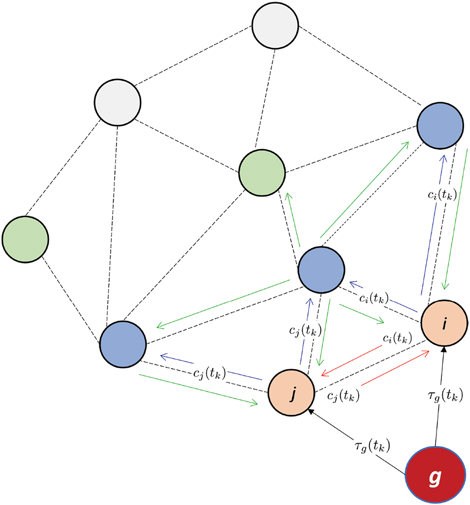
Figure 1: Time synchronization network concept in which nodes share neighboring clock data to synchronize their clocks to that of a gateway node, τG

2.1 Network Model

A WSN with symmetric connections is assumed, which can be depicted as an undirected graph 𝒢=(𝒱,ℰ). The sensor nodes in the network are represented as the set of vertices, 𝒱={vi|i=1,2,…,N}, where N=|𝒱| denotes the number of vertices in 𝒱, and the operational network links between the nodes are represented as an edge set, ℰ, such that (vi,vj)∈ℰ if nodes i and j can exchange information. Nodes that directly communicate with node i are known as the neighboring nodes of i and can be denoted by the set 𝒩i={vj|ℰi,j∈ℰ}.

2.2 Clock Model

In a Wireless Sensor Network (WSN), each node is furnished with a hardware clock, denoted as τ, which is constructed using a crystal oscillator. As the nominal frequencies of the oscillators can vary due to factors like temperature fluctuations and aging, the hardware clocks experience drifts. Following the definition of a hardware clock provided in [21], the hardware clock τi of any given WSN node i at a time t>t0 is characterized by an initial clock value τi(t0) and the oscillator frequency f(ζ)∈[f^−fmax,f^+fmax].

τi(t)=τi(t0)+∫t0tf(ζ)dζ(1)

where fmin and fmax are the oscillator’s fundamental frequency’s lowest and greater bounds, f^, and the clock’s drifting behaviors are represented as follows:

f(t)=f^+r(t)(2)

where r(t)∼U(−fmax,fmax) [13].

2.3 Generalized Update of Clock Parameters

Because the clock parameters of a physical clock are incapable of being modified, every network node additionally retains a logical clock parameter that is a function of the present physical clock value, τi(t), and a logical clock rate, δ(t). The representation of this logical clock c(t) is

c(t)=c(t0)+Δ(t)[τ(t)−τ(t0)](3)

Using the distributed network architecture shown in Fig. 1 as a basis, we may express this update rule as follows [31]: at a transmission moment, k and the most recent update time, tk a node, i∈𝒱 changes its subsequent logical clock as

ci(tk+)=ci(tk)+Δi(tk+)[τi(tk+)−τi(tk)](4)

As for the logical clock speed, Δi(tk)=ddtk[ci(tk)], whether it gradually slows or accelerates depends on its present value which is an estimate of the relative frequency f^fi(t). The clocks of the WSN nodes can be kept synchronized utilizing this progressing model by recursively updating the logical clock of node i using every update of the offset value, ci(tk), and the clock rate, Δi(tk). The adjustment of Δi is accomplished using an adaptive approach, as seen in Fig. 2, to establish a resilient synchronization model. Eq. (4) can be expressed as follows:

c¯i(tk)=Δi(tk+)τ¯i(tk)(5)

where c¯i(tk)=ci(tk+)−ci(tk) and τ¯i(tk)=τi(tk+)−τi(tk).

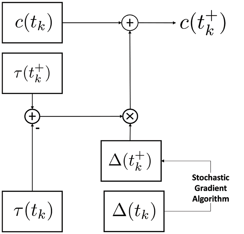
Figure 2: Suggested clock setup for node synchronization

Considering that M<N=|𝒱| nodes modify their clocks at tk, a shortened version of (5) can be expressed as follows, abusing notation a little bit, say k=tk for convenience.

C(tk)=Δ¯(tk)T(tk)(6)

where T(tk)=[τ¯1(tk),…,τ¯M(tk)], C(tk)=[c¯1(tk),…,c¯M(tk)] and Δ¯(tk)=[Δ1(tk),…,ΔM(tk)].

3  Proposed Framework for Clock Synchronization

In the proposed framework, Since the gateway clock, τG(tk) ((7)), is presumed to be precisely ticking at every point in time k, every node must attempt to monitor and predict it. The above synchronization challenge can be thought of as an estimation problem.

τG(tk)=k×1f^=tk(7)

where B is the resynchronization period of nodes. A linear dynamic update strategy may be derived from this mechanism, using a training set {x(tk),d(tk)}≡{T(tk),τ^g(tk)} for the WSN’s update and global synchronization. Fig. 3 illustrates this generalization. For the dynamic update of clock variables in this framework, we employ the deviation, ei(tk), between each node’s logical clock and the gateway clock, as stated in (8).

ei(tk)=c¯i(tk)−τG(tk)(8)

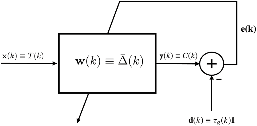
Figure 3: Model framework for clock synchronization for the sake of illustration k is used for tk in the model

Thus, an apparent comparability is found between the synchronization problem and the adaptive filter in Fig. 3. This comparability is shown by

d(tk)≡τG(tk)1; w(tk)≡Δ¯(tk); x(tk)≡T(tk); y(tk)≡C(tk)(9)

where 1=[1,1,…,1]T. This abstraction matters because it allows the clock’s speed to be modified using any stochastic gradient technique. The evolving logical clock has to be updated by first updating the clock rate using a stochastic gradient algorithm to carry out clock synchronization, as shown in Fig. 2. Given a desired output, τ^g(tk), the problem of synchronization could be described as estimating τ^g(tk) from τ^i(tk) so as to minimize the cost function. Assuming we define the square of the neighborhood error defined in (8) as a cost function given by

J(Δi)=e2(Δi(tk))(10)

The goal of the synchronization algorithm is to achieve in each pooling cycle, an optimal clock rate Δi⋆ corresponding to, Jmin.

Δi⋆=argminΔi⁡J(Δi(tk))(11)

The update of Δi should be such that J(Δi(tk))<J(Δi(tk+1)). Hence, a stochastic gradient algorithm can be emplyed to search for the optimal clock rate, Δi⋆ over several iterations using a step size, μ. To perform the clock rate update based on the model in Fig. 3, this study adopts a generic form of stochastic gradient algorithms, with update equations having a linear or non-linear function of the logical clock input, T(tk) represented as follows:

Δ¯(tk+1)=Δ¯(tk)−μg[T(tk)]e(tk)(12)

where g[.] is some positive function of the input, i.e., g[.]>0 and μ∈R is the step size. The generic equation given in (12) can be used to represent different algorithms such as the least mean square (LMS) algorithm, the Newton search algorithm, the GraDes algorithm, the normalized-LMS (N-LMS) algorithm and the simplified form of LMS named Sign-Regressor LMS or Sign-Data LMS which can all be used for the update of the logical clock rate. The derivation of g[τ¯i(tk)] for each algorithm is given in Appendix B and summarized in Table 1.

4  Convergence and Steady State Analysis

The piece-wise form of the clock rate update in (12) can be written for some node i as follows:

Δi(tk+1)=Δi(tk)−μg[τ¯i(tk)]ei(tk)(13)

Considering that there is a delay in transmission and node i is inside the communication distance of the gateway node, G, or {G|ℰi,g∈ℰ} of β between i and G, the synchronization error at i with respect to G at packet reception time tk=Δk, can be computed using

ei(tk)=ci(tk)−τg(tk)=ci(tk)−tk−βk(14)

Then node i updates its logical clock value with the error offset given by

ci(tk+1)=ci(tk)−ei(tk)=tk+βk.(15)

At the second packet reception time tk+1 following this correction, the synchronization error ei(tk) will primarily be caused by the different hardware clock frequency of node i. Hence the error function given in (8) can be generalized as

ei(tk)=ci(tk)−kB−βk=Δi(tk+)τ¯i(tk+)−kB−βk(16)

Lemma 4.1. βk is modeled as a zero-mean Gaussian distributed random variable with variance by applying the central limit theorem, σβ2 [21].

4.1 Asymptotic Convergence and Steady-State in the Mean Sense

For simplicity, we assume ei(tk)=ei(tk) and Δi(tk)=Δi(tk). We then define e(tk+1) and Δi(tk+1) based on the update Eqs. (15) and (16) as follows:

e(tk+1)=Δi(tk)τ¯i(tk)−(B+βk+1−βk)(17)

Δi(tk+1)=Δi(tk)−μg[τ¯i(tk)][Δi(tk)τ¯i(tk)−(B+βk+1−βk)]

Δi(tk+1)=Δi(tk)[1−μg[τ¯i(tk)]τ¯i(tk)]−μg[τ¯i(tk)](B+βk+1−βk)](18)

Combining (17) and (18) into a state representation yields (19).

[e(tk+1)Δi(tk+1)]=[0τ¯i(tk)01−μg[τ¯i(tk)]τ¯i(tk)][ei(tk)Δi(tk)]+(B+βk+1−βk)[−1μg[τ¯i(tk)]](19)

Definition 4.1 (ℒp Convergence). A sequence of ℱ-measurable random variables x(n):n∈N is said to converge to an ℱ-measurable random variable x in ℒp sense if

limn→∞E[|x(n)−x|p]=0

Theorem 4.1. The update of the logical clock rate of a node i∈𝒱,(i,G)∈ℰ using a stochastic gradient algorithm of the form (13) will converge in the ℒp sense to an asymptotically stable point if and only if the step size μ is chosen in the range, (0,2P1), i.e., μ must be chosen based on the inequality

0<μ<2P1(20)

where p=1, P1=E[g[τ¯i(tk)]τ¯i(tk)] and E[.] denotes an expectation operation.

Proof of Theorem 4.1. To assess the pairwise convergence of the proposed generalized algorithm for clock synchronization in the mean-sense, we evaluate ℒp, p=1 convergence of (19) by taking the expectation of (19).

[E[e(tk+1)]E[Δi(tk+1)]]=[0Bf^01−μE[g[τ¯i(tk)]τ¯i(tk)]][E[ei(tk)]E[Δi(tk)]]+[−BμBE[g[τ¯i(tk)]]](21)

For the technique to asymptotically converge in the mean-sense, a unit circle must contain the modes λ1,λ2 of E[Φ(tk)]=Φ¯(tk). It finds the eigenvalues as [λ1,λ2]=[0,(1−μE[g[τ¯i(tk)]τ¯i(tk)])] according to the premise |λI−Φ¯(tk)|=0. Consequently, 0<μ<2E[g[τ¯i(tk)]τ¯i(tk)] is a necessary and sufficient condition for asymptotic convergence in the mean-sense.   ∎

Based on Theorem 4.1, our proposed system can converge to an asymptotically stable points of error and rate define as

[limk→∞E[ei(tk)]limk→∞E[Δi(tk)]]=[e(∞)Δi(∞)](22)

Theorem 4.2. The evolving pairwise synchronization error, ei and the clock rate, Δi for node i synchronizing to the clock of a perfectly ticking gateway node, G converge to the steady state values ei(∞)=B(Bf^×P2−1) and Δi(∞)=B×P2, respectively, where P2=E[g[τ¯i(tk)]]E[g[τ¯i(tk)]τ¯i(tk)].

Proof of Theorem 4.2. To assess the pairwise convergence of the proposed framework for clock synchronization in terms of the synchronization error and the clock rate, we utilize (17) and (18). Each algorithm used for the rate update aims to converge to a rate that achieves a zero synchronization error.

From (17), it can write the steady state error as follows:

ei(∞)=Bf^Δi^(∞)−B,(23)

and the asymptotic clock rate is given by

Δi(∞)=(1−μE[g[τ¯i(tk)]τ¯i(tk)])Δi(∞)+μBE[g[τ¯i(tk)]]

After some simple manipulations, then

Δi(∞)=BE[g[τ¯i(tk)]]E[g[τ¯i(tk)]τ¯i(tk)](24)

Substituting (24) in (23) yields a steady-state error of

ei(∞)=B(Bf^×E[g[τ¯i(tk)]]E[g[τ¯i(tk)]τ¯i(tk)]−1)(25)

and let E[g[τ¯i(tk)]]E[g[τ¯i(tk)]τ¯i(tk)]=P2. Since the communication rate,B and the nominal oscillator frequency, f^ will always be positive and non-zero, i.e., B>0,f^>0 it is obvious from (25) that a necessary and sufficient condition for zero asymptotic synchronization error is for P2=1Bf^.    ∎

Lemma 4.2. Consider a WSN whose nodes carry out time synchronization based on the model presented in Figs. 2, 3, and using a stochastic gradient algorithm of the form given by (13) for clock rate update. Time Synchronization will eventually be achieved with zero steady-state error, e(∞)=0 and nominal ticking rate, Δi(∞)=1f^ if and only if, P2=1Bf^.

The steady-error asymptotic variance must be as small as possible to maintain tight global synchronization among network nodes [32]. For any particular stochastic gradient algorithm, the value of μ must be chosen to satisfy Theorem 4.1 and be as small as possible. Hence, to further analyze the convergence behavior of this proposed paradigm for synchronization, the asymptotic variance of the synchronization error is given by Theorem 4.3.

Theorem 4.3. The asymptotic variance in synchronization error of a stochastic gradient algorithm of the form given by (13) for clock rate update is given by

Var[e(∞)]=μ2(B2+Bfmax22f^2)(Q3+(B2+σD2)f^2Q1−3Bf^Q32μQ2+2μ2Q3)+Bfmax2f^2+σD2(26)

where Q1=E[g2[τ¯i(tk)]], Q2=E[g[τ¯i(tk)]τ¯i(tk)], and Q3=E[g2[τ¯i(tk)]τ¯i2(tk)].

The proof of Theorem 4.3 is given in Appendix C. From the analysis of our generalized paradigm for clock synchronization, we observe that the steady-state values and the conditions are all independent of the propagation error.

Lemma 4.3. A node i synchronizing in a network with gateway node will eventually achieve zero steady-state error, ei(∞)=0 with variance var[ei(∞)] and nominal ticking rate, Δi(∞)=1f^, once Theorems 1 and 2 are satisfied, irrespective of the statistics of the propagation delay of transmission between the node and the gateway or neighboring nodes.

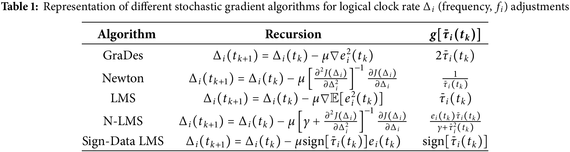
5  Theoretical Performance of Stochastic-Gradient Algorithms

In this section, we extend the analysis of the proposed generalized paradigm for synchronization to study the convergence and steady state of node clock rate or frequency adjustment using the LMS algorithm, the Newton search algorithm, the GraDes algorithm, N-LMS algorithm, Sign-Error LMS and Sign-Data LMS. The following steps can be taken to undertake this analysis while choosing a particular stochastic gradient algorithm for clock rate update, the following steps can be taken:

1.    Reconfigure the chosen stochastic gradient algorithm to fit the form of (13) and estimate a simplified form of the function g[τi(tk)].

2.    To obtain the range of values for which the clock frequency update will converge in the mean sense, find P1 and substitute it into (20).

3.    To obtain the steady state values of the synchronization error, e(∞) and the clock rate, Δi(∞) in the mean sense, find P2 and substitute it in the equations in Theorem 4.2.

4.    Calculate and simplify Q1,Q2 and Q3 using g[τi(tk)] and substitute it into (26) to obtain the asymptotic variance.

5.1 Gradient Descent (GraDes) Algorithm Inspired Time Synchronization

In the literature [28], the GraDes based time synchronization protocol is expressed as follows:

ci(tk+1)=ci(tk)+ei(tk)=tk+βk, and(27)

Δi(tk+1)=Δi(tk)−2μτ¯i(tk)ei(tk)(28)

Therefore g[τi(tk)]=2τ¯i(tk). From this configuration, we obtain the variable for convergence in the mean sense as

P1=2E[g2(τ¯i(tk))]=2B2f^2(1+fmax23Bf^2)

For this algorithm to converge, μ must be chosen to be based on the inequality of

0<μ<1B2f^2(1+fmax23Bf^2)(29)

This condition is more accurate as compared to that presented in [28] which approximates ∂e(Δi)∂Δi=2ei(tk)τ¯i(tk)=2ei(tk)E[τ¯i(tk)]. Furthermore, after some simple manipulations the variable P2 is calculated as P2=12Bf^(1+fmax23Bf^2), and therefore substituting P2 into Theorem 4.2, gives e(∞)=B(12(1+fmax3Bf^2)−1) and Δi(∞)=1f^(2(1+fmax23Bf^2)).

For the asymptotic variance, we compute Q1 and Q2 and for g[τi(tk)]=τ¯i(tk) as follows:

Q1=4E[τ¯i2(tk)]=4(B2f^2+Bfmax23)

Q2=2E[τ¯i2(tk)]=2(B2f^2+Bfmax23)

The lower-bound approximation is adopted for Q3 using Jensen’s inequality where

Q3=4E[τ¯i4(tk)]≥4E4[τ¯i(tk)]=4B4f^4

Inserting these values in (26) and simplifying yields,

Var[e(∞)]=μ(B2+Bfmax22f^)(B4f^4+f^2(B2+σD2)(B2f^2+Bfmax23)−3B5f^5B2f^2+Bfmax23−2μB4f^4)+Bfmax2f2+σD2.(30)

Lemma 5.1. The asymptotic error and clock rate for the GraDes algorithm used for clock rate update in synchronization for WSNs will reach zero steady-state, e(∞)=0, nominal ticking rate, Δi(∞)=1f^, and have a convergence condition of μ∈(0,2B2f^2) if and only if:

3Bf^2=−2fmax2(31)

5.2 Least Mean Square (LMS) Algorithm Inspired Time Synchronization

The instantaneous LMS algorithm can be adopted for the update of logical clock rate and hence, the update of clock parameters for this algorithm can be given as follows:

ci(tk+1)=tk+βk, and(32)

Δi(tk+1)=Δi(tk)−μei(tk)τ¯i(tk)(33)

Hence, g[τi(tk)]=τ¯i(tk). From this configuration, similar to the GraDes-based algorithm, it obtains the variable for convergence in the mean sense as

P1=2E[g2(τ¯i(tk))]=B2f^2(1+fmax23Bf^2)

For this algorithm to converge, μ must be chosen to based on the inequality

0<μ<2B2f^2(1+fmax23Bf^2)(34)

In addition, after some simple manipulations the variable P2 is calculated as P2=1Bf^(1+fmax3Bf^2), and therefore substituting P2 into Theorem 4.2, e(∞)=B(1(1+fmax23Bf^2)−1) and Δi(∞)=1f^(1(1+fmax23Bf^2)). We compute Q1, Q2 and Q3 for g[τi(tk)]=τ¯i(tk) as follows:

Q1=Q2=E[τ¯i2(tk)]=B2f^2+Bfmax23

and

Q3=E[τ¯i4(tk)]≥E4[τ¯i(tk)]=B4f^4

Inserting these values in (26) and simplifying yields,

Var[e(∞)]=μ2(B2+Bfmax22f^)(B4f^4+f^2(B2+σD2)(B2f^2+Bfmax23)−3B5f^5B2f^2+Bfmax23−μB4f^4)+Bfmax2f2+σD2.(35)

Lemma 5.2. The asymptotic error and clock rate for the LMS algorithm used for clock rate update in time Synchronization for WSNs will eventually reach zero steady-state, e(∞)=0 and nominal ticking rate, and Δi(∞)=1f^, and have a convergence condition of μ∈(0,2B2f^2) if and only if:

3Bf^2⋙fmax2 or B⋙fmax23f^2(36)

Proof of Lemma 5.2. Given P1=B2f^2(1+fmax23Bf^2) and P2=1Bf^(1+fmax3Bf^2), if the fraction, fmax23Bf^2⟶0 then P1=B2f^2 and P2=1Bf^.

Since the clock frequency cannot be zero, fmax23Bf^2≈0 only if, the numerator fmax2 far exceeds 3Bf^2. Now assuming f^=ρfmax, 0<ρ<1, then fmax23Bf^2=13ρ2B. Since fmax is fixed for a sensor node oscillator, 13ρ2B⟶0 if the beacon rate, B is really high.    ∎

5.3 N-LMS and Newton Algorithm Based Time Synchronization

The equations of the time synchronization protocol inspired by the Newton algorithm are given by

ci(tk+1)=ci(tk)+ei(tk)=tk+βk, and(37)

Δi(tk+1)=Δi(tk)−μei(tk)τ¯i(tk)(38)

The clock rate update in (38) is reminiscent of the N-LMS algorithm for a scalar parameter which can be given as follows:

Δi(tk+1)=Δi(tk)−μei(tk)τ¯i(tk)γ+τ¯i2(tk)

Assuming an infinitesimal γ, and comparing to (13), g[τi(tk)]=1τ¯i(tk). Hence, P1=1. Therefore for this algorithm to converge, μ must be chosen to based on the inequality

0<μ<2(39)

The variable P2 is also calculated to be P2=1Bf^, and therefore from Theorem 4.2, e(∞)=0 and Δi(∞)=1f^. This result is also consistent with that presented in [29]. To calculate the asymptotic variance, Q1, Q2 and Q3 are computed from Theorem 4.3. Substituting g[τi(tk)]=1τ¯i(tk) in their respective equations and simplifying,

Q1=E[τ¯i−2(tk)]≈E−1[τ¯i2(tk)]=1B2f^2+Bfmax23

Q2=Q3=1

Inserting these values in (26) and simplifying yields,

Var[e(∞)]=(B2+Bfmax22f^)(μ2fmax+2μf^2σD22−4μ−2μ2Bf^2+2μ2fmax2)+Bfmax2f2+σD2.(40)

5.4 Sign-Data LMS Algorithm Inspired Time Synchronization

The Sign-Error LMS algorithm is a modified variant of the conventional LMS algorithm and can also be used to update the logical clock rate. In this algorithm, Instead of using τ¯i(tk), this algorithm uses its sign. This leads to the following recursions for clock parameters:

ci(tk+1)=ci(tk)+ei(tk)=tk+βk, and(41)

Δi(tk+1)=Δi(tk)−μsign[τ¯i(tk)]ei(tk)(42)

sign[τ¯i(tk)]={−1if τ¯i(tk)<00if τ¯i(tk)=01if τ¯i(tk)>0

Since the the hardware clock is constantly ticking, we assume τ¯i(tk)=τi(tk+)−τi(tk)≠0 or −1 and hence g[τi(tk)]=sign[τ¯i(tk)]=1

From this formulation, P1=E[sign[τ¯i(tk)]τ¯i(tk)]=Bf^. Therefore for this algorithm to converge, μ must be chosen to based on the inequality

0<μ<2Bf^(43)

In addition, the variable P2 is calculated to be P2=1Bf^, and therefore from Theorem 4.2, e(∞)=0 and Δi(∞)=1f^. We compute Q1, Q2 and Q3 for g[τi(tk)]=1 as follows:

Q1=1

Q2=E[τ¯i(tk)]=Bf^

Q3=E[τ¯i2(tk)]=B2f^2+Bfmax23

Inserting in (26) and simplifying yields,

Var[e(∞)]=μ2(B2+Bfmax22f^)(f^2(B2+σD2)+(1−Bf^)(B2f^2+Bfmax23)B2f^2+Bf^+Bfmax23)+Bfmax2f2+σD2.(44)

5.5 Theoretical Comparison of Synchronization Algorithms

This section summarizes the theoretical differences and similarities between the LMS algorithm, the Newton search algorithm, the GraDes algorithm, the SignData-LMS algorithm, and the N-LMS algorithm for synchronization clock rate update. The yardstick for this exercise is based on the steady-state synchronization error and clock rate, the convergence time, the asymptotic error variance, and the order of algorithm complexity.

5.5.1 Steady-State Convergence

Using the steady-state values of synchronization error and the clock rate, three algorithms: the N-LMS, the Newton search, and the Sign-Data LMS are observed to converge to zero synchronization error and the nominal clock rate, 1/f^. This means that the algorithms will eventually evolve to a steady state independent of network size N and beacon period B. However, the steady-state conditions of the GraDes and LMS algorithms depend on the maximum frequency of the node clock oscillator, fmax, the beacon rate, B, and the nominal oscillator frequency, f^. However, the convergence of the LMS algorithm is better than that of the GraDes algorithm because if the conditions in Lemmas 5.1 and 5.2 are satisfied, the LMS algorithm converges to 1/f^, whereas the GraDes algorithm converges to 2/f^. Furthermore, we compare the conditions of convergence of the algorithms. All algorithms’lower bound of the step size, μ, is zero. However,except for the Newton and N-LMS algorithms having upper bounds of μ to be 2, the upper bound of μ for all the other algorithms is inversely proportional to Bf^. Table 2 compares the convergence and steady-state performance of all algorithms used for node logical clock updates.

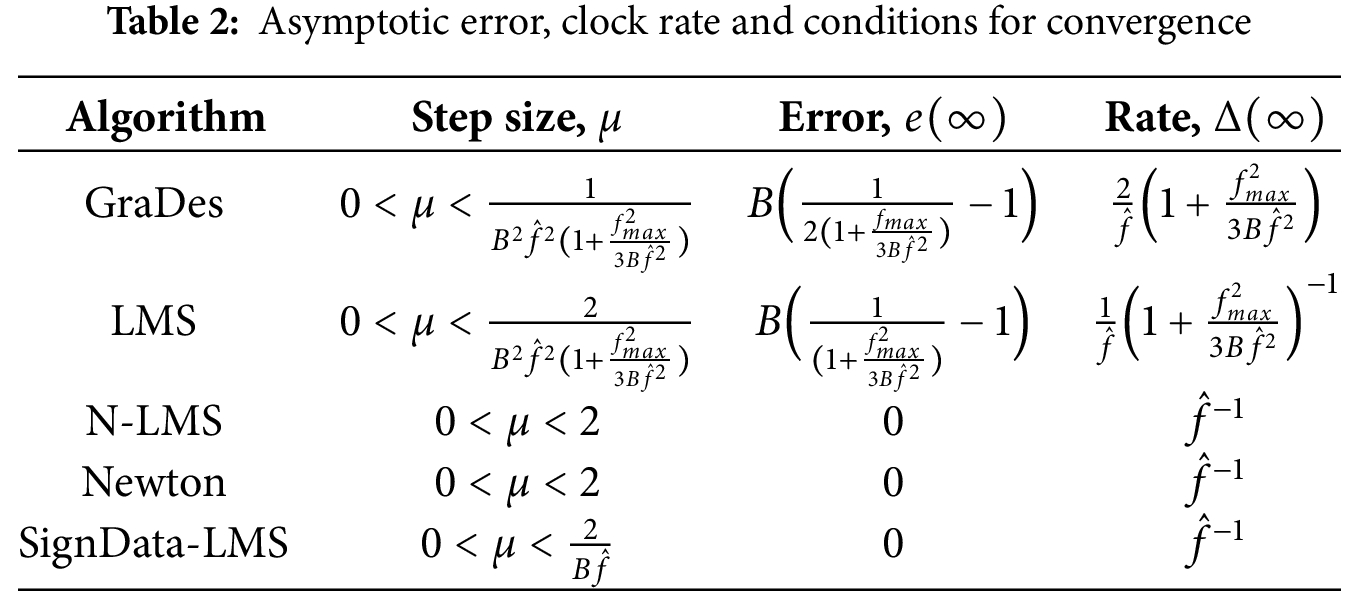
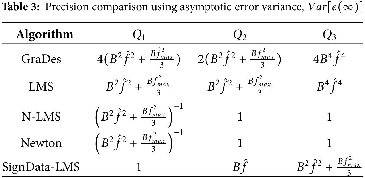
5.5.2 Asymptotic Error Variance

The asymptotic variance indicates the statistical distance between the steady-state synchronization error of each network node and the global average steady-state error. The degree of synchronization precision of a protocol, which is inversely proportional to the asymptotic variance, can be compared between protocols. From the generalized derived closed-form asymptotic variance of all protocols, we observe that the differences in each protocol’s variance lie in the third multiplicative factor,which we denote here as ψ and given as

ψ=−Q3(3Bf^−1)+(B2+σD2)f^2Q12μQ2+2μ2Q3(45)

It can be observed from (45) that the asymptotic variance, Var[e(∞)], is minimized if Q1 is minimum and, Q2 and Q3 are maximum. Comparison of the parameters for the five clock rate update algorithms is given by Table 3. Based on this criteria for synchronization comparison, it is clear that SignData-LMS outperforms all other algorithms since it has a minimum Q1 and a maximum Q2 and Q3. In comparison, the N-LMS and Newton algorithms have lower values of Q1 but the values of Q2 and Q3 are infinitesimal as compared to those of SignData-LMS. However, since all the parameters are minimal for the N-LMS and Newton algorithms, this will result in lower values of Var[e(∞)] compared to the LMS and GraDes algorithms. In addition, Q1, Q2, and Q3 for LMS are all less than those of GraDes, and since Q2 and Q3 for GraDes are far higher than those of LMS, we conclude that the GraDes algorithm will outperform the LMS algorithm in terms of synchronization precision. This indicates that, theoretically, the most precise algorithm for clock synchronization precision is the SignData-LMS, followed by the N-LMS and Newton algorithms, then the GraDes algorithm. The LMS-based synchronization algorithm performs poorly in terms of synchronization precision.

5.5.3 Complexity

The complexity of all the stochastic gradient-based algorithms, i.e., GraDes, LMS, N-LMS, Newton, and SignData-LMS, are similar. In the algorithms, for each node i, the update of clock parameters is carried out every synchronization round or beacon rate, B. Hence, the algorithm will run in multiples of B until convergence is attained. Hence, the overall complexity is 𝒪(B). However, with each B, node i updates its logical clock every Ts using received logical clock values from its Ni neighbors. Hence, all algorithms’computation complexity is 𝒪(BTsNi).

5.6 Multi-Hop Synchronization with Generalized Protocol

Based on the pair-wise synchronization assessment, this section describes an extensive procedure for achieving time synchronization in WSNs. A generic protocol is devised that allows any node to achieve local synchronization and by extension, allows network-wide synchronization. The gateway node, G, and its associated timestamp, τG, may only be directly accessible to a small number of nodes; hence, a decentralized averaging procedure is utilized to synchronize all nodes with G. The clock rate, Δ, is updated using the stochastic adaptive search method, which modifies the logical clock speed every synchronization cycle. The protocol assumes an underlying MAC protocol is assumed by the protocol. Algorithm 1 presents the pseudo-code for the protocol implementation of node i. Upon activation, node i sets several variables to zero, such as ci, which represents the estimated clock value, Δi, which represents the oscillator frequency and two auxiliary variables, ClockError and Received, which are utilized for decentralized averaging (Line 3).

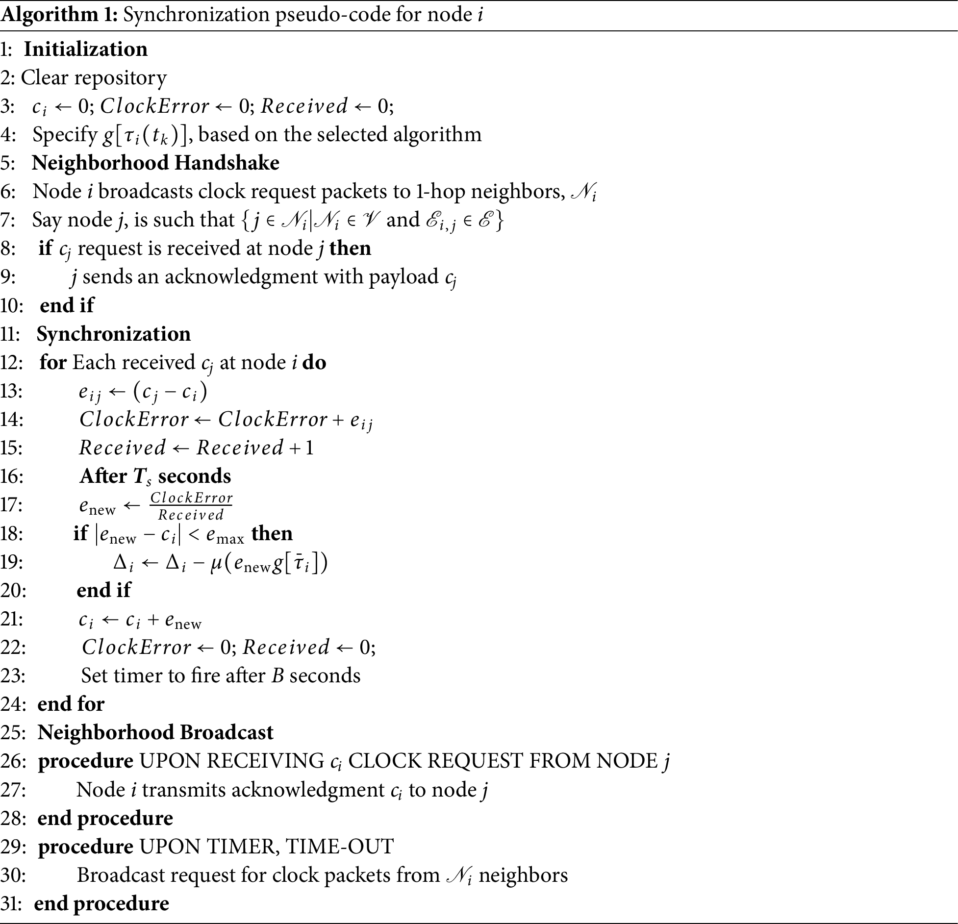
After clearing its stored data and determining g[τi(tk)] according to the selected algorithm, node i broadcasts a request to its neighbors for their clock values (Line 4). Following receipt of this request, node j, a neighbor of i, sends i an acknowledgment packet that includes cj, its clock value (Lines 5–7). Node i computes the difference between its current time value, ci, and the received time value, cj, for each received acknowledgment with a clock value, cj. It then accumulates this value in the ClockError variable for all neighboring time values. In addition, each reception increases by one in the Received variable (Lines 8 to 11). Node i waits for a duration, Ts⋘B1 (Line 13).

The node updates of Δi is done using the computed update criterion if the absolute value of enew is less than a pre-calculated maximum error, emax. This value is given by emax=2Bf^−1fmax [13] based on the frequency difference between the two arbitrary nodes captured at a specific window size B. The emax reflects the trade-off between synchronization precision and the expected frequency deviation under typical operational conditions, considering hardware variability and environmental noise. Then, node i sets a timer to go off in B seconds (Lines 16 to 18), updates the clock value, ci, resets the auxiliary parameters, and, when the timer goes off, node i broadcasts request packets for local clock values. Last but not least, node i sends an acknowledgment to j with its most recent clock whenever it receives a clock request from node j nearby.

6  Experimental Results and Discussion

This study implemented the proposed generalized protocol configured with five (5) stochastic algorithms, GraDes, LMS, N-LMS, Newton, SignData-LMS and also AvgPISync [13] for a MICAz WSN platform using TinyOS operating system. Based on our evaluation of recent protocols, even though there are newer alternatives, AvgPISync stands out as a high-performing adaptive and distributed protocol with proven practical implementation results. Therefore, it is an excellent candidate for comparison with newly developed protocols.

6.1 Experimental Test-Bed

The experimental test-bed utilizes MICAz nodes from Memsic, which are built around a 7.37 MHz 8-bit Atmel Atmega128L microcontroller. The nodes are equipped with 4 kB of RAM, 128 kB of program flash, and a Chipcon CC2420 radio chip, capable of transmitting data at a rate of 250 kbps at a frequency of 2.4 GHz. The 7.37 MHz quartz oscillator on the MICAz board serves as the clock source for the timer used for timing measurements. Since the timer operates at one-eighth of the oscillator frequency, each timer tick occurs approximately every 921 kHz (approximately 1 μs), resulting in f^ equal to 1 MHz.

TinyOS-2.1.2, installed on the Ubuntu Linux Distribution, is used as the base operating system for all experimental work. The MICAz board’s CC2420 transceiver timestamps synchronization packets at the MAC layer using the timing measurement timer [21]. Although the motes are a bit old-fashioned, they have the same architecture as most of the recent motes and are still used by several contemporary researchers [33–35] for WSN protocol design. Also, the proposed adaptive algorithms are hardware-neutral, as they primarily target algorithmic convergence and synchronization precision and are expected to perform better on more recent devices. Additionally, the higher clock rates and lower energy consumption in contemporary devices could further enhance the performance of our framework.

The test-bed layout used for our experiments is based on a grid and line topology of 16 nodes, as shown in Fig. 4, with a diameter of 8 between nodes. The grid topology allows us to evaluate the performances of protocols on a dense network, and the line topology is employed to study protocol performances on a sparse network and the effects of the shape of networks on synchronization accuracy and convergence. Each testbed is configured such that one node acts as the gateway node and the others as ordinary nodes, which are programmed independently with the synchronization protocol. A specialized node configured to act as the base station or sink is connected to a PC and gathers all time-sync packets onto a computer for analysis. In our experiments, a beacon period B of 30 s was used for all protocols. The experimental parameters for AvgPISync, β, αmax, and emax are kept respectively at 1, 3.33×10−8 [13], and for N-LMS, γ=1×10−6. The same step size of μ=0.1 is used in all protocols to ensure objective assessment of all protocols. At the start of each experiment, the network nodes are powered on in a random sequence within a 45-s window, and each experiment runs for a duration of approximately 330 min.

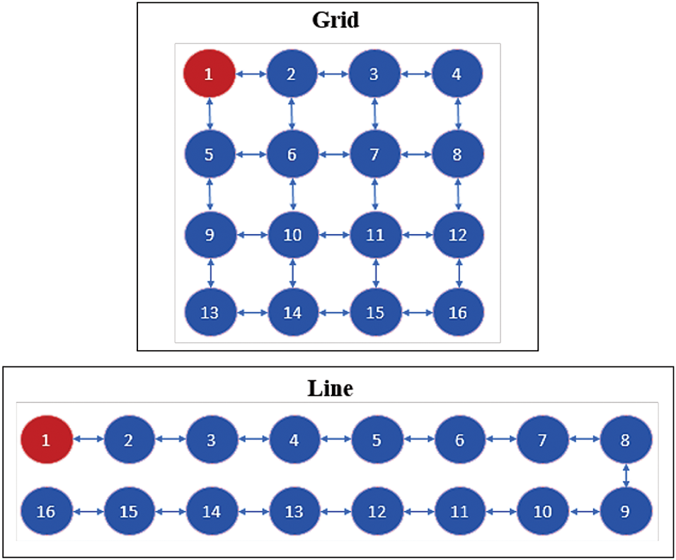
Figure 4: Layout of WSN Testbed for Experiments

6.2 Logical Clock and Frequency (Rate)

This study needs to examine the clock value discrepancies among the network nodes to assess the synchronization accuracy of each protocol. It achieves this by gathering the clock values of all nodes at each communication instant k. Specifically, during every synchronization round, each node, excluding node 1, sends its logical clock and rate values to the base station, which is connected to a computer. Each node’s clock and clock rate values are converted to decimal form and saved in a text file. The global mean logical clock, cglobal and frequency, fglobal values of experiments on the grid and line test-beds are shown in Fig. 5. The values are calculated, respectively, as

cglobal=EV[ci(tk)](46)

fglobal=EV[1/Δi(tk)](47)

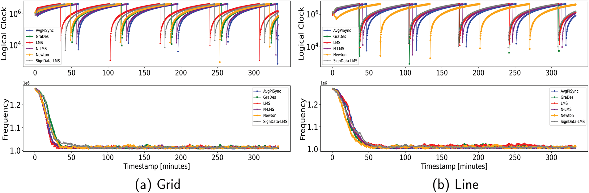
Figure 5: Average global logical clock, cglobal and frequency, fglobal values for 16 nodes grid and line test-beds. The logarithmic y-axis is used in the plots to observe the detailed changes in cglobal and fglobal values for each protocol

All protocols are observed to converge approximately to the nominal frequency of f^ = 1 MHz, although at different times. Overall, fglobal converges to f^ for protocols for the grid network at between 33−39 min and between 41–50 min for the line network. The Newton-based protocol has the fastest convergence for both networks, followed by the GraDes and AvgPISync protocols. The LMS and N-LMS protocols had similar convergence times, and the Sign-Data LMS was the slowest protocol. The mean global logical clock values, cglobal for the protocols are also observed to be within similar peak values for all but there seems to be a higher time-shift of cglobal values for the grid network than the line network.

6.3 Criteria for Synchronization Accuracy

The error between the logical clocks of arbitrary nodes, i and j, in the test network after convergence time, TC, to the experiment end time, TE, is used to assess the synchronization accuracy between all protocols for the grid and line networks.

eij(tk)=cj(tk)−ci(tk), TC≤tk≤TE(48)

Network-wide synchronization accuracy at each communication instant is then calculated using maximum global synchronization error, eglobal and the synchronization accuracy of nodes with respect to their neighbors by using the maximum local synchronization error, elocal given respectively by [20]

eglobal=EV[maxi,j∈Veij(tk)](49)

elocal=EV[maxi,j∈V,j∈𝒩ieij(tk)](50)

The synchronization accuracy between any two network nodes can be assessed using the global synchronization error, eglobal, whereas the synchronization accuracy between adjacent nodes can be assessed using the local synchronization error elocal.

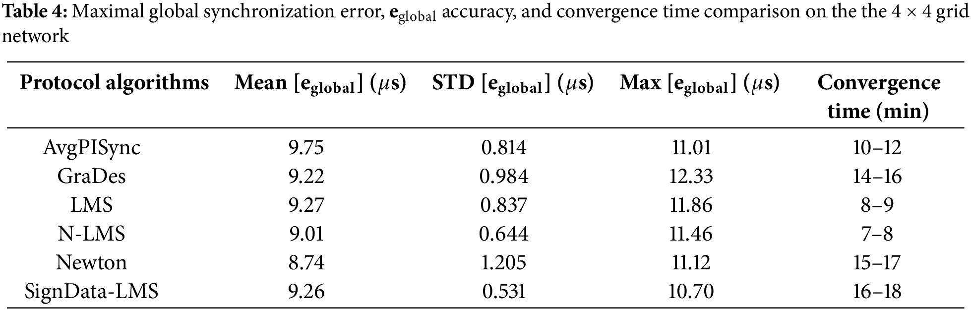
The study then computes the global error’s mean, standard deviation, and maximum statistics as key indicators of each protocol’s robustness and ability to perform in grid and line topologies. The mean error reflects the overall accuracy of the synchronization, and the standard deviation indicates the variability of the synchronization between nodes, and the maximum error highlights the worst-case performance. Consistent results across both topologies suggest that the protocol is not overfitted to specific test cases but instead demonstrates some level of adaptability and reliability. The study validates a protocol’s resilience to structural topology changes by analyzing these metrics collectively. These metrics also provide a foundation for future validation in broader real-world applications.

6.4 Experimental Results on Grid

The experimental results on the grid network for eglobal and elocal are given in Fig. 6a,b, respectively. Regarding both global and local synchronization error, all protocols, including the AvgPISync protocol, show high synchronization accuracy, with values ranging from 10.7–12.33 μs for maximal global error and 5.57–7.11 μs for maximal local error although Sign-Data LMS has the best performance for global and local errors. However, in terms of convergence time, LMS and N-LMS are the fastest to converge within 8–9 min and 7–8 min, respectively. This is followed by AvgPISync protocols, which converge within 10–12 min, then 14–16 min for the GraDes algorithm. The Newton search algorithm and Sign-Data LMS-based protocol were the slowest, with 15–18 min values.

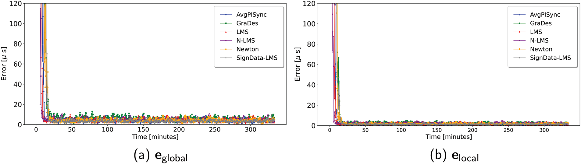
Figure 6: Global and local synchronization-error on the 4×4 grid network

In addition to the error curves, an error distribution histogram and kernel density estimation (KDE) for the probability density function (PDF) of eglobal for each protocol are carried out and shown in Fig. 7a,b, respectively. It observes a Gaussian PDF distributed eglobal for all protocols with similar performances in terms of mean and standard deviation (STD), although AvgPISync has a higher mean eglobal as compared to the stochastic gradient-based protocols. Sign-Data LMS-based protocol shows a tighter PDF curve with STD=0.531μs which is consistent with the theoretical analysis of synchronization precision. Table 4 summarizes the mean, STD, maximum, and convergence time of the global error of all tested protocols.

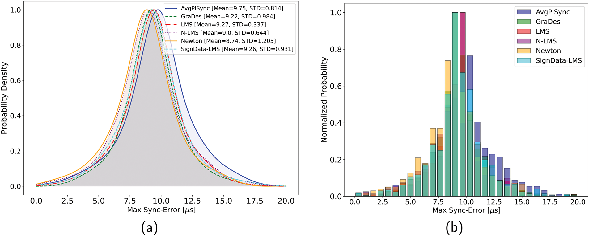
Figure 7: The (a) probability density and (b) normalized distribution histogram of the global synchronization-error, eglobal on grid network

For WSN applications on dense networks requiring rapid convergence, it might be best to consider the N-LMS-based protocol for logical clock frequency adjustments. If synchronization accuracy or precision is rather paramount with tolerable slower convergence, then it is best to use Sign-Data LMS for the frequency update. For balanced accuracy and convergence time requirements, the GraDes or Newton search algorithms can be employed, although the LMS algorithm will also perform in such a case.

6.5 Experimental Results on Line Topology

The experimental results on the line network for eglobal and elocal are given in Fig. 8a,b, respectively. First, the Newton-based protocol converges the fastest regarding global convergence time within 12–14 min. AvgPISync, then GraDes follow this, and then N-LMS and LMS-based protocols. Sign-Data LMS shows the slowest convergence time and takes nearly twice as long as the Newton search algorithm-based protocol. However, regarding synchronization accuracy, the Sign-Data LMS LMS-based protocol outperforms all protocols with maximal global and local synchronization errors of 11.08 and 8.55μs. The GraDes and LMS-based protocols also achieve good accuracy around 13μs. AvgPISync, N-LMS, and Newton algorithms also achieve an acceptable accuracy of around 15μs. In the PDF and distribution plots of eglobal shown in Fig. 9a,b, the AvgPISync shows a higher mean global error of 14.62μs than all protocols with values around 12μs. In terms of precision, the Sign-Data LMS outperforms all the other protocols with an STD of 0.9μs. Also, we observe the least precision for the AvgPISync (STD =2.436μs) protocol as compared to all other protocols (STD = 1.2–1.7 μs).

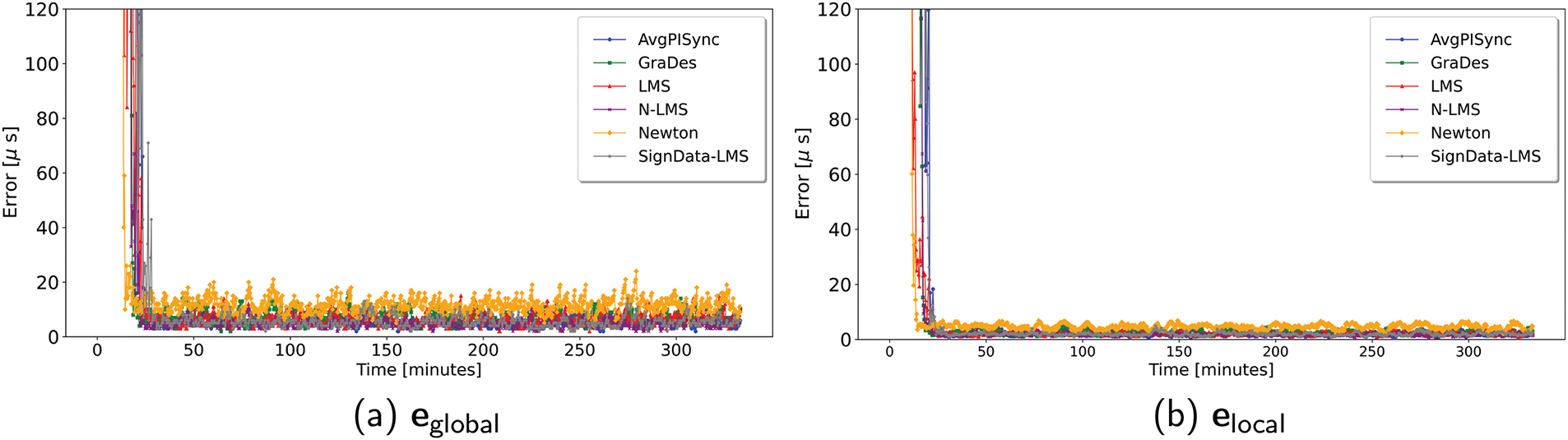
Figure 8: Global and local synchronization-error on the line network

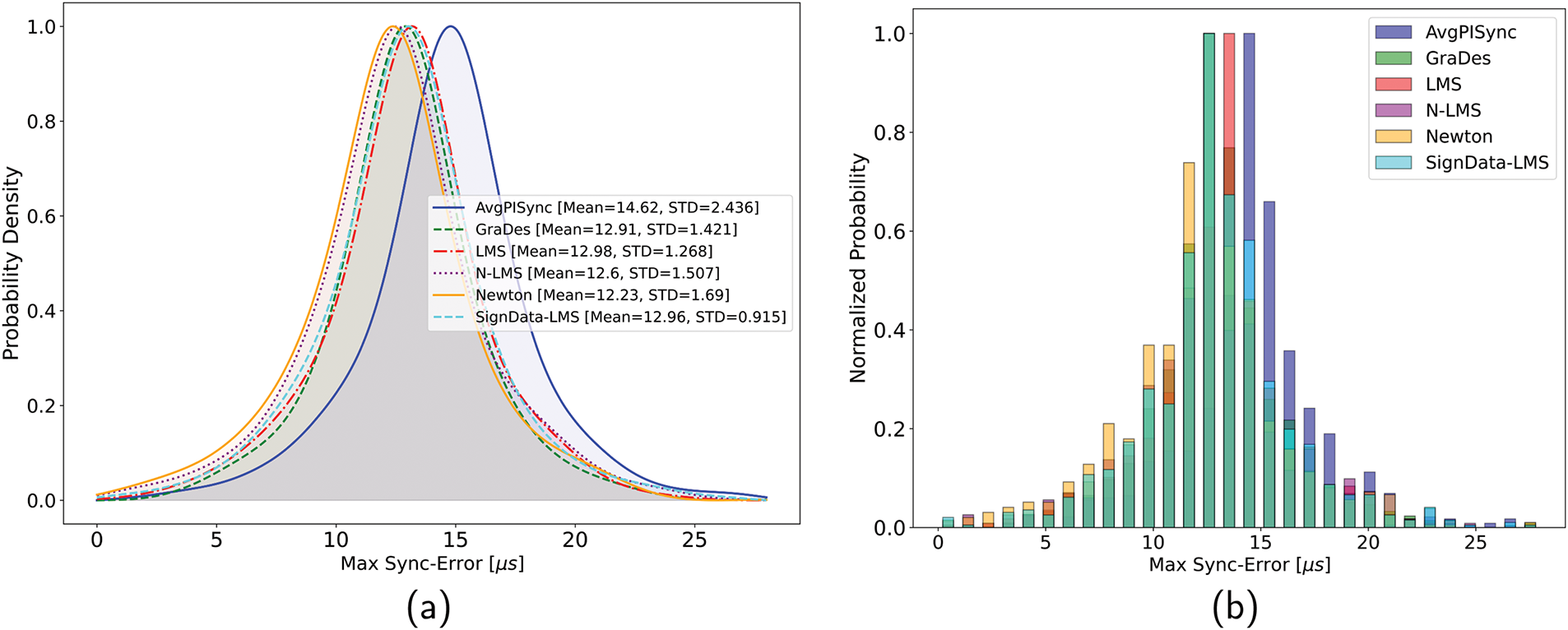
Figure 9: The (a) probability density and (b) normalized distribution histogram of the global synchronization-error, eglobal on line network

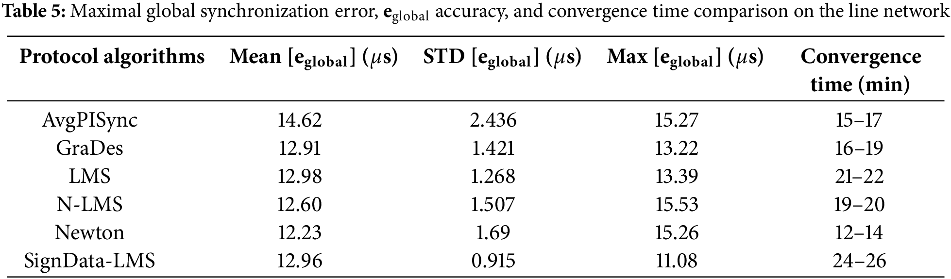
Therefore, in selecting the optimal algorithm for logical clock frequency adjustments, for WSN applications where sparse or simple type network architectures are used, if accuracy and precision are paramount over fast convergence, Sign-Data LMS is recommended; otherwise, if fast convergence is the priority, then the Newton search algorithm is preferred. For a more balanced performance, N-LMS or GraDes are recommended. A summary of the mean, STD, maximum, and convergence time of the global error of all tested protocols is shown in Table 5.

6.5.1 Implications of Protocol Performance on WSN Reliability and Efficiency

The proposed synchronization protocol enhances the reliability and efficiency of WSNs in several helpful ways:

1.    The protocol helps conserve energy, which is critical for sensor nodes operating on limited battery power, by reducing the number of resynchronization events and unnecessary communication.

2.    The protocol’s high synchronization accuracy can ensure that data from different nodes is well-aligned in time, resulting in more consistent and dependable measurements of nodes.

3.    The adaptive design of the protocol can lead to nodes adapting dynamically to harsh conditions like interference and packet loss, maintaining performance even in unpredictable environments.

4.    Scalability and Stability: The flexibility in protocol design is expected to allow it to scale smoothly with larger networks or changing topologies. This is also shown in the protocol performance on the line topology.

These conclusions are drawn from theoretical analyses and the limited experimental tests conducted in this study. Although the initial results are promising, further extensive experimental testing across a broader range of real-world scenarios is necessary to validate these claims and assess the protocol’s broader applicability and effectiveness.

7  Conclusion

This study presents an adaptive method of time synchronization for WSNs inspired by a generalized class of stochastic gradient algorithms. It develops a generalized framework for time synchronization in unstructured WSNs that allows for a trade-off between synchronization accuracy, precision, and convergence time by selecting different gradient algorithms for logical clock frequency adjustments. The generalized conditions for pairwise convergence are derived in the mean-sense, steady-state error, and clock rates. Then, synchronization precision is analyzed using closed-form relations for each proposed proto-col. The LMS, GraDes, N-LMS, Newton-search, and Sign-Data LMS algorithms are analyzed using this generalized framework. All protocols achieve zero steady-state synchronization error with high synchronization precision. A generalized protocol is developed for multi-hop synchronization and implemented on real-time WSNs. Experimental results from the protocol for some algorithms show that it outperforms the AvgPISync protocol in terms of synchronization accuracy, precision, and convergence time. Despite promising results, the proposed framework has limitations, including assumptions of stationary nodes and ideal noise conditions, which cannot be applied in real-world, dynamic environments. The framework also lacks optimization for energy efficiency, a critical factor for large-scale WSNs. Future work can involve incorporating affine stochastic algorithms for improved performance, optimizing the protocols for joint synchronization accuracy and energy efficiency, and implementing them in networks with non-stationary nodes. Additionally, addressing scalability in larger, dynamic networks while maintaining synchronization accuracy will be an important challenge.

Acknowledgement: The authors acknowledge the Department of Physics, Universiti Putra Malaysia, for providing facilities and funding for the present study.

Funding Statement: This research was funded by Universiti Putra Malaysia under a Geran Putra Inisiatif (GPI) research grant with reference to GP-GPI/2023/9762100.

Author Contributions: The authors confirm their contribution to the paper as follows: study conception, protocol design, and implementation: Ramadan Abdul-Rashid, Mohd Amiruddin Abd Rahman; data collection: Ramadan Abdul-Rashid; analysis and interpretation of results: Ramadan Abdul-Rashid, Mohd Amiruddin Abd Rahman, Kar Tim Chan, Arun Kumar Sangaiah; draft manuscript preparation: Ramadan Abdul-Rashid, Mohd Amiruddin Abd Rahman. All authors reviewed the results and approved the final version of the manuscript.

Availability of Data and Materials: The data that support the findings of this study are available from the corresponding author upon reasonable request.

Ethics Approval: Not applicable.

Conflicts of Interest: The authors declare no conflicts of interest to report regarding the present study.

Appendix A. Symbol Definitions

Appendix B. Reconfiguration of Stochastic Gradient Algorithms Based on Generalized Framework

The pairwise logical clock error when node i communicates with gateway node, G is

e(tk)=ci(tk)−τG=ci(tk)−kB−βk(A1)

e(tk)=Δi(tk)τ¯i(tk+)−τG

GraDes Algorithm

Δi(tk+1)=Δi(tk)−μ∇ei2(tk)(A2)

The gradient function is derived as follows:

∇ei(tk)=∂e2(Δi)∂Δi=2ei(tk)×∂e(Δi)∂Δi=2ei(tk)τ¯i(tk)

Δi(tk+1)=Δi(tk)−2μτ¯i(tk)ei(tk)

LMS Algorithm The general update equation for LMS can be given as

Δi(tk+1)=Δi(tk)−μ∇EΔi[ei2(tk)]

Using the orthogonality principle and simplifying,

∇EΔ[ei2(tk)]=Δi(tk)E[τ¯i2(tk)]−E[τ¯i(tk)τG]

Since we are dealing with the instantaneous values, we adopt the approximations: E[τ¯i2(tk)]≈τ¯i2(tk) and E[τ¯i(tk)τG]=τ¯i(tk)τG, which implies

∇EΔ[ei2(tk)]≈τ¯i(tk)(Δi(tk)τ¯i(tk)−τG)=τ¯i(tk)ei(tk)

Hence

Δi(tk+1)=Δi(tk)−μτ¯i(tk)ei(tk)

Newton Search Algorithm

Δi(tk+1)=Δi(tk)−μ[H(tk)]−1g(tk)(A3)

where g(tk)=∂J(Δi)∂Δi and H(tk)=∂g(Δi)∂Δi

Using (4), we derive g(tk) and H(tk) respectively as

g(tk)=2e(tk)×∂e(Δi)∂Δi=2e(tk)τ¯i(tk) and

References

1. Quattrocchi C, Furnari A, Di Mauro D, Giuffrida MV, Farinella GM. Synchronization is all you need: exocentric-to-egocentric transfer for temporal action segmentation with unlabeled synchronized video pairs. In: European Conference on Computer Vision; 2024; MiCo Milano, Italy: Springer. p. 253–70. [Google Scholar]
2. Fu S, Wu J, Zhang Q, Xie B. Robust and efficient synchronization for structural health monitoring data with arbitrary time lags. Eng Struct. 2025;322(1):119183. doi:10.1016/j.engstruct.2024.119183. [Google Scholar] [CrossRef]
3. Weng Y, Zhang Y. A survey of secure time synchronization. Appl Sci. 2023;13(6):3923. doi:10.3390/app13063923. [Google Scholar] [CrossRef]
4. Shi F, Yang SX, Tuo X, Ran L, Huang Y. A novel rapid flooding approach with real-time delay compensation for wireless-sensor network time synchronization. IEEE Transact Cybernet. 2022;52(3):1415–28. doi:10.1109/TCYB.2020.2987758. [Google Scholar] [PubMed] [CrossRef]
5. Jia XD, Cui D, Hu Y. Asynchronous broadcast-based event triggered control for discrete-time clock synchronization. IET Cont Theo Appl. 2023;17(11):1543–51. doi:10.1049/cth2.12488. [Google Scholar] [CrossRef]
6. Huan X, He H, Wang T, Wu Q, Hu H. A timestamp-free time synchronization scheme based on reverse asymmetric framework for practical resource-constrained wireless sensor networks. IEEE Transact Communs. 2022;70(9):6109–21. doi:10.1109/TCOMM.2022.3188830. [Google Scholar] [CrossRef]
7. Huan X, Chen W, Wang T, Hu H, Zheng Y. A one-way time synchronization scheme for practical energy-efficient LoRA network based on reverse asymmetric framework. IEEE Transact Commun. 2023;71(11):6468–81. doi:10.1109/TCOMM.2023.3305515. [Google Scholar] [CrossRef]
8. Zong Y, Dai X, Gao S, Canyelles-Pericas P, Liu S. PkCOs: synchronization of packet-coupled oscillators in blast wave monitoring networks. IEEE Internet Things J. 2022;9(13):10862–71. doi:10.1109/JIOT.2021.3126059. [Google Scholar] [CrossRef]
9. Maróti M, Kusy B, Simon G, Lédeczi A. The flooding time synchronization protocol. In: Proceedings of the 2nd International Conference on Embedded Networked Sensor Systems. SenSys ’04; 2004; New York, NY, USA: Association for Computing Machinery; p. 39–49. [Google Scholar]
10. Chen J, Yu Q, Zhang Y, Chen HH, Sun Y. Feedback-Based clock synchronization in wireless sensor networks: a control theoretic approach. IEEE Transact Veh Technol. 2010;59(6):2963–73. doi:10.1109/TVT.2010.2049869. [Google Scholar] [CrossRef]
11. Yıldırım KS, Kantarci A. Time synchronization based on slow-flooding in wireless sensor networks. IEEE Transact Parall Distrib Syst. 2014;25(1):244–53. doi:10.1109/TPDS.2013.40. [Google Scholar] [CrossRef]
12. Lenzen C, Sommer P, Wattenhofer R. PulseSync: an efficient and scalable clock synchronization protocol. IEEE/ACM Trans Netw. 2015;23(3):717–27. doi:10.1109/TNET.2014.2309805. [Google Scholar] [CrossRef]
13. Yıldırım KS, Carli R, Schenato L. Adaptive proportional-integral clock synchronization in wireless sensor networks. IEEE Transact Cont Syst Technol. 2018;26(2):610–23. doi:10.1109/TCST.2017.2692720. [Google Scholar] [CrossRef]
14. Lee YR, Chin WL. Low-complexity time synchronization for energy-constrained wireless sensor networks: dual-clock delayed-message approach. Peer Peer Netw Appl. 2017;10(4):887–96. doi:10.1007/s12083-016-0437-4. [Google Scholar] [CrossRef]
15. Apicharttrisorn K, Choochaisri S, Intanagonwiwat C. Energy-efficient gradient time synchronization for wireless sensor networks. In: 2010 2nd International Conference on Computational Intelligence, Communication Systems and Networks; 2010; Liverpool, UK. p. 124–9. [Google Scholar]
16. Schenato L, Fiorentin F. Average TimeSynch: a consensus-based protocol for clock synchronization in wireless sensor networks. Automatica. 2011;47(9):1878–86. doi:10.1016/j.automatica.2011.06.012. [Google Scholar] [CrossRef]
17. Maggs M, O’Keefe S, Thiel D. Consensus clock synchronization for wireless sensor networks. IEEE Sens J. 2012;12(6):2269–77. doi:10.1109/JSEN.2011.2182045. [Google Scholar] [CrossRef]
18. He J, Cheng P, Shi L, Chen J, Sun Y. Time synchronization in WSNs: a maximum-value-based consensus approach. IEEE Transact Automat Cont. 2014;59(3):660–75. doi:10.1109/TAC.2013.2286893. [Google Scholar] [CrossRef]
19. Wu J, Zhang L, Bai Y, Sun Y. Cluster-based consensus time synchronization for wireless sensor networks. IEEE Sens J. 2015;15(3):1404–13. doi:10.1109/JSEN.2014.2363471. [Google Scholar] [CrossRef]
20. Abdul-Rashid R, Al-Shaikhi A, Masoud A. Accurate, energy-efficient, decentralized, single-hop, asynchronous time synchronization protocols for wireless sensor networks. arXiv:1811.01152. 2018. [Google Scholar]
21. Al-Shaikhi A, Abdul-Rashid R, Masoud A. Asynchronous time synchronization protocol for WSNs. In: 2019 16th International Multi-Conference on Systems, Signals & Devices (SSD); 2019; Istanbul, Turkey. p. 518–23. [Google Scholar]
22. Wang F, Wu X, Liu Z. Energy efficiency time synchronization protocol for wireless sensor networks. In: 2021 40th Chinese Control Conference (CCC); 2021; Shanghai, China. p. 5649–54. [Google Scholar]
23. Phan LA, Kim T. Hybrid time synchronization protocol for large-scale wireless sensor networks. J King Saud Univ-Comput Inf Sci. 2022;34(10):10423–33. [Google Scholar]
24. Abdul-Rashid R, Abd Rahman MA. An adaptive procedure of time synchronization in unstructured multi-hop wireless sensor networks using butterfly optimization algorithm. J Phy: Conf Ser. 2024;2891:162026. doi:10.1088/1742-6596/2891/16/162026. [Google Scholar] [CrossRef]
25. Jia Z, Cui D, Dai X, Liu ZW, Liu S, Chai T. Low overhead minimum variance time synchronization for time-sensitive wireless sensor networks. IEEE Trans Autom Sci Eng. 2024;1–11. doi:10.1109/TASE.2024.3419142. [Google Scholar] [CrossRef]
26. Zong Y, Liu S, Liu X, Gao S, Dai X, Gao Z. Robust synchronized data acquisition for biometric authentication. IEEE Transacti Indust Inform. 2022;18(12):9072–82. doi:10.1109/TII.2022.3182326. [Google Scholar] [CrossRef]
27. Zong Y, Dai X, Wei Z, Zou M, Guo W, Gao Z. Robust time synchronization for industrial internet of things by h∞ output feedback control. IEEE Inter Things J. 2023;10(3):2021–30. doi:10.1109/JIOT.2022.3144199. [Google Scholar] [CrossRef]
28. Yıldırım KS. Gradient descent algorithm inspired adaptive time synchronization in wireless sensor networks. IEEE Sens J. 2016;16(13):5463–70. doi:10.1109/JSEN.2016.2555996. [Google Scholar] [CrossRef]
29. Abdul-Rashid R, Zerguine A. Time synchronization in wireless sensor networks based on newton’s adaptive algorithm. In: 2018 52nd Asilomar Conference on Signals, Systems, and Computers; 2018; Pacific Grove, CA, USA. p. 1784–8. [Google Scholar]
30. Butusov D, Rybin V, Karimov A. Fast time-reversible synchronization of chaotic systems. Phys Rev E. 2025;111(1):014213. doi:10.1103/PhysRevE.111.014213. [Google Scholar] [PubMed] [CrossRef]
31. Wei C, Wang X, Ren F, Zeng Z. Local and global finite-time synchronization of fractional-order complex dynamical networks via hybrid impulsive control. IEEE Transact Syst Man Cybernet: Syst. 2025;99:1–10. doi:10.1109/TSMC.2024.3520135. [Google Scholar] [CrossRef]
32. Hu T, Park JH, Liu X, He Z, Zhong S. Sampled-data-based event-triggered synchronization strategy for fractional and impulsive complex networks with switching topologies and time-varying delay. IEEE Transact Syst Man Cybernet: Syst. 2021;52(6):3568–80. doi:10.1109/TSMC.2021.3071811. [Google Scholar] [CrossRef]
33. Resmi NC, Chouhan S. An enhanced methodology for energy-efficient interdependent source-channel coding for wireless sensor networks. IEEE Transact Green Commun Network. 2020;4(4):1072–80. doi:10.1109/TGCN.2020.3008079. [Google Scholar] [CrossRef]
34. Gao D, Zhang S, Zhang F, He T, Zhang J. RowBee: a routing protocol based on cross-technology communication for energy-harvesting wireless sensor networks. IEEE Access. 2019;7:40663–73. doi:10.1109/ACCESS.2019.2902902. [Google Scholar] [CrossRef]
35. Aman MN, Basheer MH, Sikdar B. Two-factor authentication for IoT with location information. IEEE Inter Things J. 2019;6(2):3335–51. doi:10.1109/JIOT.2018.2882610. [Google Scholar] [CrossRef]
Cite This Article
Copyright © 2025 The Author(s). Published by Tech Science Press.
This work is licensed under a Creative Commons Attribution 4.0 International License , which permits unrestricted use, distribution, and reproduction in any medium, provided the original work is properly cited.
Downloads
Citation Tools