Bayesian Network Reconstruction and Iterative Divergence Problem Solving Method Based on Norm Minimization

1  Introduction

In today’s era of rapid development of information technology, research in network science has gradually become a key research direction in multiple fields, covering various aspects such as social networks, biological networks, economic systems, and technological systems. These complex networks are composed of a large number of nodes and their interrelationships, usually described in the form of graphs [1,2]. The topology structure and information propagation capability of a network directly affect the overall performance and effectiveness of the system [3,4]. Therefore, how to accurately model these networks and apply them to solve practical problems has become a hot topic in scientific research today. The current research results have made progress in the reconstruction of network structures. For example, Mahdavi et al. proposed a highly robust distribution network reconstruction model to address the effectiveness of distribution network reconstruction and distributed generation in reducing energy losses, in order to cope with the uncertainty of loads and power generation. The results indicated that the model was not only simple and easy to implement, but also able to find optimized solutions within a reasonable computation time, demonstrating high robustness [5]. Hasibuan et al. proposed a strategy to improve system performance by changing the original radial network topology to a ring topology for distribution network reconstruction. After reconstruction, power flow, voltage drop, power loss, and short-circuit calculations were analyzed as references for network quality assessment. The results showed that the continuity of the network was poor in the current simulation, but after reconstruction and fault testing, the network did not experience blackouts again [6]. Gholizadeh et al. proposed a model-free reinforcement learning algorithm-based approach to train agents to adopt the optimal distribution network reconstruction in a given distribution system, addressing the issue of increased power demand caused by the extensive integration of electric vehicles. A deep Q-learning-based action sampling method was developed to reduce action space and optimize loss reduction in the system [7]. Lei et al. proposed a theory based on the discrete convex hull method to address the problem of the distribution network reconstruction model. The method treated continuous parent-child relationship variables in cross-tree constraints as discrete variables to represent the discrete convex hull of the DistFlow equation. This discrete convex hull relaxation was more compact than existing relaxation techniques for distribution network reconstruction problems [8]. However, most methods have strong data dependency, high computational complexity, and are prone to overfitting and high model complexity when dealing with high-dimensional sparse data. When faced with large-scale datasets and dynamic environments, their computational efficiency and convergence characteristics often fail to meet practical needs. Therefore, the main objective of this study is to scientifically and effectively infer the dependency relationships between variables under these complex and uncertain conditions, and to optimize and reconstruct the network. The research proposes a Bayesian network reconstruction method based on norm minimization, aiming to achieve breakthroughs in reducing data dependency and model complexity, while improving the accuracy and efficiency of network reconstruction. The problems of noise, missing data and high-dimensional sparse data set solved by the research method are widely existing in all kinds of data collection and analysis. If not solved, the accuracy and reliability of the model will be directly affected, and the effectiveness of scientific research and practical application will be hindered. Secondly, in the fields of social networks, biological networks, and economic systems, the uncertainty and complexity of data are crucial to the decision-making process, so improving the accuracy of network reconstruction is of great significance for optimizing resource allocation, predicting system behavior, and achieving effective management. The high efficiency and robustness of this method provide an effective solution for solving the fundamental problems in network reconfiguration, and help to promote the theoretical development and practical application in related fields. The innovation of this paper is as follows:

(1)   A Bayesian network reconstruction method combining the characteristics of random networks and small-world networks is proposed to improve the ability to capture complex dependencies.

(2)   L1 norm is used as a regularization means to control model complexity, reduce redundant parameters, avoid overfitting, and enhance the robustness of the model.

(3)   The introduction of a real-time updated network connection mechanism in a dynamic environment improves the model’s ability to cope with changing data characteristics and ensures higher adaptability and stability.

2  Methods and Materials

2.1 Construction of Random Networks and Small-World Network Models

The Bayesian network reconstruction method based on norm minimization uses norm as a regularization tool to learn the Bayesian network structure [9]. This method aims to infer the dependency relationships between random variables in the network by optimizing the objective function, especially suitable for high-dimensional data governance and effectively controlling model complexity. Bayesian network is a directed acyclic graph used to represent and infer conditional dependencies between random variables [10]. The goal of refactoring is to determine the structure and parameters of the network, with the former representing the dependency relationships between variables and the latter representing the strength of these relationships [11]. If there is no prior knowledge, a random network model can be used as a hypothesis basis to generate the preliminary structure of the network [12]. The random network model emphasizes the independence of connections and the same connection probability by randomly connecting nodes. Its structure is shown in Fig. 1.

Figure 1: Schematic diagram of random network structure

In Fig. 1, the random network model provides a preliminary modeling approach for handling random dependencies between variables, while the Bayesian network reconstruction based on norm minimization reduces model complexity and improves accuracy through data optimization [13,14]. Random networks are mainly composed of two mechanisms: the randomness of node connections and topological characteristics. The randomness of node connections means that each pair of nodes forms a connection with the same probability; Topological characteristics indicate that many practical networks are not completely random, but have specific features such as clustering and degree distribution, which can usually be approximated by Poisson distribution, as shown in Formula (1) [15].

σ=Np(1)

In Formula (1), N represents nodes, p represents connection probability, and σ represents Poisson distribution. Poisson distribution provides a prior model for understanding and generating random networks, allowing nodes to be connected in a random manner without prior knowledge, providing a basic framework for network structure and helping to establish conditional dependencies [16]. Compared to completely random networks, small-world network models more accurately reflect the structure of many real-world networks by introducing high clustering and short path characteristics. In Bayesian network reconstruction, the small-world characteristic affects the dependency relationships between variables, especially in social or biological networks. This short path characteristic can promote efficient information dissemination and decision-making processes, thereby enhancing the practical significance of the reconstruction results [17–19]. The schematic diagram of the small-world network structure is shown in Fig. 2.

Figure 2: Schematic diagram of small-world network structure

In Fig. 2, a circular network consisting of N nodes connected to K neighboring nodes is first created. In this initial network, the path length between any two nodes is long and the clustering coefficient is high [20]. Subsequently, each edge in the circular network is randomly reconnected, and the network properties can be adjusted by adjusting the reconnection probability. When the probability of reconnection is low, the network maintains a high clustering coefficient and strong local connectivity. When the probability of reconnection increases, although the global distance shortens, the local structure still remains, resulting in the small-world effect [21]. The mathematical expression of the small-world network is shown in Formula (2) [22].

l=Nkf(Nkϕ)(2)

In Formula (2), k represents the network regularity, which is used to control local connectivity. ϕ represents the introduction of shortcut probability to influence the global topology of the network. l represents the path length, which is used to characterize the overall connection efficiency of the network. In terms of network reconstruction, the small-world feature adjusts the initial network through a random reconnection mechanism, making the reconstructed Bayesian network more in line with the actual data structure [23]. For random networks, their degree distribution can usually be described by Poisson distribution. If the average degree of the network is σ, the probability value of k is shown in Formula (3) [24].

p(k)=σke−σk!(3)

In Formula (3), σ affects the connectivity and information flow of the network. By analyzing the degree distribution, important nodes can be identified and enhanced to determine which nodes need to be prioritized for connectivity and improve network performance.

2.2 Reconfiguration and Iterative Divergence Problem Processing Based on Game Networks

In the process of constructing network models, in addition to focusing on structure and connection mechanisms, it is also necessary to effectively reconstruct and optimize network representations to extract valuable information. Especially in complex systems, the dependency relationships between variables affect information dissemination and decision-making, so it is crucial to construct Bayesian networks that can accurately reflect these relationships. The above model provides a preliminary framework for a deeper understanding of network dynamic behavior, exploring potential relationships between nodes by generating random connections [25]. The study will discuss Bayesian network reconstruction based on norm minimization. As a regularization technique, norm minimization can effectively control model complexity in high-dimensional data processing and help researchers identify key dependencies from multiple variables. In game networks, the representation of complex interdependence relationships between participants is crucial for analyzing game outcomes. Bayesian networks visually represent these conditional dependencies through directed acyclic graphs, helping to understand the mutual influence between different strategies. Norm minimization can improve the accuracy of network structure learning, thereby better describing these dependency relationships [26]. The most typical models in game networks are the Prisoner’s Dilemma Game (PDG) and the Snowdrift Game (SG), with the PDG model shown in Fig. 3 [27,28].

Figure 3: Schematic diagram of PDG model

In Fig. 3, there are two main participants, usually labeled as “Decision maker A” and “Decision maker B”. These two participants face the same decision-making scenario, which is choosing to cooperate or betray without knowing each other’s decision. Each participant’s decision usually has two options, choosing to collaborate with the other party, which usually means lower personal benefits, but both parties will gain certain benefits. Choosing to betray the other party means that if they cooperate, they will gain higher personal benefits, but if they also choose to betray, the benefits may decrease. The SG model is shown in Fig. 4.

Figure 4: Schematic diagram of SG model

In Fig. 4, the SG model is labeled as “Decision maker A” and “Decision maker B”, with each player facing the same decision, including two main options: Players clear the snow together, which usually brings common benefits; Alternatively, one party may choose not to clear the snow and instead utilize the labor of other players. This model is used to analyze the dynamic choice between cooperation and self-interest, especially for the management and utilization of public resources. In the game model, there is a pairwise game between individuals, and either party can choose two strategies: cooperative strategy or betrayal strategy. This setting helps to study the conflicts of interest and potential for cooperation in the decision-making process. When individuals in the game choose to cooperate, the study represents it through S(C)=(1,0)T. When an individual in the game chooses to betray, it is represented by S(D)=(1,0)T. The individual’s returns depend on their strategy and the choices of other participants, which are described by a return matrix as shown in Formula (4).

{PPDG=(10b0)PSG=(11−b1+b0)(4)

In Formula (4), b represents the parameter of betrayal temptation, which has a direct impact on the control strategy. Each individual engages in a game with their surrounding neighbors simultaneously, and the participants’ gains in each round are determined by their strategies and the choices of their neighbors. At this point, the formula for calculating returns not only reflects the individual’s own choices, but also takes into account the impact of local environment on the strategy. The profit for each round is shown in Formula (5).

Gi=∑j∈ΓiSiTPSj(5)

In Formula (5), Gi represents the size of the profit, S represents the game strategy, and Γ represents the set of neighbors, which reflects the influence of the local environment on the strategy. T represents the transpose function. In terms of network reconstruction, by evaluating the benefits of various strategies, optimizing the connection relationships in the network, and ensuring that each node selects the optimal strategy, dynamic output is provided for the reconstruction of Bayesian networks. After obtaining profits, individuals in the game generally update their game strategies according to the situation and continue to gain profits in subsequent games. Therefore, the probability of individuals learning the opponent’s strategy is shown in Formula (6).

W(Si←Sj)=11−exp⁡[(Gi−Gj)/κ](6)

In Formula (6), κ represents noise, and the size of the noise value determines the randomness of the game. In terms of network reconstruction, it provides a basis for dynamically updating the network structure, ensuring that the network can continuously adjust based on feedback from members to overcome possible learning stagnation or dispersion during iterations. These noises mainly come from the uncertainty and incompleteness of the data, usually generated during the game, and these noises may be hidden in the collected data, such as decision-making errors of the participants, measurement errors, or inconsistencies in individual behavior. Although these noises come from actual data, the proposed network reconstruction method makes the model pay more attention to important variable relations in the learning process by punishing redundant parameters and enhancing the sparsity of the model, avoiding overfitting the noise, thus overcoming the possible learning stagnation and divergence problems in the iterative process, and ensuring the stable convergence and performance improvement of the model.

The network reconstruction method in this paper mainly improves the capturing ability of network structure by constructing random network model and small-world network characteristics. In this process, the initial network is generated through random connections, and then the characteristics of the small-world network are used to enhance the connectivity between nodes and the efficiency of information transmission. This design allows the network to better reflect the complex dependencies in the real system, thereby reducing the risk of divergence in the application during iteration. The universality of this method is reflected in its wide application range, which is not only limited to specific types of networks, such as game networks, but also can be applied to network reconstruction in social networks, biological networks and other complex systems. Through random network generation and the introduction of small-world network, the model can adapt to various data structures and dynamic changes, and can effectively avoid iterative divergence problems in the face of complex dependency between nodes and data noise and missing.

2.3 Bayesian Network Reconstruction and Iterative Dispersion Based on Norm Minimization

Based on the above analysis, the study will delve into how to use adjacency matrices to accurately express the connection relationships between game individuals under a specific number of nodes, and reflect dynamic returns by updating network connections. When the number of network nodes is N, the expression of the adjacency matrix is N∗N. The element value of this matrix is 1, indicating that two game individuals are connected to each other, and 0 indicates that they are not connected. The benefits of individual players in the game are calculated by multiplying the adjacency matrix with the benefit vector, forming a close relationship between the network structure and the benefits, as shown in Formula (7).

Gx(t)=ax1SxT(t)⋅P⋅S1(t)+⋅⋅⋅+axNSxT(t)⋅P⋅SN(t)(7)

In Formula (7), ax represents the element value of the adjacency matrix, which clearly describes the network connection through the revenue vector and adjacency matrix, forming the relationship between the network structure and revenue. The study represents the income at a certain moment through a vector, and the specific expression is shown in Formula (8).

Gx=φx⋅Ax(8)

In Formula (8), Gx represents the revenue vector, φx represents the network matrix, and Ax represents the node connectivity. From the analysis of network reconstruction and tight mathematical expression, direct feedback of benefits can be obtained, and network connections can be updated based on the benefits. This feedback based reconstruction can significantly improve network performance. The expression for φx is shown in Formula (9).

φx=[Fx1(t1)Fx2(t1)…FxN(t1)Fx1(t2)Fx2(t2)…FxN(t2)…………Fx1(tm)Fx2(tm)…FxN(tm)](9)

In Formula (9), F represents the obtainable benefits of the game between individuals, and t represents the game time. Capturing the game dynamics that change over time helps to incorporate time factors into the network structure. After considering the change of income, adjust the connection relationship of the adjacency matrix to more truly reflect the evolution of network reconfiguration under different conditions. By using Formulas (7) to (9), the benefits of each individual in specific game situations can be obtained in a timely manner. This feedback mechanism enables the network to self adjust its connections to adapt to changes in the environment and the evolution of strategies. This dynamic update enables the network structure to become more realistic over time, thereby alleviating the iterative dispersion caused by information delay or external changes. In practical applications, the connections of most networks are sparse, and many nodes have connections close to zero with other nodes. To address this issue, research can adopt compressive sensing methods. Compressed sensing is a mathematical technique that can efficiently reconstruct signals in situations where information is sparse, resulting in Formula (10).

Gx=φx⋅Ax=min‖Ax‖0(10)

In Formula (10), ‖⋅‖0 represents the L0 norm, which is mainly used to express the number of non-zero elements in Ax.

Due to the fact that directly solving Formula (7) is an NP hard problem and computationally complex, the study introduces another norm L1 to replace the original expression, in order to transform the problem into a more manageable convex optimization problem. Formula (11) provides a clear expression for achieving this optimization.

Gx=φx⋅Ax=min‖Ax‖1(11)

In Formula (11), ‖⋅‖1 represents the L1 norm, and the calculation of ‖Ax‖1 is shown in Formula (12).

‖Ax‖1=∑i=1N|Axi|(12)

Formulas (10) to (12) can improve the convergence and computational efficiency of the model by controlling sparsity and reducing unnecessary complexity. The sparsity in the optimization process ensures a concise network structure, avoids overfitting and instability, and thus improves the stability and convergence of iterations. In summary, the proposed network reconstruction flowchart is shown in Fig. 5.

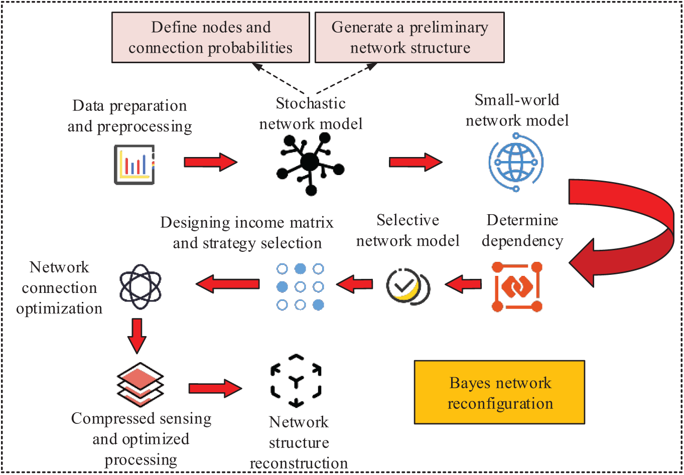
Figure 5: Network reconstruction flowchart

In Fig. 5, the specific process is as follows: Before building the model, it is necessary to prepare and preprocess the input data, including data cleaning and missing value processing, to ensure the effectiveness of the analysis. Based on the predetermined number of nodes and connection probabilities, generate a preliminary random network structure as a preliminary modeling of the random dependencies between variables for subsequent analysis. On this basis, a small number of random rewiring can adjust the network to small-world characteristics, improve network aggregation and reduce path length, and more accurately reflect the real-world network structure. The small-world network structure is used to further reconstruct the Bayesian network, with a focus on determining the dependency relationships between nodes, in order to analyze the strategic choices and mutual influences of participants. A revenue matrix is constructed and the revenue of each node is calculated, the network connection relationship is updated by multiplying the adjacency matrix with the revenue vector, in order to optimize the strategy and improve overall performance. To solve the problem of network sparsity, compressive sensing technology is adopted to transform it into a manageable convex optimization problem, ensuring the simplicity and stability of the network structure and avoiding overfitting. The final output is the complete Bayesian network structure, extracting key dependency relationships to provide support for subsequent decision-making and inference.

The Bayesian network reconstruction method based on norm minimization is introduced in the above content, which is complementary to stochastic network modeling. Stochastic network modeling pays more attention to the initial construction and structural adjustment of the network, and focuses on how to generate the network shape that can reflect the actual situation. In addition, L1 norm minimization is introduced as a regularization technique to comprehensively improve the stability and accuracy of the model in variable dependence inference by optimizing complexity.

3  Results

3.1 Analysis of Game Network Reconstruction and Iterative Divergence Problems

The efficacy of the proposed method is verified by using the MATLAB experimental platform. The three strategies of chess network, small-world network and norm minimization are actually complementary to each other, and together they constitute the complete network reconstruction method proposed. The game network offers a tangible application scenario, demonstrating the method’s capability in modeling complex dependencies by examining participant decision-making and interactions. Small-world network introduces high aggregation and short path characteristics, bringing the network structure closer to real-world complexity, facilitating rapid information dissemination and connectivity, thus further strengthening the model’s stability. Finally, norm minimization, as a regularization technique, manages model complexity, mitigates overfitting, and addresses divergence issues during iteration. The research mainly used a Bayesian framework generated by random networks to reconstruct and analyze game networks and small-world networks, assessing the method’s utility comprehensively through two dimensions: the amount of data required for reconstruction and the convergence performance of the algorithm. In terms of evaluation metrics, two key indicators was set: Successful Reconstruction Rate of Existing Links (SREL) and Successful Reconstruction Rate of Non-Exiting Links (SRNL). SREL measures the ability of reconstruction algorithms to successfully identify connections that actually exist in a network. The importance of this indicator lies in its ability to reflect the performance of algorithms in real network structures, providing a direct quantitative basis for understanding the effectiveness of algorithms. SRNL evaluates the algorithm’s ability to correctly identify non connections in the absence of connections in the network. A high SRNL value indicates that the algorithm can effectively eliminate connections that should not exist, thereby enhancing the credibility of the model. Meanwhile, the study employed Sparse Bayesian Learning Network (SBLN) for comparative validation. Assuming the number of network nodes is 200 and the probability of any connection between two points is 0.1, the reconstruction results of the game network by the two models are shown in Fig. 6.

Figure 6: Reconstruction structure of game network

Fig. 6a,b respectively shows the reconstruction results of PDG with L1 norm minimization and SBLN. Among them, the SRNL value of L1 norm minimization and SBLN maintained at almost 100% for any amount of data. When the SREL of both models reached 100%, the minimum data required for the L1 norm minimization model was about 40%, and the minimum data required for SBLN was about 45%. Fig. 6c,d respectively shows the reconstruction results of SG with L1 norm minimization and SBLN. When the SREL with minimized L1 norm reached 100%, the minimum required data was about 39%. When the SREL of SBLN reached 100%, the minimum required data was about 46%. The results indicated that the method based on norm minimization was superior to SBLN in terms of data efficiency and could achieve the same reconstruction performance with relatively less data. The comparison results of the operating efficiency of different methods are shown in Fig. 7.

Figure 7: Comparison of operational efficiency of different methods in game networks

The results in Fig. 7 show that the L1 norm minimization network maintained a running efficiency of around 1.0 s under different data volumes. The operational efficiency of SBLN was inversely proportional to the amount of data, with more data resulting in longer runtime. When the data volume was about 97%, the running time of SBLN was about 13.2 s. The results showed that the L1 norm minimization model could quickly converge to the optimal solution in each iteration, indicating that it could save time and computational resources when dealing with complex iterative discrete problems. In practical situations, the influence of noise is ubiquitous. Therefore, the study analyzed the network reconstruction results by introducing different signal-to-noise ratio models, as shown in Fig. 8.

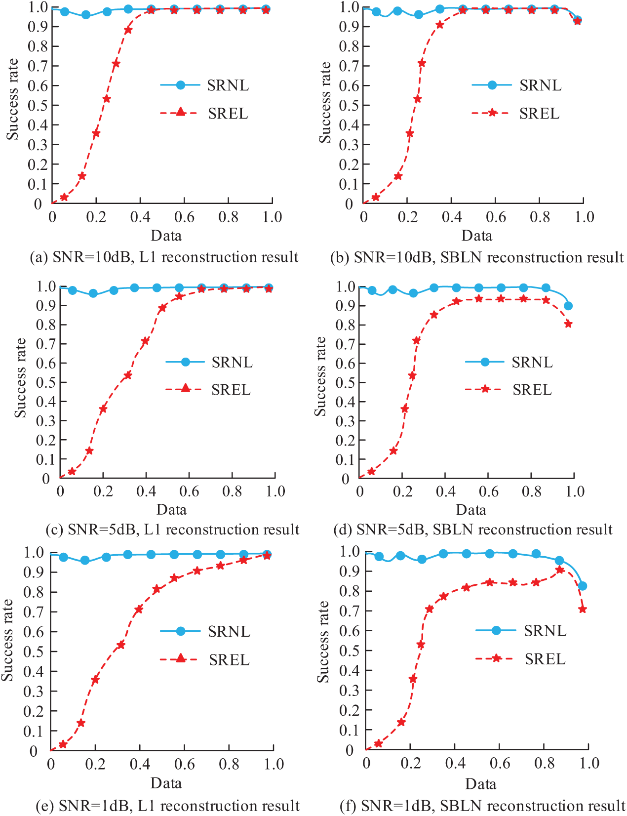
Figure 8: Reconstruction results under different signal-to-noise ratio environments

Fig. 8a,b shows the reconstruction results of L1 arithmetic minimization and SBLN in a 10 dB environment. The results showed that SRNL with minimized L1 norm reached 100%, requiring approximately 40% of the data volume. When the SREL of SBLN reached 100%, it required about 48% of the data volume, and when the data volume reached 80%, the SREL results decreased, with a final success rate of only 90%. Fig. 8c,d shows the reconstruction results in a 5 dB environment, where 80% of the data was required to achieve 100% SREL for L1. The highest success rate of SREL in SBLN was 90%, and a data volume of 90% was required at this time. If the data volume exceeded 90%, the success rates of SRNL and SREL decreased to 75% and 72%, respectively. Fig. 8e,f shows the reconstruction results in a 1 dB environment, where 100% of the data was required for L1’s SREL to reach 100%. The highest success rate of SREL in SBLN was 80%, and at this time, a data volume of 80% was required. When the data volume reached 100%, the SRNL and SREL success rates of SBLN were 72% and 73%, respectively. The results indicated that both L1 and SBLN could be successfully reconstructed in high signal-to-noise ratio environments, which might be attributed to the small interference caused by noise during the model iteration process, thus both could converge well. As the signal-to-noise ratio decreased, the interference of noise increased, and the required number of iterations also increased, resulting in a significant decrease in the success rate of SBLN, indicating that there might be a risk of divergence during the iteration process.

3.2 Analysis of Small-World Network Reconstruction and Iterative Divergence Problems

The study reconstructed the small-world network using PDG data and SG data without considering noise, and the results are shown in Fig. 9. Fig. 9a,b respectively shows the reconstruction results of L1 norm minimization and SBLN on small-world networks under PDG data. Among them, when the SREL of both models reached 100%, the minimum data required for the L1 norm minimization model was about 34%, and the minimum data required for SBLN was about 37%. Fig. 9c,d respectively shows the results of L1 norm minimization and SBLN reconstruction of SG data. When the SREL with minimized L1 norm reached 100%, the minimum required data was about 31%. When the SREL of SBLN reached 100%, the minimum required data was about 34%. Small-world networks typically have high clustering and short path characteristics. The successful reconstruction of L1 norm minimization in such networks means that this method can effectively capture the local connectivity and global structure between nodes, thereby preserving these key characteristics in network modeling.

Figure 9: Small-world network reconstruction based on game data

The efficiency results of the two methods under different data are shown in Fig. 10. The results in Fig. 10 show that the L1 norm minimization network maintained a running efficiency of around 2.0 s with a small fluctuation range. The operational efficiency of SBLN showed significant changes, with a data volume of less than 20% and an operational efficiency of less than 2.0 s. After the data volume reached 20%, the running efficiency was higher than 2.0 s, and when the data volume was 98%, the running efficiency was 11.3 s. The minimization of L1 norm had a low computational complexity during the iteration process and could efficiently and stably handle data of different scales. This stability greatly reduced the divergence risk that might occur during the iteration process.

Figure 10: Comparison of operational efficiency of small world network reconstruction

The network reconstruction under different signal-to-noise ratio environments is shown in Fig. 11. Fig. 11a,b shows the reconstruction results of L1 arithmetic minimization and SBLN in a 15 dB environment. The results showed that SRNL with minimized L1 norm reached 100%, requiring approximately 45% of the data volume. The highest SREL value of SBLN was 95%. Fig. 11c,d shows the reconstruction results in a 10 dB environment, with the highest success rate of SREL for L1 being 98%. The highest success rate of SREL in SBLN was 90%. Fig. 11e,f shows the reconstruction results in a 5 dB environment, with the highest success rate of SREL for L1 being 96% 1. The highest SREL success rate in SBLN was 90%, and when the data volume reached 100%, the SRNL and SREL success rates of SBLN were 68% and 68%, respectively. The results indicated that minimizing the L1 norm exhibited better stability and relatively lower iteration divergence risk when facing the influence of noise.

Figure 11: Network reconstruction results in different signal-to-noise ratio environments

3.3 Analysis of Bayesian Reconstruction Examples Based on Norm Minimization

To further validate the performance of the proposed reconstruction method, the study analyzed it through actual cases. The reconstructed data set was derived from a 17.6 km long passenger-cargo common track, using total station data collected at 623 measurement points. These measuring points are evenly distributed along the railway, covering the track status under different terrain and environmental conditions. The reason why this data set is suitable for experimental testing is that it truly reflects the operating conditions of the railway and includes noise and uncertainties that may occur in the actual measurement process, such as measurement errors and changes in environmental factors. This provides a rich data source for the proposed network reconstruction method, which can effectively verify the model’s ability to deal with complex dependencies and data incompleteness, so as to ensure that the reconstruction results have practical significance and application value. The study compared the traditional Bayesian network with the SBLN model and analyzed the corresponding iteration times, maximum lift and drop amount, objective function value, and mean square error (MSE) of the model. The results are shown in Table 1.

The results in Table 1 show that the research method had 27 iterations, which significantly reduced the computational complexity and running time of the model compared to the traditional Bayesian network’s 83 iterations and SBLN’s 46 iterations. The maximum lift and drop track of the research method was 0.08, which demonstrated the robustness of the research method in handling outliers compared to the traditional Bayesian network’s 0.13 m and SBLN’s 0.10 m. The objective function value of the research method was 2883.84 cm2, which was much lower than the traditional Bayesian network’s 4883.51 cm2 and SBLN’s 4116.23 cm2. This indicates that the research method had more effectively achieved the objective function in the optimization process, with a higher degree of optimization, and could better reflect the characteristics of the data. The mean square error of the research method was 5.74 cm2, which was better than the traditional Bayesian network’s 10.81 cm2 and SBLN’s 9.25 cm2, indicating that the research method could better reduce errors when fitting the model. Further research was conducted to validate the evaluation indicators, and the overall railway alignment and the distribution of lift and drop track volume are shown in Fig. 12.

Figure 12: Overall railway alignment and distribution of lift and drop track using different methods

Fig. 12a–c respectively shows the lift and drop lane results of traditional Bayesian, SBLN, and research methods. The results showed that the lift and drop track of the research method was usually concentrated between −2 and 2 cm, showing an overall effect close to zero, indicating that the model fitted well and the lift and drop track was basically symmetrically distributed. SBLN showed significant deviation at the middle measuring point, and the lift and drop track was usually concentrated between −10 and 10 cm. The overall performance of traditional Bayesian networks was poor. Therefore, the method proposed by the research could effectively reduce the impact of outliers on the overall effect of data fitting and reconstruction, making the reconstructed line more in line with actual measurement data. The extreme values and point distribution of lift and drop volumes for different models are shown in Fig. 13.

Figure 13: Extreme values and point distribution of lift and drop tracks for different models

Fig. 13a shows the extreme values and point distribution results of the SBLN model’s lift and drop clearance. The results showed that an extreme average value of −1.22 cm was found in the second axis, indicating that the algorithm was greatly affected by outliers, leading to overall fitting deviation. Fig. 13b shows the results of the extreme values and point distribution of the lift and drop track quantities in the research method. The results showed that the average lift and drop track quantities of each segment of the model approach zero, and the number of measurement points in each segment was relatively uniform, indicating that the overall lift and drop track quantities showed a symmetrical distribution in the positive and negative directions, demonstrating the good performance of the model in suppressing bias. The frequency distribution results of different models for lift and drop tracks are shown in Fig. 14.

Figure 14: Frequency distribution results of different models for lift and drop track volume

Fig. 14a shows the frequency distribution of lift and drop tracks for the research method, with a median of 0.21 cm and relatively concentrated upper and lower quartiles. This indicates that the distribution of lift and drop tracks is generally symmetrical, with most measurement points concentrated between −6 and 6 cm, exhibiting low volatility and good stability, making it more robust in handling outliers. Fig. 14b shows the frequency distribution of the lift and drop tracks of SBLN. The results show that the median of SBLN was −0.27 cm, indicating a negative bias, and its extreme values, with a maximum value of 10.67 cm and a minimum value of −9.34 cm, are significantly higher than the research method, reflecting its vulnerability to noise. Therefore, research methods have better application effects in practical network reconstruction and iterative discretization problems. In order to further verify the effectiveness of this method, dynamic networks are incorporated into the reconstruction process. Specifically, the research constantly updates the connections between nodes based on data collected over time, which allows the model to adapt to any evolving environment. By regularly adjusting the network structure, the research will be able to capture the dynamic characteristics of the dependencies between nodes over time, thereby improving the adaptability and accuracy of the network. Therefore, the model was validated using Arabidopsis data sets. The Arabidopsis dataset is to transfer artificially cultivated Arabidopsis seedlings to a periodic light and dark environment, and sample 12–13 sample data at a 4-h interval. In a comparison experiment, a Non-homogeneous Dynamic Bayesian Network (NH-DBN) and Hidden Markov Dynamic Bayesian Networks based on Edge Coupling (EC-HMDBN) were compared, and the experimental results were shown in Table 2. The performance of different models was evaluated using the Area Under the Curve (AUC) metric.

Based on the results presented in Table 2, the comparison of the proposed research method with NH-DBN and EC-HMDBN shows notable findings regarding their performance in processing the Arabidopsis dataset. The proposed research method demonstrated the highest and most stable AUC values, peaking at 0.9710 during the 6000 iterations, indicating its strong capability in accurately capturing the underlying patterns in the sampled data. Even with slight variations across different iterations, the AUC values remained consistently high, suggesting that the model effectively handles the dynamic nature of the data. In contrast, the NH-DBN model exhibited lower AUC values compared to the proposed method, with a maximum AUC of 0.9473 at 6000 iterations. While this indicates a good performance, it was not as robust or stable as the research method. The EC-HMDBN, on the other hand, consistently recorded the lowest AUC values across all iterations, with its highest reaching only 0.8146. This suggests that EC-HMDBN may not be as effective for this specific dataset. Overall, the results highlight the effectiveness and robustness of the proposed research method in modeling the Arabidopsis dataset, significantly outperforming existing techniques (NH-DBN and EC-HMDBN) and showing promise for applications requiring accurate dynamic analyses.

4  Discussion

Through the above experimental verification, the research method demonstrated excellent reconstruction effects in the experiment of game network reconstruction. When SREL reached 100%, the minimum amount of data required for the L1 norm minimization model was 40%, while the SBLN model required 45%. This improvement in data efficiency indicated that minimizing the L1 norm not only effectively controlled the complexity of the model, but also improved reconstruction efficiency by accurately identifying the dependencies between variables. The importance of this research result lies in its provision of effective solutions for reconstructing game models facing high-dimensional and complex structures, which can improve the accuracy of strategic decision-making. In the reconstruction of small world networks, the L1 norm minimization model required a minimum data volume of 34%, which was more advantageous than SBLN’s 37%. This indicates that the model with minimized L1 norm has significant effects in capturing network structural features and improving the overall information propagation efficiency of the network. The success of this method lies in effectively capturing the interaction characteristics and information flow process between nodes, which means that in complex interwoven networks such as social networks and ecosystems, models based on this method will be more reliable and effective. In practical case analysis, the method used in the study achieved a maximum lift and drop track of 0.08 m and MSE of 5.74 cm2 when processing data from 623 measurement points. Compared with traditional Bayesian networks and SBLN, the maximum lift and drop track was 0.13 m and 10.81 cm2, and 0.10 m and 9.25 cm2, respectively, showing significant improvements. The research method introduced the Bayeisan framework and sparsity constraints structurally, enabling the model to not only efficiently capture variable features, but also demonstrate better robustness in the face of possible outliers and uncertainties in actual data. In similar studies, Parihar et al. proposed a hybrid of two metaheuristic techniques for minimizing power loss in radial distribution networks. This method used particle swarm optimization to determine the optimal allocation of multiple distributed generators, and then applied plant growth simulation algorithms for optimal network reconstruction. Research showed that the combination of penetration of multiple distributed generators and network reconstruction enabled the network to operate successfully under different load conditions without violating constraints, resulting in excellent results [29]. The computational complexity and sensitivity to initial conditions of the Parihar research model may lead to insufficient adaptability when there was limited input data or changes in conditions. The Bayesian network reconstruction method based on L1 norm minimization in this study can have higher flexibility and accuracy in small sample sizes, and is more adaptable to the complex and dynamic characteristics of social and biological networks. Gallego et al. proposed a mixed integer linear programming model to improve the performance of power distribution networks, which was used to simultaneously solve the problems of distribution network reconstruction and optimal capacitor placement. This scheme optimized by changing the system topology and determining the position and specifications of capacitors, while ensuring a global optimal solution. Compared with metaheuristic techniques applied for the same purpose, it had higher computational efficiency [30]. However, its accurate representation and efficiency in solving models are limited by its linear programming characteristics, and may not perform as well as the L1 norm method in nonlinear or high-dimensional scenarios. In addition to structural flexibility, the method based on norm minimization provides stronger generality, is suitable for the reconstruction and analysis of various complex network types, and is more efficient in model training and practical applications.

5  Conclusion

With the increasing complexity of social and biological networks, accurately reconstructing network models has become particularly important. A Bayesian network reconstruction method based on norm minimization has been proposed, which effectively captures complex dependency relationships between variables by constructing a preliminary random network and improving it into a small world network. Through experimental verification, the research method achieved good performance, indicating that the structure of the L1 norm minimization model is centered on sparsity. By introducing the L1 regularization term, the generation of redundant parameters was effectively suppressed, encouraging the model to retain only the most informative features when selecting variables. The characteristics of scale-free networks made the connections between nodes no longer simply random but enhanced the preservation of local structures. This structural optimization combined with the L1 norm method enabled the model to retain local connectivity while also possessing strong global structural understanding ability. By introducing incomplete connectivity, it enhances the fitting ability of complex real-world networks.

Although the network reconstruction method proposed in this paper has obvious advantages in solving noise, missing data, and high-dimensional sparse data sets, it also has certain limitations. Especially in dynamic environments, models may not be able to effectively deal with data characteristics and structures that change over time, and therefore may face problems of reduced efficiency and reliability. In addition, the effect of different types of noise on the reconstruction results is not fully considered, which will lead to the degradation of model performance in some application scenarios. Therefore, the adaptive updating mechanism can be introduced in future research, so that the model can adjust the network structure and parameters dynamically according to the new data. Secondly, the noise modeling and classification of the system are carried out, and the corresponding processing strategies are adopted according to different noises. In addition, ensemble learning is used to combine the outputs of multiple models to improve overall predictive performance and robustness. Finally, the feedback mechanism is designed so that the model can be dynamically optimized according to the output quality, thus improving the adaptability and performance of the model in complex and changeable environment.

Acknowledgement: This work is supported by the Scientific and Technological Developing Scheme of Jilin Province, China, and the National Natural Science Foundation of China.

Funding Statement: This work is supported by the Scientific and Technological Developing Scheme of Jilin Province, China (No. 20240101371JC), and the National Natural Science Foundation of China (No. 62107008).

Author Contributions: Kuo Li: Conceptualization, Validation, Visualization, Writing—original draft. Aimin Wang: Methodology, Supervision, Writing—review and editing. Limin Wang: Supervision, Writing—review and editing. Yuetan Zhao: Formal analysis, Project administration. Xinyu Zhu: Formal analysis, Project administration. All authors reviewed the results and approved the final version of the manuscript.

Availability of Data and Materials: The datasets generated and/or analyzed during the current study are available from the corresponding author on reasonable request.

Ethics Approval: Not applicable.

Conflicts of Interest: The authors declare no conflicts of interest to report regarding the present study.

References

1. Li Q, Chen H, Koenig BC, Deng S. Bayesian chemical reaction neural network for autonomous kinetic uncertainty quantification. Phys Chem Chem Phys. 2023;25(5):3707–17. doi:10.1039/D2CP05083H. [Google Scholar] [PubMed] [CrossRef]

2. Zemplenyi M, Miller JW. Bayesian optimal experimental design for inferring causal structure. Bayesian Anal. 2023;18(3):929–56. doi:10.1214/22-BA1335. [Google Scholar] [CrossRef]

3. Zeng J, Todd MD, Hu Z. Probabilistic damage detection using a new likelihood-free Bayesian inference method. J Civ Struct Health Monit. 2023;13(2):319–41. doi:10.1007/s13349-022-00638-5. [Google Scholar] [CrossRef]

4. Yuchi HS, Mak S, Xie Y. Bayesian uncertainty quantification for low-rank matrix completion. Bayesian Anal. 2023;18(2):491–518. doi:10.1214/22-BA1317. [Google Scholar] [CrossRef]

5. Mahdavi M, Schmitt KEK, Jurado F. Robust distribution network reconfiguration in the presence of distributed generation under uncertainty in demand and load variations. IEEE Trans Power Deliv. 2023;38(5):3480–95. doi:10.1109/TPWRD.2023.3277816. [Google Scholar] [CrossRef]

6. Hasibuan A, Kartika K, Mahfudz S. Network Reconfiguration of 20 kV sample connection substance LG-04 lhokseumawe city using digsilent power factory 15.1. Int J Adv Data Inf Syst. 2022;3(1):20–9. doi:10.25008/ijadis.v3i1.1232. [Google Scholar] [CrossRef]

7. Gholizadeh N, Kazemi N, Musilek P. A comparative study of reinforcement learning algorithms for distribution network reconfiguration with deep Q-learning-based action sampling. IEEE Access. 2023;11:13714–23. doi:10.1109/ACCESS.2023.3243549. [Google Scholar] [CrossRef]

8. Lei C, Bu S, Zhong J, Chen Q, Wang Q. Distribution network reconfiguration: a disjunctive convex hull approach. IEEE Trans Power Syst. 2023;38(6):5926–9. doi:10.1109/TPWRS.2023.3304132. [Google Scholar] [CrossRef]

9. Schmidt M, Murphy K, Fung G, Rosales R. Structure learning in random fields for heart motion abnormality detection. IEEE Trans Pattern Anal Mach Intell. 2008;30(12):2302–16. doi:10.1109/CVPR.2008.4587367. [Google Scholar] [CrossRef]

10. Gunturi SK, Sarkar D. Network reconfiguration for searching maximum loading capacity radial network: an efficient graph theory-based machine learning approach. IETE J Res. 2024;70(3):2673–83. doi:10.1080/03772063.2023.2175049. [Google Scholar] [CrossRef]

11. Li J, Wang G, Tang T, Fan J, Liu S, Lin Z. Optimization of distribution network reconfiguration based on Markov chain Monte Carlo method. Energy Rep. 2022;8(8):679–85. doi:10.1016/j.egyr.2022.05.156. [Google Scholar] [CrossRef]

12. Yue D, He Z, Dou C. Cloud-edge collaboration-based distribution network reconfiguration for voltage preventive control. IEEE Trans Ind Inform. 2023;19(12):11542–52. doi:10.1109/TII.2023.3247028. [Google Scholar] [CrossRef]

13. Wang H, Lu H, Sun K, Wu X, He Y, Du X. Reliability evaluation method for distribution network with distributed generations considering feeder fault recovery and network reconfiguration. IET Renew Power Gener. 2023;17(14):3484–95. doi:10.1049/rpg2.12863. [Google Scholar] [CrossRef]

14. Omogoye SO, Folly KA, Awodele KO. A comparative study between Bayesian network and hybrid statistical predictive models for proactive power system network resilience enhancement operational planning. IEEE Access. 2023;11:41281–302. doi:10.1109/ACCESS.2023.3263490. [Google Scholar] [CrossRef]

15. Zhang T, Zhu P, Lu F. Stochastic reconstruction of porous media based on attention mechanisms and multi-stage generative adversarial network. Comput Geosci. 2023;27(3):515–36. doi:10.1007/s10596-023-10208-3. [Google Scholar] [CrossRef]

16. Xin J, Wang M, Qu L, Chen Q, Wang W, Wang Z. BIC-LP a hybrid higher-order dynamic Bayesian network score function for gene regulatory network reconstruction. IEEE/ACM Trans Comput Biol Bioinform. 2024;21(1):188–99. doi:10.1109/TCBB.2023.3345317. [Google Scholar] [PubMed] [CrossRef]

17. Fan Q, Li Q, Chen Y, Tang J. Modeling COVID-19 spread using multi-agent simulation with small-world network approach. BMC Pub Heal. 2024;24(1):672. doi:10.1186/s12889-024-18157-x. [Google Scholar] [PubMed] [CrossRef]

18. Watts DJ, Strogatz SH. Collective dynamics of ‘small-world’ networks. Nature. 1998;393(6684):440–2. doi:10.1038/30918. [Google Scholar] [PubMed] [CrossRef]

19. Dalgaty T, Moro F, Demirağ Y, De Pra A, Indiveri G, Vianello E, et al. Mosaic: in-memory computing and routing for small-world spike-based neuromorphic systems. Nature. 2024;15(1):142. doi:10.1038/s41467-023-44365-x. [Google Scholar] [PubMed] [CrossRef]

20. Luo G, Blumenthal M, Heide M, Uecker M. Bayesian MRI reconstruction with joint uncertainty estimation using diffusion models. Magn Reson Med. 2023;90(1):295–311. doi:10.1002/mrm.29624. [Google Scholar] [PubMed] [CrossRef]

21. Castelletti F, Peluso S. Bayesian learning of network structures from interventional experimental data. Biometrika. 2024;111(1):195–214. doi:10.1093/biomet/asad032. [Google Scholar] [CrossRef]

22. Safaei F, Hashemi Z, Emadi Kouchak MM. Analytical modeling of robustness and stochastic resilience of temporal small-world complex networks. J Comput Sci. 2024;78:102264. doi:10.1016/j.jocs.2024.102264. [Google Scholar] [CrossRef]

23. Silva YL, de Andrade Costa A. Periodic boundary condition effects in small-world networks. Eur Phys J B. 2024;97(7):105. doi:10.1140/epjb/s10051-024-00746-9. [Google Scholar] [CrossRef]

24. Ameur H, Njah H, Jamoussi S. Merits of Bayesian networks in overcoming small data challenges: a meta-model for handling missing data. Int J Mach Learn Cybern. 2023;14(1):229–51. doi:10.1007/s13042-022-01577-9. [Google Scholar] [CrossRef]

25. Li S, Cheng L, Zhang T, Zhao H, Li J. Graph-guided Bayesian matrix completion for ocean sound speed field reconstruction. J Acoust Soc Am. 2023;153(1):689. doi:10.1121/10.0017064. [Google Scholar] [PubMed] [CrossRef]

26. Agnes P, Albuquerque IFM, Alexander T, Alton AK, Ave M, Back HO, et al. Search for low mass dark matter in DarkSide-50: the Bayesian network approach. Eur Phys J C. 2023;83(4):322. doi:10.1140/epjc/s10052-023-11410-4. [Google Scholar] [CrossRef]

27. Nowak MA, May RM. Evolutionary games and spatial chaos. Nature. 1992;359(6398):826–9. doi:10.1038/359826a0. [Google Scholar] [CrossRef]

28. Pereira FB, Ferreira RS, Alencar DSM, Alves TFA, Alves GA, Lima FWS, et al. Social dilemmas, network reciprocity, and small-world property. Phys A Stat Mech Appl. 2024;655:130184. doi:10.1016/j.physa.2024.130184. [Google Scholar] [CrossRef]

29. Parihar SS, Malik N. Network reconfiguration in the presence of optimally integrated multiple distributed generation units in a radial distribution network. Eng Optim. 2024;56(5):679–99. doi:10.1080/0305215X.2023.2187790. [Google Scholar] [CrossRef]

30. Gallego LA, López-Lezama JM, Carmona OG. A mixed-integer linear programming model for simultaneous optimal reconfiguration and optimal placement of capacitor banks in distribution networks. IEEE Access. 2022;10(2):52655–73. doi:10.1109/ACCESS.2022.3175189. [Google Scholar] [CrossRef]