Applications of Advanced Optimized Neuro Fuzzy Models for Enhancing Daily Suspended Sediment Load Prediction

1  Introduction

1.1 Background, Importance, and Knowledge Gaps

Accurate suspended sediment load (SSL) prediction is crucial for hydrological modeling, water resource management, and flood control. Sediment transport affects the design and operation of dams, reservoirs, and irrigation systems, and plays a key role in river channel formation and aquatic ecosystems [1,2]. However, SSL is highly nonlinear and dynamic, making it challenging to model using traditional empirical approaches [3,4]. Recent advances in machine learning (ML) and hybrid intelligence models have significantly improved the accuracy of sediment modeling and SSL prediction [5–9]. However, existing models still face limitations, particularly in feature selection, hyperparameter tuning, and generalization ability when applied to complex river systems with extreme sediment fluctuations [10–13].

China’s Bailong River Basin (BRB) presents a highly complex hydrological system with extreme seasonal variations, steep topography, and high sediment transport fluctuations [14,15]. The basin experiences intense monsoonal rainfall, leading to sudden and irregular sediment peaks, which makes it difficult for conventional models to accurately predict SSL [16,17]. Given these challenges, robust and adaptive modeling approaches are required to capture the intricate non-stationary and nonlinear behavior of sediment transport in the BRB. Traditional models such as sediment rating curves (SRC) and autoregressive models struggle to handle such high variability [18]. Additionally, existing ML-based models often fail to generalize across different hydrological conditions due to their reliance on pre-defined feature sets [19].

1.2 Literature Review

Although various machine learning models—such as artificial neural networks (ANN), support vector machines (SVM), and genetic programming (GP)—have been applied for SSL prediction, they suffer from several critical limitations [20–23]. Many ML models fail to generalize well when trained on highly variable SSL datasets [24]. Traditional ML models do not explicitly represent the underlying sediment transport mechanisms [25]. Selecting the most relevant inputs remains a challenge, affecting the predictive performance of standalone ML models [26]. To address these shortcomings, the Adaptive Neuro-Fuzzy Inference System (ANFIS) has been widely used for SSL modeling due to its ability to integrate fuzzy logic and neural networks [27]. However, standard ANFIS models suffer from slow convergence rates, suboptimal hyperparameter tuning, and sensitivity to local minima [28]. To overcome these issues in recent years in literature, metaheuristic algorithms—such as genetic algorithm (GA), sine–cosine algorithm (SCA), particle swarm optimization (PSO), firefly algorithm (FFA), and bat algorithm (BA) are utilized to optimize the ANFIS model and to predict sediment variable and provided better results than standalone ANFIS models [29–31]. However, these algorithms have more control parameters and need more effort to have the optimal structure of the ANFIS model with a newer more robust algorithm with fewer control parameters. Therefore, a newly developed algorithm in recent years with fewer parameters is adopted in this study, i.e., Gradient-Based Optimizer (GBO), to achieve the goal of more accurate prediction results [32]. Moreover, this study is the first to compare the performances of the novel hybrid machine learning method (ANFIS-GBO) with adaptive neuro-fuzzy inference system (ANFIS), ANFIS with particle swarm optimization (ANFIS-PSO) and ANFIS with grey wolf optimizer (ANFIS-GWO) in modeling discharge-sediment relationship.

1.3 Methodology, Research Significance, and Main Contributions

This study proposes a novel hybrid model, ANFIS-GBO, which integrates ANFIS with GBO to enhance SSL prediction accuracy. Compared to ANFIS-PSO and ANFIS-GWO, the ANFIS-GBO model provides better convergence speed, reduces computational cost and achieves higher predictive accuracy by balancing exploration and exploitation [33]. By integrating GBO’s adaptive learning capabilities, the proposed model can dynamically optimize ANFIS parameters, improving generalization performance in highly variable hydrological conditions.

The main contributions of this study are as follows:

(i)    Introduction of ANFIS-GBO for SSL prediction, demonstrating its superiority over existing models.

(ii)   Comprehensive performance comparison between ANFIS, ANFIS-PSO, ANFIS-GWO, and ANFIS-GBO using real-world data from the BRB.

(iii)   Evaluation of input selection strategies to optimize feature combinations for improved predictive performance.

(iv)   Providing an updated benchmark for applying hybrid AI models in hydrological modeling.

2  Materials and Methods

2.1 Case Study

Bailong River Basin (BRB) located in north central China, is selected for the current study. BRB is one of the biggest and key tributaries of the Jialing River Basin. BRB catchment is situated with coordinates of 32°36′–34°24′ N longitude and 103°00′–105°30′ E latitude (see Fig. 1). River length span of BRB catchment is 452 km Basin with a drainage area of 17,845 km2. BRB catchment adopted a varied elevation, i.e., varying from 520 to 4358 m, with higher elevation in the northwest and lower elevation in the southeast. Due to the key contribution from the BRB basin into the Jialing River, it is necessary to accurately estimate the suspended sediment load of the BRB catchment. Therefore, the Wudu station was chosen to evaluate the prediction performance of the selected machine learning models in estimating the sediment load of the BRB basin. This station is located at a coordinates of 33°23′ N longitude and 104°55′ E latitude. Daily streamflow and sediment data are obtained from the yearly hydrological books.

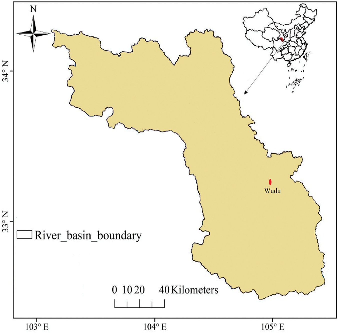
Figure 1: Bailong river catchment

Fig. 2 illustrates the time series variations of streamflow (Q) and sediment load (S) in the Bailong River Basin at Wudu Station. Both streamflow (Q) and sediment load (S) exhibit strong seasonal fluctuations, with high peaks occurring annually. Higher values of Q and S are observed during specific periods, which likely correspond to the monsoon season, where rainfall-induced runoff increases both river discharge and sediment transport. The sediment load (S) follows a similar trend to streamflow (Q), with sharp peaks in sediment concentration occurring concurrently with high streamflow events. This suggests that high-discharge events, likely driven by heavy precipitation, increase erosion and sediment transport. The brief statistical characteristics of the data are provided in Table 1. The sediment load is highly skewed (skewness > 7), the dataset has extremely high-sediment transport events. The standard deviation of sediment load in the test dataset (705.1 kg/s) is significantly higher than in the training dataset (481.9 kg/s), suggesting that the test period contains more variable sediment transport patterns.

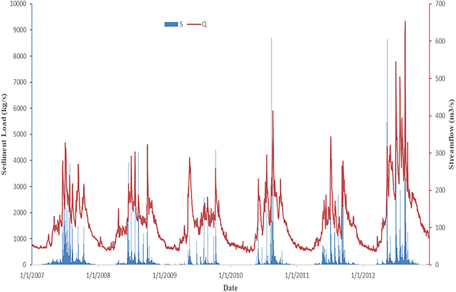
Figure 2: Time series of streamflow (Q) and sediment load (S) at Wudu station

2.2 Methods

This section introduces the methods applied in this study to construct and execute computational tools for modeling the discharge-sediment relationship. The methodology consists of two types of Machine Learning (ML) usages (see Fig. 3), (i) the Multivariate Adaptive Regression Splines (MARS) model for determining the optimal input combination to construct the models (feature selection), and (ii) the regular ANFIS and hybrid (integrative) ANFIS models combined with three meta-heuristic algorithms, namely the PSO, GWO, and GBO, for the sake of simulating the process. In the following, related explanations to each method(ology) are given.

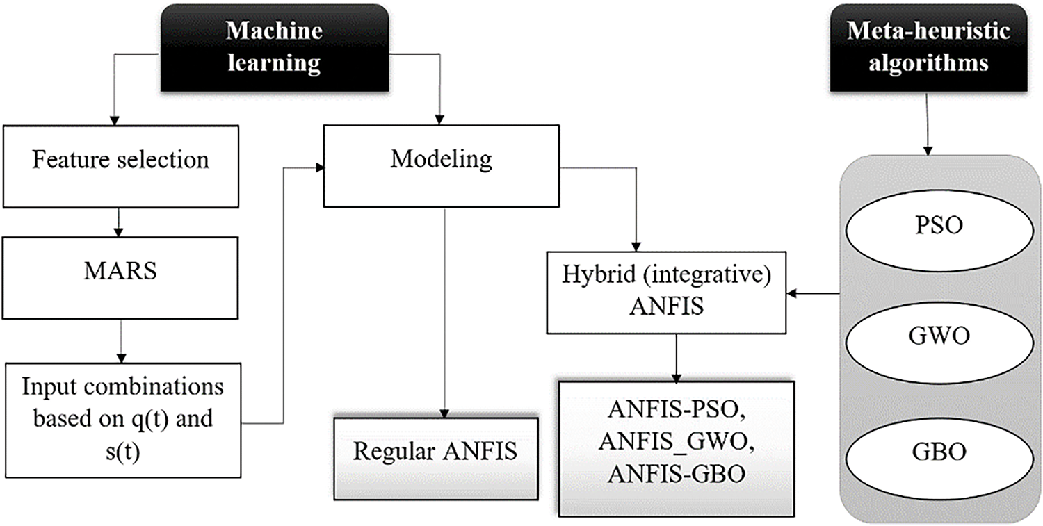
Figure 3: Schematic diagram for the methodology applied in this research

2.2.1 Multivariate Adaptive Regression Splines (MARS)

The MARS method is developed based on a local regression technique that employs a succession of local Basis Functions (BF) to model complicated and nonlinear relationships. The predictor space is divided into several (overlapping) areas where spline functions are fitted. The weighted total of the local models yields the global MARS model based on the following function:

y^=a0+∑m=1MamBm(x)(1)

In relation (1), y^ represents the predicted value, a0 and am stand for the coefficients of the constant bias and mth BF, respectively; and M shows the number of the included BFs in the model. Through a three-step process, the MARS model is able to find the optimal input combination model to be employed in other models for modeling the response parameter (here, s(t)).

•   Step 1: BFs are introduced and added using a stepwise procedure. Then, combined in a weighted sum to construct the model;

•   Step 2: backward elimination procedure for pruning the constructed model;

•   Step 3: Selection of the best (optimized) model.

Detailed information related to the MARS model can be found in Friedman [34], Sekulic et al. [35] and Put et al. [36].

2.2.2 Adaptive Neuro-Fuzzy Inference System (ANFIS)

Among the fuzzy neural network (FNN) models, ANFIS is known as the most frequently used one due to its transparent Fuzzy Inference System (FIS), robustness in outcomes, and moderate computational time [37–39]. ANFIS combines the concepts of a five-layer feedforward artificial neural network with the rules of FIS to reach an adaptive model for adjusting the parameters in its nodes. In order to describe complex nonlinear systems, the ANFIS model divides the input space into many local regions and uses Membership Functions (MFs) to split the input dimension. The splitting process makes the ANFIS model activate several local regions simultaneously for a single input variable. After the initial establishment of the network, a combined two-step learning algorithm is used until it reaches the convergence/termination epoch based on the two forward and backward passes as below:

(a)   Least Squares Estimate (LSE) via a forward pass to adjust the consequent parameters.

(b)   Gradient Descent (GD) method via a backward pass to propagate the errors of the premise parameters.

It is worth mentioning that the premise parameters are referred to as the MFs, and the russification process is executed in layer one. In most cases, bell-shaped functions are used to form the MFs. The consequent parameters are related to the adjustable parameters of the adaptive nodes of linear equations in the Takagi-Sugeno model. More information regarding the ANFIS model and its training process is given in [27].

2.2.3 Particle Swarm Optimization (PSO)

Multiple PSO is a population-based search technique inspired by the collective intelligence of animal movements in groups (e.g., flocks of birds or schools of fish) in which each potential solution, known as a swarm, represents a population particle [40–42]. The particle’s position is changed constantly in a multidimensional search space until the optimal response and/or computational constraints are reached. This algorithm begins by randomly generating an initial population (a group of particles). In reality, each particle demonstrates a potential response. Each particle moves and searches in the problem space for the best possible location. This particle is fitted by its objective function and directed in the most suitable direction at each step to determine the most accurate and precise response. Each particle moves forward using its knowledge and neighbors in the problem search space. Other particles move toward the best-positioned particle and correct their paths.

As a result, the movement of particles in the solution search space is determined by three features: the particle’s current position (Xik), the best location that a particle has encountered (Pbest), and the best location that all of the particles have encountered (Gbest). The prevalent equations for calculating these features are as follows:

{Vi(k+1)=wVik+c1r1.(Pbesti−Xik)+c2r2.(Gbest−Xik)Xi(k)=Xi(k−1)+Vik(2)

where i=1,2,…,N, (N stands for the population size or the number of particles), k represents the iterations number, V is the velocity vector, and X is the particle’s position. c1,c2 are two positive values and r1,r2 are random numbers between null and unity.

In other words, Pbest is a particle’s best prior position. Gbest also symbolizes the best particle among all particles in the swarm. Every particle can record its own personal best position (Pbest) and determine the most suitable positions identified by all particles in the swarm (Gbest). All particles flying over the D-dimensional solution space are exposed to updated rules for new positions until the global optimum position is reached. The accompanying stochastic and deterministic update rules show how a particle’s velocity and location are [43].

2.2.4 Grey Wolf Optimization Method (GWO)

GWO is a nature-inspired advanced meta-heuristic algorithm that can be employed for efficient optimization [44–46]. This algorithm was created by mimicking the foraging behavior of grey wolves, which hunt in groups of five to twelve individuals at the summit of the food chain. Based on the natural behavior of wolf packs, four distinct types of wolves can be distinguished. (i) Alphas (α) who are the leaders that make decisions while hunting, migrating, resting, etc. (ii) Betas (β), assist the alphas in leading the pack. Nonetheless, they must obey the alphas; (iii) the next rank is known as deltas (δ), and they serve the pack as scouts and hunters, assisting α and β wolves in hunting ; (iv) The final stage are the weakest wolves known as omegas (ω) who might participate in some of the pack’s activities. The hunting behavior of wolves is mathematically modeled in three key phases: (i) encircling prey, (ii) hunting, and (iii) attacking prey. These steps are examined in detail in the following:

(i) Encircling Prey

The position of wolves during the encircling phase is updated based on the position of the prey. This is mathematically expressed as:

D→=|C→.X→prey(t)−X→(t)|X→(t+1)=X→prey(t)−A→.D→(3)

where X→prey is the position of the prey, and X→(t) is the position of the current solution at time t. The A→,C→ vectors can be calculated as: A→=2.a→.r→1−a→,C→=2.r→2. Here, r→1,r→2 are random numbers between 0 and 1. Also, a→ is a coefficient vector that decreases linearly from 2 to zero during the iteration process.

(ii) Hunting Process

The top three wolves lead the hunting phase (α, β, and δ). Their positions guide the movement of the pack as follows:

X→(t+1)=X→α+X→β+X→δ3(4)

where X→ vector represents the best solution for each agent so far.

(iii) Attacking Prey

As the wolves close in on the prey, the value of a→ approaches 0, reducing the exploration factor and increasing exploitation. This allows the wolves to fine-tune their positions around the optimal solution.

It should be noted that the parameters α, β, and δ are hierarchical ranks representing the best, second-best, and third-best solutions. α Represents the most optimal solution (leader of the pack), β stands for the second-best solution, which assists α in decision-making, and δ presents the third-best solution, which assists both α and β. More explanations regarding the application of GWO can be found in [46].

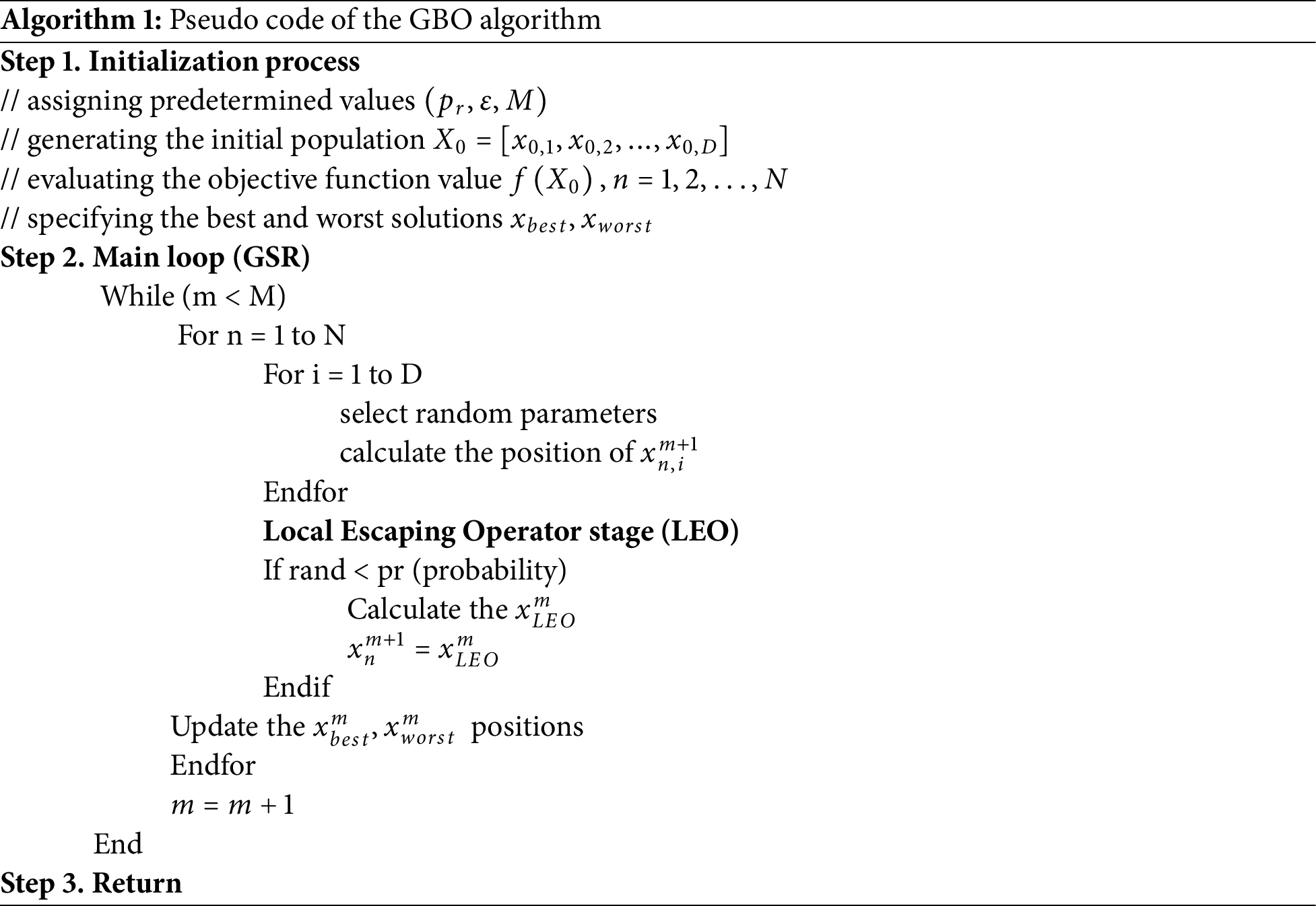
2.2.5 Gradient-Based Optimizer (GBO)

The GBO combines two distinct optimization algorithms, gradient-based and population-based, to solve complicated optimization problems [47,48]. The Newton’s method (viz., a modification of this method) is used in the GBO for formulating the algorithm to search the solving space using vectors and two types of operators, including the gradient search agents and the local escaping ones [32]. The optimization process can be divided into three main steps: (i) initialization, (ii) gradient search rule, and (iii) local escaping operator to update the best solution xbestm at the mth iteration, as follows:

i. The initialization step

The GBO, like most meta-heuristic population-based algorithms, begins the optimization process with an independent population created from a uniform random distribution. Each population agent is referred to as a “vector,” and the population contains N vector agents in a D-dimensional search field. The setup procedure is then carried out as follows:

Xn=Xmin+rand(0,1)×(Xmax−Xmin)(5)

In the above equation, X denotes the decision variable, and rand(0,1) function produces a random number between zero and one.

ii. The gradient search rule step (GSR)

After setting the initial random populations, the movement of vectors is controlled by the gradient search rule (GSR) to achieve a better searching procedure in the feasible domain and obtain improved positions. ρ1, as a substantial factor in balancing the exploration and exploitation processes, is used for this purpose, is calculated as below:

ρ1=2×rand×α−α{α=|β×sin⁡(3π2+sin⁡(β×3π2))|β=βmin+(βmax−βmin)×(1−(mM)3)2,βmin=0.2,βmax=0.8(6)

where m denotes the iteration number and M is the total number of iteration, and α is a factor for adjusting the transition from the exploration to exploitation.

At this stage, the GSR can be determined as:

GSR=randn×ρ1×2Δx×xn(ypn−yqn+ε)(7)

In Eq. (7), ypn,yqn are positions created based on the Gradient Estimation algorithm. Combining the exploration and exploitation phases, the current position of the searching agent (Xnm) can be updated according to the following relation:

xnm+1=ra×(rb×X1nm+(1−rb)×X2nm)+(1−ra)×X3nmX3nm=Xnm−ρ1×(X2nm−X1nm)(8)

where ra and ra are random numbers between zero and one.

iii. The local escaping operator (LEO)

To improve the performance of an optimization algorithm for solving complex problems, the Local Escaping Operator (LEO) is developed. The LEO can efficiently update the solution’s position. As a result, it helps an algorithm get out of local optima spots and accelerates convergence. The LEO employs targets to create a novel solution that outperforms the competition as the xLEOm. Combining the three main steps, the pseudo code for the GBO algorithm as shown below (Algorithm 1). The pseudo code of ANFIS-GBO is reported here.

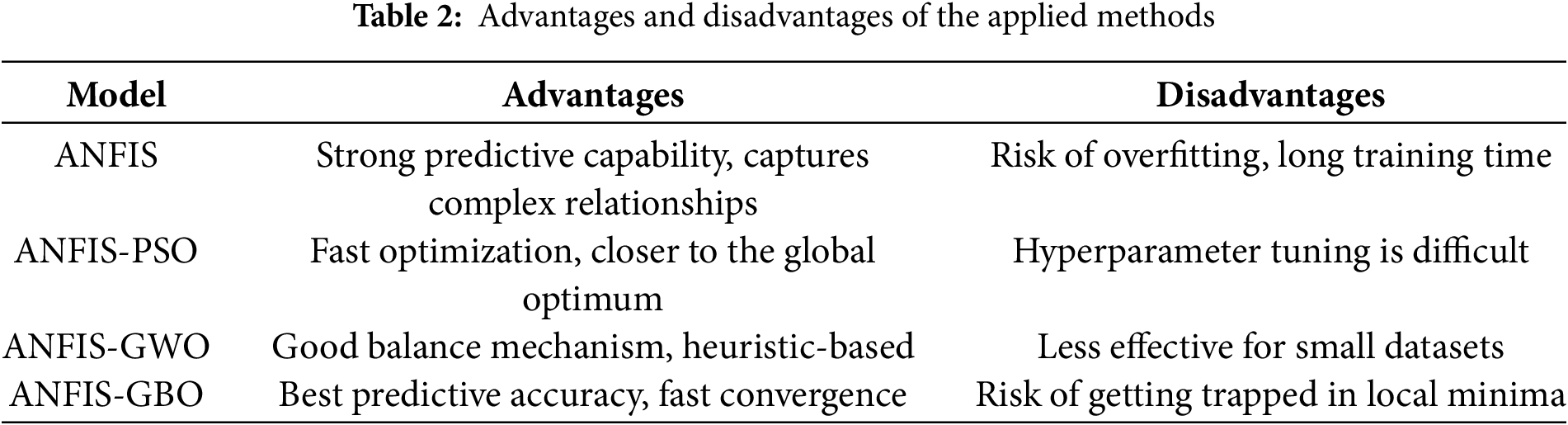
2.2.6 Hybrid ANFIS Models: Fundamentals and Comparison

The standard ANFIS model combines the strengths of fuzzy logic and neural networks to model complex nonlinear relationships. However, its performance is often limited by parameter tuning and convergence behavior challenges. To overcome these limitations, our study incorporates three optimization techniques, namely (i) ANFIS-PSO, (ii) ANFIS-GWO, and (3) ANFIS-GBO. The ANFIS-PSO model integrates PSO into the ANFIS framework. PSO optimizes the ANFIS parameters by updating a swarm of candidate solutions through velocity and position adjustments based on individual best (Pbest) and global best (Gbest) positions. This iterative search process enhances the model’s ability to efficiently explore the parameter space and converge to an optimal solution. In the ANFIS-GWO model, the GWO algorithm is employed. GWO simulates the social hierarchy and hunting mechanism of grey wolves, where the top three solutions (alpha, beta, and delta) guide the search process. This approach effectively balances exploration and exploitation, enabling the model to navigate complex solution landscapes and avoid local optima. The ANFIS-GBO model incorporates the GBO, a novel algorithm that merges gradient-based search with population-based strategies. GBO utilizes a gradient search rule to accelerate convergence and a local escaping operator to prevent premature convergence to suboptimal solutions. This dual mechanism ensures a robust and efficient tuning of the ANFIS parameters.

This section also provides a comparative analysis of the principles, advantages, and limitations of the applied methods. Table 2 summarizes the strengths and weaknesses of different ANFIS-based models combined with optimization algorithms.

2.3 Accuracy Assessment

The viability of three hybrid ANFIS methods, ANFIS-PSO, ANFIS-GWO and ANFIS-GBO, was evaluated in predicting daily suspended sediment load (SSL). The models were assessed using data from the Bailong River Basin and three commonly employed statistical indices. The methods were also visually assessed using scatterplots, Taylor and violin charts. The statistical indices can be expressed as:

RMSE=1N∑i=1N[(SSL0)i−(SSLC)i]2(9)

MAE=1N∑i=1N|(SSL0)i−(SSLC)i|(10)

R2=[∑i=1N((SSL0)i−(SSL0¯)i)((SSLC)i−(SSLC¯)i)∑i=1N((SSL0)i−(SSL0¯)i)2((SSLC)i−(SSLC¯)i)2]2(11)

where SSL0, SSLC, SSL0¯, N are observed, computed, mean of the observed daily SSL and data quantity, respectively. Various input combinations of streamflow (Q) and SSL data were considered inputs to the ANFIS-based models.

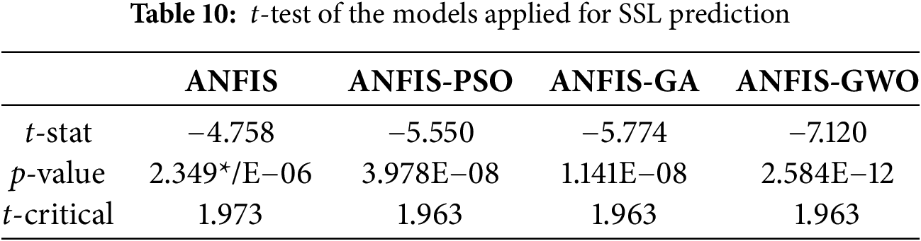
To statistically assess the efficiency of the proposed models, we performed a paired t-test to compare the mean prediction errors of different ANFIS-based models. The t-test examines whether the differences between models are statistically significant, using a confidence level of 95% (α = 0.05). A model with a t-statistic greater than the critical value and p-value below 0.05 indicates a significant performance improvement over the baseline (ANFIS).

3  Results

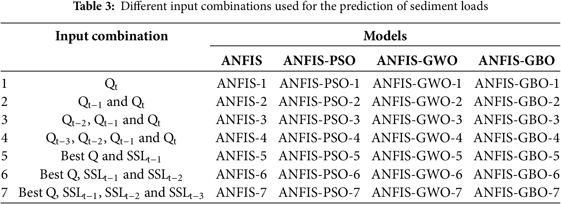
This section reports the results of all utilized models for predicting suspended sediment load daily. Table 3 lists the input combinations and names of the corresponding models. In the table, Qt−1 and SSLt−1 refer to the streamflow and SSL values of one previous day and vice versa. In the first four combinations, only streamflow data were considered inputs and then the lagged SSL data were added to the Q-based inputs obtained from the first four. Data covering the period from 01 January 2007 to 30 June 2011 (75% of the whole data) were used for the training stage, and data from 01 July 2011 to 31 December 2012 (25% of the whole data) were used for the testing stage. One hundred iterations were applied for all ANFIS-based models. Before applying ANFIS-based methods, MARS method was applied to the input combinations provided in Table 3 to decide the best input scenario. The rationale behind selecting these different input combinations was to systematically assess the impact of lagged streamflow and SSL data on model performance. We progressively added lagged values to capture temporal dependencies and identify the optimal balance between model complexity and predictive accuracy. This step was crucial in understanding how past observations influence SSL predictions and determining whether increasing the number of inputs would improve model performance or lead to redundancy and overfitting.

The MARS method has a simpler structure and is much easier to apply compared to ANFIS-based methods. Therefore, we evaluated whether the MARS method could effectively determine the best input combination for daily SSL prediction before applying more complex models. Table 4 summarizes the training and test outcomes of the MARS models for seven different input scenarios. The results indicate a clear trend: the MARS model’s accuracy improves in both the training and test stages as the number of input variables increases from Scenario 1 to Scenario 7, except for Scenario 4, which exhibits slightly worse performance than Scenario 3. This decline in accuracy could be attributed to the redundancy or noise introduced by additional input variables that do not contribute significantly to the model’s predictive capability. This phenomenon, often called the “curse of dimensionality,” suggests that including too many variables without proper feature selection can negatively impact model performance by increasing variance without substantial gains in accuracy.

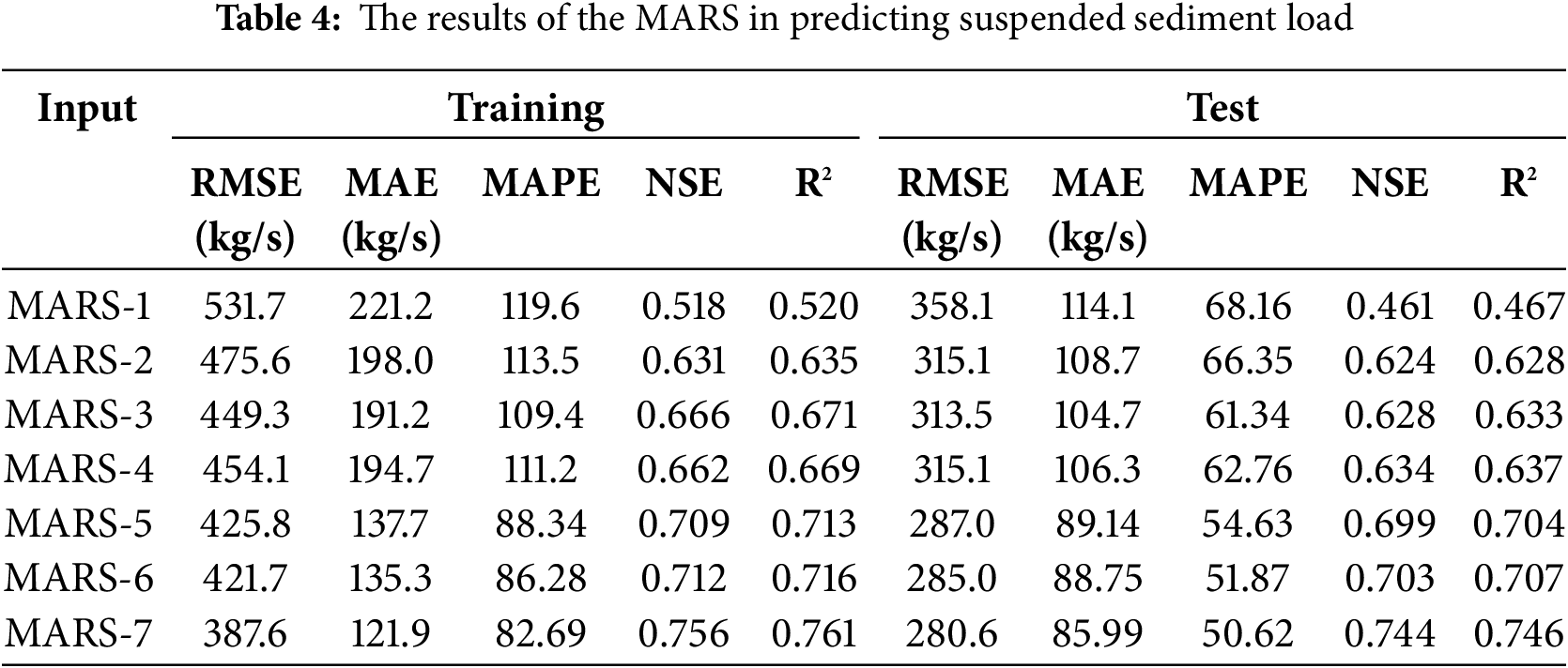
The best predictive accuracy was obtained from the MARS model using the full set of input variables, achieving the lowest RMSE (387.6 kg/s), MAE (121.9 kg/s), and MAPE (82.69), along with the highest NSE (0.756) and R2 (0.746) in the test stage. These results highlight the potential of MARS as a preliminary feature selection tool capable of identifying optimal input combinations before applying more sophisticated machine learning models. However, since MARS is a piecewise regression-based approach, it may not fully capture the nonlinear and dynamic relationships inherent in suspended sediment transport processes. Therefore, to further enhance predictive performance, we proceed with applying standard ANFIS and three hybrid ANFIS-based methods (ANFIS-PSO, ANFIS-GWO, and ANFIS-GBO) to the same input combinations, ensuring a more comprehensive evaluation of model effectiveness in daily SSL prediction.

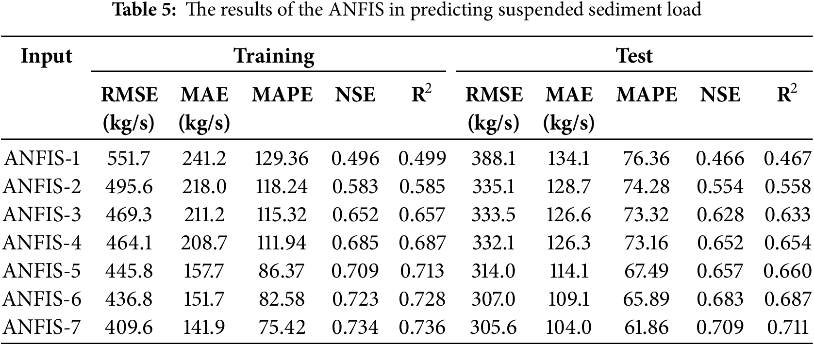
Training and testing outcomes of the standard ANFIS models are given in Table 5 for SSL prediction. As observed from the table, increasing input number improves the prediction accuracy of the method; RMSE, MAE, MAPE, NSE and R2 range from 388.1 kg/s, 134.1 kg/s, 76.36, 0.466 and 0.467 to 305.6 kg/s, 104 kg/s, 61.86, 0.709 and 0.711, respectively. The last input combination offered the best accuracy in predicting SSL for the training and testing stages. Considering previous SSL data as inputs improves the RMSE, MAPE, MAE, NSE and R2 by 8%, 17.7%, 15.4, 8.7% and 8.7% in the test stage, respectively (compare the input cases 4 and 7). These improvements highlight the importance of capturing temporal dependencies in sediment load prediction. The historical SSL data likely contribute crucial contextual information about sediment behavior, particularly during peak events and extreme conditions.

Tables 6–8 illustrate the training and testing results of the hybrid ANFIS method, including ANFIS-PSO, ANFIS-GWO and ANFIS-GBO in predicting daily SSL. It is apparent from the tables that the accuracy of the models is improved by importing more inputs in all models and for both the training and testing stages. The RMSE, MAE, MAPE, NSE and R2 range from 376.3 kg/s, 124.7 kg/s, 71.43, 0.502 and 0.505 to 270.2 kg/s, 71.4 kg/s, 47.31, 0.743 and 0.747 for ANFIS-PSO while the corresponding ranges are 366.6–228.3 kg/s, 115.8–63.8 kg/s, 67.21–43.72, 0.531–0.766 and 0.537–0.769 for ANFIS-GWO and 355.6–207.2 kg/s, 111.8–47.5 kg/s, 64.25–36.65, 0.549–0.816 and 0.554–0.822 for ANFIS-GBO in the test stage, respectively.

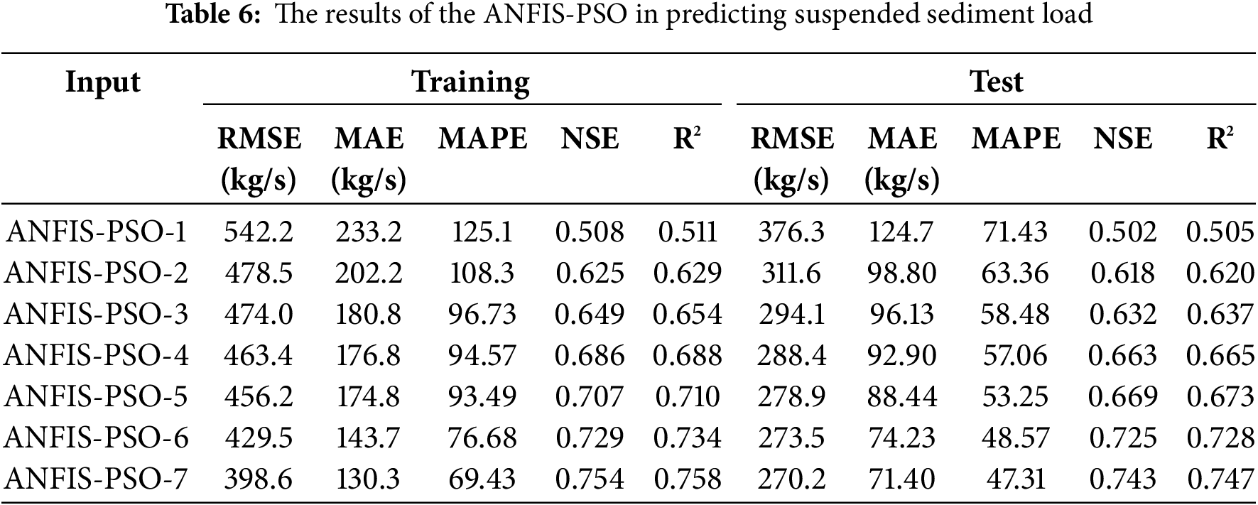
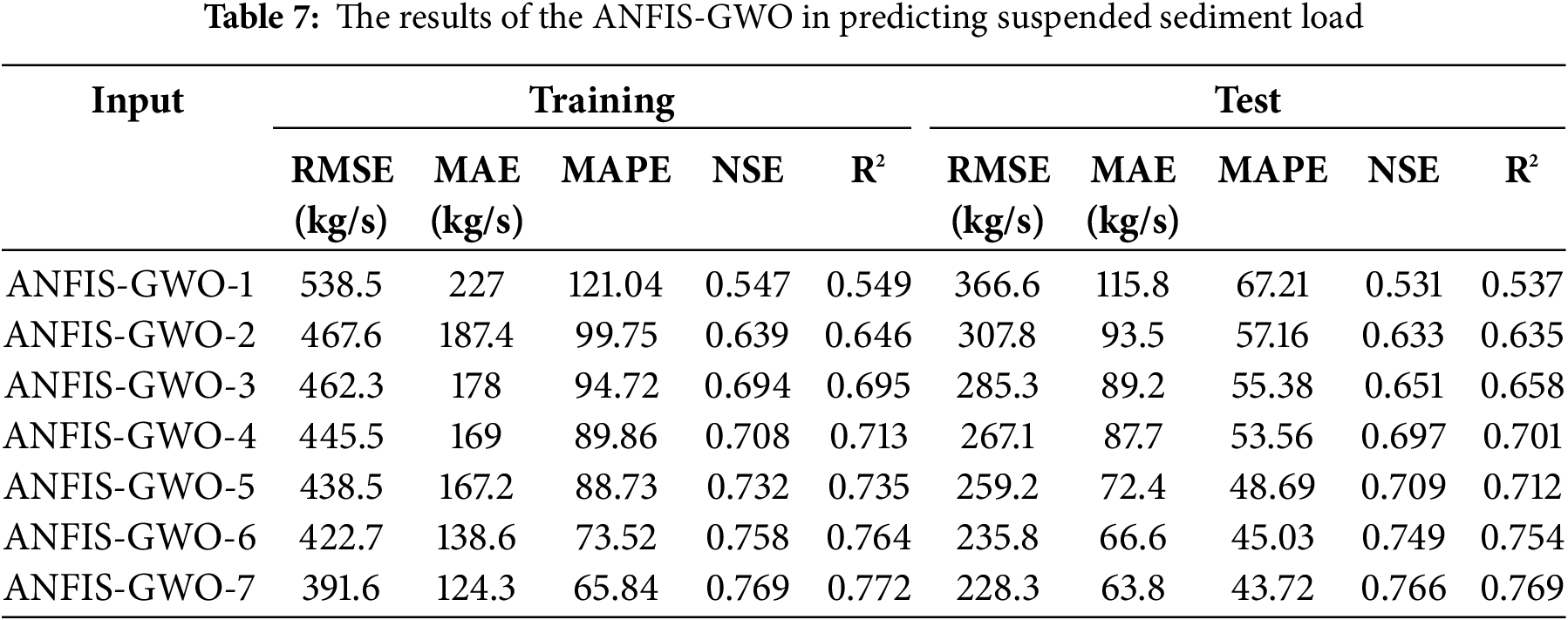
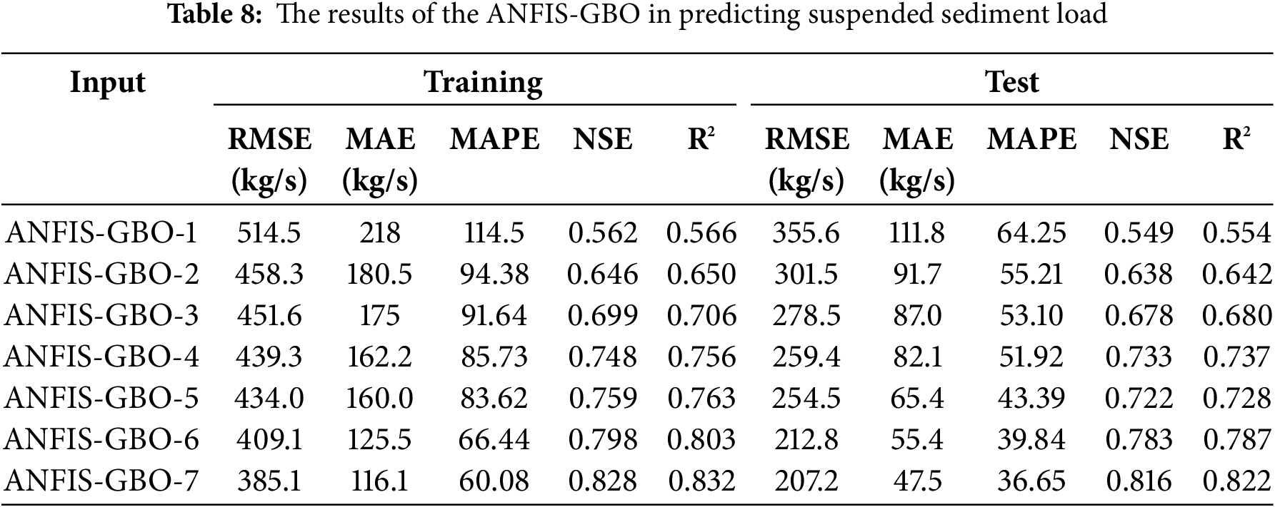
It is understood from the ranges that the hybrid methods considerably improve the prediction accuracy of the standard ANFIS; the RMSE and MAE of the best ANFIS are improved by 11.6% and 31.3%, 25.3% and 38.7%, 32.2% and 54.3% applying ANFIS-PSO, ANFIS-GWO and ANFIS-GBO in the test stage, respectively. Among the hybrid approaches, the ANFIS-GBO acted as the best model with the lowest RMSE (207.2 kg/s), MAE (47.5 kg/s), MAPE (36.65) and the highest NSE (0.816) and R2 (0.822) in daily SSL prediction.

Notably, the consistent improvement across all hybrid models highlights the effectiveness of metaheuristic optimization in refining ANFIS parameters and enhancing model learning. The significant reduction in RMSE and MAE further confirms that these optimization techniques effectively mitigate the limitations of standard ANFIS, such as slow convergence and sensitivity to local minima. It should be noted that the model’s performance is improved by taking into account the previous SSL data as inputs; improvements in testing RMSE are 6.3%, 14.5% and 20.1% for ANFIS-PSO, ANFIS-GWO and ANFIS-GBO (compare the inputs scenarios 4 and 7), respectively. This result suggests that incorporating historical SSL values allows the models to better capture temporal dependencies and sediment transport patterns, particularly in high-fluctuation conditions.

A statistical comparison of the models reveals that while ANFIS provides a robust baseline, including metaheuristic optimization, it significantly enhances its predictive capabilities. Among the hybrid methods, ANFIS-GBO demonstrated superior performance, likely due to its efficient gradient-based search mechanism, which optimally tunes ANFIS parameters while avoiding local minima. The improvement in RMSE and MAE of ANFIS-GBO over standard ANFIS was 32.2% and 54.3%, respectively, highlighting the effectiveness of the optimization approach. These findings emphasize the potential of ANFIS-GBO as a reliable tool for SSL prediction, particularly in complex hydrological systems where conventional models struggle to generalize. Future research should explore additional input features and optimization techniques to refine model accuracy.

Table 9 compares the hybrid ANFIS methods for catching peak sediment loads during the testing stage. The threshold value is 2000 kg/s and there are 18 peaks in the data. The total absolute relative errors clearly show that the ANFIS-GBO offered the best accuracy by providing the lowest error (1010.6).

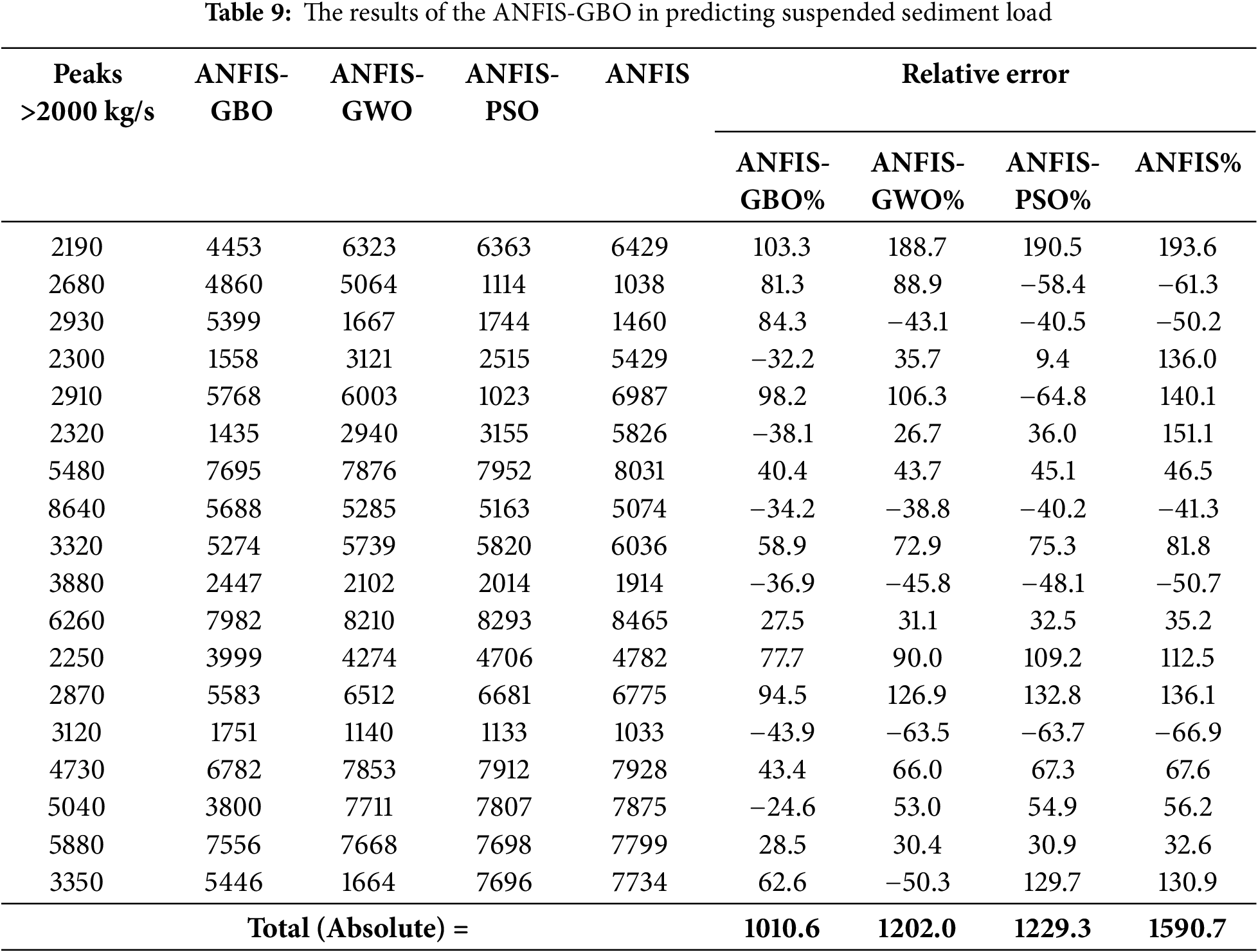
Furthermore, the results confirm that metaheuristic optimization significantly enhances the ability of ANFIS to predict extreme sediment transport events, which are often challenging due to their irregularity and high variability. The improvements in peak estimation accuracy are notable, with reductions in error of 36.5%, 24.4%, and 22.7% when applying GBO, GWO, and PSO, respectively. This suggests that ANFIS-GBO effectively balances exploration and exploitation in its search space, leading to improved parameter tuning and better adaptation to peak sediment fluctuations.

Capturing peak sediment loads is crucial in hydrological modeling, as extreme sediment transport events can significantly impact river morphology, reservoir sedimentation, and flood risk management. The superior performance of ANFIS-GBO in this aspect highlights its potential as a robust tool for predicting high-impact sediment transport events with improved reliability. Future studies should investigate its applicability to different river basins and extreme hydrological conditions.

The bar plot in Fig. 4 presents the average RMSE, MAE, and MAPE for different ANFIS-based models in predicting suspended sediment load (SSL) during the test period. ANFIS-GBO outperforms all other models, showing the lowest RMSE, MAE, and MAPE among the four models. ANFIS, the standard model, has the highest errors, indicating that optimization significantly improves prediction performance. Hybrid models (ANFIS-PSO, ANFIS-GWO, and ANFIS-GBO) reduce errors, but ANFIS-GBO provides the most significant improvement. Error metrics follow a decreasing trend as optimization algorithms are applied. The findings emphasize the importance of metaheuristic algorithms in improving hydrological predictions.

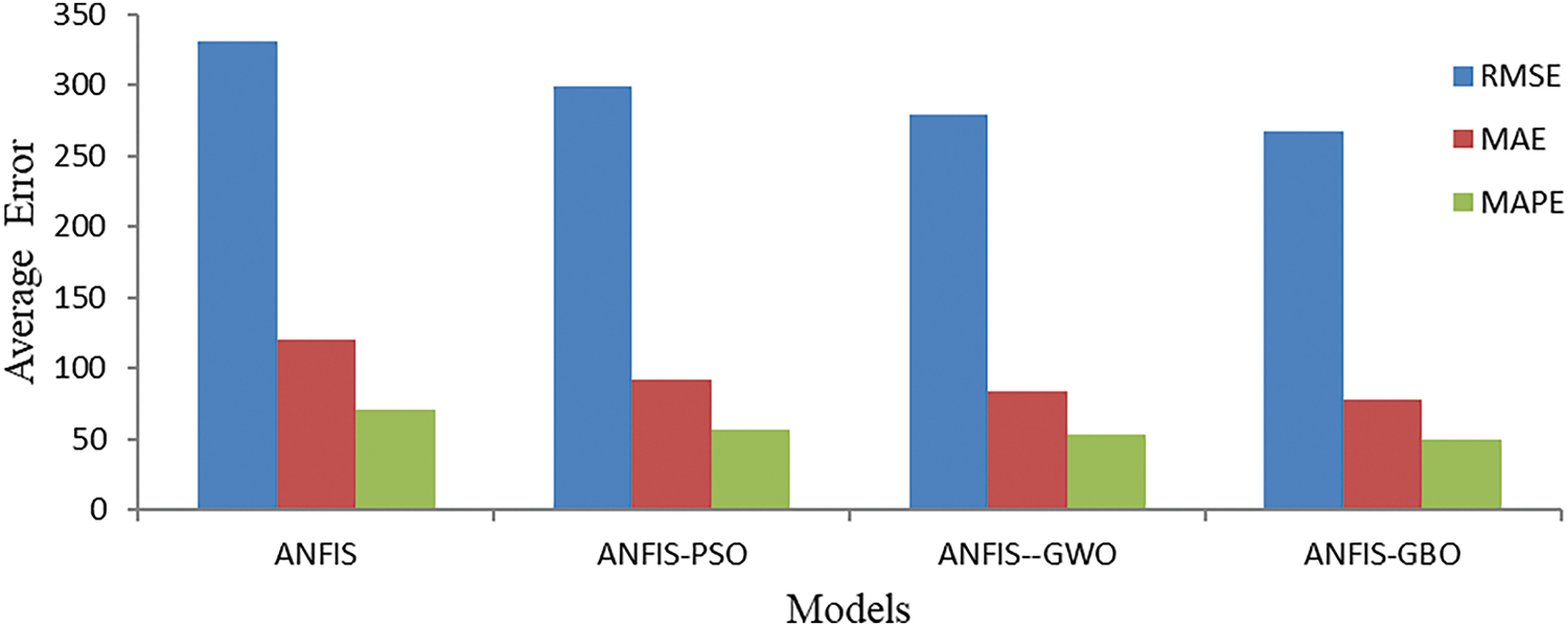
Figure 4: Average RMSE, MAE and MAPE of the applied models in predicting SSL using different ANFIS based models during the test period

Fig. 5 illustrates the scatterplots depicting the comparison between the observed and predicted suspended sediment loads during the test period. The scatter graphs indicate that the ANFIS-GBO model exhibits less scattered predictions compared to the other models. To assess the ANFIS-based models comprehensively, Fig. 6 presents a Taylor Diagram, which provides a statistical comparison of the applied models (ANFIS, ANFIS-PSO, ANFIS-GWO, and ANFIS-GBO) for suspended sediment load (SSL) prediction. The diagram evaluates model performance using three key statistical metrics: standard deviation, correlation coefficient (r), and Root Mean Square Error (RMSE). The standard deviation, represented along both axes, indicates the spread of predictions compared to the observed dataset (red dot). The curved green lines represent RMSE values, where models positioned closer to the observed point exhibit lower prediction errors. The blue radial lines indicate the correlation coefficient, showing the strength of agreement between the model predictions and actual observations. A model with a higher correlation, lower RMSE, and a standard deviation similar to the observed data is considered more accurate. As illustrated in Fig. 5, the ANFIS-GBO model (green point) demonstrates a higher correlation and lower RMSE compared to other models, indicating its superior performance in SSL prediction. Conversely, the ANFIS model (yellow point) exhibits relatively lower accuracy, highlighting the effectiveness of optimization techniques in improving predictive performance.

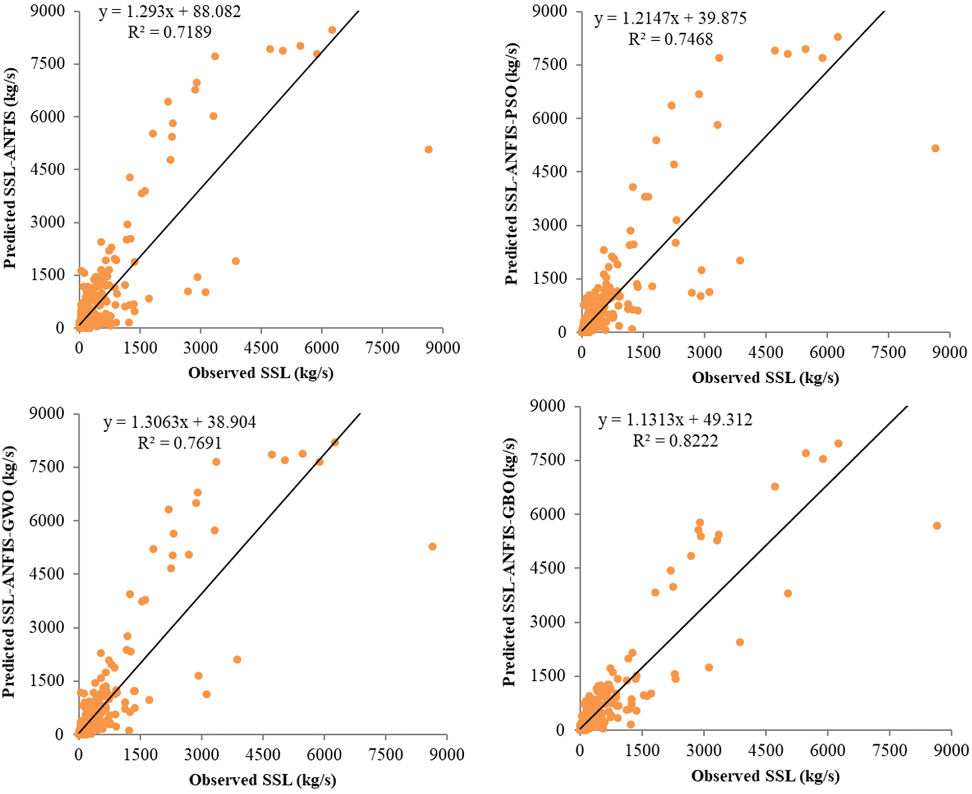
Figure 5: Scatterplots of the observed and predicted SSL by different ANFIS based models during the test period using the best input combination (input combination 7)

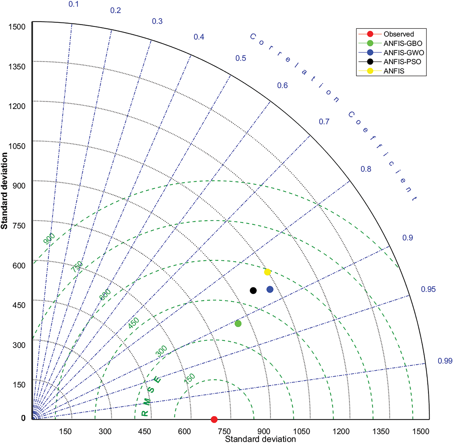
Figure 6: Taylor Diagram comparing the performance of the ANFIS, ANFIS-PSO, ANFIS-GWO, and ANFIS-GBO models for SSL prediction. The red dot represents the observed data, while the model predictions are color-coded. Models closer to the observed point, with higher correlation coefficients and lower RMSE, demonstrate better predictive performance

Fig. 7 presents a violin plot comparing the distribution of measured and predicted suspended sediment load (SSL) values across different models, including ANFIS, ANFIS-PSO, ANFIS-GWO, and ANFIS-GBO. The x-axis represents the different models and the observed (measured) values, while the y-axis indicates the SSL values in kg/s. The shape of each violin plot illustrates the probability density of SSL predictions, where wider sections indicate a higher frequency of values, and narrower sections indicate a lower frequency. The red boxplots within each violin highlight the interquartile range (IQR) and median values of SSL predictions. The measured data (first violin) provides a reference distribution, against which the models’ predictive accuracy is assessed. Among the predictive models, ANFIS-GBO exhibits a more consistent and concentrated distribution around the measured SSL values, suggesting improved prediction stability and reduced variance. The baseline ANFIS model shows a broader spread, indicating greater prediction variability. These results reinforce the effectiveness of metaheuristic optimization techniques in refining ANFIS-based models for SSL prediction, with ANFIS-GBO achieving the most reliable predictive performance.

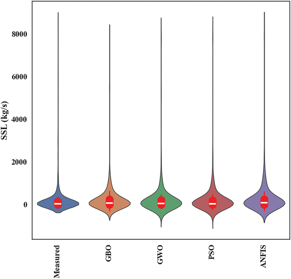
Figure 7: Violin plot showing the distribution of measured and predicted SSL values for different models having the best input combination. The red boxplots indicate the interquartile range (IQR), while the width of each violin plot represents the probability density of SSL predictions. A narrower distribution closer to the measured data suggests higher predictive accuracy

4  Discussion

The feasibility of a new hybrid ANFIS-GBO was investigated and compared with standard ANFIS and two hybrid ANFIS methods (ANFIS-PSO and ANFIS-GWO) in predicting daily SSL. The results showed that incorporating more input variables generally improved the prediction accuracy of all models. Adding SSL data from previous days as inputs had a particularly positive impact on the models’ performance. This indicates that historical SSL data contains valuable information for predicting future SSL values. The improvement in prediction accuracy, as measured by RMSE, MAE, and R2, highlighted the importance of considering temporal dependencies in the SSL prediction task. On the other hand, adding streamflow data to the MARS model inputs resulted in a degradation of prediction accuracy, as evident from Table 4. This observation aligns with previous studies conducted by researchers such as Adnan et al. [49], Sharafati et al. [50] and Rahgoshay et al. [51]. These studies have consistently reported that an increase in the number of inputs does not necessarily lead to improved prediction accuracy and can have a negative impact on variance. Consequently, this may result in more complex models with poorer prediction performance. For instance, Adnan et al. [49] compared machine learning methods for predicting river flow. They found that including precipitation data as an input did not enhance the accuracy of the models.

Adding SSL data from previous days as inputs had a particularly positive impact on the models’ performance. This indicates that historical SSL data contains valuable information for predicting future SSL values. The improvement in prediction accuracy, as measured by RMSE, MAE, and R2, highlighted the importance of considering temporal dependencies in the SSL prediction task. On the other hand, it was found from the models’ outcomes that only streamflow-based input scenarios also provided acceptable accuracy in SSL prediction. As Tao et al. [52] discussed, a crucial concern in modeling SSL is the common reliance on previous SSL values as model inputs. However, this approach poses practical challenges due to the difficulty in accurately measuring SSL data, particularly during extreme events. Alternatively, emphasizing water level data alone, rather than streamflow, holds greater significance in SSL modeling. This is especially pertinent for developing countries where essential variables may be unavailable or lacking at many monitoring stations. By prioritizing water level data, the limitations associated with SSL measurements can be mitigated, facilitating more feasible and effective SSL modeling approaches.

Comparing the different modeling approaches, the hybrid ANFIS methods (ANFIS-PSO, ANFIS-GWO, and ANFIS-GBO) consistently outperformed the standard ANFIS model in terms of prediction accuracy. Among the hybrid methods, ANFIS-GBO emerged as the best-performing model, achieving the lowest RMSE, MAE, MAPE, NSE and the highest R2 in daily SSL prediction. This indicates that the combination of ANFIS with the GBO optimization algorithm led to superior performance in capturing the complex relationships between input variables and SSL. The considerable improvements in prediction accuracy obtained by the hybrid ANFIS methods highlighted the effectiveness of using nature-inspired optimization algorithms (PSO, GWO, and GBO) to enhance the learning and adaptation capabilities of the ANFIS model. These algorithms enabled the models to search the solution space more effectively and find better parameter configurations, leading to improved predictions.

While the evaluation metrics (RMSE, MAE, MAPE, NSE and R2) demonstrate the improved performance of ANFIS-GBO compared to other models, statistical validation is necessary to confirm the significance of these improvements. Table 10 presents the results of the paired t-test, comparing the performance of each model against ANFIS. The results indicate that all optimization-based ANFIS models significantly outperform standard ANFIS (p < 0.05). ANFIS-GWO exhibited the highest statistical significance (t = −7.120, p = 2.584E−12), confirming its superior predictive ability. The negative t-values suggest that the optimized models have lower mean prediction errors than the baseline ANFIS model. These results validate the effectiveness of using metaheuristic optimization techniques in SSL modeling, with ANFIS-GBO providing the most stable and accurate predictions.

Overall, the study demonstrated the effectiveness of ANFIS-based models, especially the hybrid approaches, in predicting daily suspended sediment load in the Bailong River Basin. Incorporating historical SSL data and utilizing nature-inspired optimization algorithms significantly improved the models’ performance. As shown in Table 8, ANFIS-GBO achieved the highest accuracy with the lowest RMSE and MAE due to its efficient optimization process and reduced computational cost. Compared to other models, ANFIS-GBO required fewer control parameters while maintaining a robust prediction capability. These findings have implications for water resource management and environmental planning, as accurate prediction of SSL can aid in assessing and mitigating the impacts of sediment transport on river systems and associated ecosystems.

5  Conclusions

This study evaluated the effectiveness of hybrid Adaptive Neuro-Fuzzy Inference System (ANFIS) models integrated with different optimization techniques—Particle Swarm Optimization (PSO), Grey Wolf Optimization (GWO), and the Gradient-Based Optimizer (GBO)—for predicting daily suspended sediment load (SSL). The findings demonstrated that hybrid models significantly improved predictive accuracy compared to the standard ANFIS model. The key conclusions of this study are summarized as follows:

–   Among the tested models, the ANFIS-GBO method achieved the highest prediction accuracy, with the lowest RMSE (207.2 kg/s), MAE (47.5 kg/s), and MAPE (36.65) and the highest NSE (0.816) and R2 (0.822), confirming its capability to effectively model the nonlinear and dynamic behavior of SSL.

–   Including lagged SSL values as inputs significantly enhanced model performance, highlighting the importance of considering temporal dependencies in SSL forecasting. Models incorporating past SSL values consistently outperformed those using only streamflow data.

–   The integration of metaheuristic optimization algorithms (PSO, GWO, and GBO) improved the performance of ANFIS by optimizing parameter selection and preventing local minima trapping. Among these, GBO exhibited the best balance between exploration and exploitation, resulting in faster convergence and more accurate predictions.

–   The Multivariate Adaptive Regression Splines (MARS) method effectively identified the best input combinations, reducing computational complexity while maintaining high accuracy.

–   ANFIS-GBO provided the most reliable predictions for extreme sediment transport events, reducing total absolute relative error by 36.5% compared to the standard ANFIS model.

–   The study underscores the potential of hybrid AI-based approaches in hydrology, demonstrating that nature-inspired optimization can significantly enhance model adaptability to complex environmental conditions.

However, despite the promising results, this study has some limitations. The reliance on historical SSL data may pose practical challenges due to the difficulty in measuring SSL accurately, particularly during extreme weather events. Additionally, the study was conducted on a single river basin, and further validation is required to assess the generalizability of the proposed approach to different hydrological conditions.

To further improve SSL prediction accuracy, future studies should:

–   Incorporate additional environmental and climatic variables such as rainfall, temperature, and land-use characteristics.

–   Investigate the generalizability of the ANFIS-GBO model across different river basins and hydrological conditions.

–   Explore the integration of explainable AI techniques (e.g., SHAP analysis) to enhance model interpretability.

–   Compare ANFIS-GBO with deep learning approaches, such as LSTM (Long Short-Term Memory or transformers, to evaluate potential performance gains.

Overall, this study contributes to advancing AI-driven hydrological modeling and provides a strong foundation for further research in sediment transport prediction.

Acknowledgement: Not applicable.

Funding Statement: This work was supported by the National Natural Science Foundation of China (52350410465), and the General Projects of Guangdong Natural Science Research Projects (2023A1515011520).

Author Contributions: Conceptualization: Rana Muhammad Adnan and Ozgur Kisi; formal analysis: Rana Muhammad Adnan; validation: Ozgur Kisi, Mo Wang, Adil Masood, Mohammad Zounemat-Kermani, Shamsuddin Shahid and Rana Muhammad Adnan; supervision: Ozgur Kisi and Mo Wang; writing—original draft: Ozgur Kisi, Adil Masood, Mohammad Zounemat-Kermani, Shamsuddin Shahid and Rana Muhammad Adnan; visualization: Rana Muhammad Adnan and Adil Masood; investigation: Ozgur Kisi, Mohammad Zounemat-Kermani and Adil Masood. All authors reviewed the results and approved the final version of the manuscript.

Availability of Data and Materials: The data presented in this study will be available on an interesting request from the corresponding author.

Ethics Approval: Not applicable.

Conflicts of Interest: The authors declare no conflicts of interest to report regarding the present study.

References

1. Kisi O. Modeling discharge-suspended sediment relationship using least square support vector machine. J Hydrol. 2012;456(4):110–20. doi:10.1016/j.jhydrol.2012.06.019. [Google Scholar] [CrossRef]

2. Hussan W, Khurram Shahzad M, Seidel F, Nestmann F. Application of soft computing models with input vectors of snow cover area in addition to hydro-climatic data to predict the sediment loads. Water. 2020;12(5):1481. doi:10.3390/w12051481. [Google Scholar] [CrossRef]

3. Abda Z, Zerouali B, Alqurashi M, Chettih M, Santos CAG, Hussein EE. Suspended sediment load simulation during flood events using intelligent systems: a case study on semiarid regions of Mediterranean basin. Water. 2021;13(24):3539. doi:10.3390/w13243539. [Google Scholar] [CrossRef]

4. Ali Khan MY. Regional ANN model for estimating missing daily suspended sediment load in complex, heterogeneous catchments. J Geochem Explor. 2025;269(11):107643. doi:10.1016/j.gexplo.2024.107643. [Google Scholar] [CrossRef]

5. Singh N, Khan MYA. ANN modeling of the complex discharge-sediment concentration relationship in Bhagirathi river basin of the Himalaya. Sustain Water Resour Manag. 2020;6(3):36. doi:10.1007/s40899-020-00396-6. [Google Scholar] [CrossRef]

6. Noori R, Ghiasi B, Salehi S, Esmaeili Bidhendi M, Raeisi A, Partani S, et al. An efficient data driven-based model for prediction of the total sediment load in rivers. Hydrology. 2022;9(2):36. doi:10.3390/hydrology9020036. [Google Scholar] [CrossRef]

7. Khan MYA, Hasan F, Tian F. Estimation of suspended sediment load using three neural network algorithms in Ramganga River catchment of Ganga Basin. India Sustain Water Resour Manag. 2019;5(3):1115–31. doi:10.1007/s40899-018-0288-7. [Google Scholar] [CrossRef]

8. Khosravi K, Golkarian A, Melesse AM, Deo RC. Suspended sediment load modeling using advanced hybrid rotation forest based elastic network approach. J Hydrol. 2022;610(3):127963. doi:10.1016/j.jhydrol.2022.127963. [Google Scholar] [CrossRef]

9. Gupta D, Hazarika BB, Berlin M. Wavelet kernel large margin distribution machine-based regression for modelling the river suspended sediment load. Comput Electr Eng. 2024;120(6):109783. doi:10.1016/j.compeleceng.2024.109783. [Google Scholar] [CrossRef]

10. Samantaray S, Sahoo A, Satapathy DP, Oudah AY, Yaseen ZM. Suspended sediment load prediction using sparrow search algorithm-based support vector machine model. Sci Rep. 2024;14(1):12889. doi:10.1038/s41598-024-63490-1. [Google Scholar] [PubMed] [CrossRef]

11. Samantaray S, Sahoo A. Prediction of suspended sediment concentration using hybrid SVM-WOA approaches. Geocarto Int. 2022;37(19):5609–35. doi:10.1080/10106049.2021.1920638. [Google Scholar] [CrossRef]

12. Tulla PS, Kumar P, Vishwakarma DK, Kumar R, Kuriqi A, Kushwaha NL, et al. Daily suspended sediment yield estimation using soft-computing algorithms for hilly watersheds in a data-scarce situation: a case study of Bino watershed. Uttarakhand Theor Appl Climatol. 2024;155(5):4023–47. doi:10.1007/s00704-024-04862-5. [Google Scholar] [CrossRef]

13. Shabani M, Fathian H, Ali Asadi M, Hosseini M. Predicting daily suspended sediment load in rivers using hybrid and deep learning models-case study: kharestan watershed. Iran J Sci Technol Trans Civ Eng. 2024;48(6):4673–85. doi:10.1007/s40996-024-01447-0. [Google Scholar] [CrossRef]

14. Zhou Y, Yue D, Li S, Liang G, Chao Z, Zhao Y, et al. Ecosystem health assessment in debris flow-prone areas: a case study of Bailong River Basin in China. J Clean Prod. 2022;357(5):131887. doi:10.1016/j.jclepro.2022.131887. [Google Scholar] [CrossRef]

15. Kumar M, Kumar P, Kumar A, Elbeltagi A, Kuriqi A. Modeling stage-discharge-sediment using support vector machine and artificial neural network coupled with wavelet transform. Appl Water Sci. 2022;12(5):87. doi:10.1007/s13201-022-01621-7. [Google Scholar] [CrossRef]

16. Zhao Y, Meng X, Qi T, Chen G, Li Y, Yue D, et al. Estimating the daily rainfall thresholds of regional debris flows in the Bailong River Basin, China. Bull Eng Geol Environ. 2023;82(2):46. doi:10.1007/s10064-023-03068-9. [Google Scholar] [CrossRef]

17. Latif SD, Chong KL, Ahmed AN, Huang YF, Sherif M, El-Shafie A. Sediment load prediction in Johor river: deep learning versus machine learning models. Appl Water Sci. 2023;13(3):79. doi:10.1007/s13201-023-01874-w. [Google Scholar] [CrossRef]

18. Heddam S, Naghibi A, Khosravi K, Singh SK. Suspended sediment load prediction and tree-based algorithms. In: Remote sensing of soil and land surface processes. Amsterdam, The Netherlands: Elsevier; 2024. p. 257–69. [Google Scholar]

19. Sahoo BB, Sankalp S, Kisi O. A novel smoothing-based deep learning time-series approach for daily suspended sediment load prediction. Water Resour Manag. 2023;37(11):4271–92. doi:10.1007/s11269-023-03552-7. [Google Scholar] [CrossRef]

20. Rezaei K, Pradhan B, Vadiati M, Nadiri AA. Suspended sediment load prediction using artificial intelligence techniques: comparison between four state-of-the-art artificial neural network techniques. Arab J Geosci. 2021;14(3):215. doi:10.1007/s12517-020-06408-1. [Google Scholar] [CrossRef]

21. Allawi MF, Sulaiman SO, Sayl KN, Sherif M, El-Shafie A. Suspended sediment load prediction modelling based on artificial intelligence methods: the tropical region as a case study. Heliyon. 2023;9(8):e18506. doi:10.1016/j.heliyon.2023.e18506. [Google Scholar] [PubMed] [CrossRef]

22. Zounemat-Kermani M, Mahdavi-Meymand A, Alizamir M, Adarsh S, Yaseen ZM. On the complexities of sediment load modeling using integrative machine learning: application of the great river of Loíza in Puerto Rico. J Hydrol. 2020;585(12):124759. doi:10.1016/j.jhydrol.2020.124759. [Google Scholar] [CrossRef]

23. Javadi F, Qaderi K, Ahmadi MM, Rahimpour M, Madadi MR, Mahdavi-Meymand A. Application of classical and novel integrated machine learning models to predict sediment discharge during free-flow flushing. Sci Rep. 2022;12(1):19390. doi:10.1038/s41598-022-23781-x. [Google Scholar] [PubMed] [CrossRef]

24. Kisi O, Yaseen ZM. The potential of hybrid evolutionary fuzzy intelligence model for suspended sediment concentration prediction. Catena. 2019;174(2):11–23. doi:10.1016/j.catena.2018.10.047. [Google Scholar] [CrossRef]

25. Niazkar M, Zakwan M, Armaghani D. Application of MGGP, ANN, MHBMO, GRG, and linear regression for developing daily sediment rating curves. Math Probl Eng. 2021;2021(7):8574063. doi:10.1155/2021/8574063. [Google Scholar] [CrossRef]

26. Idrees MB, Jehanzaib M, Kim D, Kim TW. Comprehensive evaluation of machine learning models for suspended sediment load inflow prediction in a reservoir. Stoch Environ Res Risk Assess. 2021;35(9):1805–23. doi:10.1007/s00477-021-01982-6. [Google Scholar] [CrossRef]

27. Jang JSR. ANFIS: adaptive-network-based fuzzy inference system. IEEE Trans Syst Man Cybern. 1993;23(3):665–85. doi:10.1109/21.256541. [Google Scholar] [CrossRef]

28. Ghordoyee Milan S, Roozbahani A, Arya Azar N, Javadi S. Development of adaptive neuro fuzzy inference system-Evolutionary algorithms hybrid models (ANFIS-EA) for prediction of optimal groundwater exploitation. J Hydrol. 2021;598(6):126258. doi:10.1016/j.jhydrol.2021.126258. [Google Scholar] [CrossRef]

29. Mehri Y, Nasrabadi M, Omid MH. Prediction of suspended sediment distributions using data mining algorithms. Ain Shams Eng J. 2021;12(4):3439–50. doi:10.1016/j.asej.2021.02.034. [Google Scholar] [CrossRef]

30. Babanezhad M, Behroyan I, Marjani A, Shirazian S. Artificial intelligence simulation of suspended sediment load with different membership functions of ANFIS. Neural Comput Appl. 2021;33(12):6819–33. doi:10.1007/s00521-020-05458-6. [Google Scholar] [CrossRef]

31. Sedighkia M, Jahanshahloo M, Datta B. Hybrid neuro fuzzy inference systems for simulating catchment sediment yield. Int J Sediment Res. 2024;39(3):305–16. doi:10.1016/j.ijsrc.2024.02.004. [Google Scholar] [CrossRef]

32. Ahmadianfar I, Bozorg-Haddad O, Chu X. Gradient-based optimizer: a new metaheuristic optimization algorithm. Inf Sci. 2020;540:131–59. doi:10.1016/j.ins.2020.06.037. [Google Scholar] [CrossRef]

33. Ahmadianfar I, Shirvani-Hosseini S, Samadi-Koucheksaraee A, Yaseen ZM. Surface water sodium (Na+) concentration prediction using hybrid weighted exponential regression model with gradient-based optimization. Environ Sci Pollut Res Int. 2022;29(35):53456–81. doi:10.1007/s11356-022-19300-0. [Google Scholar] [PubMed] [CrossRef]

34. Friedman JH. Multivariate adaptive regression splines. Ann Statist. 1991;19(1):1–67. doi:10.1214/aos/1176347963. [Google Scholar] [CrossRef]

35. Sekulic S, Kowalski BR. MARS: a tutorial. J Chemom. 1992;6(4):199–216. [Google Scholar]

36. Put R, Xu QS, Massart DL, Vander Heyden Y. Multivariate adaptive regression splines (MARS) in chromatographic quantitative structure-retention relationship studies. J Chromatogr A. 2004;1055(1–2):11–9. doi:10.1016/j.chroma.2004.07.112. [Google Scholar] [PubMed] [CrossRef]

37. Haznedar B, Kilinc HC. A hybrid ANFIS-GA approach for estimation of hydrological time series. Water Resour Manag. 2022;36(12):4819–42. doi:10.1007/s11269-022-03280-4. [Google Scholar] [CrossRef]

38. Chabokpour J. Estimating total sediment load using water quality parameters in the sufi chay river, Iran: a comparative analysis of soft computing and dimensionless approaches. Water Harvest Res. 2025;8(1):1–15. [Google Scholar]

39. Agbasi JC, Egbueri JC. Prediction of potentially toxic elements in water resources using MLP-NN, RBF-NN, and ANFIS: a comprehensive review. Environ Sci Pollut Res Int. 2024;31(21):30370–98. doi:10.1007/s11356-024-33350-6. [Google Scholar] [PubMed] [CrossRef]

40. Kazemi MS, Banihabib ME, Soltani J. A hybrid SVR-PSO model to predict concentration of sediment in typical and debris floods. Earth Sci Inform. 2021;14(1):365–76. doi:10.1007/s12145-021-00570-0. [Google Scholar] [CrossRef]

41. Guo Q, Wu H, Jin H, Yang G, Wu X. Remote sensing inversion of suspended matter concentration using a neural network model optimized by the partial least squares and particle swarm optimization algorithms. Sustainability. 2022;14(4):2221. doi:10.3390/su14042221. [Google Scholar] [CrossRef]

42. Katipoğlu OM, Yeşilyurt SN, Dalkılıç HY, Akar F. Application of empirical mode decomposition, particle swarm optimization, and support vector machine methods to predict stream flows. Environ Monit Assess. 2023;195(9):1108. doi:10.1007/s10661-023-11700-0. [Google Scholar] [PubMed] [CrossRef]

43. Kennedy J, Eberhart R. Particle swarm optimization. In: Proceedings of ICNN’95—International Conference on Neural Networks; 1995 Nov 27–Dec 1; Perth, WA, Australia; 2002. p. 1942–8. doi:10.1109/ICNN.1995.488968. [Google Scholar] [CrossRef]

44. Emami H, Emami S, Heydari S. Prediction suspended sediment load of river using meta-heuristic algorithms. Iran J Irrig Drain. 2019;13(5):1426–38. [Google Scholar]

45. Martinho AD, Saporetti CM, Goliatt L. Approaches for the short-term prediction of natural daily streamflows using hybrid machine learning enhanced with grey wolf optimization. Hydrol Sci J. 2023;68(1):16–33. doi:10.1080/02626667.2022.2141121. [Google Scholar] [CrossRef]

46. Mirjalili S, Mirjalili SM, Lewis A. Grey wolf optimizer. Adv Eng Softw. 2014;69:46–61. doi:10.1016/j.advengsoft.2013.12.007. [Google Scholar] [CrossRef]

47. Lei L, Zhou Y, Huang H, Luo Q. Extreme learning machine using improved gradient-based optimizer for dam seepage prediction. Arab J Sci Eng. 2023;48(8):9693–712. doi:10.1007/s13369-022-07300-8. [Google Scholar] [CrossRef]

48. Gul E, Safari MJS. Hybrid generalized regularized extreme learning machine through gradient-based optimizer model for self-cleansing nondeposition with clean bed mode of sediment transport. Big Data. 2024;12(4):282–98. doi:10.1089/big.2022.0120. [Google Scholar] [PubMed] [CrossRef]

49. Adnan RM, Liang Z, Trajkovic S, Zounemat-Kermani M, Li B, Kisi O. Daily streamflow prediction using optimally pruned extreme learning machine. J Hydrol. 2019;577(1):123981. doi:10.1016/j.jhydrol.2019.123981. [Google Scholar] [CrossRef]

50. Sharafati A, Haji Seyed Asadollah SB, Motta D, Yaseen ZM. Application of newly developed ensemble machine learning models for daily suspended sediment load prediction and related uncertainty analysis. Hydrol Sci J. 2020;65(12):2022–42. doi:10.1080/02626667.2020.1786571. [Google Scholar] [CrossRef]

51. Rahgoshay M, Feiznia S, Arian M, Hashemi SAA. Modeling daily suspended sediment load using improved support vector machine model and genetic algorithm. Environ Sci Pollut Res Int. 2018;25(35):35693–706. doi:10.1007/s11356-018-3533-6. [Google Scholar] [PubMed] [CrossRef]

52. Tao H, Al-Khafaji ZS, Qi C, Zounemat-Kermani M, Kisi O, Tiyasha T, et al. Artificial intelligence models for suspended river sediment prediction: state-of-the art, modeling framework appraisal, and proposed future research directions. Eng Appl Comput Fluid Mech. 2021;15(1):1585–612. doi:10.1080/19942060.2021.1984992. [Google Scholar] [CrossRef]