Advanced Machine Learning and Gene Expression Programming Techniques for Predicting CO₂-Induced Alterations in Coal Strength

1  Introduction

In the late 18th century, the rise of the Industrial Revolution ushered in significant development in productivity while simultaneously posing severe challenges to the global ecological environment and climate. Research indicates that global carbon dioxide (CO2) concentrations are rising rapidly due to industrialization, increasing energy demand, deforestation, agricultural expansion, and accelerated urbanization [1]. The resulting greenhouse effect is the primary driver of global warming and indirectly contributes to numerous climate-related disasters that threaten human security. Safely and effectively reducing CO2 concentrations is one of the key challenges of international environmental action. In response, many innovative technologies are thriving, including renewable energy technologies, carbon capture and storage technologies, and others [2,3]. The CO2 geological storage technology is one of the most promising emission reduction strategies due to its efficiency, stability, and sustainability [4]. The basic process consists of compression and transporting the captured CO2 through pipelines into underground rock formations. These can offer storage capacity for long-term sequestration of CO2, reducing atmospheric CO2 concentrations accordingly. Many real applications in oil and gas fields have verified the validity of this technology by sequestration [5,6]. Coal seams have a porous structure and a larger surface area than other geological media. Thus, it is particularly suitable for the geological storage of CO2. In addition, the researchers found that CO2 adsorption in coal seams further releases methane. Thus, the CO2-ECBM technology was created, namely CO2-Enhanced Coalbed Methane Recovery [7]. While contributing to carbon dioxide sequestration, this technology is also considered an energy recovery method with high economic efficiency and feasibility [8].

However, the geological storage of CO2 in coal seams plays a significant role in coal’s mechanical properties. This triggers concern about the integrity of reservoirs and the safety of the storage process. Many researchers have stated that CO2 geological storage in coal seams may cause an essential change in mechanical properties: for example, the uniaxial compressive strength (UCS), permeability, Young’s modulus, and elastic modulus of coal seams [9]. The earliest research can be traced back to the 1950s when Ettinger and Lamba placed coal samples in air and CO2 environments under a pressure of 4 MPa [10]. The results indicated that coal samples treated with CO2 exhibited a significant reduction of strength, decreasing to 0.75 times that of samples treated in air. Over the subsequent decades, numerous researchers investigated the changes in the mechanical properties of coal seams induced by CO2 interactions [11–13]. To some extent, these studies validated the conclusion that CO2 interactions cause significant mechanical degradation in coal seams. However, most of these studies were constrained by using fragmented coal or small-sized coal samples, which do not adequately represent in-situ adsorption processes [14–16]. In the 21st century, researchers have undertaken more precise and in-depth investigations. Representative findings include the work by Viete and Ranjith, who utilized standard uniaxial compressive strength (UCS) tests to verify that, under specific conditions (1.5 MPa pressure, 72 h, and CO2 saturation), the UCS of coal samples decreased by 13%. At the same time, the Young’s modulus was reduced by 26% [17]. In addition, Ranathunga et al. investigated the effect of CO2 exposure time on the mechanical properties of coal seams under super-critical CO2 saturation conditions (10 MPa). From their test data, they reported that CO2 injection decreases the strength and elastic modulus of coal seams, which is significantly greater for higher-rank coals [18]. Also, Perera et al. conducted the UCS experiments for bituminous coal samples from the southern Sydney Basin, and present gaseous CO2 adsorption reduced the UCS of coal by 53% and 36% for Young’s modulus [9]. In addition, the impact of super-critical CO2 adsorption on the mechanical properties of bituminous coals is higher than in brown coals. Similarly, the experimental results in Ranathunga et al. [19] showed that when brown coal was subjected to sub-critical CO2, UCS strength, Young’s modulus and Poisson’s ratio of the coal reduced by 21.25%, 22.52%, and 30.09%, respectively.

All these studies prove that CO2-coal interaction has resulted in a significant change in the mechanical properties of coal. And these studies about CO2-coal interaction have been carried out based on conventional mechanical testing; among those, UCS testing is a widely used method. Although these methods are effective, the sample preparation and testing procedure involves massive time consumption with substantial complexity. Thus, it is impossible to investigate all influencing factors in one experiment comprehensively. In this regard, it is pretty urgent to develop an intelligent approach that can replace traditional labor-intensive methods for rapidly predicting CO2-induced strength changes in coal seams.

Currently, researchers have used statistical methods to predict the properties of coal. For example, Roy et al. [20] have developed a traditional multiple regression analysis model to predict the Young’s modulus and Poisson’s ratio of coal. For coal strength prediction, Zhang et al. [21] used SPSS software to establish a stepwise regression prediction equation for the rapid prediction of UCS. However, although statistical models are feasible methods for predicting CO₂-induced changes in strength, the predictive performance is often unsatisfactory due to the diversity of coal samples and the complexity of the influencing factors [22]. Worse, most traditional models usually lack enough interpretability to dig out the underlying mechanism and key influential factors for the prediction. Therefore, future studies should pay more attention to raising prediction accuracy while enhancing model transparency to support practical applications better.

In contrast, with their efficient learning capability, strong nonlinear fitting ability, and superior generalization performance, machine learning (ML) techniques have been widely applied to prediction tasks across various fields [22–25]. For material strength prediction, Momeni et al. [26] used 66 sets of rock experimental data and employed particle swarm optimization to optimize an artificial neural network (ANN) for the accurate prediction of uniaxial compressive strength (UCS) of rock samples. For coal strength prediction, Yan et al. [27] developed a hybrid artificial intelligence model to predict changes in coal body strength, which significantly improved the results compared to statistical models. Additionally, Jahed Armaghani et al. [28] used the Adaptive Neuro-Fuzzy Inference System (ANFIS) to predict the unconfined compressive strength (UCS) and Young’s modulus (E) of coal seams, achieving high accuracy. However, most studies rely heavily on ANNs, which, although offering high accuracy, suffer from drawbacks such as slow processing speed, complex model structures, and poor interpretability.

Therefore, in addressing the problem of CO2-induced strength prediction, this study constructed three XGBoost-based intelligent algorithm models optimized using three meta-heuristic optimization algorithms (GWO, SSA, and PO) for hyperparameter tuning. Additionally, to further improve strength change predictions, three Gene Expression Programming (GEP) models were designed to provide diversified predictive solutions. The six models were comprehensively evaluated using five performance metrics (R2, RMSE, MAE, MAPE, and RPD). Experimental results demonstrated that the developed CO2-induced strength prediction models exhibit high predictive accuracy, excellent generalization ability, and robust performance. Finally, the best predictive model was thoroughly analyzed using three model interpretation techniques, revealing the underlying mechanisms and key influencing factors and providing theoretical support and practical guidance for real-world applications and future research.

2  Methodologies

2.1 XGBoost and Optimization Algorithms

2.1.1 XGBoost

XGBoost (eXtreme Gradient Boosting) is a tree-based ensemble learning method that builds a strong predictive model by combining multiple weak models (decision trees) [29]. The main features of the XGB model include, first, the introduction of regularization terms (L1 and L2 regularization) in the loss function to reduce the risk of overfitting; secondly, parallel computation at the feature level, allowing for fast computation while building the trees sequentially; and, in addition, its built-in cross-validation strategy ensures the optimal number of trees, enhancing the model’s generalization ability [30,31]. Therefore, this study selected the XGB model as the base algorithm model. In this model, the objective function consists of the loss function and the regularization term, as can be seen in Eq. (1):

L(θ)=∑i=1nl(yi,yi^)+∑k=1KΩ(fk),(1)

where l(yi,yi^) is the loss function and Ω(fk) is the regularization term.

The regularization term is typically defined as Eq. (2):

Ω(f)=γT+12λ∑j=1Tωj2,(2)

where T is the number of leaf nodes in the tree, ωj is the weight of the j-th leaf node, γ and λ are hyperparameters controlling the tree complexity.

2.1.2 Meta-Heuristic (MH) Optimization Algorithms

For the selection of optimization algorithms, this study initially selected nine algorithms, including both recently developed ones with strong performance in optimization tasks and traditional classic algorithms. These include GWO (Grey Wolf Optimizer) [32], SSA (Sparrow Search Algorithm) [33], PO (Parrot Optimizer Algorithm) [34], BFO (Bitterling Fish Optimization Algorithm) [35], HO (Hippopotamus Optimization Algorithm) [36], MGO (Mountain Gazelle Optimizer) [37], RAO (Rao Algorithms) [38], PSO (Particle Swarm Optimization) [39], and GA (Genetic Algorithm) [40]. Specific models were constructed for the unique predictive task in this study, and the optimal optimization algorithm was determined through experiments. In the experiments, GWO, SSA, and PO demonstrated superior performance in prediction accuracy, while differences in runtime across all optimization algorithms were negligible. Details of the experiments have been disclosed at the end of this paper. Therefore, this study identified GWO, SSA, and PO algorithms to optimize the hyperparameters of the XGBoost model. Detailed descriptions are provided as follows:

GWO: Grey Wolf Optimizer (GWO) is an optimization algorithm that draws inspiration from grey wolves’ social hierarchy and hunting behavior [32]. It simulates the cooperative hunting strategy of the alpha, beta, Delta, and Omega wolves to explore the search space and find the optimal solution. Since the GWO has been elaborated by scholars before, it will not be expanded here, and the detailed information can be seen in: [41–43].

SSA: The Sparrow Search Algorithm (SSA) is an optimization technique inspired by the foraging behavior of sparrows [33]. This nature-inspired algorithm simulates how sparrows interact while searching for food, with each sparrow taking on one of three roles based on its function within the group: finders, joiners, and sentinels. Each role plays a distinct part in the search process, contributing in different ways. SSA has been shown to significantly enhance a model’s global search capability and generalization ability, making it a powerful tool in optimization tasks. For further details on the SSA’s operation and its role in improving model performance, more information can be found in [44,45].

PO: The Parrot optimizer algorithm (PO) is an emerging MH optimization algorithm [34]. The PO is inspired by a particular parrot species (Pyrrhura Molinae). Pyrrhura Molinae has four specific stage behavior traits: foraging, staying, communicating, and fearing strangers, as shown in Fig. 1.

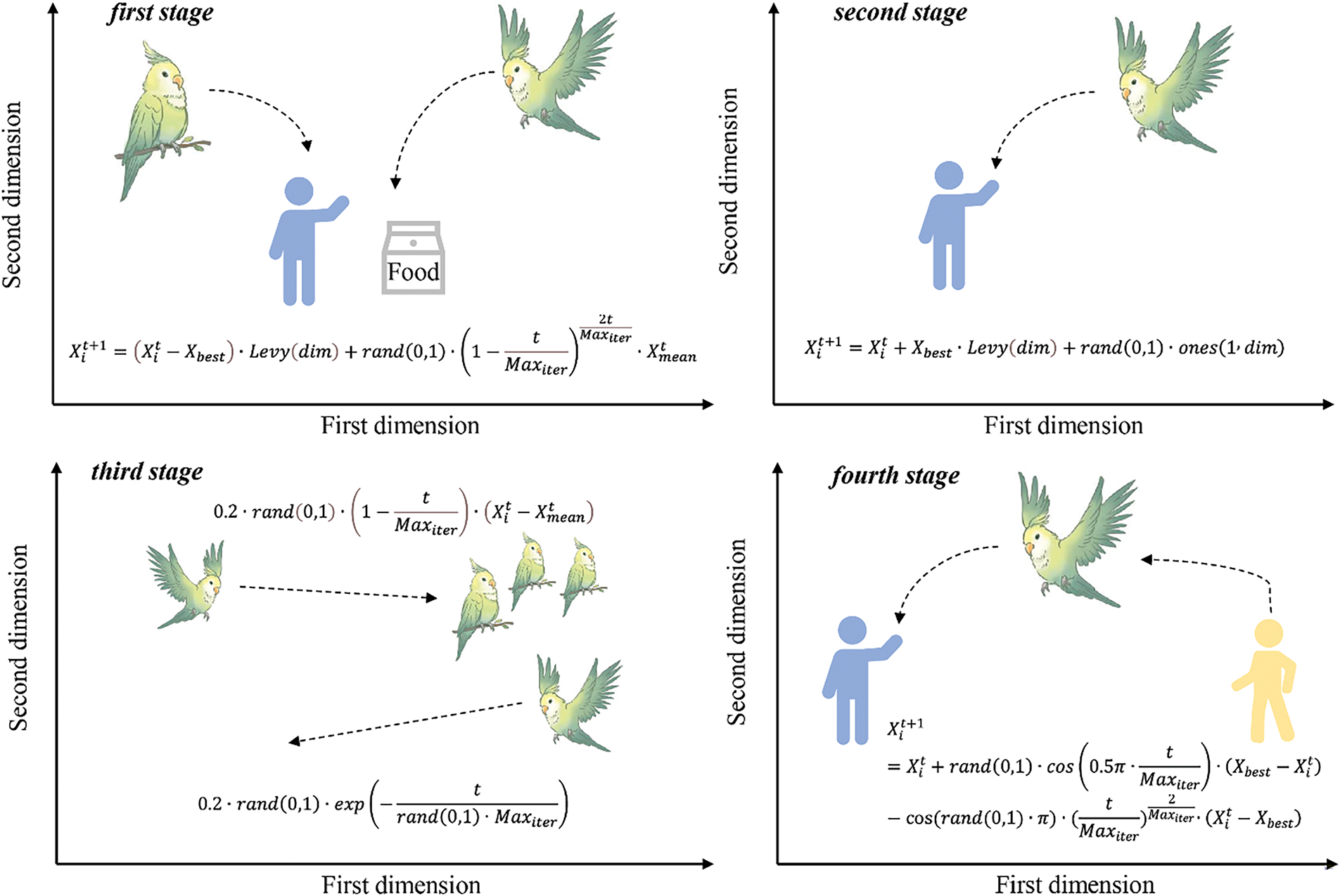
Figure 1: Schematic diagram of PO algorithm

In the first stage, the Pyrrhura Molinae performs location updates by looking at the location of the food or taking into account the location of the owner, as Eq. (3):

Xit+1=(Xit−Xbest)⋅Levy(dim)+rand(0,1)⋅(1−tMaxiter)2tMaxiter⋅Xmeant.(3)

In the second stage, Pyrrhura Molinae stays on any part of its owner’s body and remains stationary, a process that can be expressed as Eq. (4):

Xit+1=Xit+Xbest⋅Levy(dim)+rand(0,1)⋅ons(1,dim).(4)

In the third stage, Pyrrhura Molinae communicates closely within the group in two equally probable ways (flying to the flock and not flying to the flock), a process that can be expressed as Eq. (5):

Xit+1={0.2⋅rand(0,1)⋅(1−tMaxiter)⋅(Xit−Xmeant),P≤0.50.2⋅rand(0,1)⋅exp⁡(−trand(0,1)⋅Maxiter),P≥0.5.(5)

In the fourth stage, Pyrrhura Molinae parrots seek a safe location with their owners out of fear and away from strangers, with the location updated as Eq. (6):

Xit+1=Xit+rand(0,1)⋅cos⁡(0.5π⋅tMaxiter)⋅(Xbest−Xit)−cos⁡(rand(0,1)⋅π)⋅(tMaxiter)2Maxiter⋅(Xit−Xbest).(6)

2.2 Gene Expression Programming (GEP)

GEP is an efficient and advanced evolutionary algorithm designed to generate computational programs or mathematical expressions automatically [46]. The algorithm performs excellently in various data processing tasks, including regression analysis, classification, and time series prediction. In GEP, the program structure typically adopts a tree representation with two types of nodes: function nodes and terminal nodes. Function nodes perform basic operations (addition, subtraction, multiplication, and division), while terminal nodes represent input variables or constant values. The ingenuity of GEP consists of how a genetic expression encodes a program or a mathematical expression. In this process, gene expression sequences are typically strings of fixed length, each called a chromosome. GEP selects an individual’s performance using a fitness function, which measures the degree to which the program or expression solves the target problem. Genetic operations preferentially select individuals with higher fitness to form offspring so that good-quality genes can be transmitted. GEP also employs diversified strategies and methods for exploring high-quality solutions, such as genetic operations of mutation, crossover, and transposition, to improve genetic diversity in the population and avoid algorithmic premature convergence into local optimality. As iterations proceed, the gradual evolution of individuals in the population undergoes progressive development and selection of gene sequences with high expression efficiency until convergence toward the optimal solution is reached. This evolutionary process continues until a predefined termination condition is met, such as a maximum number of iterations or satisfactory fitness criteria.

The excellent performance of GEP in solving complex nonlinear problems and its unique coding mechanism provide it with clear advantages over other evolutionary algorithms in terms of flexibility and computational efficiency [47,48]. In addition, as an evolutionary algorithm capable of generating symbolic mathematical expressions, GEP is highly effective in revealing functional relationships between variables. Therefore, this study introduces GEP technology to offer transparent and interpretable structures, addressing the interpretability challenges commonly associated with ML techniques.

2.3 Model Interpretation Techniques

SHAP: SHAP (Shapley Additive exPlanations) is a powerful model interpretation technique in machine learning [49]. The SHAP calculates the contribution of each feature to model predictions by Shapley values as follows: First, it generates all possible feature subsets for every feature in the model and calculates, with and without the feature, the change in model predictions that identifies that feature’s marginal contribution. Subsequently, the overall weighted average among all subsets will ensure that the value of each feature in the model has a fair contribution. These are then combined into the SHAP values, which show precisely each feature’s contribution to the prediction’s outcome. The SHAP is mathematically represented as shown in Eq. (7) [50]:

φi=∑S⊆N∖{i}|S|!(|N|−|S|−1)!|N|!(f(S∪{i})−f(S)),(7)

where φi represents the SHAP value for feature i, S⊆N∖{i} denotes all subsets of features excluding i, |S| is the size of subset, |N| is the feature number.

PDP: The Partial Dependence Plot (PDP) model interpretation technique is used to illustrate how a specific feature (or multiple features) influences the model’s prediction output [51]. It works by averaging the possible values of all other features and plotting the impact of the chosen feature on the model’s output at different values. The core principle of PDP can be expressed by the following Eq. (8):

PDP(xj)=1N∑i=1Nf(xj,x−j(i)),(8)

where N represents the samples’ number, and f(xj,x−j(i)) is the model’s prediction function, which indicates the predicted value when the feature xj is fixed at a certain value, using the values of the other features x−j(i) from sample i.

ICE: Unlike PDP, the ICE (Individual Conditional Expectation) model interpretation technique focuses on the predicted output for each sample as the feature values change [25]. ICE is useful for displaying individual variations and is especially effective in examining how individual samples respond to changes in feature values. Additionally, ICE curves can reveal differences in the sensitivity of various samples to features and potential nonlinear or interaction effects. The following Eq. (9) can be used to express this:

ICEi(xi)=f(xj,x−j(i)),(9)

where f(xj,x−j(i)) represents the model prediction when the feature xi is fixed at a certain value, while the values of the other features x−j(i) in sample i remain unchanged.

2.4 Model Evaluation Metrics

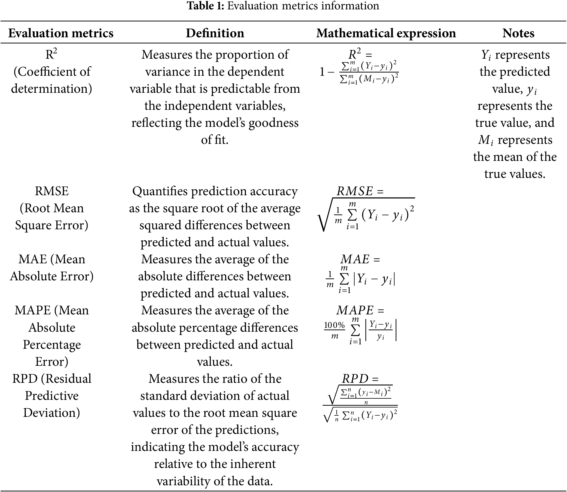
Evaluating model performance is crucial for validating its effectiveness in real-world applications. This process examines the model’s accuracy, stability, and consistency, uncovers potential areas for improvement, and identifies underlying issues. A thorough analysis of the evaluation results can highlight the model’s strengths and weaknesses, providing valuable insights for subsequent optimization efforts, thereby ensuring its adaptability and reliability in practical environments. In this study, we aim to provide a comprehensive evaluation of the model’s predictive performance, with a particular focus on its goodness of fit, prediction errors, accuracy, and stability. Therefore, five evaluation metrics were employed to assess the proposed model: R2 (Coefficient of Determination), RMSE (Root Mean Square Error), MAE (Mean Absolute Error), MAPE (Mean Absolute Percentage Error), and RPD (Residual Predictive Deviation), as outlined in Table 1. These metrics, as established and widely used in statistical analysis, are representative and have been applied across various domains to evaluate model performance [52–54].

3  Data Acquisition and Verification

3.1 CO2-UCS Database

To ensure the robustness and generalization of models, a comprehensive and scientifically sound database is needed. Therefore, for predicting CO2-induced strength, this study extensively collected UCS test results from previous studies and established the CO2-UCS database. A crucial step in this process was determining the model’s input parameters. According to the studies, CO2 saturation pressure (P) significantly affects coal seams’ UCS and elastic modulus [17,55,56]. As a result, we have selected CO2 saturation pressure, P, as one of the input parameters. The interaction time, T, between CO2 and coal seams was also shown to be essential in altering UCS [57]. Since all the tests mentioned in the literature were conducted on different coal types, the coal type should be an input parameter. Further, it was shown that even while the same CO2 saturation pressure and interaction time are applied, a significant difference in strength changes may exist for different coal samples [19]. In such a way, coal type was considered one of the key factors that affect the CO2-induced strength. Typically, coal classification is based on its degree of coalification, which refers to the maturation level of coal [58]. As the degree of coalification increases, the carbon content in coal rises, while the volatile matter decreases. This results in higher calorific value and improved combustion performance. The carbon content directly affects the coal’s calorific value and energy release efficiency, making it an important indicator for coal classification. Therefore, different coal types were characterized using fixed carbon content (FC), a widely recognized method in the field of coal research [22].

Furthermore, research has shown that the unique properties of CO2 (such as adsorption capacity, diffusivity, viscosity, and phase transitions) can alter the micro-structure of coal seams, leading to changes in strength [59–62]. However, incorporating these properties as input parameters is not optimal. Measuring CO2 properties typically requires time-consuming and labor-intensive experimental methods, such as gas adsorption experiments, self-diffusion experiments, etc. [63]. This makes such data difficult to obtain and has led to limited research in this area, preventing the establishment of a large-scale database. Moreover, these parameters are not essential; the two input parameters (P and T) are sufficient to assess the impact of CO2 on coal strength. Therefore, this study determines three key input parameters: CO2 interaction time (T), CO2 saturation pressure (P), and fixed carbon content (FC), with UCS as the target for prediction. It is noteworthy that, in all experiments, the parameters T and P were independent of each other, meaning the value of P remained constant and was not influenced by variations in T.

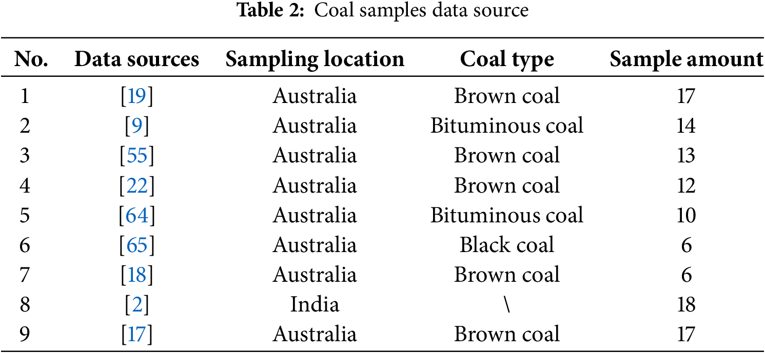
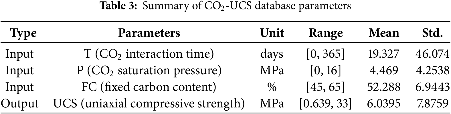
The CO2-UCS database is now complete, containing a total of 113 data entries. Data source information is provided in Table 2, and statistical details are presented in Table 3. As shown in Table 3, the parameters in the CO2-UCS database exhibit the following value ranges: T spans from 0 to 365 days, P ranges from 0 to 16 MPa, and FC varies between 45% and 65%. Although the dataset is relatively small in size, it nearly encompasses all plausible combinations of these parameters under practical conditions. Thus, the database can be considered sufficiently comprehensive for the purpose of this study, providing a robust foundation for model development and validation.

3.2 Data Verification

Before establishing the model, it is crucial to validate the database thoroughly. We employed a correlation scatter matrix to identify any outliers in the target variable UCS and to examine the relationships between the input parameters and the target variable, ensuring the data’s validity and reliability. According to the data distribution (lower triangular matrix) in Fig. 2, no significant outliers were detected in UCS, indicating high data quality. In addition, in the correlation matrix, the values in the far-right column represent the correlations between the prediction target, UCS, and the input parameters P, FC, and T, with values of −0.16, 0.87, and −0.19, respectively. This suggests that parameter FC has a strong positive correlation with UCS, while parameters P and T show weak negative correlations. These correlations provide initial support for the selection of these input parameters. Regarding the correlation between input parameters, it helps assess potential redundancy. In this database, the highest correlation between input parameters is observed between parameters P and T (0.29), which is a weak correlation, indicating that no significant redundancy exists among the input parameters. Overall, the data in the CO2-UCS database demonstrates good performance in terms of correlation and the absence of outliers. Therefore, the CO2-UCS database established in this study is considered reliable and can be used for subsequent model training and predictive analysis.

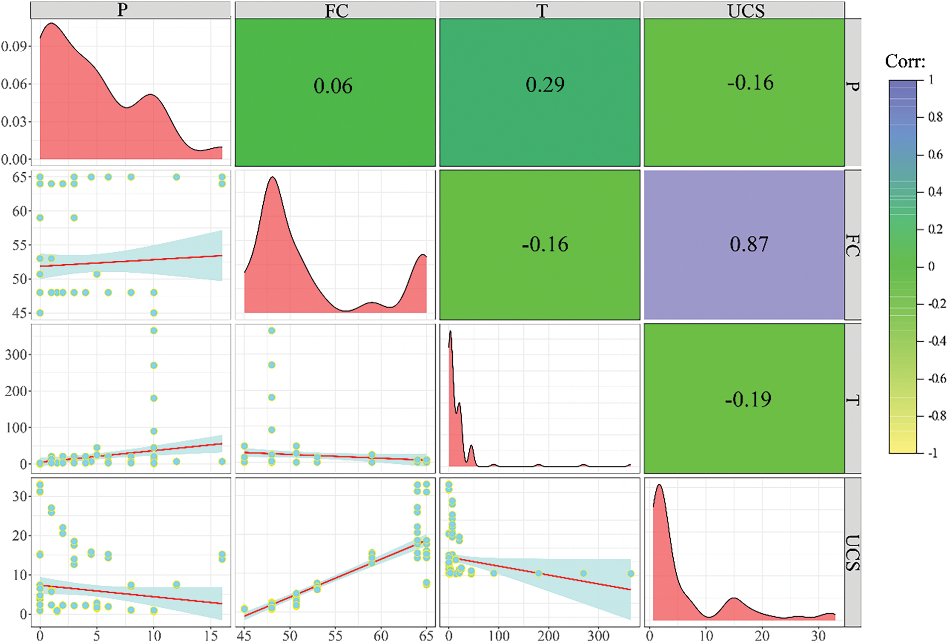
Figure 2: Distribution and correlation of parameters

4  Model Construction

The construction of the CO2-induced strength prediction models consists of four stages: data processing, setting intelligent algorithm model parameters, developing intelligent algorithm prediction models, and establishing the GEP prediction models, as shown in Fig. 3.

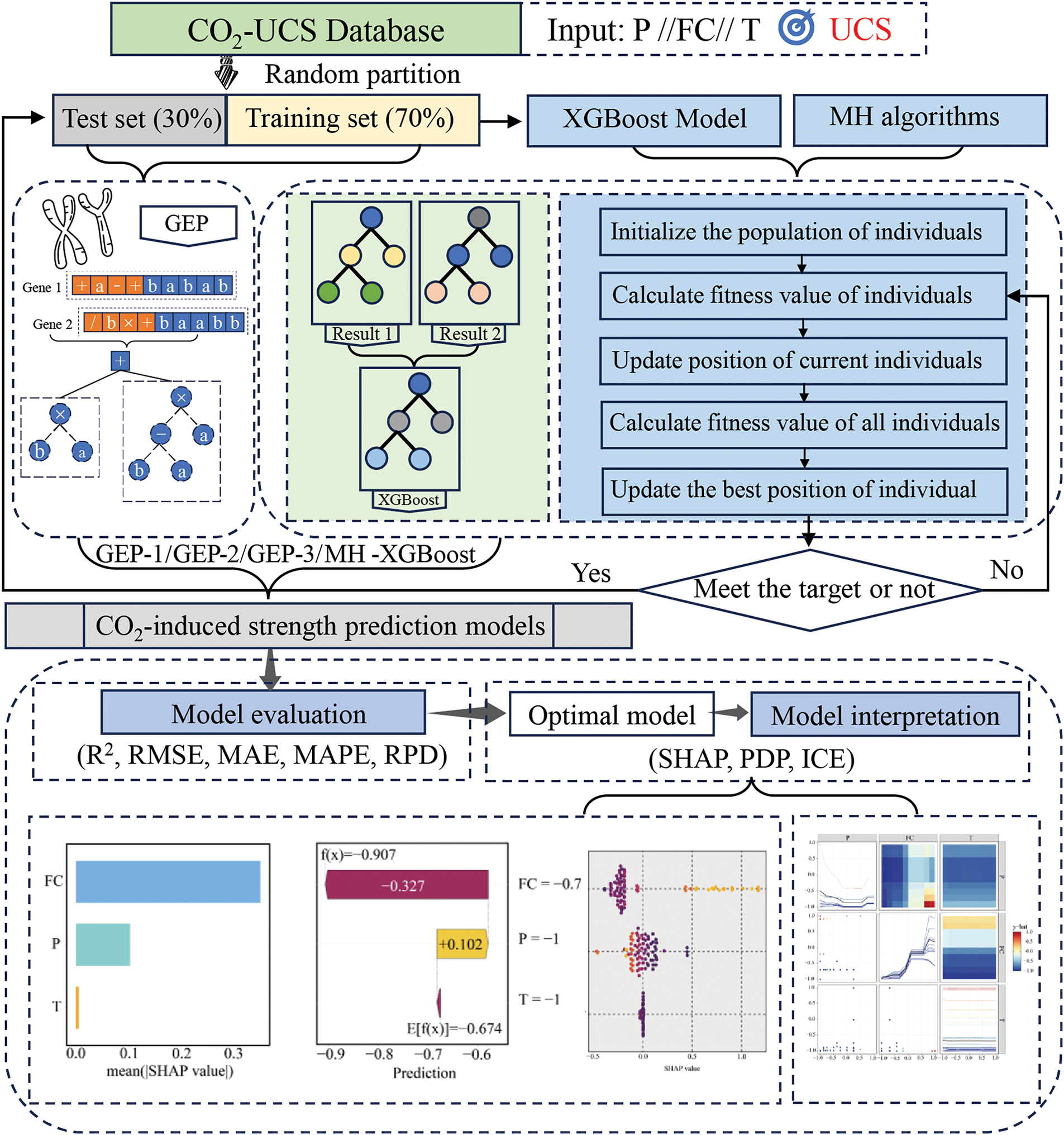
Figure 3: CO2-induced strength prediction models’ construction

First stage: data processing.

The dataset was randomly divided into training and test sets in a 7:3 ratio for model training and evaluation. During this process, it is critical to ensure that both subsets maintain a consistent distribution. This consistency enhances the model’s generalization capability, enabling it to robustly handle noise and bias in the data [66].

Fig. 4a–d displays the distributions of parameters P, FC, T, and UCS across training set (80) and test set (33). For parameter P, the mean values are 4.03 and 5.55 for the training and test sets, respectively, with a slight increase in the testing set but overall similar distributions. Parameter FC shows mean values of 51.95 for the training set and 53.11 for the test set, indicating consistent distributions. For parameter T, the means are 18.23 in the training set and 22.00 in the test set, with both distributions remaining reasonable despite the higher mean in the test set. Lastly, UCS has mean values of 5.88 for the training set and 6.42 for the test set; while the testing set includes fewer high values, its distribution aligns well with the training sets. Overall, all features exhibit consistent distributions between the training and test sets, demonstrating the high quality of the data split and its suitability for subsequent model training. Additionally, a standard data preprocessing technique was employed, where all data were normalized to the range of [−1, 1] during the model training phase. It is worth noting that the normalization process was performed separately, meaning that normalization was applied only to the training set. For the test set, normalization was conducted using the maximum and minimum values derived from the training set. This approach prevents potential data leakage, ensuring that the test set can effectively serve as a validation set, which contributes to improving the model’s generalization capability.

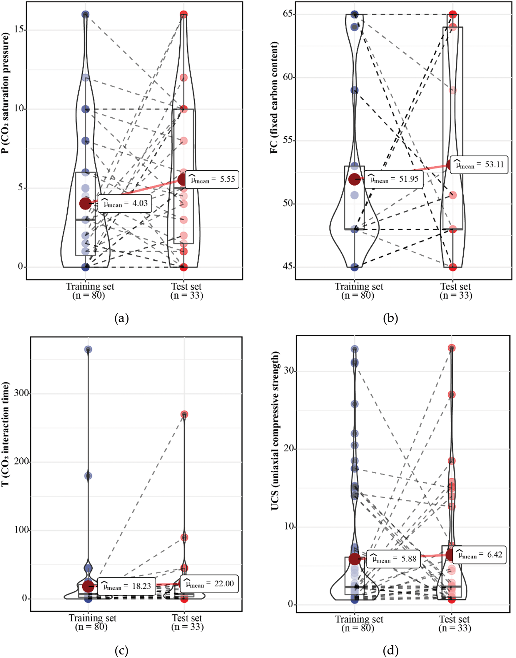
Figure 4: Training and test sets distribution of CO2-UCS dataset: (a) P; (b) FC; (c) T; (d) UCS

Second stage: setting intelligent algorithm model parameters.

This study explored the use of three MH algorithms to optimize the hyperparameter space of the XGBoost model. The hyperparameters optimized in the XGBoost model include num-trees (number of iterations), max-depth (tree depth), and eta (learning rate). First, the hyperparameter ranges were defined as [1, 100] for num-trees, [1, 5] for max-depth, and [0.01, 0.5] for eta to avoid unnecessary computational resource consumption. Second, the population size for the population-based MH algorithms was determined. This study evaluated four population sizes (25, 50, 75, and 100) to ensure the algorithm possesses strong global search capabilities while mitigating the risk of local optima. During the entire process, the number of model iterations was fixed at 200.

Third stage: development of the MH-XGBoost prediction models.

The present work used three MH optimization algorithms to find the best hyperparameter combination: GWO, SSA, and PO. This is initiated by training the model using the training set. Optimization began by initializing the individual population, where candidate combinations of hyperparameters are generated randomly. Then, the fitness value for each of these needs to be calculated to evaluate the model’s performance. According to the search mechanism of the MH algorithms, each individual position was updated dynamically to explore the space to search, and the optimal position and global solution were then iteratively refined. This iterative process continued until the termination condition, defined as the maximum number of iterations, was reached. Finally, the performance of the established MH-XGBoost model (GWO-XGBoost, SSA-XGBoost, and PO-XGBoost) was evaluated by using the test set.

Fourth stage: development of the GEP prediction models.

In this study, Gene Expression Programming (GEP) prediction models were developed to complement and benchmark the proposed MH-XGBoost prediction models. The GEP models were constructed using the same CO2-UCS database, following a systematic process: First, an initial population of randomly generated chromosomes was created. These chromosomes were evolved through genetic operations, including selection, crossover, mutation, and transposition. Subsequently, the performance of each chromosome was assessed using a fitness function. The iterative optimization process continued until the maximum number of iterations was achieved, after which the chromosome with the highest fitness was selected as the final prediction model. Finally, a total of three GEP models were established in this paper.

5  Results and Analysis

5.1 MH-XGBoost Models’ Performance

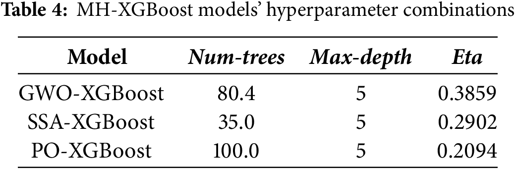
In the MH-XGBoost models, four population sizes (25, 50, 75, and 100) in MH algorithms were tested. However, experimental results indicated that a population size of 25 was sufficient to achieve excellent performance. In this study, increasing the population size only significantly prolonged the computation time without notably improving model performance. Therefore, the population size for all three MH algorithms (GWO, SSA, and PO) was set to 25. Fig. 5 illustrates the fitness curves of the GWO-XGBoost, SSA-XGBoost, and PO-XGBoost models. As depicted, all models converged to their lowest fitness values within the first 50 iterations, demonstrating that the hyperparameter configurations quickly approached their optimal settings. The specific hyperparameter combinations for each MH-XGBoost model are comprehensively detailed in Table 4.

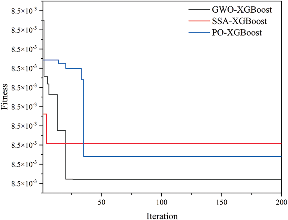
Figure 5: Fitness of MH-XGBoost prediction models

With the optimal hyperparameter configurations, an initial evaluation of the model’s performance was conducted to validate its predictive accuracy for CO2-induced strength. The scatter plot regression analysis in Fig. 6 visually compares the actual and predicted values for the training and test sets. In the figure, each model point’s position is determined by the predicted values on the y-axis and the measured values on the x-axis. The red region represents the fitted range of all model points, while the black dashed line denotes the ideal fit (i.e., the 1:1 line between actual and predicted values). Additionally, the marginal histograms illustrate the distribution of data points, providing insights into the concentration trends and deviations across different value ranges.

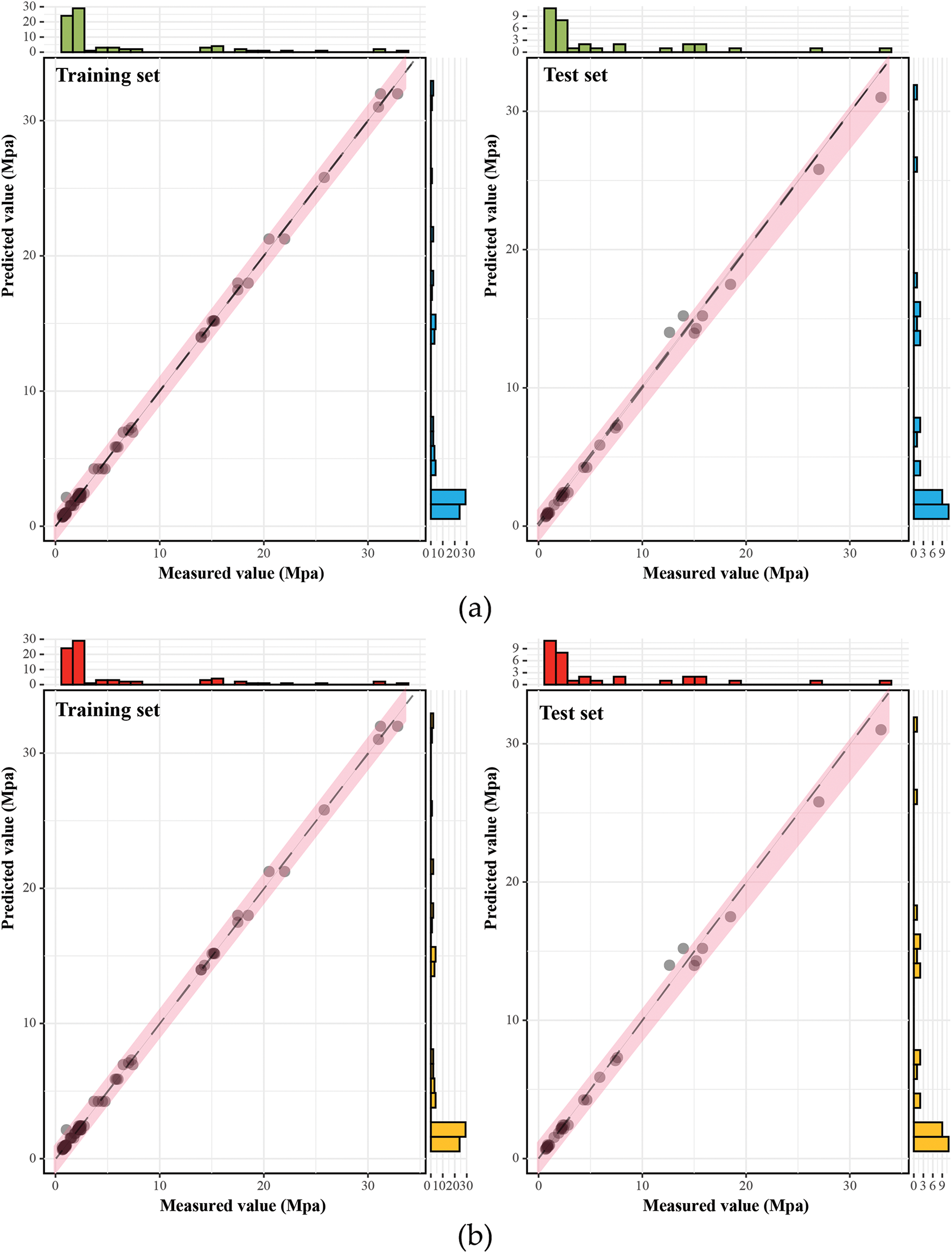
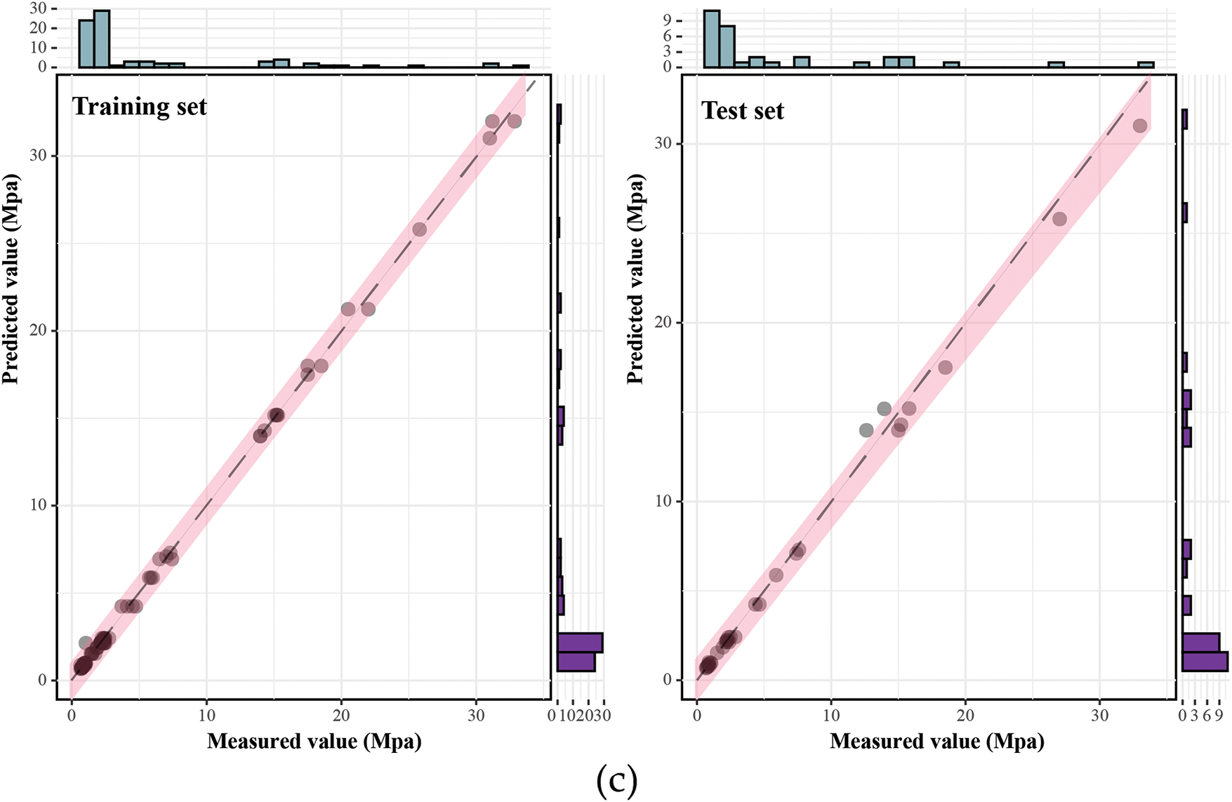
Figure 6: Performance evaluation of MH-XGBoost models: (a) GWO-XGBoost model; (b) SSA-XGBoost model; (c) PO-XGBoost model

Fig. 6a illustrates the GWO-XGBoost model’s predictive accuracy on training and test datasets, with scatter points primarily within the red fit region and closely aligned with the black dashed 1:1 ideal fit line. The training data set has a minor prediction error and a narrow range of fits, while the test data set retains a strong generalization ability despite slightly higher errors. In addition, the edge histogram confirmed a high degree of agreement between the predicted and actual values, confirming the reliability of the model for the prediction of CO2-induced strength. Furthermore, Fig. 6b depicts the performance of the SSA-XGBoost model, where the scatter points are tightly clustered near the 1:1 ideal fit line between the two data sets, indicating high prediction accuracy. The error recorded in the test set was slightly higher than in the training dataset, but the model showed strong generalization ability. The marginal histograms underscore the model’s aptitude in capturing the distributions effectively, particularly in lower value ranges. Fig. 6c reveals that the PO-XGBoost model achieves outstanding predictive accuracy, with a performance alignment suggesting a high degree of model effectiveness across different datasets.

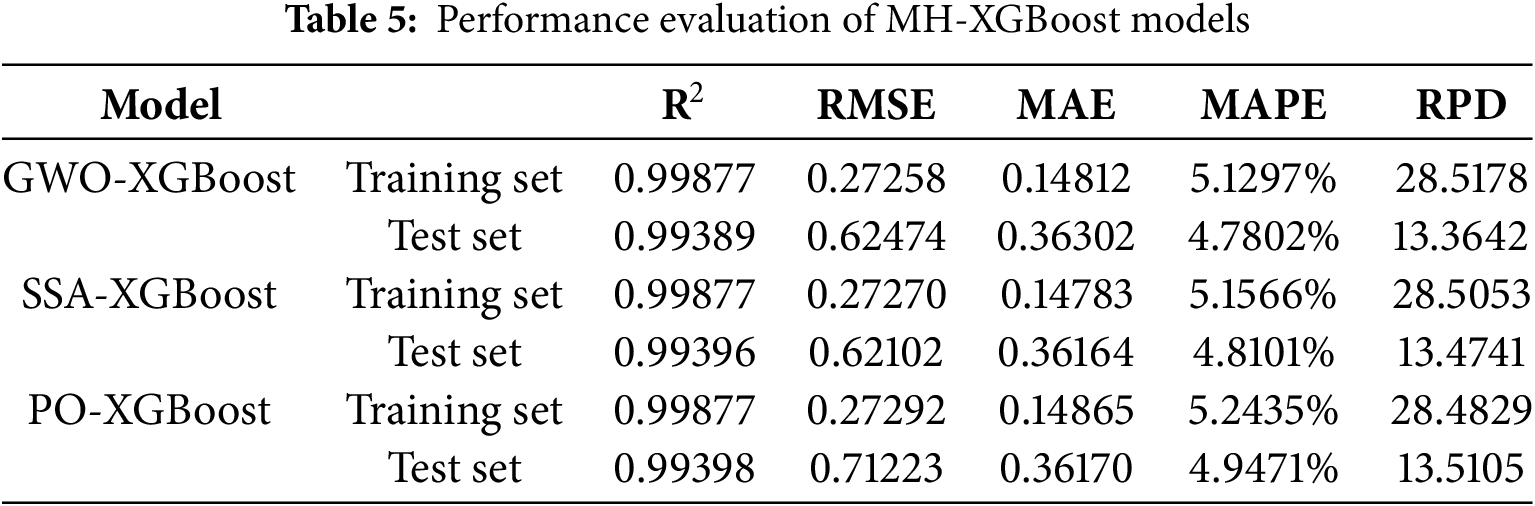
The predictive performance of these models was further evaluated using five metrics, as shown in Table 5. All models demonstrated very high goodness of fit on the training and test sets, with R2 values approaching 1, indicating that the models effectively captured the data’s variance. In terms of RMSE, the SSA-XGBoost model performed best on the test set (RMSE = 0.62102), slightly outperforming the GWO-XGBoost model (RMSE = 0.62474). The PO-XGBoost model exhibited a higher RMSE, suggesting a slightly weaker performance on the test set. For MAE, SSA-XGBoost achieved the lowest values on both the training set (MAE = 0.14783) and the test set (MAE = 0.36164), indicating minimal absolute error. Regarding MAPE, the GWO-XGBoost model performed slightly better on both datasets, with the lowest test set MAPE (4.7802%), demonstrating the minor relative prediction error. For RPD, all models achieved values significantly greater than 10, reflecting strong predictive capabilities. Among them, GWO-XGBoost exhibited an RPD of 13.3642 on the test set, slightly lower than that of SSA and PO. In conclusion, all three MH-XGBoost models demonstrated remarkable performance across all evaluation metrics.

5.2 GEP Models’ Performance

In constructing the GEP prediction models, the same training set was used to generate the CO2-induced strength prediction formula, while the test set was employed to evaluate the robustness of the formula. A total of three GEP models were developed, as shown in Table 6. Fig. 7a illustrates the fitness curves of the three GEP models over 1500 iterations. These curves reveal that after approximately 300 iterations, the fitness values stabilized and remained constant, indicating that the models had converged at this stage. Further iterations did not significantly enhance the models’ performance, suggesting that the optimization process had reached its optimal solution. The corresponding gene expression trees, which provide an intuitive visualization of the models’ predictive mechanisms, are presented in Fig. 7b–d.

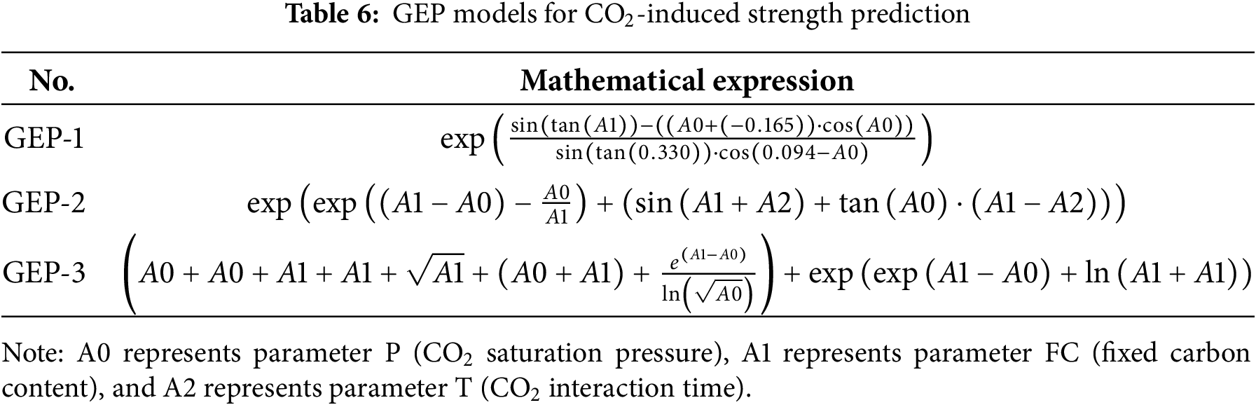
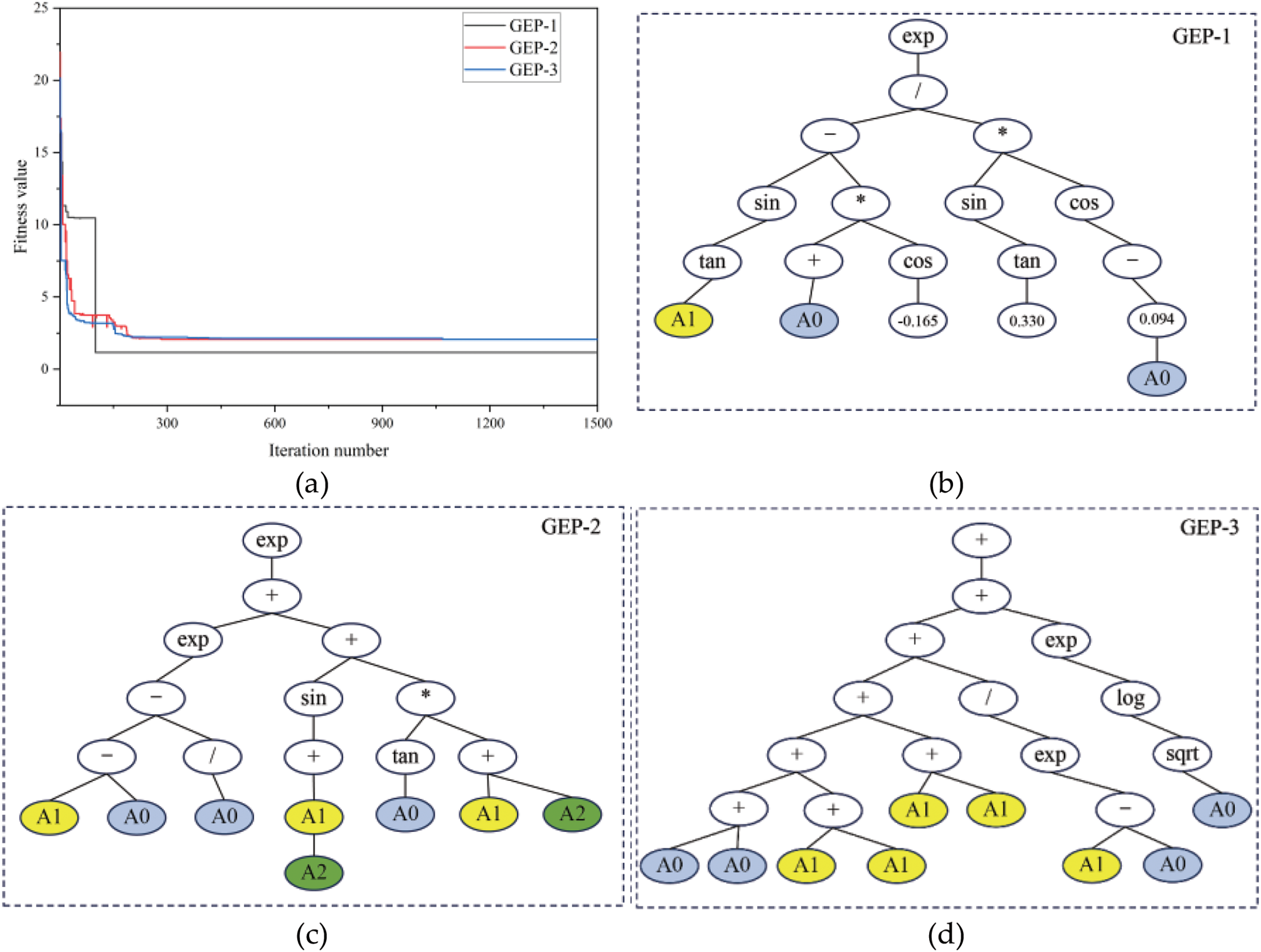
Figure 7: Fitness curves and corresponding gene expression trees for the GEP models: (a) fitness curves; (b) GEP-1 model; (c) GEP-2 model; (d) GEP-3 model

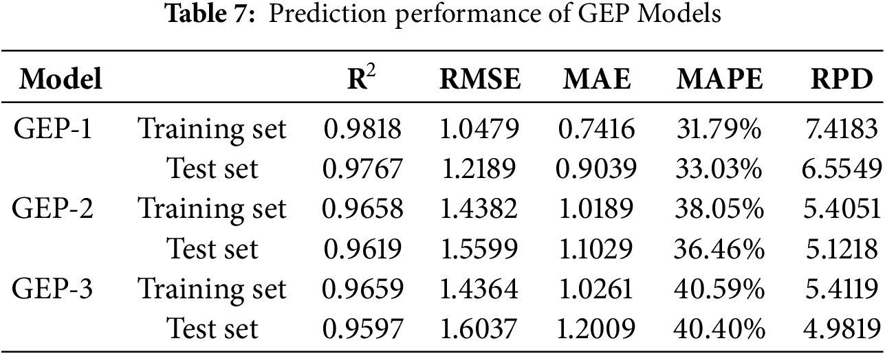
The scatter plot regression analysis in Fig. 8 preliminarily demonstrates that all three GEP models exhibit high goodness of fit on the training and test sets. A further evaluation of the model’s performance using five metrics is summarized in Table 7. Among them, the GEP-1 model achieved the best performance on both the training and test sets, with R2, RMSE, MAE, MAPE, and RPD values of (0.9818, 0.9767), (1.0479, 1.2189), (0.7416, 0.9039), (31.79%, 33.03%), and (7.4183, 6.5549), respectively.

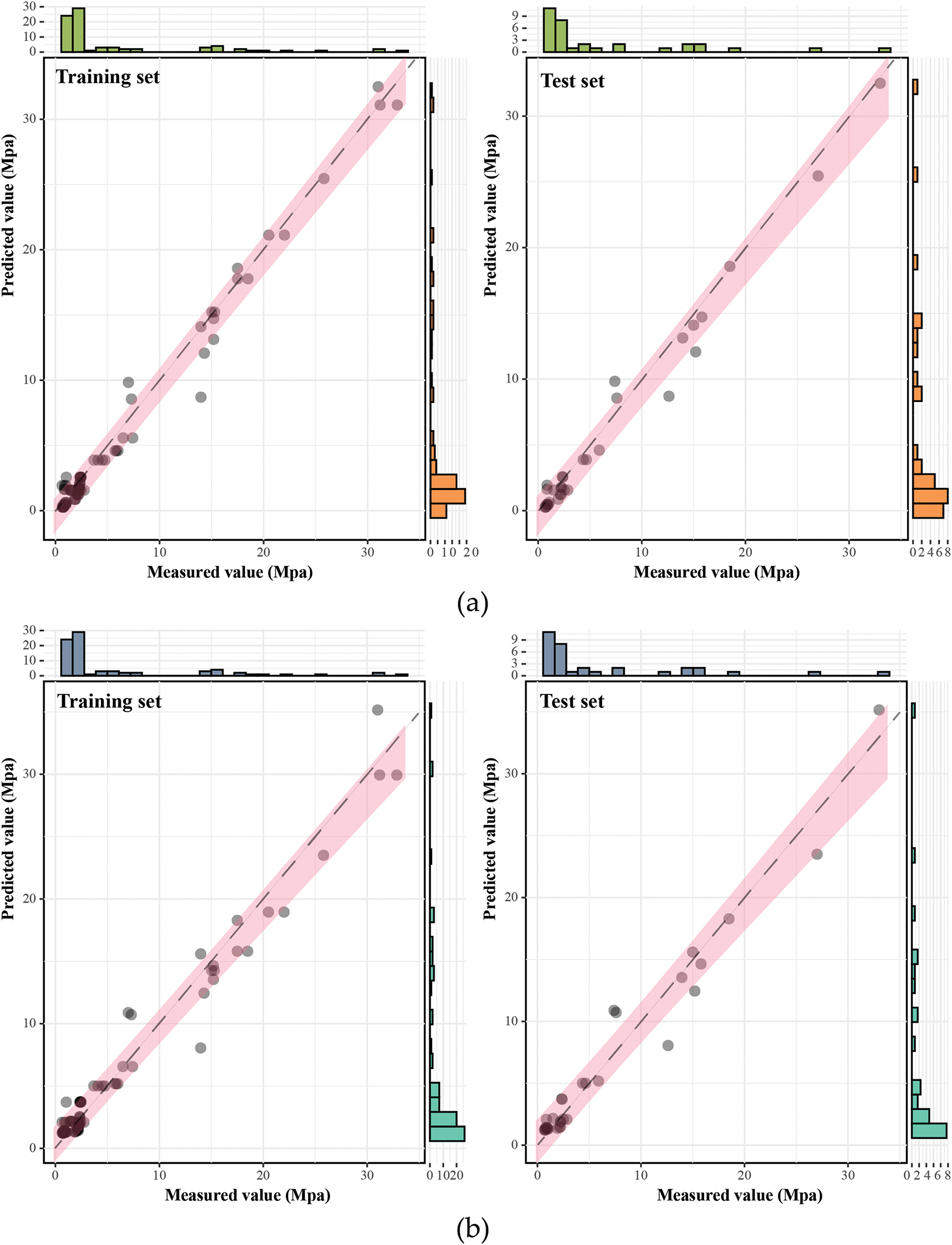
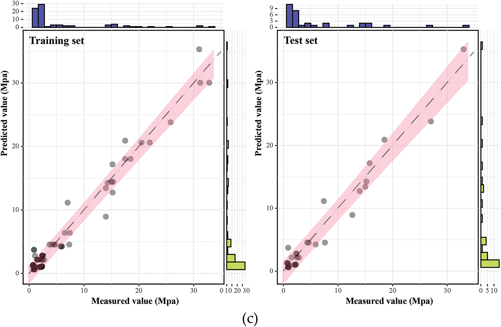
Figure 8: Performance evaluation of GEP models: (a) GEP-1 model; (b) GEP-2 model; (c) GEP-3 model

5.3 Model Performance Comparison

As outlined earlier, this study first developed three XGBoost-based predictive models (GWO-XGBoost, SSA-XGBoost, and PO-XGBoost) and subsequently constructed three GEP predictive models (GEP-1, GEP-2, and GEP-3). All six models demonstrated excellent predictive performance: on the training set, R2 > 0.96, RMSE < 1.44, MAE < 1.03, MAPE < 40.60%, and RPD > 5.12; on the test set, R2 > 0.95, RMSE < 1.61, MAE < 1.21, MAPE < 40.40%, and RPD > 4.98. Despite these impressive results, a comprehensive comparison is necessary to identify the best predictive model. This step is crucial not only for enhancing predictive accuracy but also for improving interpretability and supporting decision-making in practical applications, particularly in optimizing model structures and parameter selection.

Firstly, the error analysis of all models on the test set is carried out. As shown in Fig. 9, the line chart shows the true value of the predicted target (UCS) compared to the predicted value, and the bar chart represents the size of the error. In MH-XGBoost models, not only the true value and the predicted value have a very high degree of fit, but also the maximum error is only about 2.0. In contrast, the GEP model has a maximum error of about 4.5. Error analysis results show that MH-XGBoost models have higher prediction accuracy and smaller prediction error than GEP models, which are the superior models.

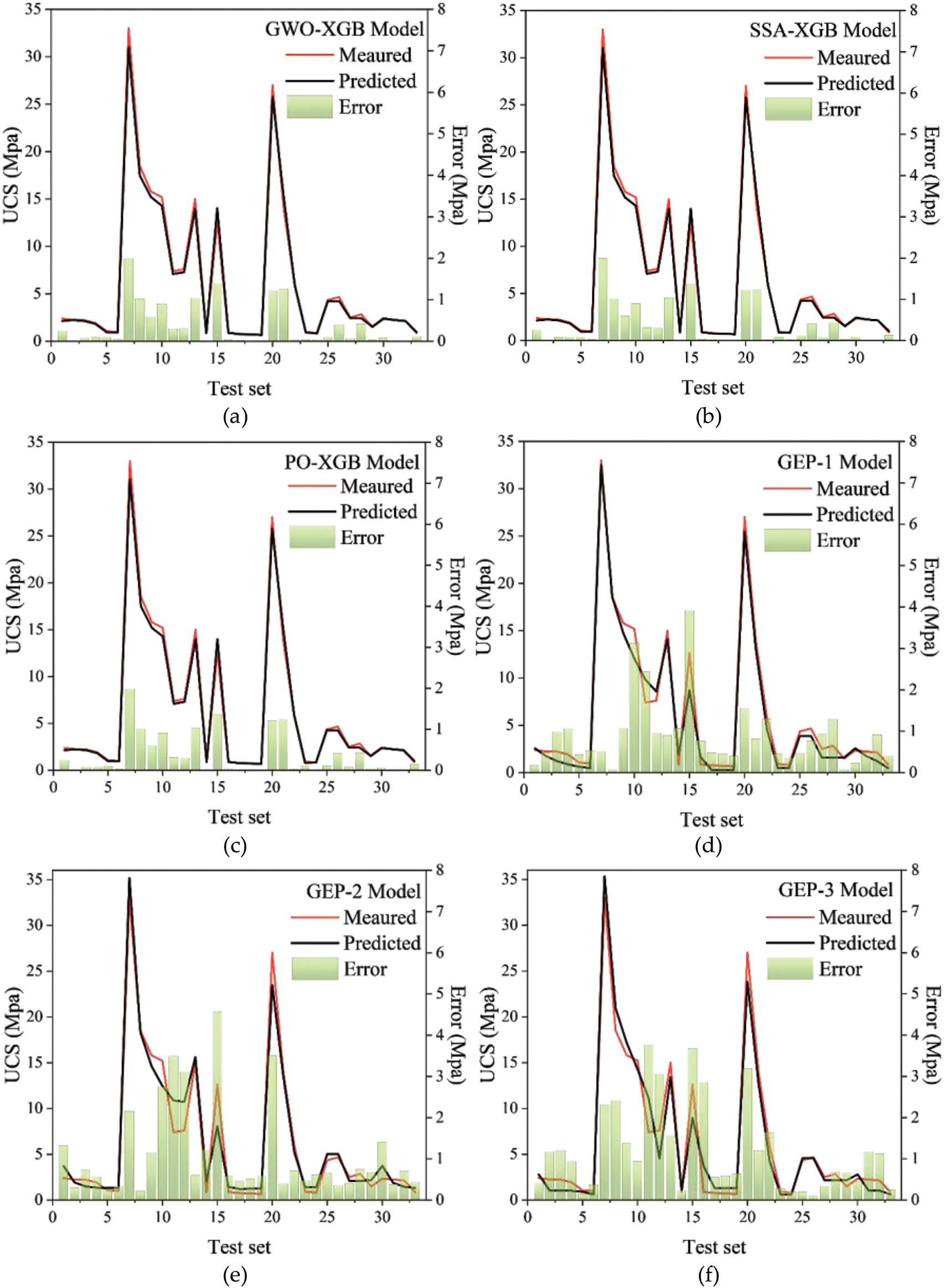
Figure 9: Error analysis on test set: (a) GWO-XGBoost model; (b) SSA-XGBoost model; (c) PO-XGBoost model; (d) GEP-1 model; (e) GEP-2 model; (f) GEP-3 model

Secondly, this study first employed non-parametric statistical testing to compare the statistical differences among models. Additionally, a dynamic global performance indicator was introduced to comprehensively assess the performance of each model, ultimately identifying the optimal predictive model.

In this study, the Friedman test for multiple comparisons has been used to test the differences among the models. The obtained Critical Difference (CD) value is utilized to decide whether the differences among the groups are statistically significant [67–70]. That is, if the difference between the two models is higher than the value of CD, the performance will be significantly different. In this study, with a significance level of 0.05, the number of models k = 6, and the number of evaluation metrics N = 5, the calculated CD value was 2.65. Thus, for the two models, if the rank difference is greater than 2.65, it is said that their performance differs significantly. As indicated in Fig. 10, both GWO-XGBoost and SSA-XGBoost outperform the GEP-2 and GEP-3 models significantly, while the PO-XGBoost performs significantly better than the GEP-3 model. There is no significant difference between the GWO-XGBoost, SSA-XGBoost, PO-XGBoost, and GEP-1 models, which shows that these models can be considered preliminary optimal models.

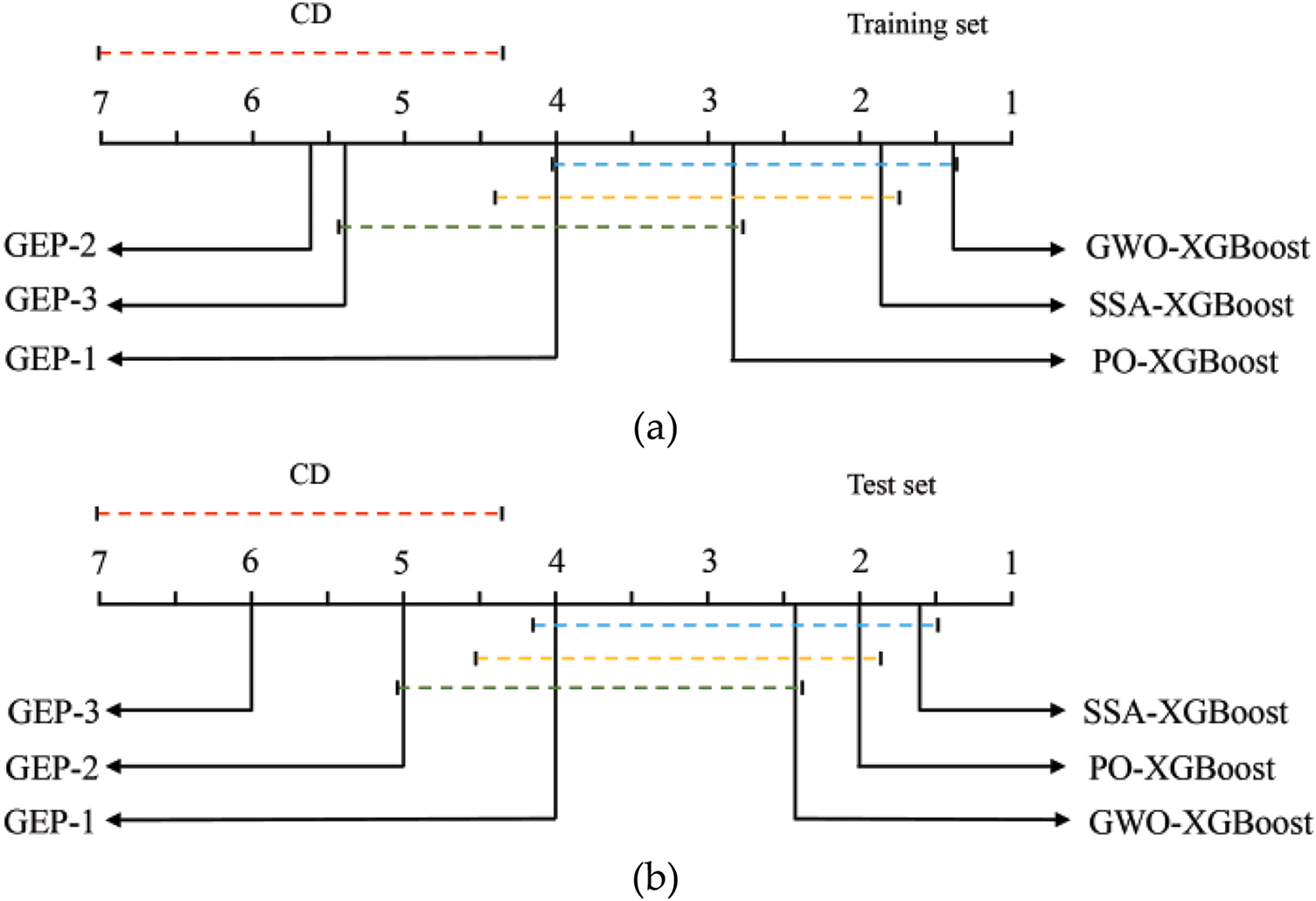
Figure 10: Critical Difference comparison of proposed CO2-induced strength prediction models: (a) training set; (b) test set

To further assess the performance differences among the models, an improved dynamic global performance indicator (D-GPI) was introduced for detailed comparison. The D-GPI enhances the traditional GPI by dynamically assigning weights based on variance, ensuring a more comprehensive and accurate evaluation. The improved formula is presented in Eq. (10):

D−GPIi=∑j=16(φj⋅ωj(med(NorIndexj)−NorIndexij)),(10)

where φj is the sign for the j-th metric, equal to 1 for metrics like MAE, MAPE, and RMSE, and −1 for metrics like R² and RPD. ωj is the weight for the j-th metric, dynamically assigned based on the variance of that metric, with the weight proportional to the variance. NorIndexj is the normalized value of the j-th metric. NorIndexij is the normalized value of the j-th metric for model i. med(NorIndexj) is the median of the normalized values of the j-th metric.

Weights corresponding to each evaluation criterion in D-GPI are adjusted dynamically by variances to ensure the generality of the overall assessment. The system gives higher weight to criteria whose variance is higher (which means high variability), giving full significance to such metrics in determining the overall score. This weighting mechanism allows D-GPI to mirror the relative importance between different metrics better. A higher overall score indicates better model performance. As shown in Fig. 11, the ranking of the models based on D-GPI is as follows: SSA-XGBoost (0.3501) > GWO-XGBoost (0.3460) > PO-XGBoost (0.3328) > GEP-1 (−0.3282) > GEP-2 (−0.5792) > GEP-3 (−0.6487).

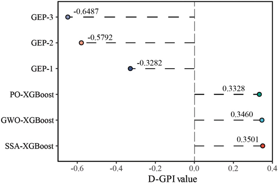
Figure 11: Comparative evaluation of models based on D-GPI

5.4 Model Application Development

This study successfully developed the MH-XGBoost and GEP models, which enable precise and efficient predictions of CO₂-induced alterations in coal strength. However, code-based models are often tedious and complex for practitioners to implement in engineering applications. To enhance the practical applicability of the models, a MATLAB-based application (APP) was developed. This application seamlessly integrates input data and provides real-time predictions of changes in coal strength. As shown in Fig. 12, the application features a user-friendly interface and interactive functions, allowing users to visualize and adjust parameters and simulate various operational scenarios. The tool aims to support decision-making in research and industrial applications, facilitating the safe and efficient management of activities such as CO₂ sequestration and coalbed methane extraction.

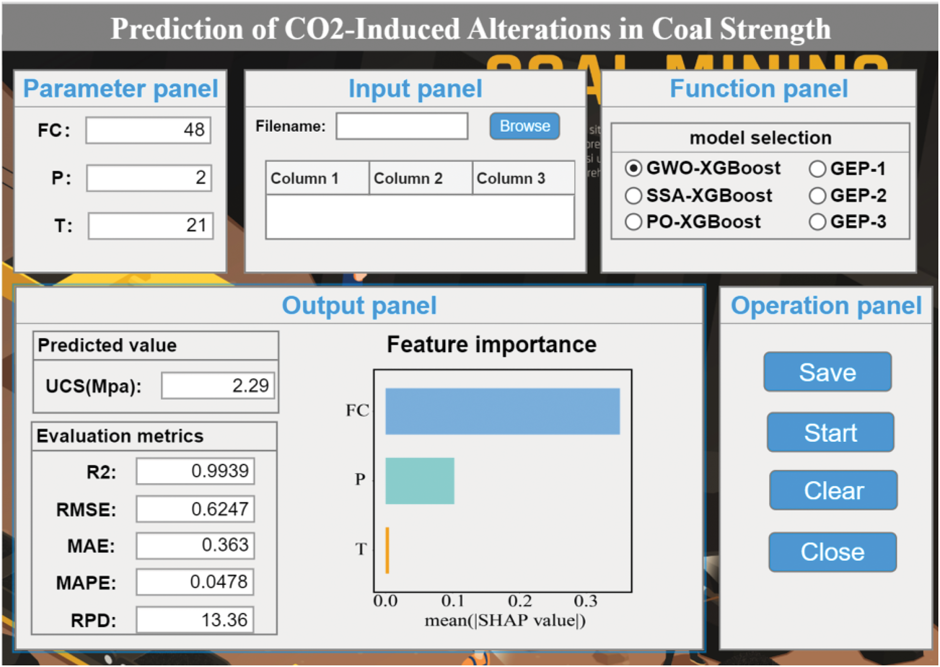
Figure 12: MATLAB-based application (APP) for predictions of CO₂-induced alterations in coal strength

6  Model Interpretation Analysis

Due to the impossibility of directly understanding either the decision-making process or the degree to which the different features of the input have contributed to the predictions, ML models are often referred to as “black boxes” [71]. Hence, their post-hoc explanations using model interpreters become critically important. Such explanations make the model more transparent and provide useful information for optimization and debugging. By interpreting the internal mechanism, we can know the feature relationships to ensure the model is reliable and fair for complex decision-making scenarios [72]. As previously discussed, the interpretation techniques (SHAP, ICE, and PDP) were introduced to explain the optimal CO2-induced strength prediction model developed in this study: the SSA-XGBoost model.

Fig. 13a illustrates the overall importance of parameters based on the mean absolute SHAP values. Among these, the parameter FC has the highest mean SHAP value, indicating its dominant influence on model predictions, followed by P and T. In addition, Fig. 13b presents a waterfall chart that decomposes a specific instance’s prediction into contributions from individual SHAP values. In the chart, the horizontal axis represents the cumulative effect of SHAP values, with f(x) denoting the prediction (−0.907) and E[f(x)] representing the model’s baseline value (−0.674). Starting from the baseline, FC contributes −0.327, lowering the prediction, while P contributes +0.102, slightly increasing the value. This visualization highlights the role of specific features in driving the prediction outcome for an individual instance. Moreover, Fig. 13c depicts the relationship between SHAP values and parameter values for each sample. Each point represents a sample, with color indicating the parameter value (yellow for higher values and darker shades for lower values). SHAP values indicate the magnitude and direction of a feature’s contribution to the model prediction. Positive SHAP values signify a positive contribution to the model output, while negative values indicate a negative contribution. The detailed analysis is as follows:

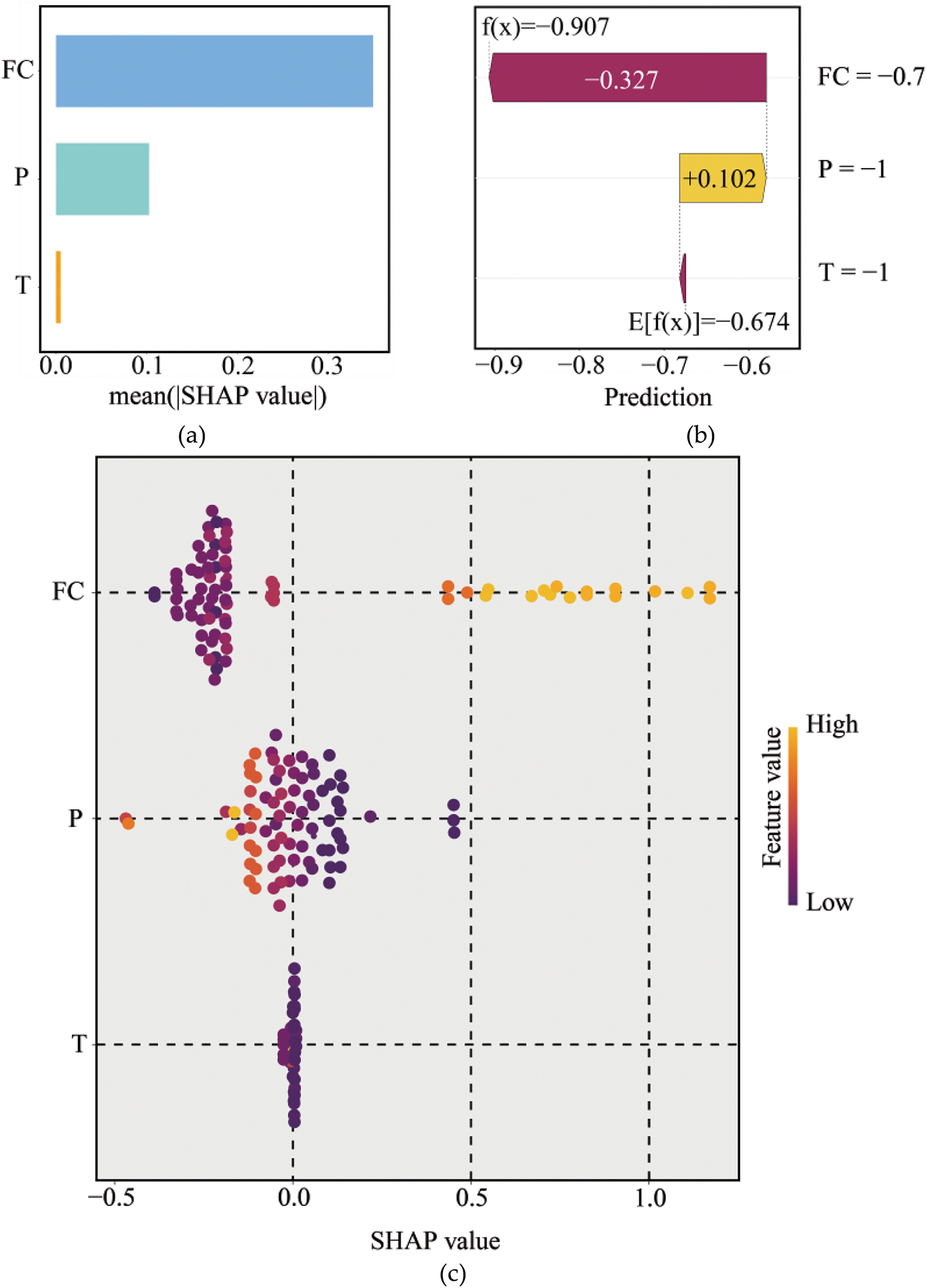
Figure 13: SHAP-based interpretation of the SSA-XGBoost model: (a) importance of parameters; (b) specific instance’s prediction; (c) relationship between SHAP values and parameter values

FC: When the FC value is low, the SHAP value is negative, indicating a negative contribution to the prediction results. As the FC value increases, the SHAP value also increases and becomes positive, suggesting a positive contribution to the prediction results.

P: In contrast to FC, high values of P (indicated by yellow) generally exhibit a negative contribution to the prediction results, while low values (indicated by dark purple) often show a positive contribution.

T: The SHAP values for T are generally small and concentrated near zero, suggesting its relatively minor impact on the model output.

In conclusion, FC emerges as the most impactful parameter with a clear positive correlation to the predictions, while P plays a secondary but significant role with an inverse effect. T has a negligible influence on the predictions.

Fig. 14 presents the feature dependence plots generated using the SHAP interpreter. Fig. 14a illustrates the relationship between parameter FC and its SHAP values, with the color representing the values of parameter P. The plot shows an increasing trend in SHAP values as FC increases, indicating that higher FC values contribute more positively to the model output. In contrast, lower FC values are associated with SHAP values that are either negative or close to zero, suggesting that FC has little to no positive impact on the model output when its value is low. This observation aligns with the previous analysis. Next, the interaction effects between FC and P are examined. The color gradient, ranging from purple to yellow, represents the values of P, from low to high. When FC values are high, the color of the points shifts from yellow to purple, indicating that lower P values amplify the positive influence of FC on SHAP values, resulting in a stronger positive contribution to the model output. Conversely, when FC values are low, decreasing P values correspond to lower SHAP values, which are predominantly negative, indicating a negative contribution to the model output.

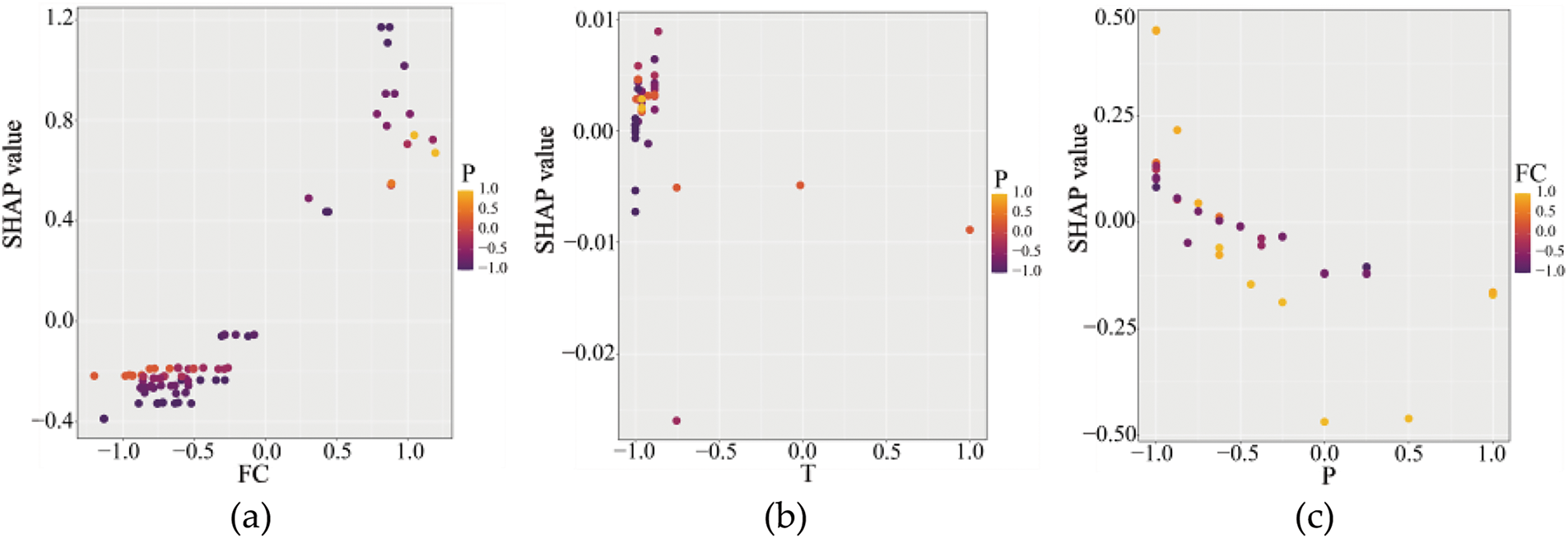
Figure 14: SHAP dependence plots for the SSA-XGBoost model: (a) FC & P; (b) T & P; (c) P & FC

Fig. 14b illustrates the relationship between parameter T and its SHAP values, with the color representing the values of parameter P. The plot reveals that most SHAP values are close to zero, indicating that T has a minimal influence on the model output. Additionally, the color gradient, ranging from purple (low values) to yellow (high values), represents the values of P. The distribution of colors appears uniform, suggesting that P does not significantly modulate the SHAP values of T. This indicates no notable interaction between P and T in the model.

Fig. 14c illustrates the relationship between parameter P and its SHAP values, with color indicating the values of parameter FC. Firstly, the plot reveals a negative correlation between P and SHAP values. Additionally, the color gradient, representing FC values, provides further insights. When the P value is low, the increase in the FC value leads to a more pronounced increase in the SHAP value, thereby exerting a stronger positive influence on the model output.

In conclusion, we can draw the following conclusions by SHAP: (1) Parameter FC has a significant positive effect on model output. At the same time, there is a significant interaction effect between P and FC. When FC is high or low, and P is low, the predicted output of the model will be significantly pushed up or down. (2) Parameter T has little influence on model output, is not an important driver of model prediction, and has no significant interaction with parameter P. (3) The value of parameter P has a negative effect on model output. When a lower P value is combined with a larger FC value, the SHAP value will be significantly increased, indicating that they have an interactive influence on the model within a specific value range.

The SSA-XGBoost model was explained using PDP and ICE interpretation techniques, implemented via the VIVID model interpretation package in R [73]. The results are presented in Fig. 15. First, Fig. 15a provides an overall parameter interpretation, including the importance ranking of individual parameters (Vimp) and the importance ranking of parameter combinations (Vint). The color gradient, ranging from light to dark, indicates the level of importance from low to high. The rank of individual importance of the input parameter is FC, P, and T, while the combination importance ranking is FC & P, FC & T, and P & T. We then move on to the heterogeneous effects that the three parameters, FC, P, and T, exert on the target variable. The ICE curves in the diagonals of Fig. 15b express how different parameters influence the prediction for any given instance; the diversity of their effects across instances may be captured there. In contrast, the top triangular section of the figure shows PDPs capturing the average impact of every parameter on the overall predictions.

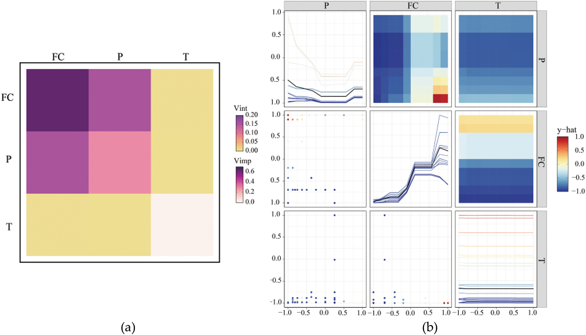
Figure 15: PDP and ICE-based interpretation of the SSA-XGBoost model: (a) importance ranking of Vimp and Vint; (b) PDPs and ICE curves

For the ICE curve of the parameter P, the resulting curves are smooth and quite similar across samples; this points to a strong and well-defined dependence of the model with respect to P. This would, therefore, indicate that the model effectively captures the relationship of P to the target variable. The ICE curve of FC is relatively very nonlinear, particularly for values of FC close to 0. Individual variation of these curves shows that FC has a different effect across samples; this could be because of feature interactions or local effects. This evidences the fact that the model can learn complex nonlinear relationships. For parameter T, the corresponding ICE is almost flat, reflecting that it has a very limited influence on the model’s predictions on this dataset. In general, the produced ICE curves have shown an excellent level of smoothness and coherence among the main parameters, such as P, underlying the fact that the proposed SSA-XGBoost model provides stable and reliable responses to critical features. At the same time, the model demonstrates flexibility in capturing nonlinear relationships in more complex features like FC, making it well-suited to handling diverse data distributions.

The PDP analysis provides additional insights into feature interactions. The PDP plot for P and FC shows strong color gradients, particularly when FC approaches 1, where predictions turn distinctly red, indicating a substantial increase. This reflects a significant interaction effect, where high FC values amplify the impact of P on predictions. The interaction between FC and T is weaker, as evidenced by a moderate color gradient, suggesting that FC’s influence is only slightly modulated by T, which aligns with the conclusion that T is not a critical variable. For P and T, the nearly flat color gradient indicates their combination has a negligible effect on predictions, further supporting T’s minimal importance and the lack of a significant dependency between P and T. Overall, the model demonstrates high sensitivity to the interaction between P and FC, moderate sensitivity to FC and T interactions, and low sensitivity to variations in T, consistent with prior ICE curve analysis.

7  Conclusions

This study successfully integrated advanced ML algorithms and GEP techniques to predict CO2-induced alterations in coal strength accurately. A total of six models were developed, including the GWO-XGBoost, SSA-XGBoost, and PO-XGBoost models, as well as the GEP-1, GEP-2, and GEP-3 models. A MATLAB-based application (APP) was developed to enhance the practical applicability of the model in engineering applications. In addition, by incorporating three model interpretability techniques, the study provided a comprehensive explanation of the best-performing model (SSA-XGBoost model), uncovering the unique contributions of each parameter to coal strength. The key conclusions are as follows:

(1) The MH-XGBoost models and GEP models demonstrated remarkable predictive performance.

(2) Non-parametric test results showed that the GWO-XGBoost, SSA-XGBoost, and PO-XGBoost models, along with the GEP-1 model, significantly outperformed the GEP-2 and GEP-3 models.

(3) The innovative indicator (D-GPI) identified the SSA-XGBoost model as the best-performing model, achieving exceptional predictive accuracy and reliability with an R² of 0.99396, RMSE of 0.62102, MAE of 0.36164, MAPE of 4.8101%, and RPD of 13.4741.

(4) A MATLAB-based application was developed to provide real-time predictions of coal strength changes, featuring a user-friendly interface to support research and industrial decision-making.

(5) SHAP-based interpretability analysis revealed that parameter FC had a significant positive effect on model output, while parameter P exerted a negative effect. A strong interaction effect was observed between P and FC, whereas parameter T had minimal influence on model output.

(6) ICE-based analysis demonstrated that the SSA-XGBoost model provided stable and reliable responses to critical features. Additionally, the model showed flexibility in capturing nonlinear relationships in complex features like FC, making it suitable for handling diverse data distributions.

(7) PDP-based analysis indicated that the model exhibited high sensitivity to the interaction between P and FC, moderate sensitivity to interactions between FC and T, and low sensitivity to variations in T.

Overall, the proposed models effectively address the task of CO2-induced strength prediction. The outstanding results of this study also confirm the application potential of the MH-XGBoost model, or more broadly, ML techniques, and GEP technology in strength prediction. Furthermore, the MH-XGBoost models we adopted demonstrates significant flexibility. Future studies may explore adapting these models to other materials or environmental conditions, thus expanding their application beyond coal strength prediction. For example, the models could be expanded by incorporating the properties of other materials, such as moisture content, porosity, and mineral composition, and their relationship to strength, to extend to other types of rocks, cement, or synthetic materials. This study’s primary limitation lies in the dataset’s scope, which may affect the model’s generalization ability. Therefore, future research should focus on expanding the applicability of these models to various coal types and geological conditions with further experiments. This includes incorporating additional influencing parameters and increasing dataset size to enhance model robustness and generalizability.

Acknowledgement: We thank the National Natural Science Foundation of China (42177164, 52474121) and the Outstanding Youth Project of Hunan Provincial Department of Education (23B0008) for their support of this study.

Funding Statement: This research is partially supported by the National Natural Science Foundation of China (42177164, 52474121) and the Outstanding Youth Project of Hunan Provincial Department of Education (23B0008).

Author Contributions: Zijian Liu: Methodology, Formal analysis, Validation, Resources, Visualization, Software, Writing—original draft. Yong Shi: Formal analysis, Visualization, Investigation, Writing—review & editing. Chuanqi Li: Formal analysis, Writing—review & editing. Xiliang Zhang: Formal analysis, Visualization, Investigation, Writing—review & editing, Supervision. Manoj Khandelwal: Formal analysis, Investigation, Writing—review & editing. Jian Zhou: Conceptualization, Methodology, Validation, Investigation, Visualization, Writing—review & editing, Supervision, Funding acquisition. All authors reviewed the results and approved the final version of the manuscript.

Availability of Data and Materials: The code used in this study, as well as the details of the database, are available on GitHub: https://github.com/CSUlzj/CO2-Induced-Alterations-in-Coal-Strength.git (accessed on 17 February 2025).

Ethics Approval: Not applicable.

Conflicts of Interest: The authors declare no conflicts of interest to report regarding the present study.

References

1. Florides GA, Christodoulides P. Global warming and carbon dioxide through sciences. Environ Int. 2009;35:390–401. doi:10.1016/j.envint.2008.07.007. [Google Scholar] [PubMed] [CrossRef]

2. Bagga P, Roy DG, Singh TN. Effect of carbon dioxide sequestration on the mechanical properties of Indian coal. In: ISRM EUROCK & 64th Geomechanics Colloquium-Future Development of Rock Mechanics; 2015; Salzburg, Austria. p. 1163–8. [Google Scholar]

3. Araújo ODQF, de Medeiros JL. Carbon capture and storage technologies: present scenario and drivers of innovation. Curr Opin Chem Eng. 2017;17:22–34. doi:10.1016/j.coche.2017.05.004. [Google Scholar] [CrossRef]

4. Leung DY, Caramanna G, Maroto-Valer MM. An overview of current status of carbon dioxide capture and storage technologies. Renew Sustain Energ Rev. 2014;39:426–43. doi:10.1016/j.rser.2014.07.093. [Google Scholar] [CrossRef]

5. Stevens SH, Kuuskraa VA, Gale J, Beecy D. CO2 injection and sequestration in depleted oil and gas fields and deep coal seams: worldwide potential and costs. Environ Geosci. 2001;8:200–9. doi:10.1046/j.1526-0984.2001.008003200.x. [Google Scholar] [CrossRef]

6. Li Z, Dong M, Li S, Huang S. CO2 sequestration in depleted oil and gas reservoirs—caprock characterization and storage capacity. Energy Convers Manag. 2006;47:1372–82. doi:10.1016/j.enconman.2005.08.023. [Google Scholar] [CrossRef]

7. Gale J, Freund P. Coal-bed methane enhancement with CO2 sequestration worldwide potential. Environ Geosci. 2001;8:210–7. doi:10.1046/j.1526-0984.2001.008003210.x. [Google Scholar] [CrossRef]

8. Omotilewa OJ, Panja P, Vega-Ortiz C, McLennan J. Evaluation of enhanced coalbed methane recovery and carbon dioxide sequestration potential in high volatile bituminous coal. J Nat Gas Sci Eng. 2021;91:103979. doi:10.1016/j.jngse.2021.103979. [Google Scholar] [CrossRef]

9. Perera MSA, Ranjith P, Viete DR. Effects of gaseous and super-critical carbon dioxide saturation on the mechanical properties of bituminous coal from the Southern Sydney Basin. Appl Energy. 2013;110:73–81. doi:10.1016/j.apenergy.2013.03.069. [Google Scholar] [CrossRef]

10. Ettinger I, Lamba E. Gas medium in coal-breaking processes. Fuel. 1957;36:298–306. [Google Scholar]

11. Czapliński A, Hołda S. Changes in mechanical properties of coal due to sorption of carbon dioxide vapour. Fuel. 1982;61:1281–2. [Google Scholar]

12. Holda S. Investigation of adsorption, dilatometry and strength of low rank coal. Archiwum Gornictwa. 1986;31:599–608. [Google Scholar]

13. Ateş Y. The effect of sorption on strength of coal and its influence on coal outbursts [master’s thesis]. Edmonton, AB, Canada: The University of Alberta; 1987. [Google Scholar]

14. Ates Y, Barron K. The effect of gas sorption on the strength of coal. Min Sci Technol. 1988;6:291–300. doi:10.1016/S0167-9031(88)90287-3. [Google Scholar] [CrossRef]

15. Chaback J, Morgan W, Yee D. Sorption of nitrogen, methane, carbon dioxide and their mixtures on bituminous coals at in-situ conditions. Fluid Phase Equilib. 1996;117:289–96. doi:10.1016/0378-3812(95)02965-6. [Google Scholar] [CrossRef]

16. Aziz N, Ming-Li W. The effect of sorbed gas on the strength of coal—an experimental study. Geotech Geolog Eng. 1999;17:387–402. doi:10.1023/A:1008995001637. [Google Scholar] [CrossRef]

17. Viete DR, Ranjith PG. The effect of CO2 on the geomechanical and permeability behaviour of brown coal: implications for coal seam CO2 sequestration. Int J Coal Geol. 2006;66:204–16. doi:10.1016/j.coal.2005.09.002. [Google Scholar] [CrossRef]

18. Ranathunga A, Perera M, Ranjith P. Influence of CO2 adsorption on the strength and elastic modulus of low rank Australian coal under confining pressure. Int J Coal Geol. 2016;167:148–56. doi:10.1016/j.coal.2016.08.027. [Google Scholar] [CrossRef]

19. Ranathunga AS, Perera MSA, Ranjith P, Bui H. Super-critical CO2 saturation-induced mechanical property alterations in low rank coal: an experimental study. J Supercrit Fluids. 2016;109:134–40. doi:10.1016/j.supflu.2015.11.010. [Google Scholar] [CrossRef]

20. Roy DG, Singh T. Predicting deformational properties of Indian coal: soft computing and regression analysis approach. Measurement. 2020;149:106975. doi:10.1016/j.measurement.2019.106975. [Google Scholar] [CrossRef]

21. Zhang P, Wang J, Jiang L, Zhou T, Yan X, Yuan L, et al. Influence analysis and stepwise regression of coal mechanical parameters on uniaxial compressive strength based on orthogonal testing method. Energies. 2020;13(14):3640. doi:10.3390/en13143640. [Google Scholar] [CrossRef]

22. Sampath K, Perera M, Ranjith P, Matthai S, Tao X, Wu B. Application of neural networks and fuzzy systems for the intelligent prediction of CO2-induced strength alteration of coal. Measurement. 2019;135:47–60. doi:10.1016/j.measurement.2018.11.031. [Google Scholar] [CrossRef]

23. Qiu Y, Zhou J. Methodology for constructing explicit stability formulas for hard rock pillars: integrating data-driven approaches and interpretability techniques. Rock Mech Rock Eng. 2025;11(22):1–28. doi:10.1007/s00603-025-04387-x. [Google Scholar] [CrossRef]

24. Huang S, Zhou J. Refined approaches for open stope stability analysis in mining environments: hybrid SVM model with multi-optimization strategies and GP technique. Rock Mech Rock Eng. 2024;57(11):9781–804. doi:10.1007/s00603-024-04055-6. [Google Scholar] [CrossRef]

25. Li C, Mei X, Zhang J. Application of supervised random forest paradigms based on optimization and post-hoc explanation in underground stope stability prediction. Appl Soft Comput. 2024;154:111388. doi:10.1016/j.asoc.2024.111388. [Google Scholar] [CrossRef]

26. Momeni E, Armaghani DJ, Hajihassani M, Amin MFM. Prediction of uniaxial compressive strength of rock samples using hybrid particle swarm optimization-based artificial neural networks. Measurement. 2015;60:50–63. doi:10.1016/j.measurement.2014.09.075. [Google Scholar] [CrossRef]

27. Yan H, Zhang J, Zhou N, Li M. Application of hybrid artificial intelligence model to predict coal strength alteration during CO2 geological sequestration in coal seams. Sci Total Environ. 2020;711:135029. doi:10.1016/j.scitotenv.2019.135029. [Google Scholar] [PubMed] [CrossRef]

28. Jahed Armaghani D, Tonnizam Mohamad E, Momeni E, Narayanasamy MS, Mohd Amin MF. An adaptive neuro-fuzzy inference system for predicting unconfined compressive strength and Young’s modulus: a study on Main Range granite. Bull Eng Geol Environ. 2015;74(4):1301–19. doi:10.1007/s10064-014-0687-4. [Google Scholar] [CrossRef]

29. Chen T, Guestrin C. XGBoost: a scalable tree boosting system. In: Proceedings of the 22nd ACM SIGKDD International Conference on Knowledge Discovery and Data Mining; 2016; San Francisco, CA, USA. [Google Scholar]

30. Cao J, Gao J, Nikafshan Rad H, Mohammed AS, Hasanipanah M, Zhou J. A novel systematic and evolved approach based on XGBoost-firefly algorithm to predict Young’s modulus and unconfined compressive strength of rock. Eng Comput. 2022;38(S5):3829–45. doi:10.1007/s00366-020-01241-2. [Google Scholar] [CrossRef]

31. Qiu Y, Zhou J, Khandelwal M, Yang H, Yang P, Li C. Performance evaluation of hybrid WOA-XGBoost, GWO-XGBoost and BO-XGBoost models to predict blast-induced ground vibration. Eng Comput. 2022;38(S5):4145–62. doi:10.1007/s00366-021-01393-9. [Google Scholar] [CrossRef]

32. Mirjalili S, Mirjalili SM, Lewis A. Grey wolf optimizer. Adv Eng Softw. 2014;69:46–61. doi:10.1016/j.advengsoft.2013.12.007. [Google Scholar] [CrossRef]

33. Xue J, Shen B. A novel swarm intelligence optimization approach: sparrow search algorithm. Syst Sci Cont Eng. 2020;8(1):22–34. doi:10.1080/21642583.2019.1708830. [Google Scholar] [CrossRef]

34. Lian J, Hui G, Ma L, Zhu T, Wu X, Heidari AA, et al. Parrot optimizer: algorithm and applications to medical problems. Comput Biol Med. 2024;172(5):108064. doi:10.1016/j.compbiomed.2024.108064. [Google Scholar] [PubMed] [CrossRef]

35. Zareian L, Rahebi J, Shayegan MJ. Bitterling fish optimization (BFO) algorithm. Multimed Tools Appl. 2024;83(31):1–34. doi:10.1007/s11042-024-18579-0. [Google Scholar] [CrossRef]

36. Amiri MH, Mehrabi Hashjin N, Montazeri M, Mirjalili S, Khodadadi N. Hippopotamus optimization algorithm: a novel nature-inspired optimization algorithm. Sci Rep. 2024;14(1):5032. doi:10.1038/s41598-024-54910-3. [Google Scholar] [PubMed] [CrossRef]

37. Abdollahzadeh B, Gharehchopogh FS, Khodadadi N, Mirjalili S. Mountain gazelle optimizer: a new nature-inspired metaheuristic algorithm for global optimization problems. Adv Eng Softw. 2022;174(3):103282. doi:10.1016/j.advengsoft.2022.103282. [Google Scholar] [CrossRef]

38. Rao R. Rao algorithms: three metaphor-less simple algorithms for solving optimization problems. Int J Ind Eng Comput. 2020;11(1):107–30. doi:10.5267/j.ijiec.2019.6.002. [Google Scholar] [CrossRef]

39. Kennedy J, Eberhart R. Particle swarm optimization. In: Proceedings of ICNN’95-International Conference on Neural Networks; 1995; Perth, WA, Australia. Vol. 4, p. 1942–8. [Google Scholar]

40. Holland JH. Genetic algorithms. Sci Am. 1992;267(1):66–73. doi:10.1038/scientificamerican0792-66. [Google Scholar] [CrossRef]

41. Li C, Zhou J, Du K, Dias D. Stability prediction of hard rock pillar using support vector machine optimized by three metaheuristic algorithms. Int J Min Sci Technol. 2023;33(8):1019–36. doi:10.1016/j.ijmst.2023.06.001. [Google Scholar] [CrossRef]

42. Zhou J, Huang S, Qiu Y. Optimization of random forest through the use of MVO, GWO and MFO in evaluating the stability of underground entry-type excavations. Tunnelling Undergr Space Technol. 2022;124(12):104494. doi:10.1016/j.tust.2022.104494. [Google Scholar] [CrossRef]

43. Zhou J, Huang S, Wang M, Qiu Y. Performance evaluation of hybrid GA-SVM and GWO-SVM models to predict earthquake-induced liquefaction potential of soil: a multi-dataset investigation. Eng Comput. 2022;38(S5):1–19. doi:10.1007/s00366-021-01418-3. [Google Scholar] [CrossRef]

44. Zhou J, Wang Z, Qiu Y, Li P, Tao M. Sparrow search algorithm enhanced multi-output regression for predicting rock fracture shear displacements: a metaheuristic-hybridized model. Mech Adv Mater Struct. 2024;85:1–17. doi:10.1080/15376494.2024.2361859. [Google Scholar] [CrossRef]

45. Zhou J, Dai Y, Huang S, Armaghani DJ, Qiu Y. Proposing several hybrid SSA—machine learning techniques for estimating rock cuttability by conical pick with relieved cutting modes. Acta Geotechnica. 2023;18(3):1431–46. doi:10.1007/s11440-022-01685-4. [Google Scholar] [CrossRef]

46. Ferreira C. Gene expression programming: a new adaptive algorithm for solving problems. arXiv:cs/0102027. 2001. [Google Scholar]

47. Ahmad A, Chaiyasarn K, Farooq F, Ahmad W, Suparp S, Aslam F. Compressive strength prediction via gene expression programming (GEP) and artificial neural network (ANN) for concrete containing RCA. Buildings. 2021;11(8):324. doi:10.3390/buildings11080324. [Google Scholar] [CrossRef]

48. Zhou J, Zhang R, Qiu Y, Khandelwal M. A true triaxial strength criterion for rocks by gene expression programming. J Rock Mech Geotechnical Eng. 2023;15(10):2508–20. doi:10.1016/j.jrmge.2023.03.004. [Google Scholar] [CrossRef]

49. Van den Broeck G, Lykov A, Schleich M, Suciu D. On the tractability of SHAP explanations. J Artif Intell Res. 2022;74:851–86. doi:10.1613/jair.1.13283. [Google Scholar] [CrossRef]

50. Xi B, Li E, Fissha Y, Zhou J, Segarra P. LGBM-based modeling scenarios to compressive strength of recycled aggregate concrete with SHAP analysis. Mech Adv Mater Struct. 2024;31(23):5999–6014. doi:10.1080/15376494.2023.2224782. [Google Scholar] [CrossRef]

51. Johnson PM, Barbour W, Camp JV, Baroud H. Using machine learning to examine freight network spatial vulnerabilities to disasters: a new take on partial dependence plots. Transport Res Interdiscip Perspect. 2022;14(1):100617. doi:10.1016/j.trip.2022.100617. [Google Scholar] [CrossRef]

52. Nagelkerke NJ. A note on a general definition of the coefficient of determination. biometrika. 1991;78(3):691–2. doi:10.1093/biomet/78.3.691. [Google Scholar] [CrossRef]

53. Vasques G, Grunwald S, Sickman J. Comparison of multivariate methods for inferential modeling of soil carbon using visible/near-infrared spectra. Geoderma. 2008;146(1–2):14–25. doi:10.1016/j.geoderma.2008.04.007. [Google Scholar] [CrossRef]

54. Chai T, Draxler RR. Root mean square error (RMSE) or mean absolute error (MAE)?—arguments against avoiding RMSE in the literature. Geosci Model Dev. 2014;7(3):1247–50. doi:10.5194/gmd-7-1247-2014. [Google Scholar] [CrossRef]

55. Perera M, Ranjith P, Peter M. Effects of saturation medium and pressure on strength parameters of Latrobe Valley brown coal: carbon dioxide, water and nitrogen saturations. Energy. 2011;36:6941–7. doi:10.1016/j.energy.2011.09.026. [Google Scholar] [CrossRef]

56. Wang Q, Zhang D, Wang H, Jiang W, Wu X, Yang J, et al. Influence of CO2 exposure on high-pressure methane and CO2 adsorption on various rank coals: implications for CO2 sequestration in coal seams. Ener Fuels. 2015;29:3785–95. doi:10.1021/acs.energyfuels.5b00058. [Google Scholar] [CrossRef]

57. Sampath K, Ranjith P, Perera M. A comprehensive review of structural alterations in CO2-interacted coal: insights into CO2 sequestration in coal. Ener Fuels. 2020;34:13369–83. doi:10.1021/acs.energyfuels.0c02782. [Google Scholar] [CrossRef]

58. Uribe CA, Pérez FH. Proposal for coal classification. Fuel. 1985;64(2):147–50. doi:10.1016/0016-2361(85)90207-8. [Google Scholar] [CrossRef]

59. Perera M, Ranjith P, Choi S, Bouazza A, Kodikara J, Airey D. A review of coal properties pertinent to carbon dioxide sequestration in coal seams: with special reference to Victorian brown coals. Environ Earth Sci. 2011;64:223–35. doi:10.1007/s12665-010-0841-7. [Google Scholar] [CrossRef]

60. Zhi S, Elsworth D, Liu L. W-shaped permeability evolution of coal with supercritical CO2 phase transition. Int J Coal Geol. 2019;211:103221. doi:10.1016/j.coal.2019.103221. [Google Scholar] [CrossRef]

61. Liu X, Jia X, Niu Y, Nie B, Zhang C, Song D. Alterations in coal mechanical properties and permeability influenced by liquid CO2 phase change fracturing. Fuel. 2023;354:129254. doi:10.1016/j.fuel.2023.129254. [Google Scholar] [CrossRef]

62. Wang K, Ma L, Taylor KG. Microstructure changes as a response to CO2 storage in sedimentary rocks: recent developments and future challenges. Fuel. 2023;333:126403. doi:10.1016/j.fuel.2022.126403. [Google Scholar] [CrossRef]

63. Talu O. Needs, status, techniques and problems with binary gas adsorption experiments. Adv Colloid Interface Sci. 1998;76:227–69. doi:10.1016/S0001-8686(98)00048-7. [Google Scholar] [CrossRef]

64. Ranjith P, Perera MSA. Effects of cleat performance on strength reduction of coal in CO2 sequestration. Energy. 2012;45:1069–75. doi:10.1016/j.energy.2012.05.041. [Google Scholar] [CrossRef]

65. Ranjith P, Jasinge D, Choi S, Mehic M, Shannon B. The effect of CO2 saturation on mechanical properties of Australian black coal using acoustic emission. Fuel. 2010;89:2110–7. doi:10.1016/j.fuel.2010.03.025. [Google Scholar] [CrossRef]

66. Kattan MW, Cooper RB. A simulation of factors affecting machine learning techniques: an examination of partitioning and class proportions. Omega. 2000;28:501–12. doi:10.1016/S0305-0483(00)00015-3. [Google Scholar] [CrossRef]

67. Qiu Y, Zhou J, He B, Armaghani DJ, Huang S, He X. Evaluation and interpretation of blasting-induced tunnel overbreak: using heuristic-based ensemble learning and gene expression programming techniques. Rock Mech Rock Eng. 2024;57:7535–63. doi:10.1007/s00603-024-03947-x. [Google Scholar] [CrossRef]

68. Derrac J, García S, Molina D, Herrera F. A practical tutorial on the use of nonparametric statistical tests as a methodology for comparing evolutionary and swarm intelligence algorithms. Swarm Evol Comput. 2011;1:3–18. doi:10.1016/j.swevo.2011.02.002. [Google Scholar] [CrossRef]

69. Qiu Y, Zhou J. Short-term rockburst damage assessment in burst-prone mines: an explainable XGBOOST hybrid model with SCSO algorithm. Rock Mech Rock Eng. 2023;56(12):8745–70. doi:10.1007/s00603-023-03522-w. [Google Scholar] [CrossRef]

70. Qiu Y, Zhou J. Short-term rockburst prediction in underground project: insights from an explainable and interpretable ensemble learning model. Acta Geotechnica. 2023;18(12):6655–85. doi:10.1007/s11440-023-01988-0. [Google Scholar] [CrossRef]

71. Guidotti R, Monreale A, Ruggieri S, Turini F, Giannotti F, Pedreschi D. A survey of methods for explaining black box models. ACM Comput Surv. 2018;51:1–42. doi:10.1145/323600. [Google Scholar] [CrossRef]

72. Rudin C. Stop explaining black box machine learning models for high stakes decisions and use interpretable models instead. Nature Mach Intell. 2019;1(5):206–15. doi:10.1038/s42256-019-0048-x. [Google Scholar] [PubMed] [CrossRef]

73. Inglis A, Parnell A, Hurley C. vivid: an R package for variable importance and variable interactions displays for machine learning models. arXiv:2210.11391. 2022. [Google Scholar]