
 Submit a Paper
 Propose a Special lssue
 Open Access
ARTICLE

A Numerical Study of the Caputo Fractional Nonlinear Rössler Attractor Model via Ultraspherical Wavelets Approach
1 Department of Mathematics, School of Applied and Life Sciences, Uttaranchal University, Dehradun, 248007, India
2 Department of Mathematics, Saveetha School of Engineering, Saveetha Institute of Medical and Technical Sciences, Saveetha University, Chennai, 602105, India
3 Department of Mathematics, Radfan University College, University of Lahej, Lahej, 73560, Yemen
4 Department of Mathematics, College of Science, Korea University, Seoul, 02814, Republic of Korea
5 Department of Mathematics, College of Science and Humanities in Al-Kharj, Prince Sattam bin Abdulaziz University, Al-Kharj, 11942, Saudi Arabia
6 Faculty of Exact and Natural Sciences, School of Physical Sciences and Mathematics, Pontifical Catholic University of Ecuador, Sede Quito, 17-01-2184, Ecuador
* Corresponding Authors: Sabri T. M. Thabet. Email: ; Miguel Vivas-Cortez. Email:
(This article belongs to the Special Issue: Analytical and Numerical Solution of the Fractional Differential Equation)
Computer Modeling in Engineering & Sciences 2025, 143(2), 1895-1925. https://doi.org/10.32604/cmes.2025.060989
Received 14 November 2024; Accepted 27 January 2025; Issue published 30 May 2025
 View Full Text
 Download PDF
Abstract
The Rössler attractor model is an important model that provides valuable insights into the behavior of chaotic systems in real life and is applicable in understanding weather patterns, biological systems, and secure communications. So, this work aims to present the numerical performances of the nonlinear fractional Rössler attractor system under Caputo derivatives by designing the numerical framework based on Ultraspherical wavelets. The Caputo fractional Rössler attractor model is simulated into two categories, (i) Asymmetric and (ii) Symmetric. The Ultraspherical wavelets basis with suitable collocation grids is implemented for comprehensive error analysis in the solutions of the Caputo fractional Rössler attractor model, depicting each computation in graphs and tables to analyze how fractional order affects the model’s dynamics. Approximate solutions obtained through the proposed scheme for integer order are well comparable with the fourth-order Runge-Kutta method. Also, the stability analyses of the considered model are discussed for different equilibrium points. Various fractional orders are considered while performing numerical simulations for the Caputo fractional Rössler attractor model by using Mathematica. The suggested approach can solve another non-linear fractional model due to its straightforward implementation.Keywords
In today’s world, accuracy is paramount across all fields, making the application of advanced mathematical techniques essential [1–4]. Fractional calculus (FC), an extension of traditional calculus, plays a crucial role in this regard [5–8]. Incorporating fractional derivatives and integrals, FC provides a strong framework for modeling complex systems with memory and inherited features, capturing phenomena that traditional models often overlook [9]. Its applications are increasingly widespread across various fields of science and engineering, offering new insights into real-world challenges. The reach of FC now extends into the areas such as robotics [10], stock market analysis [11], signal processing [12], chaotic dynamical systems [13], image processing [14], viscoelasticity [15], life sciences [16], neural networks [17], pharmacokinetic [18], and earthquake modeling [19]. This concept enhances the understanding and prediction of systems exhibiting non-local and time-dependent behavior.
Fractional operators [20–22] can be applied in any real or complex order, providing deeper analysis with the flexibility to approach dynamic systems. Fractional integrals generalize traditional integration to non-integer orders, using the Riemann-Liouville [23] or Caputo definitions [24,25]. Integral and differential operators are used in the Liouville and Riemann framework to investigate FC. The Caputo operator is a novel fractional operator that Caputo created, utilizing the framework of FC to study and analyze the models [26,27]. The Caputo fractional derivative is highly regarded as an efficient derivative for real-world applications, as it effectively incorporates initial and boundary conditions. Compared to other fractional derivatives like the Riemann-Liouville derivative, the Caputo derivative avoids certain mathematical complexities, such as needing non-local initial conditions that are more computationally challenging. The use of the Caputo derivative in real-world scenarios often leads to more accurate solutions than other derivatives, when combined with orthogonal polynomials and wavelet-based methods. By incorporating kernel functions that account for historical effects, they effectively model systems with long-range dependencies, such as anomalous diffusion and viscoelastic behavior [28]. Their ability to capture non-local interactions makes them invaluable in fields like physics [29], engineering [30,31], finance [32], and control theory [33] and provide essential tools for understanding complex phenomena. One such tool is a wavelet transform.
Wavelet Transform is a mathematical technique that deals with an expansion of functions as a basis function. Operations on wavelets form wavelets theory [34–36] which can be employed in various fields such as image analysis, control systems, communication systems, stock market analysis, a meteorological model, solutions to differential equations [37,38], and many others [39–41]. In recent years, the wavelets approach has become more and more popular in the areas of numerical methods. Several types of wavelets and function approximation were utilized in these references [42–44]. Wavelet-based approaches are employed for solving differential equations, particularly non-linear differential equations, providing highly accurate solutions by using integration to transform differential equations into integral equations [45–48]. The functions or signals associated with the equations are then compared using truncated orthogonal series expansions. The integral operations within these equations are eliminated by applying an operational matrix of integration, thereby effectively reducing the considered problem to a series of algebraic equations, and simplifying the calculation process. One of its applications includes analyzing chaotic dynamic systems.
Chaotic dynamical systems [49,50] are sensitive to the state of initial conditions applied to the systems. Its characteristics such as unpredictability, sensitivity to initial conditions, and complex dynamics play vital roles in solving real-world scenarios. They are crucial in understanding weather patterns [51], predicting population dynamics [52], encryption in cryptocurrency [53] encryption in image [54], and other fields. In the realm of chaos and dynamical systems, particularly for low-dimensional models, the Lorenz system [55] and Rössler model [56] are two seminal examples that have been widely examined. These models are fundamental in exploring and understanding chaotic dynamics and have contributed a significant role in the advancement of the related fields. The Lorenz system is more complex and closely associated with physical phenomena, generating a double-lobed butterfly attractor representing more intricate chaos. On the other hand, the Rössler system is simpler and serves as an abstract model of chaos, making it ideal for theoretical studies and easier visualizations. It produces a single spiral attractor, which reflects smoother chaos. The coexistence of both asymmetric and symmetric features in the Rössler system allows researchers to explore a broader spectrum of dynamical behaviors as compared to the asymmetric Lorenz system, making it a versatile and insightful model for studying chaotic dynamics. Due to these characteristics, a system of non-linear equation of Rössler attractor model is analyzed numerically in this study by using a wavelet-based technique.
The Rössler system [57] consists of three equations, being one non-linear, three system parameters
Model 1: Asymmetric fractional Rössler attractor [58]:
with the conditions
In contrast to the asymmetric Lorenz system, the Rössler system exhibits both symmetry and asymmetry characteristics. Asymmetric Rössler attractor is shown by the model given in Eq. (1). One can change the structure by making changes to the linear or nonlinear variables to build a symmetric system. A 180∘ rotation around the
Model 2: Symmetric fractional Rössler attractor [58]:
with the conditions
The operator
We will utilize the above two systems for our study under the conditions mentioned. Several researchers have studied the above models, their applications, and their nature by utilizing various methods and tools. In [59], Kontorovich et al. used the degenerated cumulant equations method for analysis and provided an application through Rössler attractor output signals to model radio frequency interferences provided by Peripheral Component Interface express. Rysak et al. [60] implemented the Grunwald-Letnikov method for numerical solutions of Caputo fractional Rössler attractor model and did a recurrence quantification analysis. In [61], Elbadri et al. presented a fractional Laplace decomposition technique with an adaptive predictor-corrector algorithm for solving rotationally symmetric Rössler attractor. Kekana et al. [62] conducted the analysis of Rössler attractor by residual and Joubert-Greeff methods. In [63], Barrio et al. studied the regions of parameters for chaotic behavior by using different chaos indicators and conducted a thorough analysis of the global and local bifurcations of co-dimension one and two of limit cycles. Santra et al. [64] provided the simulation of Rössler attractor through the power series approach. In [65], Boulehmi solved the Caputo fractional Rössler attractor model under the Atangana-Baleanu-Caputo fractional derivative and compared the results with the method.
In this study, we are interested in adapting a novel approach based on ultraspherical Wavelets (USWs) as basis functions for simulating Caputo fractional Rössler attractor model. These wavelets play a significant role in numerical analysis as well as in approximation theory. The importance of studying the fractional Rössler system lies in its potential for better analyzing the applications of such models. To the best of the author’s knowledge, this is the first time that the considered model under the Caputo derivative is numerically simulated using USWs. Therefore, motivated by the existing literature, the present work illustrates an application of USWs with collocation nodes to analyze the Caputo fractional Rössler attractor model under the Caputo derivative. An additional motivation is that the Legendre wavelets and Chebyshev wavelets can be inferred as particular instances of the USWs. The presented scheme does not appear to have any significant flaws. However, the suggested scheme works effectively in a limited domain, and processing a large number of USWs could lead to high computational costs. The novelty of this work is presented as:
• The Caputo fractional derivatives have been employed to get more accurate solutions to the Caputo fractional Rössler attractor model.
• The design of the computational framework based on USWs is presented for the first time to solve the Caputo fractional Rössler attractor model numerically.
• The relative representations have been presented through relative errors and
• A detailed error and equilibria analysis of the proposed model is provided in this study.
This work is organized as follows: Section 2 presents the fundamental ideas about fractional Caputo operators employed in this work. The USWs basis and approximation of function by USWs are described in Section 3. The USWs technique for simulating Caputo fractional Rössler attractor model is presented in Section 4. Section 5 provides the error and equilibria analysis. The nonlinear Caputo fractional Rössler attractor model is numerically analyzed in Section 6, showcasing results in tables and graphs that demonstrate the effectiveness of the suggested scheme. Section 7 contains the concluding remarks and the future scope.
Some preliminaries and notations about FC are included in this section. This work employs the following fractional operators.
Definition 2.1. The fractional Caputo derivative of a function
Definition 2.2. For a function
• For
3 Wavelets and Function Approximation
3.1 Brief Overview of Ultraspherical Wavelets
The USWs
The USWs are defined on [0, 1] as [67–69]
where
and
Here,
With respect to the weighted function
Let
An arbitrary function
where
If the given series in Eq. (10) is truncated, we obtain
where
In this study, we use
4 Solution of Caputo Fractional Rössler Attractor Model
In the present section, the Caputo fractional Rössler attractor model is solved by the USWs scheme with the collocation points. In this study, we selected the specific collocation points given in Eq. (25) because they are uniformly distributed over the interval, simplifying implementation and ensuring that the computational load is evenly distributed across the domain. Uniformly distributed points are particularly well-suited for our method, as they align well with the USWs framework, preserving the accuracy of the numerical solution for the fractional Rössler attractor model.
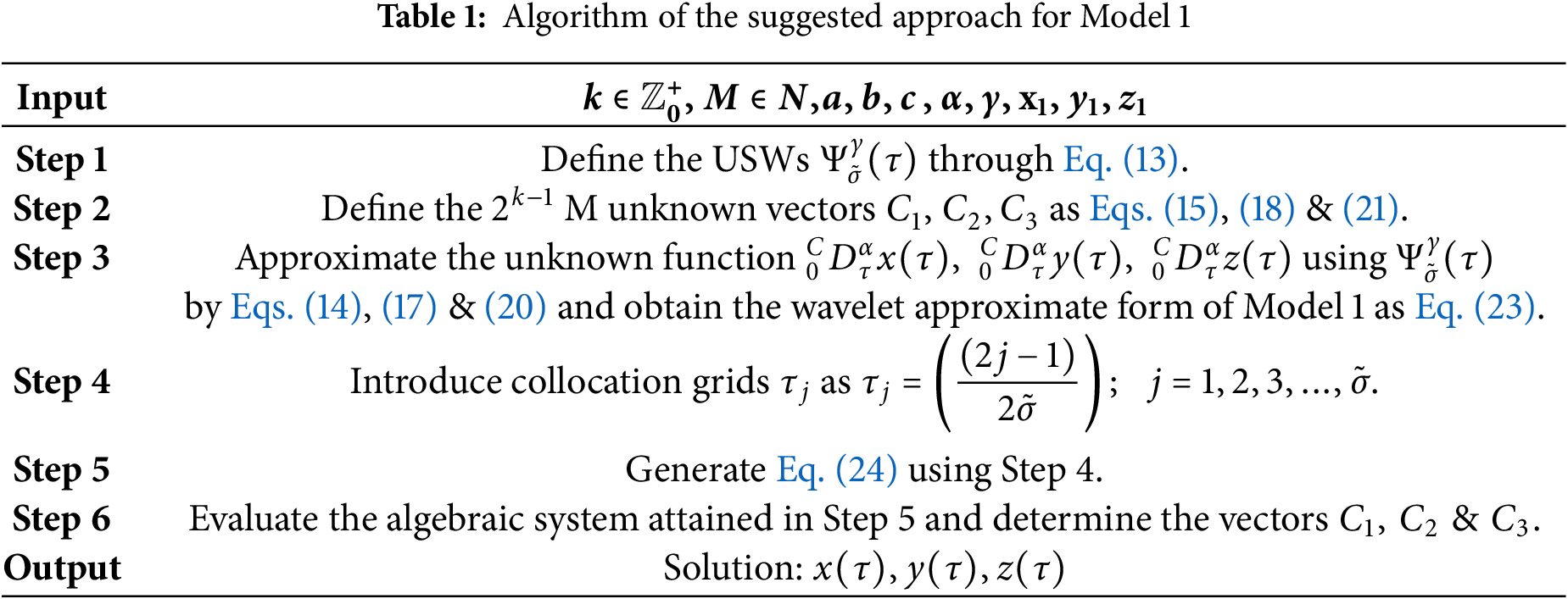
To evaluate the solutions of the Caputo fractional Rössler attractor model, the procedure of the described wavelets scheme is given as:
4.1 For Model 1 (Asymmetric Caputo Fractional Rössler Attractor Model)
Consider the asymmetric Caputo fractional Rössler attractor model given in Eq. (1) and provide the approximation for the unknown function
where
Taking the integral of Eq. (6) on Eq. (14), and using Eqs. (2) and (7), we get
where
Similarly, the unknown function
where wavelet coefficient
Taking integral of Eq. (6) on Eq. (17) and using Eqs. (2) and (7), we get
Similarly, the unknown term
where wavelet coefficient
Taking integral of Eq. (6) on Eq. (20) and using Eqs. (2) and (7), we get
Substituting Eqs. (14)–(22) in Eq. (1), we get the wavelet approximate form of Eq. (1) as
Collocating Eq. (23) at the collocation point
where
Solve the system of algebraic equations in Eq. (24) by Newton iteration method, we can readily obtain the wavelet coefficient vectors
The algorithm of the suggested approach for Model 1 is described in Table 1.
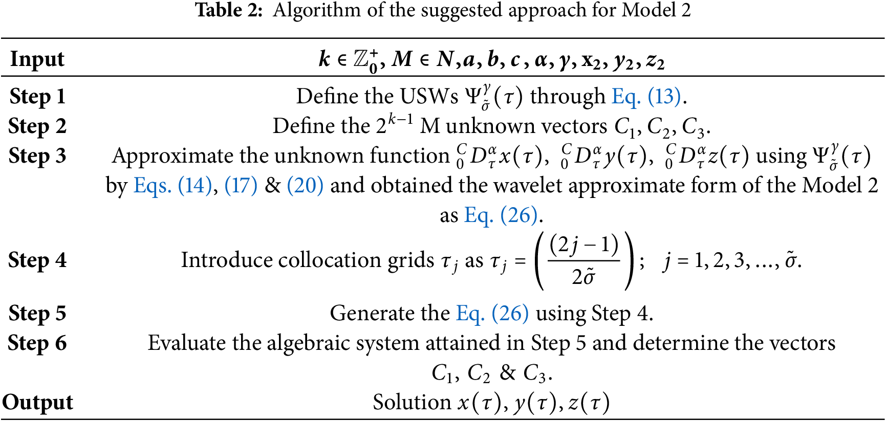
4.2 For Model 2 (Symmetric Caputo Fractional Rössler Attractor Model):
Express the unknown terms
Collocating Eq. (26) at the collocation point
where
Evaluate the algebraic system in Eq. (27) by Newton iteration method, we can readily obtain the wavelet coefficient vectors
The algorithm of the proposed approach for Model 2 is described in Table 2.
5 Error and Equilibria Analysis
This section first presents a detailed error analysis, followed by a comprehensive stability analysis of the Caputo fractional Rössler attractor model.
The residual error formula is presented for comparison purposes and to examine the efficacy of the described approach. The analytical solution of the considered model is not available for integer and non-integer order, therefore we provide a residual error function to assess the precision of the given scheme.
• For asymmetric fractional Rössler attractor, the residual error function is given as
where
• For symmetric fractional Rössler attractor, the residual error function is given as
• The maximum residual error (
• The minimum residual error (
• The
The fundamental findings corresponding to the approximation of Ultraspherical polynomials serve as the foundation for exploring the convergence of USWs approximations. The convergence of the series expansion of
Theorem 5.1. Consider the USWs expansion
where
Also,
where
Proof. For proof, see [68]. ▪
5.2 Existence and Uniqueness of Solution
Theorem 5.2 Every solution of the system (1) and (3) with positive initial values
Proof. For Model 1:
Let
Therefore, the system in (28) can be written in the form
For Model 2: Same proof as above. ▪
The solution of the Caputo fractional Rössler attractor model is overall assessed on the groundwork of steadiness points [64,65]. The steadiness points of the regarded model are attained by resolving the model under uniform state conditions. The examination of equilibrium points is split up into the eigenvalues signs. The Jacobian matrix of the model is constructed to analyze the signs of the eigenvalues to determine stability. Then, the behavior of the considered fractional model for each point of equilibrium can be subjectively evaluated by inspecting the nature of eigenvalues. When the Jacobian matrix has complex eigenvalues and the real part of the eigenvalues corresponding to the equilibrium points is positive, then the equilibrium points are the saddle spiral points. Also, if the Jacobian matrix has complex eigenvalues and positive real eigenvalues corresponding to the equilibrium points, then the equilibrium points are also saddle spiral points. The equilibrium points of the considered system will be asymptotically stable if all eigenvalues of the associated Jacobian matrix fulfill the Matignon condition [71]. The particular values of the parameters involved in the considered model are taken from [58].
For Model 1: The equilibrium points for asymmetric Caputo fractional Rössler attractor model are obtained as
i.e.,
The equilibrium points
where
Computing Jacobian MatrixJ for the considered Model 1 as
• The Jacobian Matrix at
The eigenvalues of
For
• The Jacobian Matrix at
The eigenvalues of
For
The discriminant of the characteristic equation of the Jacobian matrix corresponding to the equilibrium points
For Model 2: The equilibrium points for symmetric Caputo fractional Rössler attractor model are obtained as
i.e.,
By solving Eq. (31), we get the model’s equilibrium points.
The equilibrium points
where
Computing Jacobian Matrix J for the considered model as
• The Jacobian Matrix at
The eigenvalues for
For
• The Jacobian Matrix at
The eigenvalues for
For
• The Jacobian Matrix at
The eigenvalues for
For
The discriminant of the characteristic equation of the Jacobian matrix corresponding to the equilibrium points
6 Numerical Simulations and Discussion
The effectiveness and performance of the suggested approach are assessed by employing it in several cases, and the results are contrasted with existing systems that offer accurate solutions. In this study, both maximum and minimum residual errors are computed. Mentioning both residual errors provides a comprehensive view of model performance, and a clear range of errors, and allows for better assessment and comparison. All numerical results are obtained using Mathematica. All codes and figures in this study are executed and generated on the following kind of machine: Windows 10 Home operating system (64-bit), RAM of 8 GB, Intel Core i5-8250U CPU @ 1.60 GHz.
Now, both Caputo fractional Rössler attractor models are simulated for particular parameters [58] and their impact on the dynamics of the Caputo fractional Rössler attractor model.
6.1 Asymmetric Caputo Fractional Rössler Attractor Model
The asymmetric Caputo fractional Rössler attractor model is numerically simulated for
For this case, the Rössler model is represented through the following equations as
with the conditions
Since there is no solution and no comparison available for integer and non-integer order of this model, therefore we simulated this model for different
At
At
At
At
The estimated residual errors in the solution of asymmetric Caputo fractional Rössler attractor model for various values of
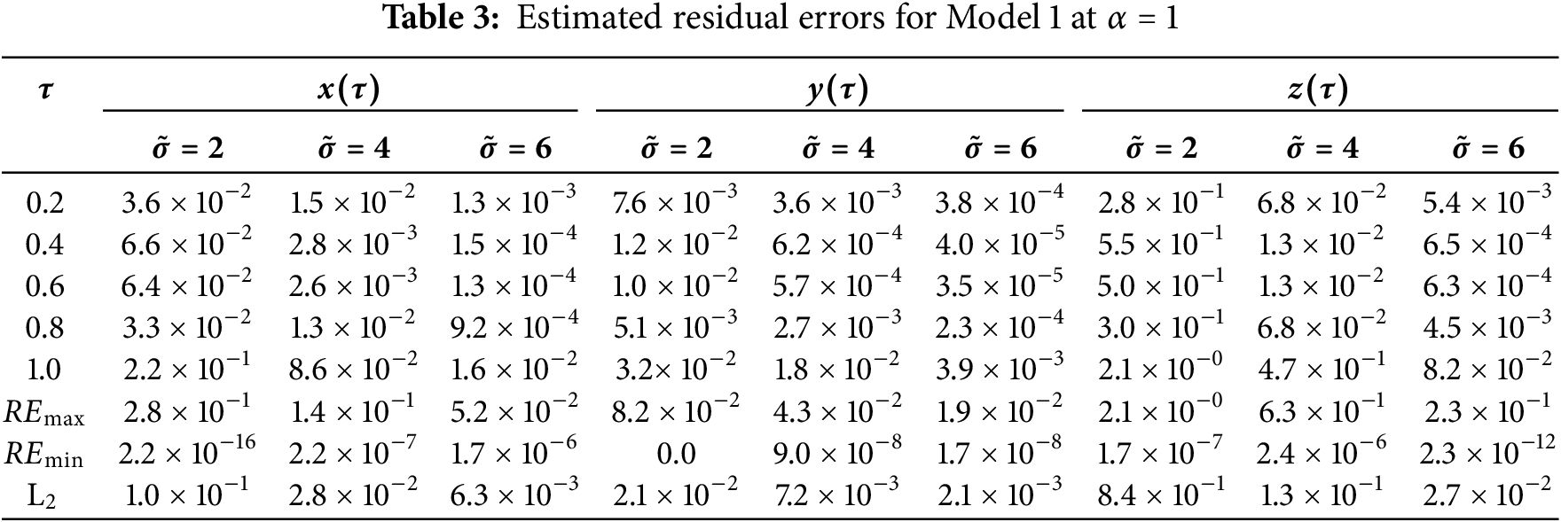
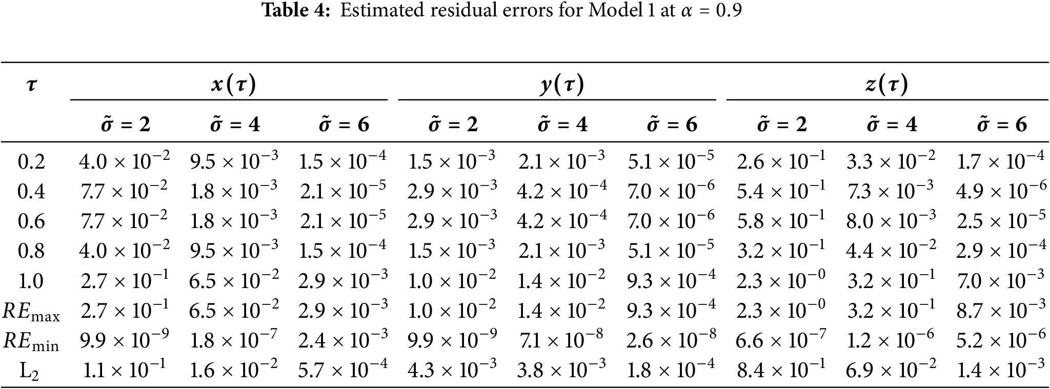

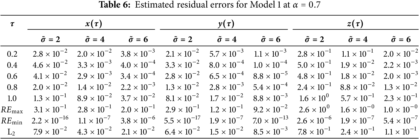
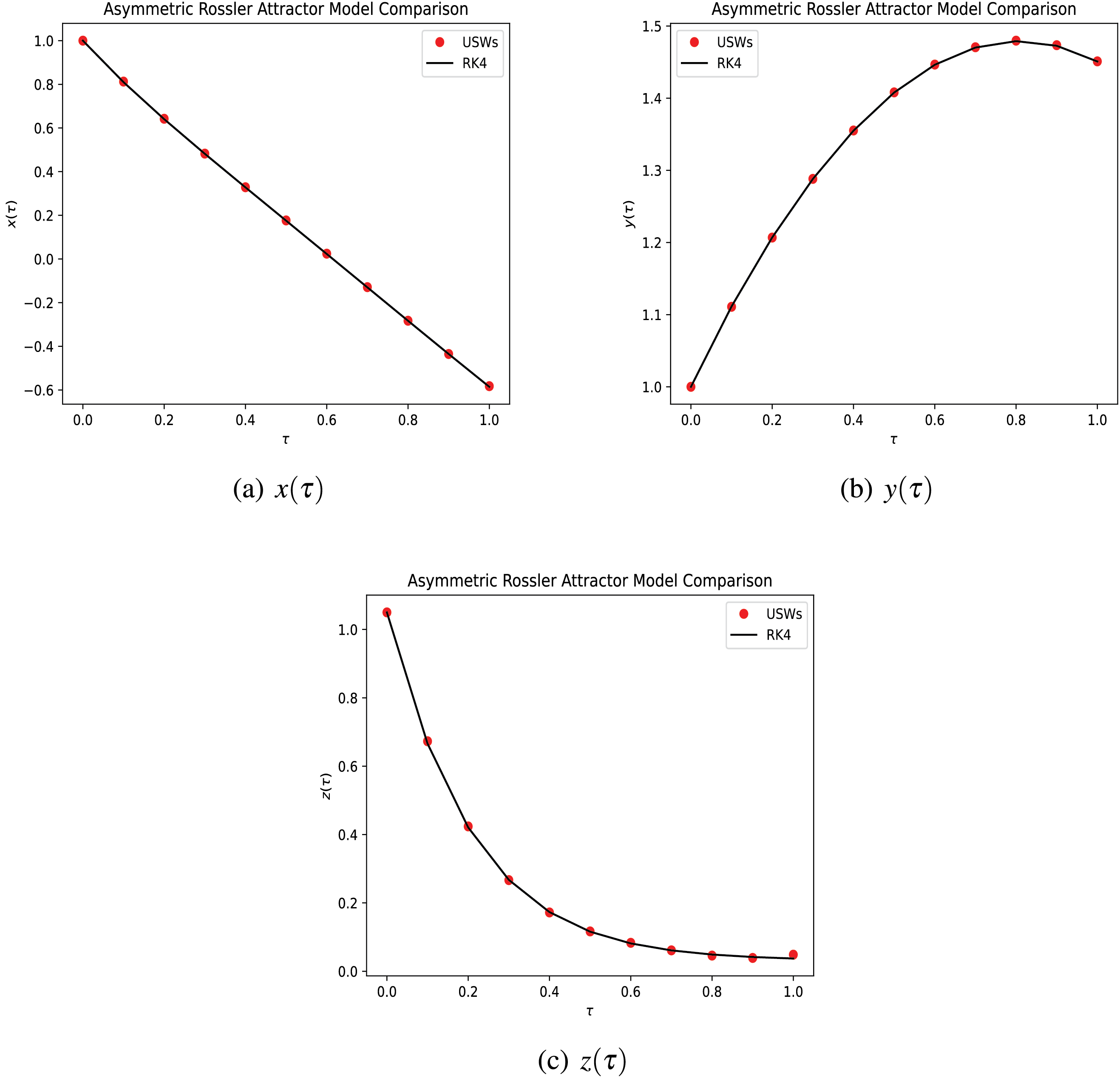
Figure 1: Solution of Model 1 via the suggested approach with fourth-order Range-Kutta method at
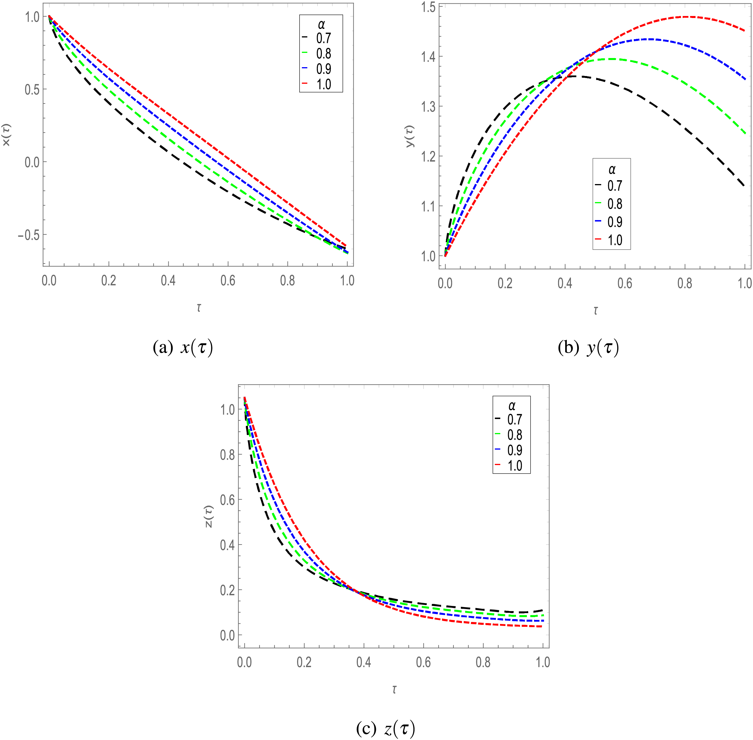
Figure 2: Solution of Model 1 for different
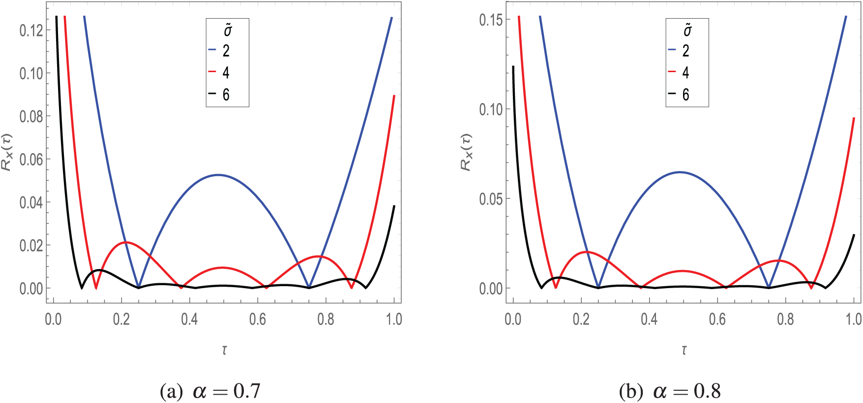
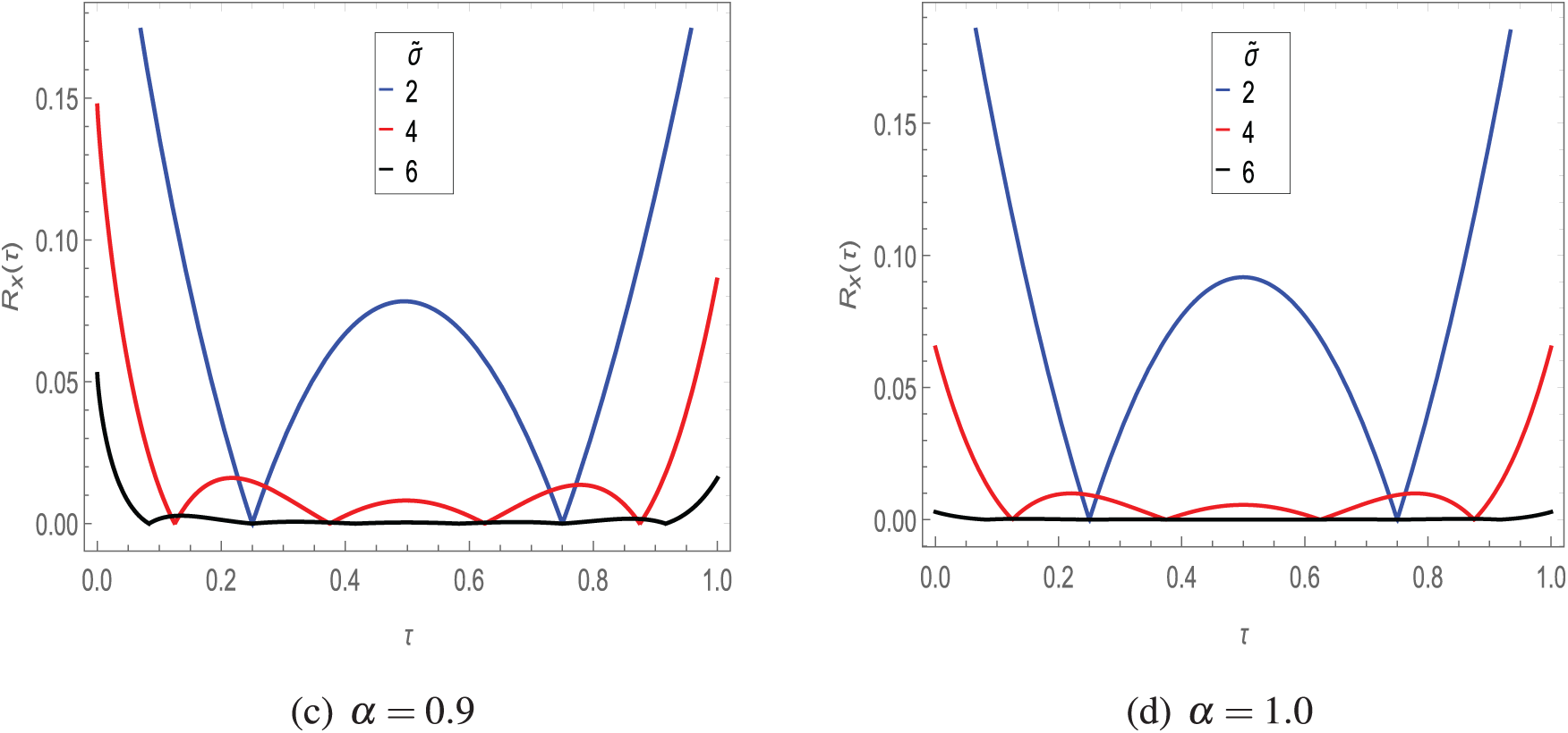
Figure 3: Residual error in
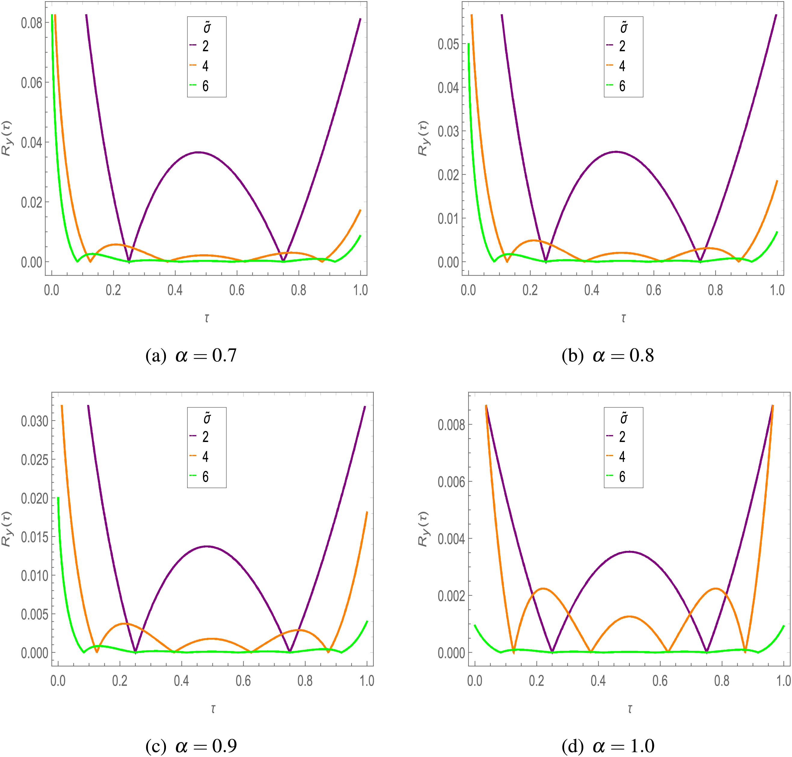
Figure 4: Residual error in
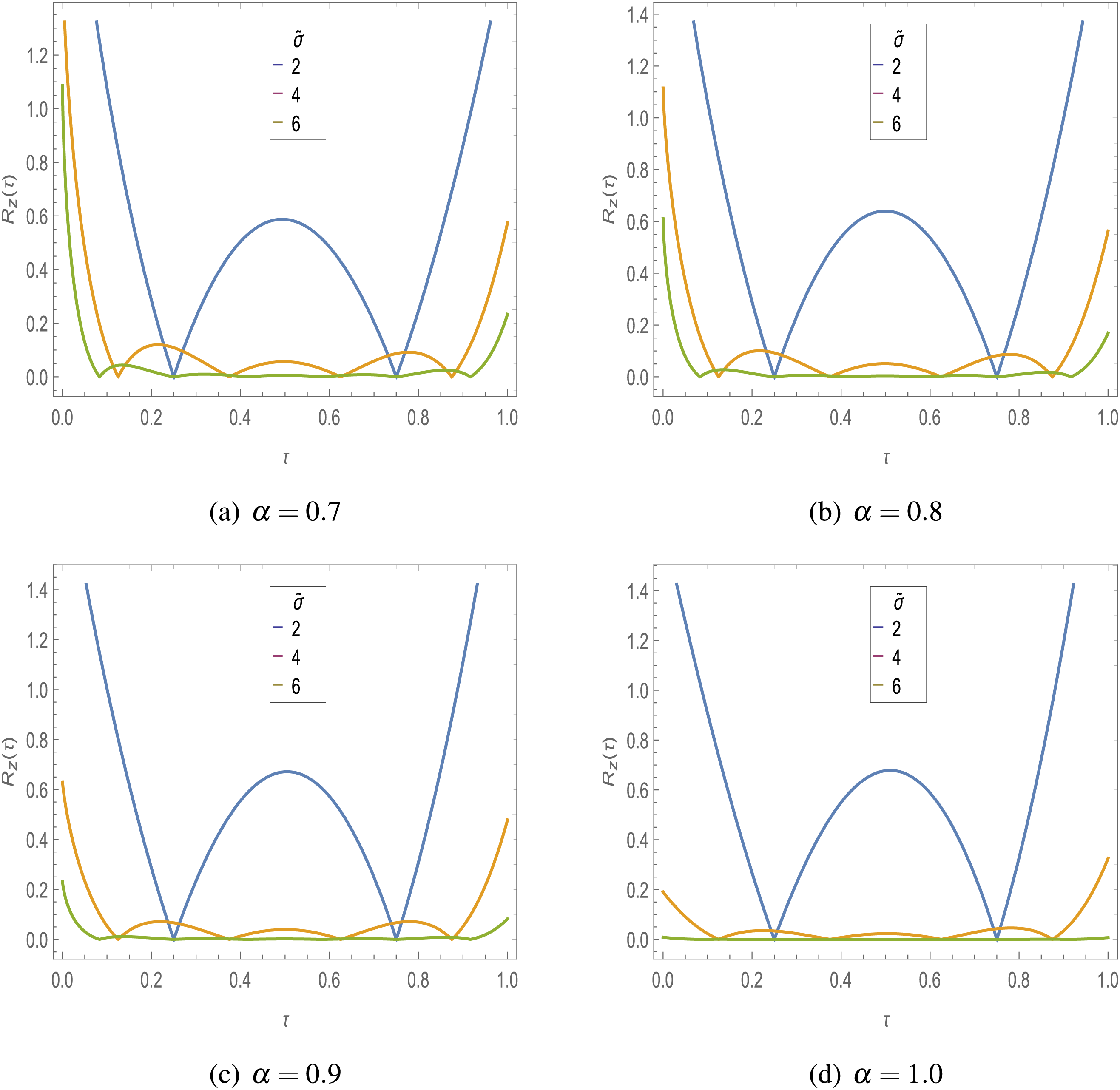
Figure 5: Residual error in
6.2 Symmetric Caputo Fractional Rössler Attractor Model
The symmetric Caputo fractional Rössler attractor model is numerically simulated for
For this case, the Rössler model is represented through the following equations as
with the conditions
Since there is no solution and no comparison available for integer and non-integer order of this model, therefore we simulated this model for different
At
At
At
At
The estimated residual errors in the solution of symmetric Caputo fractional Rössler attractor model for various values of
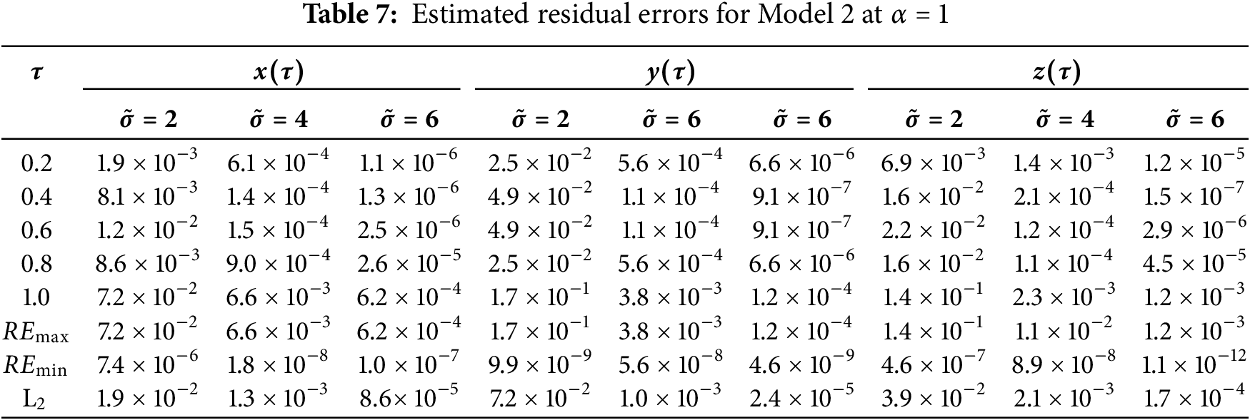

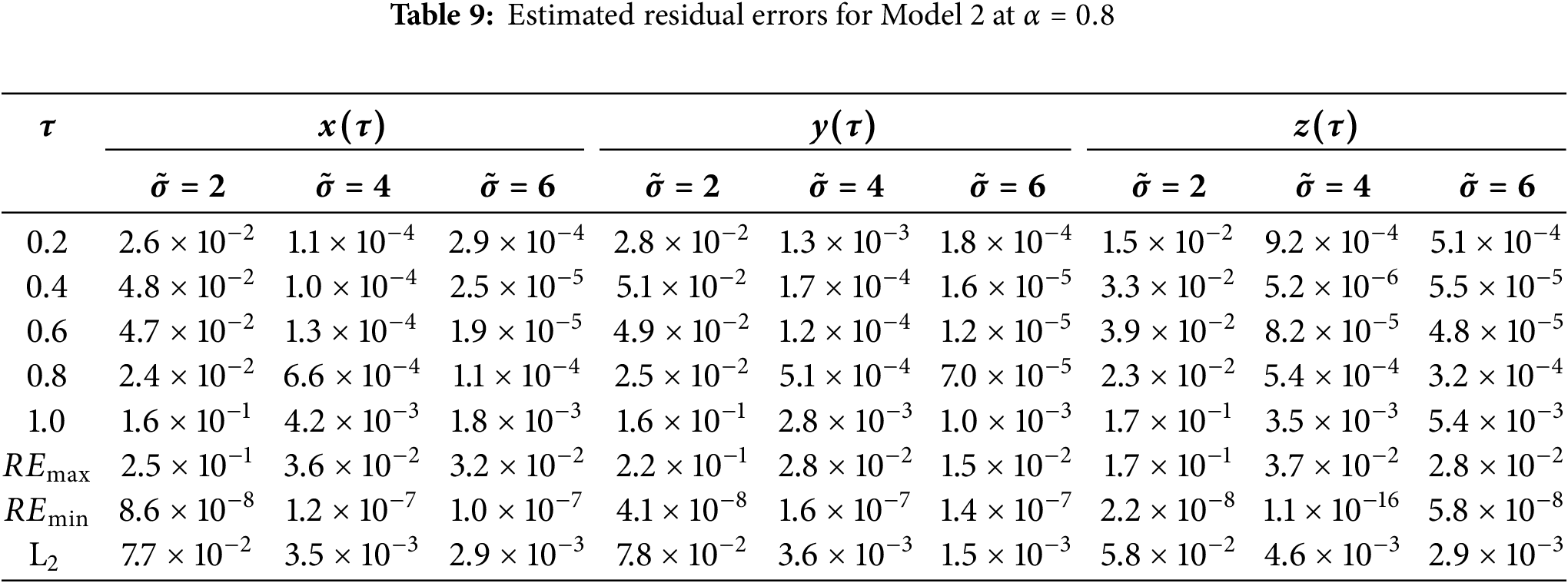
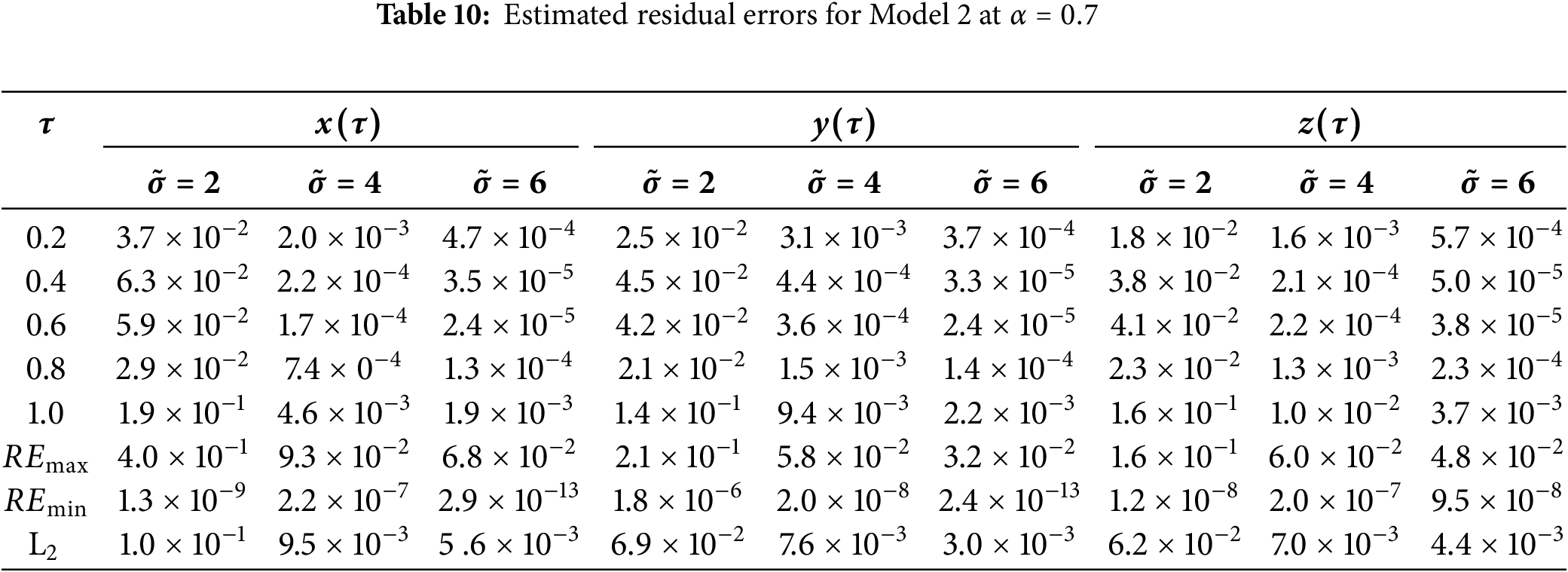

Figure 6: Solution of Model 2 via the suggested approach with fourth-order Range-Kutta method at
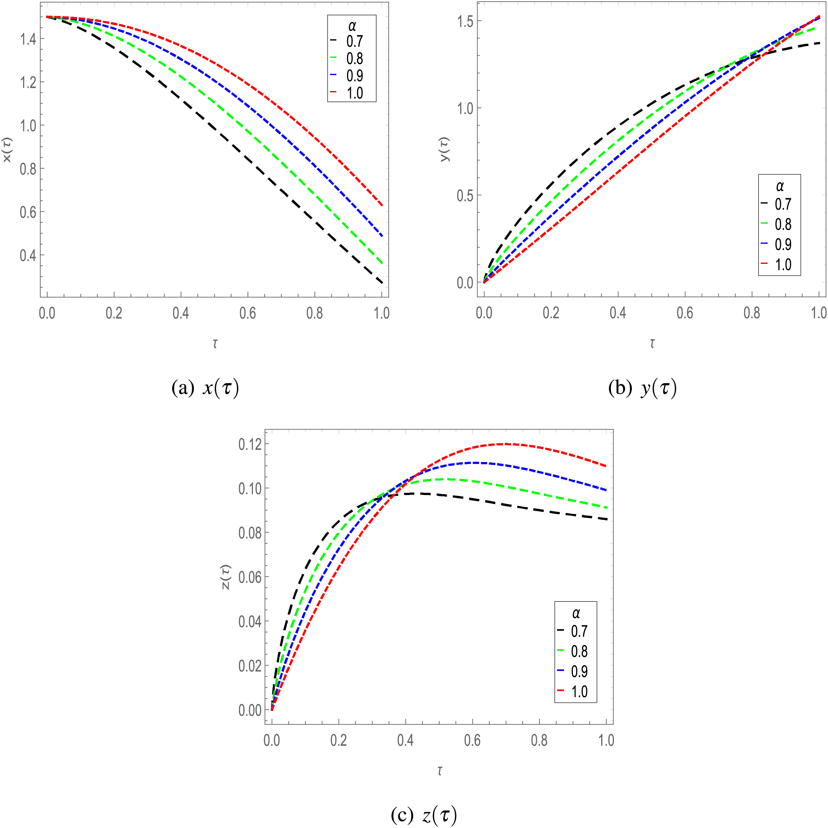
Figure 7: Solution of Model 2 for different

Figure 8: Residual error in
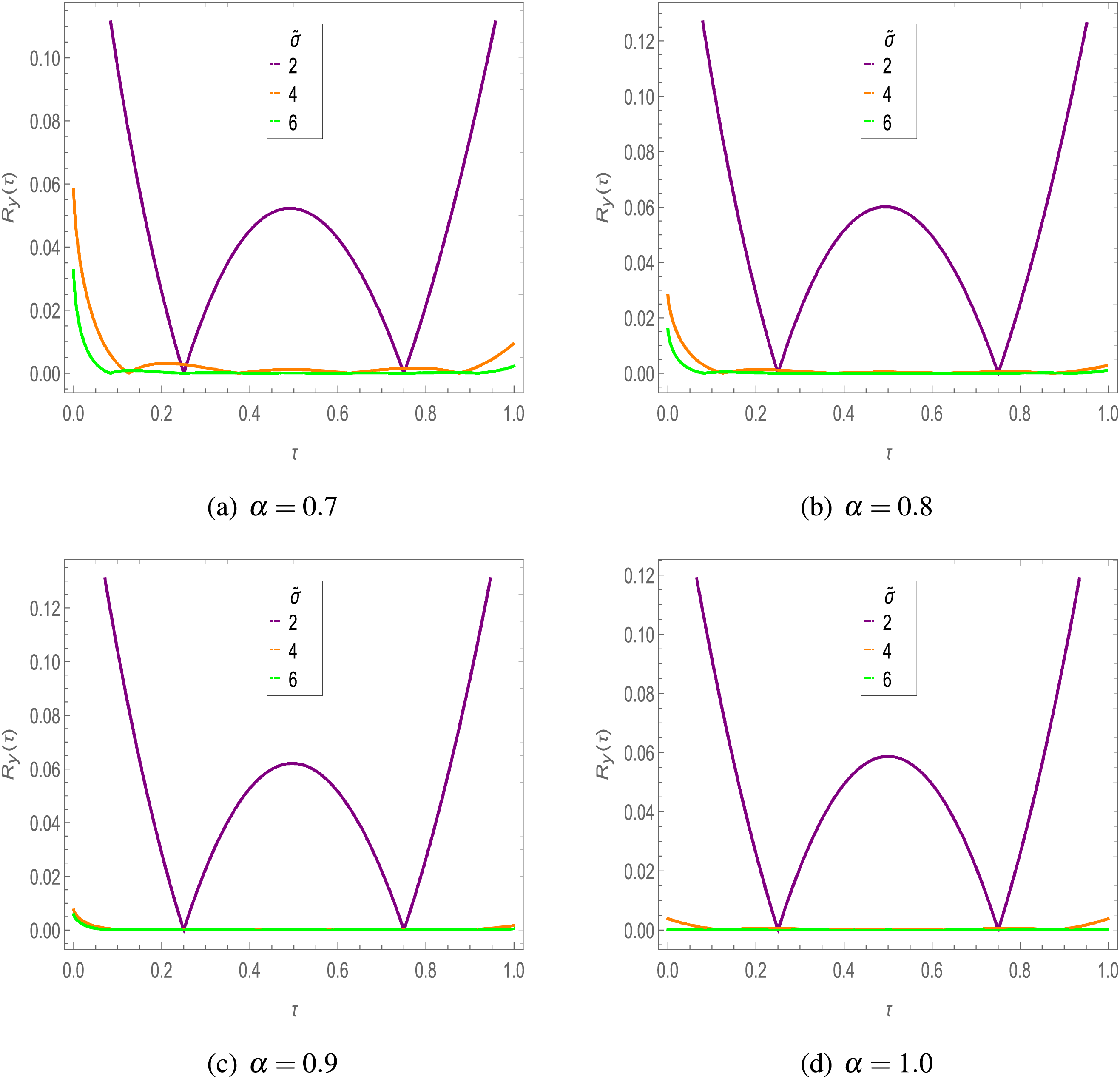
Figure 9: Residual error in
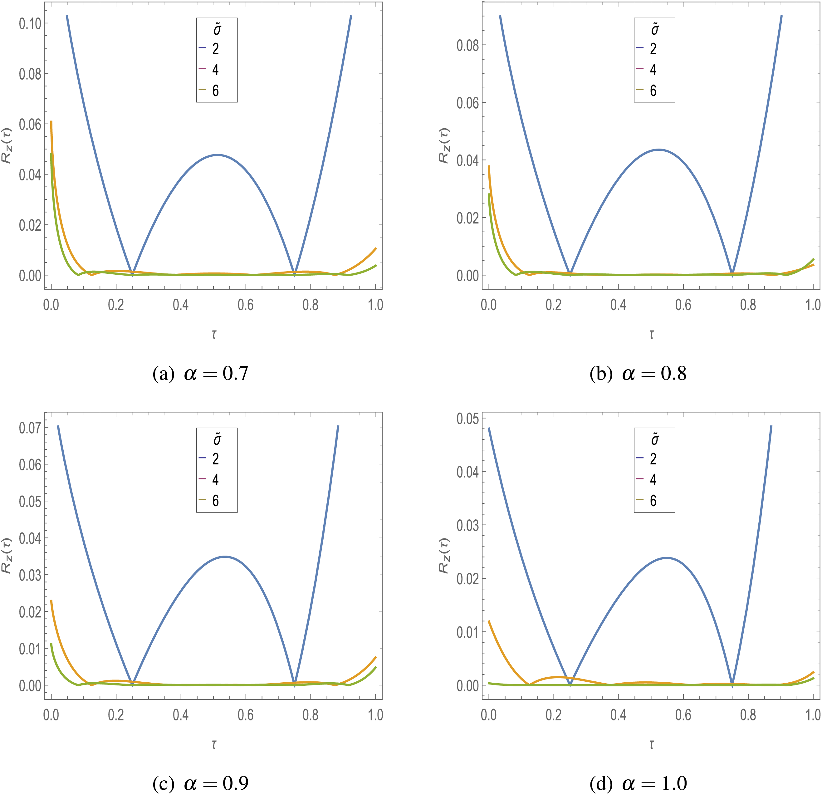
Figure 10: Residual error in
In this work, we investigated the dynamical behavior of the Caputo fractional Rössler attractor model using the Caputo differential operator, which inherits almost all features of the integer-order Rössler chaotic system in its dynamic properties. The Caputo fractional Rössler attractor model has been numerically investigated using the USWs approach which effectively and conveniently displays the solutions and residual errors. The success of the USWs-based approach in computing the accurate error for the Caputo fractional Rössler attractor model suggests that this approach has the potential to be employed in several other areas of engineering and technology. The exactness dependability of the Caputo fractional Rössler attractor model has been verified through
The study’s reliance on USWs offers computational advantages but may lead to high costs for large systems. Additionally, the scheme’s focus on a limited domain restricts broader applicability, and dynamic behaviors like bifurcations and stability remain underexplored, limiting the study’s generalizability.
Acknowledgement: None.
Funding Statement: “La derivada fraccional generalizada, nuevos resultados y aplicaciones a desigualdades integrales” Cod UIO-077-2024. This study is supported via funding from Prince Sattam bin Abdulaziz University project number (PSAU/2025/R/1446).
Author Contributions: Conceptualization, Ashish Rayal and Priya Dogra; Formal analysis, Ashish Rayal, Priya Dogra, Sabri T. M. Thabet, Imed Kedim and Miguel Vivas-Cortez; Funding acquisition, Miguel Vivas-Cortez; Investigation, Ashish Rayal, Priya Dogra, Sabri T. M. Thabet, Imed Kedim and Miguel Vivas-Cortez; Methodology, Ashish Rayal, Priya Dogra, Sabri T. M. Thabet, Imed Kedim and Miguel Vivas-Cortez; Software, Ashish Rayal and Priya Dogra; Validation, Ashish Rayal, Priya Dogra, Sabri T. M. Thabet and Imed Kedim; Writing—original draft, Ashish Rayal, Priya Dogra, Sabri T. M. Thabet, Imed Kedim and Miguel Vivas-Cortez; Writing—review & editing, Ashish Rayal, Priya Dogra, Sabri T. M. Thabet, Imed Kedim and Miguel Vivas-Cortez. All authors reviewed the results and approved the final version of the manuscript.
Availability of Data and Materials: All data generated or analyzed during this study are included in this published article.
Ethics Approval: Not applicable.
Conflicts of Interest: The authors declare no conflicts of interest to report regarding the present study.
References
1. Fleuren LM, Klausch TLT, Zwager CL, Schoonmade LJ, Guo T, Roggeveen LF, et al. Machine learning for the prediction of sepsis: a systematic review and meta-analysis of diagnostic test accuracy. Intensive Care Med. 2020;46(3):383–400. doi:10.1007/s00134-019-05872-y. [Google Scholar] [PubMed] [CrossRef]
2. Arefin S, Chowdhury M, Parvez R, Ahmed T, Abrar AFMS, Sumaiya F. Understanding APT detection using Machine learning algorithms: is superior accuracy a thing?. In: 2024 IEEE International Conference on Electro Information Technology (eIT); 2024; Eau Claire, WI, USA. p. 532–7. [Google Scholar]
3. Mora HM, Pont MT, Lopez FA, Pascual JM, Chamizo JM. Advancements in number representation for high-precision computing. J Super Comput. 2024;80(7):9742–61. doi:10.1007/s11227-023-05814-y. [Google Scholar] [CrossRef]
4. Madaliev M, Orzimatov J, Abdulkhaev Z, Esonov O, Mirzaraximov M. Several different ways to increase the accuracy of the numerical solution of the first order wave equation. BIO Web of Conf. 2024;84(2):02032. doi:10.1051/bioconf/20248402032. [Google Scholar] [CrossRef]
5. Debnath L. A brief historical introduction to fractional calculus. Int J Mathem Educat Sci Technol. 2004;35(4):487–501. doi:10.1080/00207390410001686571. [Google Scholar] [CrossRef]
6. Mani G, Gnanaprakasam AJ, Guran L, George R, Mitrovi’c ZD. Some results in fuzzy b-metric space with b-triangular property and applications to Fredholm integral equations and dynamic programming. Mathematics. 2023;11(19):4101. doi:10.3390/math11194101. [Google Scholar] [CrossRef]
7. Mani G, Gnanaprakasam AJ, Ege O, Aloqaily A, Mlaiki N. Fixed point results inC∗-algebra-valued partial b-metric spaces with related application. Mathematics. 2023;11(5):1158. doi:10.3390/math11051158. [Google Scholar] [CrossRef]
8. Mani G, Haque S, Gnanaprakasam AJ, Ege O, Mlaiki N. The study of bicomplex-valued controlled metric spaces with applications to fractional differential equations. Mathematics. 2023;11(12):2742. doi:10.3390/math11122742. [Google Scholar] [CrossRef]
9. Ross B. A brief history and exposition of the fundamental theory of fractional calculus. In: Ross B, editor. Fractional calculus and its applications. Lecture notes in mathematics. Berlin/Heidelberg: Springer; 1975. [Google Scholar]
10. Singh AP, Deb D, Agrawal H, Bingi K, Ozana S. Modeling and control of robotic manipulators: a fractional calculus point of view. Arab J Sci Eng. 2021;46(10):9541–52. doi:10.1007/s13369-020-05138-6. [Google Scholar] [CrossRef]
11. Wang H. Research on application of fractional calculus in signal real-time analysis and processing in stock financial market. Chaos, Solit Fract. 2019;128(1):92–7. doi:10.1016/j.chaos.2019.07.021. [Google Scholar] [CrossRef]
12. Wang Q, Ma J, Yu S, Tan L. Noise detection and image denoising based on fractional calculus. Chaos Solit Fract. 2020;131(4):109463. doi:10.1016/j.chaos.2019.109463. [Google Scholar] [CrossRef]
13. Baleanu D, Sajjadi SS, Jajarmi A, Defterli O. On a nonlinear dynamical system with both chaotic and nonchaotic behaviors: a new fractional analysis and control. Adv Differ Equ. 2021;234(1):148. doi:10.1186/s13662-021-03393-x. [Google Scholar] [CrossRef]
14. Ben-loghfyry A, Hakim A. Reaction-diffusion equation based on fractional-time anisotropic diffusion for textured images recovery. Int J Appl Comput Math. 2022;8(4):177. doi:10.1007/s40819-022-01380-8. [Google Scholar] [CrossRef]
15. Yang X, Gao F, Ju Y. General fractional derivatives with applications in viscoelasticity. Netherlands: Elsevier Science; 2020. [Google Scholar]
16. Tang TQ, Shah Z, Jan R, Alzahrani E. Modeling the dynamics of tumor-immune cells interactions via fractional calculus. Eur Phys J Plus. 2022;137(3):367. doi:10.1140/epjp/s13360-022-02591-0. [Google Scholar] [CrossRef]
17. Viera-Martin E, Gomez-Aguilar JF, Solis-Perez JE, Hernandez-Perez JA, Escobar-Jimenez RF. Artificial neural networks: a practical review of applications involving fractional calculus. Eur Phys J Spec Top. 2022;231(10):2059–95. doi:10.1140/epjs/s11734-022-00455-3. [Google Scholar] [PubMed] [CrossRef]
18. Harrouche N, Momani S, Hasan S, Al-Smadi M. Computational algorithm for solving drug pharmacokinetic model under uncertainty with nonsingular kernel type Caputo-Fabrizio fractional derivative. Alexandria Eng J. 2021;60(5):4347–62. doi:10.1016/j.aej.2021.03.016. [Google Scholar] [CrossRef]
19. Cristofaro L, Garra R, Scalas E, Spassiani I. A fractional approach to study the pure-temporal Epidemic Type Aftershock Sequence (ETAS) process for earthquakes modeling. Fract Calc Appl Anal. 2023;26(2):461–79. doi:10.1007/s13540-023-00144-5. [Google Scholar] [CrossRef]
20. Gorenflo R, Mainardi F. Fractional calculus: integral and differential equations of fractional order. Austria: Springer Vienna; 1997. [Google Scholar]
21. Odibat ZM, Al-Refai MA, Baleanu D. On some properties of generalized cardinal sine kernel fractional operators: advantages and applications of the extended operators. Chin J Phys. 2024;91: 349–60. [Google Scholar]
22. Shams M, Kausar N, Agarwal P, Jain S. Fuzzy fractional Caputo-type numerical scheme for solving fuzzy nonlinear equations. Fract Differ Equat, Acad Press. 2024;2(5):167–75. doi:10.1016/B978-0-44-315423-2.00016-3. [Google Scholar] [CrossRef]
23. Owolabi KM. Efficient numerical simulation of non-integer-order space-fractional reaction-diffusion equation via the Riemann-Liouville operator. The Eur Phys J Plus. 2018;133(3):1–16. doi:10.1140/epjp/i2018-11951-x. [Google Scholar] [CrossRef]
24. Jiang Y, Zhang B. Comparative study of Riemann-Liouville and Caputo derivative definitions in time-domain analysis of fractional-order capacitor. IEEE Transact Circ Syst II: Express Briefs. 2020;67(10):2184–8. doi:10.1109/TCSII.2019.2952693. [Google Scholar] [CrossRef]
25. Ghosh B, Mohapatra J. Analysis of finite difference schemes for Volterra integro-differential equations involving arbitrary order derivatives. J Appl Math Comput. 2023;69(2):1865–86. doi:10.1007/s12190-022-01817-9. [Google Scholar] [CrossRef]
26. Thabet STM, Dhakne MB. Nonlinear fractional integro-differential equations with two boundary conditions. Adv Studies Contemp Mathem. 2016;26(3):513–26. [Google Scholar]
27. Thabet STM, Dhakne MB. On boundary value problems of higher order abstract fractional integro-differential equations. Int J Nonl Anal Applicat. 2016;7(2):165–84. doi:10.22075/ijnaa.2017.520. [Google Scholar] [CrossRef]
28. Liu L, Chen S, Feng L, Zhu J, Zhang J, Zheng L, et al. A novel distributed order time fractional model for heat conduction, anomalous diffusion, and viscoelastic flow problems. Comput Fluids. 2023;265:105991. doi:10.1016/j.compfluid.2023.105991. [Google Scholar] [CrossRef]
29. Abdou MA. An analytical method for space-time fractional nonlinear differential equations arising in plasma physics. J Ocean Eng Sci. 2017;2(4):288–92. doi:10.1016/j.joes.2017.09.002. [Google Scholar] [CrossRef]
30. Alam M, Zada A, Abdeljawad T. Stability analysis of an implicit fractional integro-differential equation via integral boundary conditions. Alexandria Eng J. 2024;87(4):501–14. doi:10.1016/j.aej.2023.12.055. [Google Scholar] [CrossRef]
31. Thabet STM, Kedim I. Study of nonlocal multiorder implicit differential equation involving Hilfer fractional deriva-tive on unbounded domains. J Math. 2023;2023(3):1–14. doi:10.1155/2023/8668325. [Google Scholar] [CrossRef]
32. Rehman ZU, Boulaaras SM, Jan R, Ahmad I, Bahramand S. Computational analysis of financial system through non-integer derivative. J Comput Sci. 2023;75(12):102204. doi:10.1016/j.jocs.2023.102204. [Google Scholar] [CrossRef]
33. Dhobale SM, Chatterjee S. A general class of optimal nonlinear resonant controllers of fractional order with time-delay for active vibration control-theory and experiment. Mech Syst Signal Process. 2023;182(11):109580. doi:10.1016/j.ymssp.2022.109580. [Google Scholar] [CrossRef]
34. Rayal A, Negi P, Giri S, Baskonus HM. Taylor wavelet analysis and numerical simulation for boundary value problems of higher order under multiple boundary conditions. Pramana-J Phys. 2024;98(4):155. doi:10.1007/s12043-024-02825-z. [Google Scholar] [CrossRef]
35. Rayal A, Anand M, Srivastava VK. Application of fractional modified Taylor wavelets in the dynamical analysis of fractional electrical circuits under generalized Caputo fractional derivative. Phys Scr. 2024;99(12):125255. doi:10.1088/1402-4896/ad8701. [Google Scholar] [CrossRef]
36. Young RK. Wavelet theory and its applications. 1st ed. New York, NY, USA: Springer Science & Business Media; 2012. [Google Scholar]
37. Youssri YH, Abd-Elhameed WM, Doha EH. Ultraspherical wavelets method for solving Lane-Emden type equations. Rom J Phys. 2015;60(9–10):1298–314. [Google Scholar]
38. Farge M. Wavelet transforms and their applications to turbulence. Annual Rev Fluid Mech. 1992;24(1):395–458. doi:10.1146/annurev.fl.24.010192.002143. [Google Scholar] [CrossRef]
39. Rayal A, Verma SR. Numerical study of variational problems of moving or fixed boundary conditions by Muntz wavelets. J Vibrat Control. 2020;28:1–16. doi:10.1177/10775463209747. [Google Scholar] [CrossRef]
40. Rayal A, Patel PA, Giri S, Joshi P. A Comparative study of a class of Linear and Nonlinear Pantograph Differential Equations via different orthogonal polynomial Wavelets. Malaysian J Sci. 2024;43(2):75–95. doi:10.22452/mjs.vol43no2.9. [Google Scholar] [CrossRef]
41. Rayal A, Joshi P. A comprehensive review on fractional operators, wavelets, and their applications. Redshine Archive. 2024;11(4):380–7. [Google Scholar]
42. Rayal A, Bisht P, Giri S, Patel PA, Prajapati M. Dynamical analysis and numerical treatment of pond pollution model endowed with Caputo fractional derivative using effective wavelets technique. Int J Dyn Control. 2024;2024(12):1–14. doi:10.1007/s40435-024-01494-5. [Google Scholar] [CrossRef]
43. Rayal A, Verma SR. Two-dimensional Gegenbauer wavelets for the numerical solution of tempered fractional model of the nonlinear Klein-Gordon equation. Appl Numer Math. 2022;174(10):191–220. doi:10.1016/j.apnum.2022.01.015. [Google Scholar] [CrossRef]
44. Rayal A, Anand M, Chauhan K, Prinsa. An overview of mamadu-njoseh wavelets and its properties for numerical computations. Uttaranchal J Appl Life Sci. 2023;4(1):1–8. [Google Scholar]
45. Rayal A. An effective Taylor wavelets basis for the evaluation of numerical differentiations. Palestine J Mathem. 2023;12:551–68. [Google Scholar]
46. Rayal A. Muntz wavelets solution for the polytropic lane-emden differential equation involved with conformable type fractional derivative. Int J Appl Comput Math. 2023;9(4):50. doi:10.1007/s40819-023-01528-0. [Google Scholar] [CrossRef]
47. Rayal A, Joshi BP, Pandey M, Torres DFM. Numerical investigation of the fractional oscillation equations under the context of variable order caputo fractional derivative via fractional order bernstein wavelets. Mathematics. 2023;11(11):2503. doi:10.3390/math11112503. [Google Scholar] [CrossRef]
48. Rayal A, Verma SR. Numerical analysis of pantograph differential equation of the stretched type associated with fractal-fractional derivatives via fractional order Legendre wavelets. Chaos Solit Fract. 2020;139(1):110076. doi:10.1016/j.chaos.2020.110076. [Google Scholar] [CrossRef]
49. Devaney RL. An introduction to chaotic dynamical systems. Boca Raton, FL, USA: CRC Press; 2021. [Google Scholar]
50. Atangana A, Qureshi S. Modeling attractors of chaotic dynamical systems with fractal-fractional operators. Chaos Solit Fract. 2019;123(3):320–37. doi:10.1016/j.chaos.2019.04.020. [Google Scholar] [CrossRef]
51. Shen BW, Pielke SRRA, Zeng X, Baik JJ, Faghih-Naini S, Cui J, et al. Is weather chaotic? Coexisting chaotic and non-chaotic attractors within Lorenz models. Vol. 13. In: 13th Chaotic Modeling and Simulation International Conference. Springer Proceedings in Complexity. Cham: Springer; 2021. p. 805–25. [Google Scholar]
52. Desharnais RA, Henson SM, Costantino RF, Dennis B. Capturing chaos: a multidisciplinary approach to nonlinear population dynamics. J Differ Equat Applicat. 2023;30(8):1002–39. doi:10.1080/10236198.2023.2260013. [Google Scholar] [CrossRef]
53. Lahmiri S. Assessing efficiency in prices and trading volumes of cryptocurrencies before and during the COVID-19 pandemic with fractal, chaos, and randomness: evidence from a large dataset. Financ Innovation. 2024;10(1):82. doi:10.1186/s40854-024-00628-0. [Google Scholar] [CrossRef]
54. Zhang B, Liu L. Chaos-based image encryption: review, application, and challenges. Mathematics. 2023;11(11):2585. doi:10.3390/math11112585. [Google Scholar] [CrossRef]
55. Shen BW. A review of lorenz’s models from 1960 to 2008. Int J Bifurcat Chaos. 2023;33(10):2330024. doi:10.1142/S0218127423300240. [Google Scholar] [CrossRef]
56. Corona-Bermudez E, Chimal-Eguia JC, Corona-Bermudez U, Rivero-Angeles ME. Chaos meets cryptography: developing an S-box design with the rössler attractor. Mathematics. 2023;11(22):4575. doi:10.3390/math11224575. [Google Scholar] [CrossRef]
57. Rössler OE. An equation for continuous chaos. Phys Letters A. 1976;57:397–8. [Google Scholar]
58. Li C, Hu W, Sprott JC, Wang X. Multistability in symmetric chaotic systems. Eur Phys J Spec Top. 2015;224(8):1493–506. doi:10.1140/epjst/e2015-02475-x. [Google Scholar] [CrossRef]
59. Kontorovich VY, Beltran LA, Aguilar JM, Lovtchikova Z, Tinsley KR. Cumulant analysis of Rössler attractor and its applications. The Open Cybernet Syst J. 2009;3:29–39. [Google Scholar]
60. Rysak A, Sedlmayr M, Gregorczyk M. Revealing fractionality in the Rössler system by recurrence quantification analysis. The Eur Phy J Spec Topics. 2023;232(1):83–98. doi:10.1140/epjs/s11734-022-00740-1. [Google Scholar] [CrossRef]
61. Elbadri M, Abdoon MA, Berir M, Almutairi DK. A numerical solution and comparative study of the symmetric rossler attractor with the generalized caputo fractional derivative via two different methods. Mathematics. 2023;11(13):2997. doi:10.3390/math11132997. [Google Scholar] [CrossRef]
62. Kekana MC, Shatalov MY, Tong TO, Fadugba SE. Analysis of Rossler attractor by means of residual and Joubert-Greeff methods. South East Asian J Mathem Mathem Sci. 2023;19(02):431–50. doi:10.56827/SEAJMMS.2023.1902.32. [Google Scholar] [CrossRef]
63. Barrio R, Blesa F, Serrano S. Qualitative analysis of the Rössler equations: bifurcations of limit cycles and chaotic attractors. Physica D: Nonlin Phenom. 2009;238(13):1087–100. doi:10.1016/j.physd.2009.03.010. [Google Scholar] [CrossRef]
64. Santra MS, Gaur SS, Gupta A. Numerical solution of Rössler attractor using power series method. Int Res J Adv Eng Manag. 2024;2(3):182–6. doi:10.47392/IRJAEM.2024.0028. [Google Scholar] [CrossRef]
65. Boulehmi K. A novel numerical scheme for fractional bernoulli equations and the Rössler model: a comparative analysis using atangana-baleanu caputo fractional derivative. Eur J Pure Appl Mathem. 2024;17(1):445–61. doi:10.29020/nybg.ejpam.v17i1.5043. [Google Scholar] [CrossRef]
66. Odibat ZM, Baleanu D. Numerical simulation of initial value problems with generalized Caputo-type fractional derivatives. Appl Num Mathem. 2020;156(6):94–105. doi:10.1016/j.apnum.2020.04.015. [Google Scholar] [CrossRef]
67. Askey R, Ismail MEH. A generalization of ultraspherical polynomials. Birkhäuser Basel, Switzerland, 1983. [Google Scholar]
68. Abd-Elhameed WM, Youssri YH. New spectral solutions of multi-term fractional-order initial value problems with error analysis. Comput Model Eng Sci. 2015;105(5):375–98. doi:10.3970/cmes.2015.105.375. [Google Scholar] [CrossRef]
69. Ozdemir N, Secer A. A numerical algorithm based on ultraspherical wavelets for solution of linear and nonlinear Klein Gordon equations. Sigma J Eng Natural Sci. 2020;38(3):1307–19. [Google Scholar]
70. Artin E. The gamma function. Garden City, NY, USA: Dover Publications; 2015. [Google Scholar]
71. Tavazoei MS, Haeri M. Chaotic attractors in incommensurate fractional order systems. Physica D. 2008;237(20):2628–37. doi:10.1016/j.physd.2008.03.037. [Google Scholar] [CrossRef]
72. Mehdi SA, Kareem RS. Using fourth-order Runge-kutta method to solve lu chaotic system. Am J Eng Res. 2017;6(1):72–7. [Google Scholar]
Cite This Article
 Copyright © 2025 The Author(s). Published by Tech Science Press.
This work is licensed under a Creative Commons Attribution 4.0 International License , which permits unrestricted use, distribution, and reproduction in any medium, provided the original work is properly cited.
 Downloads
 Citation Tools