Shock-Capturing Particle Hydrodynamics with Reproducing Kernels

1  Introduction

The Smoothed Particle Hydrodynamics (SPH) method was originally developed to solve astrophysical gas dynamics problems [1,2]. In an SPH simulation, the particle distribution automatically adapts to the dynamics of the gas flow, and this has major advantages when, for example, modeling the gravitational collapse of gas clouds that condense into denser filaments and finally form stars. The natural geometric adaptivity of SPH also has advantages in many other contexts where challenging geometries are involved, e.g., in simulating dam breaks, e.g., [3], or fracture processes, e.g., [4], see [5] for a broad range of SPH applications. Since the particles automatically follow the gas flow, this also implies that vacuum is simply modeled by the absence of computational particles. Eulerian methods, in contrast, need to model vacuum as a low-density background gas, and this can cost substantial computational resources even though one is not interested (and nothing is physically going on) in empty space. As an admittedly extreme, but astrophysically relevant example, we show in Fig. 1 the tidal disruption of two stars by a massive black hole located at the coordinate origin (the simulation is discussed in more detail in [6]). As the stars pass the black hole, they are ripped apart by the hole’s tidal forces. One is only interested in the fate of the gas from the disrupted stars, which initially covers only a minute fraction of 10−9 of the space shown in Fig. 1. So, in a corresponding Eulerian simulation, one would need to waste essentially all of the computational resources to simulate the uninteresting empty space. Another major advantage of SPH is that it can be formulated in a way that Nature’s conservation laws are enforced by construction [7–11]. Having Nature’s conservation laws built into a simulation gives some confidence that the simulated system behaves similarly to what Nature does.

Figure 1: Illustration of one of SPH’s most salient features: the natural treatment of vacuum. The plot shows how two stars have been ripped apart by a black hole (lurking at the coordinate origin) into spaghetti-like, thin gas streams that are held together by the gas’ self-gravity. The inset shows the initial conditions of the initially spherical stars. The original stars in the inset only cover a fraction of 10−9 of the volume that is shown at late times (t = 371 h). Simulation performed with the MAGMA2 code, see Rosswog (2020)

Simulating gas flows with particles is still a relatively young field compared to Eulerian gas dynamics, and much development is still ongoing, both in terms of methodology and in terms of spreading into new research areas. For example, most recently, SPH methods have found their way into general relativistic hydrodynamics where the full spacetime is dynamically evolved together with the fluid, see [12,13], or Chap. 7 in [14]. SPH has initially been criticized for many issues, but essentially all of them have seen major improvements achieved in recent times. For example, SPH has often been criticized for being too dissipative. However, as derived from a Lagrangian, SPH contains zero dissipation, and the criticism goes back to the early days of SPH when simple artificial dissipation schemes were used, in which dissipation was always switched on, whether needed or not. In recent years, much effort has been spent to cure this problem, e.g., by using time-dependent dissipation parameters that only reach substantial values when needed, but not otherwise [15–19] or by using slope-limited reconstruction in the artificial dissipation terms [20,21,12,13,22]. The latter approach is very effective even if large constant dissipation parameters are used. For example, some weakly triggered Kelvin-Helmholtz instabilities do not grow when standard, constant dissipation parameters without reconstruction are used, but the same initial conditions lead to a healthy growth of instability when reconstruction is applied; see Fig. 20 in [21].

As an alternative to artificial dissipation, one can also implement Riemann solvers into SPH [23–27] to produce sufficient entropy in shocks. However, with this approach, one also needs to ensure that not too much unwanted dissipation is introduced. For example, simply treating particle pairs as Riemann problems, where the left and the right states are given by the particle properties, leads to very dissipative hydrodynamics unless other measures such as limiters or reconstruction techniques similar to Finite Volume schemes are applied. Often, Riemann solver approaches are only benchmarked against shocks, where they perform, by construction, very well. However, such approaches can still be way too dissipative to accurately model the growth of weakly triggered fluid instabilities.

It has also turned out that the still frequently used cubic spline kernel is not a great choice after all, but substantially better kernels are readily available [18,28–30] and replacing the kernel function only requires very small changes to existing codes. It has further been realized that much more accurate gradient estimates [18,31,32] than the standard kernel gradients can be obtained at a moderate additional cost and even without sacrificing the highly valued kernel anti-symmetry, ∇aWab=−∇bWab, which is crucial for good numerical conservation, see e.g., Section 2.4 in [8].

Several of the above improvements of SPH have borrowed techniques that are traditionally used in Finite Volume schemes, such as reconstruction, slope-limiting, or Riemann solvers. For example, recent work has explored the application of weighted essentially non-oscillatory (WENO) strategies to SPH; see e.g., [33–36]. Apart from “enhanced SPH”, there is also a class of methods that tries to consistently formulate the ideal gas dynamics equations from the beginning as in Finite Volume methods, though for particles rather than for meshes, see e.g., [37–41] for some pioneering work. This also comes with a broad variety of names for relatively similar methods, some of which are “proper SPH”, some are “SPH with elements from Finite Volume methods”, and yet others are proper Finite Volume discretizations of the conservation laws written for particles. Among these latter methods, there are formulations for stationary particles (Eulerian), for particles that move with the fluid velocity (Lagrangian) or for particles that move with any other velocity (Adaptive Lagrangian Eulerian or ALE methods); see, e.g., [42]. Therefore, the boundaries between different methods are blurred, and it becomes a matter of semantics or taste how to call a given method. In summary, many of the issues that SPH has been criticized for can be considered as essentially solved, and modern SPH formulations can accurately solve very challenging gas dynamics problems1, for example [20–22].

One issue that has been strongly improved by the above measures but is usually still not exactly enforced in the standard SPH approaches is the lack of zero-order consistency. In simple words, the SPH approximation makes use of weighted kernel sums over neighboring particles, but the weights in these sums do not add up exactly to unity; see our discussion in Section 2.4. Whether this is an issue in practical applications or not depends on the kernels/neighbor numbers that are used and the tested problem considered, but it is desirable to avoid the issue in the first place. Without zeroth-order consistency, not even constant functions are reproduced exactly.

In this paper, we formulate and explore a new approach, in which we start from one of the commonly used SPH discretizations, but a) we introduce Roe’s approximate solver, b) we identify the dissipative terms in the Riemann solver, and in these terms, we use slope-limited reconstruction, and finally, c) we use linearly reproducing kernels so that constant and linear functions are reproduced to machine precision. We carefully scrutinize our implementation of the reproducing kernels and put the new method to the test with many very challenging benchmark tests, ranging from shocks over fluid instabilities to vorticity creating Schulz-Rinne shocks [43]. All of these tests are performed in three spatial dimensions. In Section 2, we discuss all the elements involved in our approach, and in Section 3, we present and discuss our benchmark tests before we summarize and conclude in Section 4.

2  Methodology

2.1 Particle Hydrodynamics Formulation with a Riemann Solver

In the following, we will label the particles with a,b and k, where a is usually the particle of interest, b a neighbor particle, and k can be either of them. We also use the Einstein sum convention with repeated indices, which implies a sum from 1 to 3, and we usually use i,j,l and m for the summation indices. Since we are working in a non-relativistic context and do not have to distinguish between co- and contravariant vectors, it has no particular meaning whether an index is written as a subscript or a superscript; readability considerations mostly guide this.

Our starting point is a common set of Smoothed Particle Hydrodynamics (SPH) equations [24,44,27]

ρa=∑bmbW¯ab(1)

dv→adt=−∑bmbPa+Pbρaρb∇aW¯ab(2)

duadt=12∑bmbPa+Pbρaρbv→ab⋅∇aW¯ab.(3)

In Eqs. (2) and (3), the index a at the nabla operator indicates that it is evaluated with respect to particle a (and not b). As usual, one has the choice between either solving the continuity equation directly or obtaining the density ρa through a kernel-weighted sum over neighbors, see Eq. (1), which is our choice here. The continuity equation approach has been found to be advantageous in some recent studies [22,27], but we choose here the summation approach, since it is guaranteed to deliver a strictly positive density due to the positive definite kernels W that we are using. Alternatives to this approach will be explored in the future. The size of the kernel support is determined by the smoothing length h, P denotes the gas pressure, u is the specific internal energy, and v→ab=v→a−v→b. Often, the density estimation, Eq. (1), is performed “as locally as possible” in the sense that the kernel of a particle a is evaluated with its smoothing length, ha. To be consistent with our later choices, see Section 2.4, we choose here

W¯ab=W(|r→a−r→b|/ha)+W(|r→a−r→b|/hb)2and∇W¯ab=∇W(|r→a−r→b|/ha)+∇W(|r→a−r→b|/hb)2.(4)

While we have written the above equations in a commonly used way, it is worth keeping in mind that the kernel gradient can be explicitly written (for some smoothing length h) as

∇aWab(h)=∂W(qab)∂qab∂qab∂r→a=∂W(qab)∂qabe^abh,(5)

where qab=|r→a−r→b|/h and e^ab=(r→a−r→b)/|r→a−r→b| is the unit vector pointing from particle b to particle a. With this, Eq.(3) can also be written as

duadt=12∑bmbPa+Pbρaρb(v→a⋅e^ab−v→b⋅e^ab)1hab∂W∂qab=12∑bmbPa+Pbhab ρaρb∂W∂qab(v~a−v~b),(6)

where the velocities projected on the connection line are marked with a tilde.

In gas dynamics, seemingly harmless sound waves can steepen into shock waves, and for their correct treatment, dissipation is needed. So far, however, the equations are entirely nondissipative, and to handle shocks, they need to be enhanced by mechanisms that produce sufficient (but not too much) dissipation to obtain non-oscillatory solutions in shocks. As outlined in the introduction, an often used approach is artificial viscosity, which has seen many improvements in recent times, including more accurate ways to steer dissipation parameters [17–19], applying reconstruction techniques in dissipative terms [20–22]. These new developments have also been transferred to (general) relativistic hydrodynamics [12,13,45]. These new approaches have turned out to be robust and accurate and to produce very little unwanted dissipation. In our understanding, such modern artificial dissipation approaches are on par with approximate Riemann solvers.

Despite the very good performance of modern artificial viscosity schemes, we want to explore here the case where dissipation is provided by a Riemann solver [46]. The main idea is to solve (approximately) a one-dimensional Riemann problem at the midpoint between each pair of interacting particles a and b, as sketched in Fig. 2. More specifically, we replace averages of particle values by the solution of a Riemann problem

Pa+Pb2→Pab∗andv~a+v~b2→vab∗,(7)

where the ∗ labels the contact discontinuity state in a Riemann problem, see e.g., [46], and the ab-index refers to the solution between state a and b. As before, the tilde denotes the velocities projected onto the line connecting two particles

v~a=v→a⋅e^abandv~b=v→b⋅e^ab.(8)

Figure 2: To add dissipation, Riemann problems are solved for each particle and its neighbour particles

With the substitutions Eq. (7) we have

Pa+Pb=2Pab∗andv~a−v~b=2(v~a−vab∗)(9)

so that the hydrodynamics equations, now with dissipation, read

ρa=∑bmbW¯ab,(10)

dv→adt=−2ρa∑bVbPab∗∇aW¯ab,(11)

duadt=2ρa∑bVbPab∗(v→a−v→ab∗)⋅∇aW¯ab,(12)

where we have used Vb=mb/ρb and v→ab∗=vab∗e^ab.

2.2 Dissipation in the Roe Solver

We use Roe’s approximate Riemann solver [47] for the star state:

vab∗=12((v→a+v→b)⋅e^ab+Pb−PaCRL),(13)

Pab∗=12(Pa+Pb+CRL(v→b−v→a)⋅e^abCRL),(14)

where the “densitized” Roe-averaged Lagrangian sound speed (the dimension is density times velocity) is

CRL=cs,aρaρa+cs,bρbρbρa+ρb,(15)

and cs,k is the sound speed of particle k. If, for a moment, we ignore the terms that involve the pressure and velocity differences in Eqs. (13) and (14), we have

vab∗≈v→a+v→b2⋅e^abandPab∗≈Pa+Pb2.(16)

By inserting these expressions into Eqs. (11) and (12) we obviously recover the inviscid Eqs. (2) and (3), therefore the terms involving the differences in Eqs. (13) and (14) are responsible for the dissipation. One may thus try to cure potentially excessive dissipation by modifying these terms. We approach this issue here by applying the reconstructed pressure and velocity values in the dissipative terms. So, for perfectly reconstructed smooth flows, where the reconstructed values on both sides of the midpoint are the same and, therefore, the dissipative terms vanish, one effectively solves the inviscid hydrodynamics equations.

2.3 Reconstruction in the Dissipative Terms

Our strategy to reduce dissipation is to use, in the dissipative terms of Eqs. (13) and (14), values of P and v→ that are reconstructed to the midpoint of each particle pair, r→abmid=0.5(r→a+r→b), see Fig. 2, left panel. So, at each interparticle midpoint, one has P/v→ values that are reconstructed once from the a-side and once from the b-side. Explicitly, the linearly reconstructed velocity components read

vai,rec=vai−12Ψ(∇vai,∇vbi)⋅r→ab,(17)

vbi,rec=vbi+12Ψ(∇vai,∇vbi)⋅r→ab,(18)

the specific internal energy is

uarec=ua−12Ψ(∇ua,∇ub)⋅r→ab,(19)

ubrec=ub+12Ψ(∇ua,∇ub)⋅r→ab,(20)

and the density

ρarec=ρa−12Ψ(∇ρa,∇ρb)⋅r→ab,(21)

ρbrec=ρb+12Ψ(∇ρa,∇ρb)⋅r→ab.(22)

With the reconstructed values of internal energy and density, we can calculate the corresponding pressure values via our equation of state, P=(γ−1)ρu.

The quantity Ψ in the above reconstruction equations is a suitable slope limiter function. Commonly used slope limiters are minmod

Ψmm(x,y)=12[SGN(x)+SGN(y)] MIN(|x|,|y|),(23)

the vanLeer limiter [48]

ΨvL(x,y)={2xyx+yif xy>00otherwise,(24)

the vanLeer monotonized Central (vanLeerMC) [48]

ΨvLMC(x,y)={SGN(x) MIN[|x+y|2,2|x|,2|y|]if xy>00otherwise,(25)

and the vanAlbada limiter [49]

ΨvA(x,y)={(x2+ϵ2)y+(y2+ϵ2)xx2+y2+2ϵ2if xy>0,0otherwise.(26)

The latter is insensitive to the exact value of ϵ, here, we use ϵ2=10−6. In Eqs. (19) to (22), the slope limiter Ψ is to be applied to each component of the gradients.

2.4 Linearly Reproducing Kernel (RPK) Approximations

One of the main criticisms of the standard SPH method is that it, in general, does not exactly reproduce constant or linear functions. In the standard SPH-discretization the approximation of a function f(r→) reads

f~(r→)=∑b Vb fb W(r→−r→b,h(r→))=∑bfb Φb(r→),(27)

where we have abbreviated mb/ρb as Vb and the smoothing length h should be thought of as a function of r→. After the second equal sign, we have abbreviated the product VbW(r→−r→b,h(r→)) as weight function Φb(r→). As an example, if all function values would be the same, fb=f0, then the function approximation should yield f0, but the standard SPH approximation finds

f~(r→)=f0∑bmbρbW(r→−r→b,h)≈f0,(28)

which is approximately, but not exactly, equal to the desired value, because the sum is not guaranteed to yield exactly unity. More systematically, one can expand fb (i.e., the function f at the position b) around r→, insert this into Eq. (27) to find

f~(r→)=∑b[f(r→)+(∇f)(r→)⋅(rb→−r→)+h.o.t.] Φb(r→)=f(r→)∑bΦb(r→)+(∇f)(r→)⋅∑b(rb→−r→)Φb(r→)+h.o.t.,(29)

where higher order terms are abbreviated as “h.o.t”. This implies, not too surprisingly, that for a good approximation, f~(r→)≈f(r→), the lowest order consistency relations

∑bΦb(r→)=1and∑b(r→b−r→)i Φb(r→)=0,(30)

should be fulfilled. Standard SPH usually fulfils this well in initial conditions (where particles are often placed on some type of lattice), but it does not enforce these conditions during evolution. The conditions are well fulfilled when good kernels (e.g., of the Wendland family [28]) with large neighbour numbers are used [18], but this, of course, comes at the price of expensive sums over many neighboring particles.

The consistency relations Eq. (30), however, can also be enforced by construction, e.g., in the so-called reproducing kernel method [50]. One can, for example, enhance the kernel functions with additional parameters A and Bi,

𝒲ab(r→ab)=Aa[1+Bai (r→ab)i]W¯ab,(31)

where W¯ab is given by Eq. (4). One can then determine the four unknown numbers A and Bi by enforcing the four discrete consistency relations so that

∑bVb 𝒲ab=1and∑bVb (r→ab)i 𝒲ab=0,(32)

is fulfilled at every particle position r→a. Since these kernels 𝒲ab reproduce by construction constant and linear functions exactly (i.e., to floating point accuracy), they are usually referred to as (linearly) reproducing kernels (RPKs). Reconstructing kernels for higher-order polynomials could be designed similarly, but at the price of lengthy and computationally expensive-to-evaluate expressions. We, therefore, restrict ourselves here to linear order. Since the Bi are in general non-zero, the kernels 𝒲ab are not guaranteed to be radial as standard SPH kernels, and therefore, angular momentum conservation is difficult to enforce exactly. In SPH, angular momentum conservation is usually a consequence of the interparticle forces pointing along the connecting vectors between a particle a and a particle b, e^ab, together with the kernel being anti-symmetric, ∇aWab=−∇bWab, see Section 2.4 in [8] for a detailed discussion. It is, however, still possible to write a set of equations that conserves energy and momentum (and mass if density summation is used), but not necessarily angular momentum. In practice, however, this does not seem to be a major concern; for example, the authors of [20] find with their artificial viscosity-based RPK-SPH approach in typical tests violations of exact angular momentum conservation on the sub-percent level.

The gradient of 𝒲ab can be calculated in a straight-forward way as

(∇a)k𝒲ab=Aa Bak W¯ab+Aa(1+Bai(r→ab)i)∇akW¯ab+(1+Bai(r→ab)i)W¯ab(∂kA)a+Aa (r→ab)i (∂kB)ai W¯ab.(33)

Now, taking the nabla operator concerning particle b, one finds

(∇b)k𝒲ba=Ab Bbk W¯ba+Ab(1+Bbi(r→ba)i)∇bkW¯ba+(1+Bbi(r→ba)i)W¯ba(∂kA)b+Ab (r→ba)i (∂kB)bi W¯ba=Ab Bbk W¯ab+Ab(1+Bbi(r→ab)i)∇akW¯ab+(1−Bbi(r→ab)i)W¯ab(∂kA)b−Ab (r→ab)i (∂kB)bi W¯ab,(34)

where we have used W¯ab=W¯ba, r→ba=−r→ab and ∇bkW¯ba=−∇akW¯ab. The parameters A and Bi and their derivatives, which are needed for ∂k𝒲ab, can then be calculated by straightforward algebra. We first define discrete moments at position r→a as

(M0)a≡∑bVb W¯ab,(35)

(M1i)a≡∑bVb (r→ab)iW¯ab,(36)

(M2ij)a≡∑bVb (r→ab)i (r→ab)j W¯ab.(37)

and their derivatives read

(∂kM0)a≡∑bVb ∇akW¯ab,(38)

(∂kM1i)a≡∑bVb[(r→ab)i(∇akW¯ab)+δkiW¯ab],(39)

(∂kM2ij)a≡∑bVb [(r→ab)i (r→ab)j (∇akW¯ab)+(r→ab)i δjk W¯ab+(r→ab)j δik W¯ab].(40)

With the moments and their derivatives at hand, one can calculate the kernel parameters

Aa=1(M0)a−(M2ij)a−1 (M1i)a (M1j)a,(41)

Bai=−(M2ij)a−1 (M1j)a,(42)

and their somewhat lengthy but otherwise straightforward calculable derivatives

∂kAa=−Aa2[(∂kM0)a−2(M2ij)a−1(M1j)a(∂kM1i)a+(M2il)a−1(∂kM2lm)a(M2mj)a−1(M1j)a(M1i)a],(43)

and

∂kBai=−(M2ij)a−1 (∂kM1j)a+(M2il)a−1 (∂kM2lm)a(M2mj)a−1(M1j)a.(44)

With the linearly reproducing kernels now at hand, we can approximate a function F via

F~(r→a)=∑bVb Fb 𝒲ab,(45)

and its derivative via

∂kF~(r→a)=∑bVb Fb ∂k𝒲ab.(46)

While these expressions look very similar to standard SPH approximations, they exactly reproduce linear functions on a discrete level, which the SPH equations do not.

Scrutinizing Our Implementation

To test our implementation of the linear reproducing kernels, we start from a relatively regular, but not exactly uniform particle distribution, sometimes referred to as “a glass”. Our initial particle configuration, see Fig. 3, has been produced via a Centroidal Voronoi Tessellation (CVT; [51]) in the computational volume [0.5, 0.5] × [0.5, 0.5] × [0.5, 0.5], and it is further regularized by additional sweeps according to the “artificial pressure method” (APM), as described in the MAGMA2 paper [21], see especially Eq. (40). We perform the regularization sweeps for the inner regions while the outer regions remain as boundary particles on the original CVT setup. The resulting particle distribution is therefore most regular in the centre, approaching the somewhat rougher original distribution as one moves away from the centre. This is hard to see by eye, but it is reflected in the SPH errors, as seen below. We now assign functions f to each particle, a) once a constant value f(1)=1 and b) the other time we assign a linear function that increases in the x-direction f(2)=x with a slope of unity.

Figure 3: The particle distribution that is used to scrutinize the linear reproducing kernel method. The 3D particle distribution has been set up using a Centroidal Voronoi Tessellation; shown is a slice with a thickness of |z|<6×10−3

Since by construction the consistency relations, Eq. (32), are fulfilled at the particle positions (i.e., not everywhere in space), we select every 100th particle in the inner regions (so that the absolute value of each coordinate is <0.4) and at these particles, labelled a, we calculate the standard SPH approximations

faSPH=∑bVbfbW¯aband(∇f)aSPH=∑bVbfb∇W¯ab,(47)

as well as the reproducing kernel approximations

faRPK=∑bVbfb𝒲aband(∇f)aRPK=∑bVbfb∇𝒲ab,(48)

and compare against the theoretical results of unity for both the function value and the derivative in x-direction.

For the kernel W that enters Eq. (4), we choose, here and in the rest of the paper, a member of the family of harmonic-like kernels [29].

W(x)=W8H(x)=σ8h3{1, x=0,(sin⁡[π2x]π2x)8 0<x<2,0, else,(49)

where σ8=1.17851074088357 in three dimensions. This kernel was chosen after performing a numerical test in which the ability to reproduce a known density was measured [13]. Our smoothing length is chosen at every time step so that we have exactly 220 contributing neighbor particles, which is a good compromise between accuracy and computational efficiency, see Fig. 1 in [13]. We use a fast tree method [52] to assign the smoothing lengths; for more details see [21]. The approximate values of the constant function (exact result = 1; left panel) and the derivative (exact result = 1; right panel) are shown in Fig. 4 with the SPH approximation marked with black and the RPK approximation marked with red dots. The corresponding plot for the related errors is shown in Fig. 5. We find an average error in the function approximation of 3.1×10−3 for the SPH and 2.2×10−14 for the RPK case; see Table 1. As a reference, we note that if the same test is performed for particles placed on a cubic lattice, we find an average error for the standard SPH approach of 7.3×10−6. On the “glass distribution” we find for the x-derivative an average error |(∂xf)SPH−1|=4.3×10−2 in the SPH-case, better in the smoother central regions, worse further out, and 1.9×10−14 for RPK-case without noticeable dependence of the error on the location. Again, for reference, the SPH derivative error on a cubic lattice is 1.1×10−5, so much better than for the glass distribution.

Figure 4: Approximation of function value (left) and derivative in x-direction (right), the exact result is in both cases =1. Each time we show the SPH-approximation in black, the reproducing kernel (RPK-) result in red

Figure 5: Logarithm of the function error (left) and of the error in the x-derivative approximation (right). Each time we show the SPH-approximation in black and the reproducing kernel (RPK-) result in red

In all fairness, it is worth stating that the SPH-approximation results for this particle distribution look rather poor, but the question is whether such noisy particle distributions occur in an SPH simulation in the first place. Much recent work has been invested in designing simulation techniques so that this does not happen, for example, by using Wendland kernels with the large neighbor number (typically several hundreds); see, e.g., [11,18]. This typically produces very regular particle distributions, where the error is much smaller than the ones shown here. However, the errors will never be smaller than what one finds for a regular lattice (∼10−5). So, even for close-to-perfect particle distributions, the RPK approximations will be more than nine orders of magnitude more accurate than the standard SPH approach.

2.5 Final Equation Set

One desirable quantity for numerical conservation is the anti-symmetry of the kernel gradient

∇aWab(hab)=−∇bWab(hab),(50)

which in typical SPH equations guarantees, in a straightforward way, the numerical conservation of energy and momentum, since in the time derivative of their total values, all terms cancel exactly, as seen, for example, in Section 2.4 in [8]. The usual standard kernel gradients point in the direction of the line connecting two particles, see Eq. (5); therefore, together with the kernel gradient anti-symmetry, the exact conservation of angular momentum can also be guaranteed. Due to the presence of the vector Bi in Eq. (31) the kernels 𝒲 are no longer guaranteed to be radial, and therefore, angular momentum conservation cannot be guaranteed in the same way as in standard SPH. The standard kernel gradient as it enters Eqs. (11) and (12) can also be written as

∇aW¯ab=∇aWab(ha)−∇bWba(hb)2,(51)

where we have made use of the anti-symmetry of the kernel gradients. We now replace the gradients of the kernels W by the much more accurate gradients of the kernels 𝒲, see Eqs. (33) and (34), or, in other words, we replace ∇aW¯ab by

(∇𝒲)ab≡12[∇a𝒲ab−∇b𝒲ba],(52)

so that our final equation set reads

ρa=∑bmbW¯ab,(53)

dv→adt=−2ρa∑bVbPab∗(∇𝒲)ab,(54)

duadt=2ρa∑bVbPab∗(v→a−v→ab∗)⋅(∇𝒲)ab.(55)

We also use the gradients (∇𝒲)ab in the reconstruction process described in Section 2.3. As mentioned before, our equation set does not manifestly conserve angular momentum as standard SPH does, but our approach produces excellent results, at least for the broad set of challenging test cases that we show below. We integrate our evolution equations forward in time utilizing a second order total variation diminishing Runge-Kutta scheme [53]. While this works very well in all tests, it is worth stating that time integration can, in principle, introduce numerical non-conservation. For detailed discussions of the role of time integration schemes in energy conservation and for compatible energy discretization schemes, we refer to the recent literature [20,54,55].

3  Results

We will explore the performance of Eqs. (53) to (55) in a set of challenging benchmarks involving shocks, instabilities, and complex Schulz-Rinne shocks with vorticity creation [43]. We will each time also explore the performance of the following slope limiters (in order decreasing dissipation): minmod, vanAlbada, and vanLeerMC.

3.1 Spherical Blast Wave 1

We start with a three-dimensional shock-tube-type problem. We choose the same parameters as [46] (apart from a shift of the origin): the computational domain is [−1,1]3 and the initial conditions are chosen as:

(ρ,v→,P)={(1.000,0,0,0,1.0)forr<0.5(0.125,0,0,0,0.1)else.(56)

The solution exhibits a spherical shock wave, a spherical contact surface traveling in the same direction, and a spherical rarefaction wave traveling toward the origin. As initial conditions, we simply placed the 2003 particles on a cubic lattice within [−1,1]3, together with the surrounding “frozen” particles as the boundary condition.

We show in Fig. 6 the values of density, velocity and pressure for the vanAlbada limiter. Despite the initial setup on a cubic lattice, the results are practically perfectly spherically symmetric. The results for the different limiters are merely identical in this case, only on very close inspection, one finds a reminiscence of the grid structure in the case of the vanLeerMC limiter. In Fig. 7, we show our particle results in a strip around the x-axis (|y|<0.018,|z|<0.018) compared with a 4003 grid cell calculation with the Eulerian weighted average flux method [46]. Overall, we find excellent agreement. This figure can be compared to Fig. 13 of [21], where the same test was performed at the same resolution but with the MAGMA2 code using matrix inversion gradients and an artificial viscosity prescription that also uses slope-limited reconstruction. For more details on the latter method, see the section “Matrix Inversion Method I” in [21]. Although both approaches show excellent agreement with the reference solution, the RPK approach of this paper yields a sharper resolved contact discontinuity.

Figure 6: Spherical blast wave problem 1: density, velocity and pressure, vanAlbada limiter

Figure 7: Spherical blast wave problem 1: density, velocity and pressure with a strip around the x axis. For this simulation, 2003 particles and the vanAlbada limiter were used, and the reference solution (red line) was obtained by the Eulerian-weighted average flux method (4003 grid cells, Toro 1999)

3.2 Spherical Blast Wave 2

In a second spherical blast wave problem [46] we start from

(ρ,v→,P)={(1.0,0,0,0,2.0)forr<0.5(1.0,0,0,0,1.0)else.(57)

and place again 2003 particles in the same straightforward way as in the first blast wave problem.

We show the numerical solution of this test in Fig. 8. Again, deviations from sphericity are minute, and the agreement with the reference solution (Eulerian weighted average flux method with 4003 grid cells [46]), see Fig. 9, is excellent. In Fig. 10, we zoom in on the density distribution to illustrate the effect of the different slope limiters. Overall, the agreement is very good, but as expected, the minmod limiter is the most diffusive one. The vanLeerMC limiter captures best the edges of the rarefaction wave, but at the price of a small overshoot at the shock front. The results can again be compared to the “Matrix Inversion method I” (see Figs. 14 and 15 in [21]). Overall, the results are very similar, but the RPK-hydrodynamics does not show a density overshoot in the central region as in the older result.

Figure 8: Spherical blast wave problem 2: density, velocity and pressure, vanAlbada limiter

Figure 9: Spherical blast wave problem 2: density, velocity and pressure with a strip around the x axis. For this simulation, 2003 particles and the vanAlbada limiter were used; the reference solution (red line) was obtained by the Eulerian-weighted average flux method (4003 grid cells, Toro 1999)

Figure 10: Spherical blast wave problem 2 (detail): shown is the comparison of the densities for different slope limiters

3.3 Sedov Blast

The Sedov-Taylor explosion test, a strong initial point-like explosion expanding into a low-density environment, has an analytic self-similarity solution [56,57]. For an explosion energy E and a density of the ambient medium ρ, the blast wave propagates after a time t to the radius r(t)=β(Et2/ρ)1/5, where β depends on the adiabatic exponent of the gas (≈1.15 in 3D for the Γ=5/3 we use). In the strong explosion limit, the density jumps in the shock front by a factor of ρ2/ρ1=(Γ+1)/(Γ−1)=4, where the numerical value refers to our chosen value of Γ. Behind the shock, the density drops rapidly and finally vanishes at the center of the explosion.

To set up the test numerically, we distribute 2563 SPH particles according to a Centroidal Voronoi Tessellation (CVT) [−0.5, 0.5] × [−0.5, 0.5] × [−0.5, 0.5]. Although this produces already reasonably good initial conditions, they can be further improved by additional sweeps according to our “Artificial Pressure Method” (APM) [21]. The main idea of the APM is to push each particle to a position where it minimizes its density error. Practically, this is achieved via the following steps: i) start from a trial particle distribution, ii) measure the density at every particle via Eq. (1), iii) calculate the error in the density compared to a desired density profile, iv) from this error construct an artificial pressure and v) use this artificial pressure in an equation very similar to the hydrodynamic momentum equation to push the particles in a direction where their error decreases. After many such iteration steps, the particles end up in locations where they optimally approximate the desired density profile. Here, we need a uniform density distribution, but the method also works very well for complicated density profiles; see, for example, Fig. 3 in [21]. Even if the differences in the particle distributions are hard to see by eye, they still improve the outcome of the Sedov test. We therefore use 500 of such APM sweeps here. Once the particle distribution is settled, we assign masses so that their density is ρ=1. This is done in an iterative way where we first assign a guess value for the masses and then measure the resulting density via Eq. (1) and subsequently correct the particle masses. The iteration is stopped once the density agrees everywhere to better than 0.5% with the desired value. The energy E=1 is spread across a very small initial radius R, and is distributed entirely as internal energy; the specific internal energy u of the particles outside of R is entirely negligible (10−10 of the central u). For the initial radius R we choose twice the interaction radius of the innermost SPH particle. Boundaries play no role in this test as long as the blast does not interact with them. We therefore place “frozen” particles around the computational volume as boundary particles.

In Fig. 11, we show the density evolution (cut through xy-pane) of the case with the vanAlbada limiter. No deviation from spherical symmetry is visible, and the numerical solution for the shock agrees very well with the exact solution (the hard-to-see black line that separates the background density (cyan) from the shocked matter). The density as a function of radius is shown in Fig. 12, where each panel shows the result for one limiter. As in the tests before, and some of the later tests, the vanAlbada limiter performs best. Although here minmod performs similarly, the vanLeerMC limiter does not seem to provide enough dissipation and leads to a noisier post-shock region and an overshoot at the shock front. Again, these results can be compared against the MAGMA2 results and -taken at face value- show slightly better agreement with the exact solution. However, this may be, at least in part, because in [21] we used a Wendland kernel with 300 neighbors for the MAGMA2 result, while here we used only 220 neighbor particles.

Figure 11: Density evolution (xy-pane) in a Sedov blast wave test with the vanAlbada slope limiter

Figure 12: Impact of the slope limiter on a Sedov blast wave: the result for minmod is shown in the left panel, for vanAlbada in the middle and vanLeerMC in the right panel

3.4 Banded Kelvin-Helmholtz Instability

Kelvin-Helmholtz (KH) shear instabilities occur in a broad range of environments, e.g., in terrestrial clouds, in mixing processes in novae [58], the amplification of magnetic fields in neutron star mergers [59–61] or planetary atmospheres [62], to name just a few examples. Traditional versions of SPH have been shown to struggle with weakly triggered KH instabilities [63,64], although many recent studies with more sophisticated numerical methods yielded very good results [20–22]. We focus here on a test setup in which traditional SPH has been shown to fail, even at a rather high resolution in 2D, see [64]. We follow the latter paper (similar setups were used in [20] and [22]), but we use the full 3D code and set up the “2D” test as a thin 3D slice with N×N×20 particles (referred to as "N2"), For simplicity, the particles are initially placed on a cubic lattice. Periodic boundary conditions are obtained by placing appropriate particle copies outside of the “core” volume. The test is initialized as

ρ(y)={ρ1−ρme(y−0.25)/Δfor  0.00≤y<0.25ρ2+ρme(0.25−y)/Δfor  0.25≤y<0.50ρ2+ρme(y−0.75)/Δfor  0.50≤y<0.75ρ1−ρme(0.75−y)/Δfor  0.75≤y<1.00(58)

where ρ1=1, ρ2=2, ρm=(ρ1−ρ2)/2 and Δ=0.025. The velocity is set up as

vx(y)={v1−vme(y−0.25)/Δfor  0.00≤y<0.25v2+vme(0.25−y)/Δfor  0.25≤y<0.50v2+vme(y−0.75)/Δfor  0.50≤y<0.75v1−vme(0.75−y)/Δfor  0.75≤y<1.00(59)

with v1= 0.5, v2=−0.5, vm=(v1−v2)/2 and a small velocity perturbation in y-direction is introduced as vy=0.01sin⁡(2πx/λ) with the perturbation wave length λ=0.5. In the linear regime, a Kelvin-Helmholtz instability grows in the incompressible limit on a characteristic time scale of

τKH=(ρ1+ρ2)λρ1ρ2|v1−v2|,(60)

with τKH≈1.06 for the chosen parameters. For our tests, we chose again a polytropic equation of state with exponent Γ=5/3.

We show in Fig. 13 the density at t=2.3 (≈2.2 τKH) for different resolutions. Even at the lowest resolution of the 1282 particles, we see healthy growth that is already very similar to that of the better-resolved cases. The evolution of the 5122 case is shown in Fig. 14. In Fig. 15, we show the density at t = 3 for the different limiters. As expected, the minmod limiter is the most dissipative one, and the vanLeerMC limiter is once again the least dissipative. Similarly to the Sedov test case, however, one may wonder whether the vanLeerMC limiter allows for enough dissipation, since the results seem somewhat noisy.

Figure 13: Kelvin-Helmholtz test with vanAlbada limiter for different resolutions at t = 2.3 (≈−2.2τKH)

Figure 14: Kelvin-Helmholtz test (5122) with vanAlbada limiter

Figure 15: Kelvin-Helmholtz test (5122) at t = 3 with different slope limiters

For comparison, traditional SPH implementations struggle with this only weakly triggered instability (vy=0.01), see, for example, Fig. 9 of [64], where, even at a resolution of 5122 particles, the instability either hardly grows (for the cubic spline kernel, label “Ne512”) or much too slowly (for the quintic spline kernel, label “No512”). In Fig. 16, left panel, we show the mode growth (calculated exactly as in [64]) for three different resolutions, all using the vanLeerMC limiter. Their growth rates are compared with a high-resolution reference solution (40962 cells) obtained by the PENCIL code [65]. Even our low-resolution case with 1282 particles is reasonably close to the reference solution. To quantify the agreement with the reference solution, we calculate the quantity

𝒟≡1N∑pN(Mpref−Mp)2,(61)

where M is the mode growth exactly calculated as in [64] for all our data points p and the superscript “ref” denotes the corresponding value of the reference solution. For the simulations shown in Fig. 16 𝒟 is 2.84×10−2 for 1282, 7.05×10−3 for 2562 and 2.65×10−3 for 5122. In the right panel of Fig. 16, we show the impact of the slope limiter in the example of the lowest-resolution runs. The 𝒟-values for the right panel (all 1282) are 4.37×10−2 for minmod, 2.70×10−2 for vanAlbada and 2.84×10−2 for vanLeerMC. In Fig. 17, we show the growth rates for the highest resolution (5122) again for the different limiters (right panel is a zoom-in of the left one). The corresponding 𝒟-values are 6.92×10−3 for minmod, 3.61×10−3 for vanAlbada and 2.65×10−3 for vanLeerMC. So the most diffusive minmod limiter grows slowest, while the growth rates of vanAlbada and vanLeerMC are very similar (vanAlbada having a small advantage at 1282 while vanLeerMC performs slightly better at 5122).

Figure 16: Growth of the Kelvin-Helmholtz instability as a function of resolution (vanLeerMC limiter, left) and for a fixed, low resolution (1282) for different slope limiters

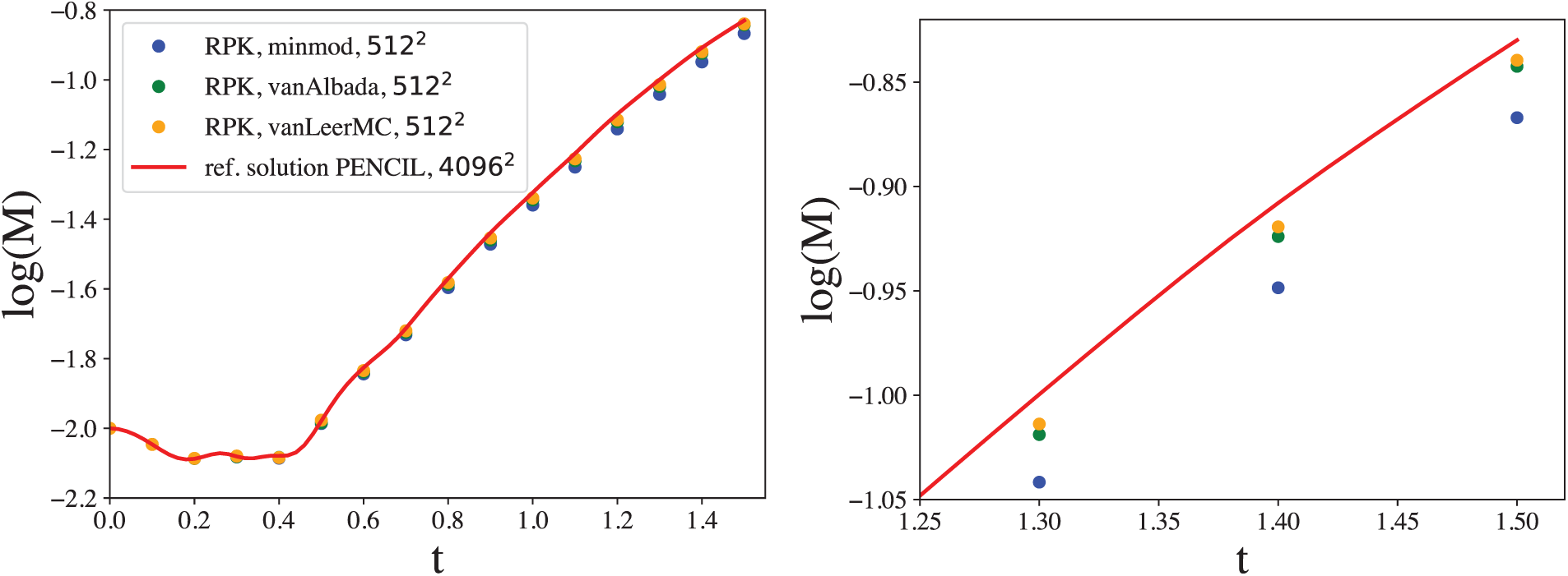
Figure 17: The growth of the Kelvin-Helmholtz instability for different slope limiters (at 5122) is shown in the left panel, a zoom-in is shown on the right

3.5 Cylindrical Kelvin-Helmholtz Instability

As a variant of the Kelvin-Helmholtz instability, we also perform a test in cylindrical symmetry, similar to [66]. To this end, we place particles from a radius of RBD1=0.5 to RBD2=1.5. For the region with r<1, we use

ρ=1ω=2P=4+2r2,(62)

and we also use

ρ=2ω=1P=5+r2,(63)

where ω is the angular frequency. In addition, we impose a small radial velocity perturbation on the interface given by

vr=v0cos⁡(10 φ) e−(r−1)22σ02,(64)

where φ is the azimuthal angle, v0=0.02 and σ0=0.1.

In our initial setup, we placed 1.95 million particles in a uniform, close-packed lattice so that the particles have the above properties. Again, we use the full 3D code to simulate a slice with 20 layers of particles in the z-direction, we do not allow for motion in the z-direction, and we enforce the above velocities within RBD1 and RBD1+0.05 and RBD2−0.05 and RBD2 as boundary conditions.

We show in Fig. 18 the density at t=2.2, again for our three limiters. There are small artefacts at the inner and outer boundaries because of our simple treatment of the boundary conditions, but in all cases, we see healthy growing Kelvin-Helmholtz instabilities with nicely winding billows. For the most diffusive limiter (minmod), we see essentially only the triggered modes growing. In contrast, in the other two cases, “parasitic” modes have also developed, which have been triggered by the granularity of our closely-packed particles shearing against each other.

Figure 18: Density in cylindrical Kelvin-Helmholtz test for the different slope limiters

3.6 Rayleigh-Taylor Instability

The Rayleigh-Taylor instability is a standard probe of the subsonic growth of a small perturbation. In its simplest form, a density layer ρt rests on top of a layer with density ρb<ρt in a constant acceleration field, e.g., due to gravity. While the denser fluid sinks down, it develops a characteristic “mushroom-like” pattern. Simulations with traditional SPH implementations have shown only retarded growth or even complete suppression of instability [67,68].

We again adopt a quasi-2D setup and use the full 3D code for the evolution. We place the particles on a cubic lattice in the xy-domain [−0.25,0.25]×[0,1] and use 20 layers of particles in the z-direction, and also place 20 layers of particles as boundaries around this core region. The properties of particles below y=0 are “frozen” at the values of the initial conditions, for particles with ya>1, we multiply a damping factor

ξ=exp⁡{−(ya−10.05)2},(65)

to the temporal derivatives so that any evolution in this upper region is strongly suppressed. We apply periodic boundaries in x− direction at x=±0.25. Similar to [20] we use ρt=2, ρb=1, a constant acceleration g→=−0.5e^y and

ρ(y)=ρb+ρt−ρb1+exp⁡[−(y−yt)/Δ],(66)

with transition width Δ=0.025 and transition coordinate yt=0.5. We apply a small velocity perturbation to the interface

vy(x,y)=δvy,0[1+cos⁡(8πx)][1+cos⁡(5π(y−yt))],(67)

for y in [0.3,0.7] with an initial amplitude δvy,0=0.025, and we use a polytropic equation of state with exponent Γ=1.4. The equilibrium pressure profile is given by

P(y)=P0−gρ(y)[y−yt],(68)

with P0=ρt/Γ, so that the sound speed is near unity in the transition region.

We show in Fig. 19 the results for different resolutions at t=4 for the vanAlbada limiter. At all resolutions, the instability grows and reaches similar y values, but, of course, with finer detailed structures for higher resolution. In Fig. 20, we show the medium resolution case for the different limiters, again confirming the hierarchy of dissipation levels with minmod being the most and vanLeerMC being the least dissipative limiter.

Figure 19: Rayleigh-Taylor instability test (at t = 4) with vanAlbada limiter at different resolution: 1282 (left), 2562 (middle) and 5122 (right)

Figure 20: Rayleigh-Taylor instability test (at t = 4.3) with 2562 particles and different slope limiters

3.7 Complex Shocks with Vorticity Creation

Schulz-Rinne [43] suggested a set of very challenging 2D benchmark tests. The tests are constructed so that four constant states meet at one corner, and the initial values are chosen so that an elementary wave, either a shock, a rarefaction, or a contact discontinuity, appears at each interface. During subsequent evolution, complex wave patterns emerge for which exact solutions are not known. These tests are considered very challenging benchmarks for multidimensional hydrodynamic codes [43,69–71]. Such tests have rarely been shown for SPH. We are only aware of the work by [26], who show results for one such shock test in a study of Godunov SPH with approximate Riemann solvers and as benchmarks for the MAGMA2 code [21].

Here, we investigate three such configurations. We simulate, as before, a 3D slice thick enough so that the midplane is unaffected by edge effects (we use 20 particle layers in z-direction). We place particles on a cubic lattice so that 300 × 300 particles are within [xc−0.3,xc+0.3]×[yc−0.3,yc+0.3], where (xc,yc) is the contact point of the quadrants, and we use a polytropic exponent Γ=1.4 in all tests. We refer to these Schulz-Rinne type problems as SR1-SR3 and give their initial parameters for each quadrant in Table 2. These test problems correspond to configurations 3, 11, and 12 in the labeling convention of [70]. We smooth the initial conditions through ⟨A⟩a=∑b[(mb/ρb)AbWab]/[∑b(mb/ρb)Wab] so that they have a smoothness that is consistent with the evolution code.

For all three tests, we find very good agreement with the results published in the literature [43,69–71,21]. Comparing the performance of the different limiters for test SR1 (first row in Fig. 21), we see only minor differences. All cases nicely produce the shock surfaces and all show the “mushroom-like” structure near (0.2, 0.2) with only small differences. The structure around (0.3, 0.3), however, does show some differences: it looks “mushroom-like” for the least dissipative case (vanLeerMC), but not very much so for the more dissipative limiters. Also, test SR2 agrees overall well with the results in the literature, but here the “mushroom-like” structures are different: the curls show more windings for lower dissipation, that is, the smallest number for minmod and the highest for vanLeerMC. The SR3 test also agrees well with the results in the literature, here the results for the different limiters are virtually identical.

Figure 21: Schulz-Rinne test 1 (first row), test 2 (second row), and test 3 (third row), color-coded is the density. The first column each time refers to minmod, the second to vanAlbada and the third one to vanLeerMC

4  Conclusion

Here, we have presented and explored a new formulation of particle hydrodynamics. We started from a common SPH formulation and enhanced it with Roe’s approximate Riemann solver to solve Riemann problems between interacting particle pairs. More specifically, we replaced the mean values of the pressures and (projected) velocities with the contact discontinuity values P∗ and v∗. We identified the terms in the Roe solver that are responsible for the dissipation. In these terms, we replaced the particle properties with the values found by slope-limited reconstruction from both sides to the interparticle midpoint. We use kernels that are designed to enforce consistency relations and which, by construction, recover constant and linear functions to machine precision, called “reproducing kernels”. We have carefully scrutinized our corresponding implementation based on a “glass-like” particle distribution, and we compare the function and gradient reproduction to the standard SPH approximation. We find that the errors in this test are at least nine orders of magnitude lower for the RPK than for the standard SPH approach. These reproducing kernels are used both for the hydrodynamic gradients and in the reconstruction process.

We have put our new formulation to the test in many challenging benchmarks, ranging from shocks over instabilities to vorticity-creating shock tests designed by Schulz-Rinne. We find very good results in all tests and, where comparable, we find slightly better but overall very similar results to the MAGMA2 code. We have also explored three different slope limiters in the reconstruction: minmod, vanAlbada, and vanLeerMC. Although minmod is an overall robust choice, it leads to more dissipation than appears necessary. The vanLeerMC limiter, in contrast, produces the least dissipation of the three limiters, but maybe not enough in the Sedov blast wave test, where it leads to substantially more post-shock noise than the other limiters, and an overshoot of the density. Of the three explored limiters, our clear favorite is the vanAlbada limiter, which performs well in all tests, but it may be worth exploring further limiters in the future. Although the results presented are very encouraging, more work needs to be done. This may include further studies of robustness and accuracy, a careful comparison with modern SPH formulations, and the inclusion of additional physics. However, these explorations are left for future work.

Acknowledgement: The simulations for this paper have been performed on the facilities of North-German Supercomputing Alliance (HLRN), and at the SUNRISE HPC facility supported by the Technical Division at the Department of Physics, Stockholm University, and on the HUMMEL2 cluster funded by the Deutsche Forschungsgemeinschaft (498394658). Special thanks go to Mikica Kocic (SU), Thomas Orgis and Hinnerk Stüben (both UHH) for their excellent support. Some plots have been produced with the software splash [72].

Funding Statement: The author has been supported by the Swedish Research Council (VR) under grant number 2020-05044, by the research environment grant “Gravitational Radiation and Electromagnetic Astrophysical Transients” (GREAT) funded by the Swedish Research Council (VR) under Dnr 2016-06012, by the Knut and Alice Wallenberg Foundation under grant Dnr. KAW 2019.0112, by the Deutsche Forschungsgemeinschaft (DFG, German Research Foundation) under Germany’s Excellence Strategy-EXC 2121 “Quantum Universe”-390833306 and by the European Research Council (ERC) Advanced Grant INSPIRATION under the European Union’s Horizon 2020 Research and Innovation Programme (Grant agreement No. 101053985).

Availability of Data and Materials: The data underlying this article will be shared on reasonable request to the corresponding author.

Ethics Approval: Not applicable.

Conflicts of Interest: The author declares no conflicts of interest to report regarding the present study.

1For the publication [21], the author collected in the computational astrophysics community a large set of test problems “that SPH cannot do”, but please see the (excellent) results in this paper.

References

1. Lucy LB. A numerical approach to the testing of the fission hypothesis. Astron J. 1977;82:1013. doi:10.1086/112164. [Google Scholar] [CrossRef]

2. Gingold RA, Monaghan JJ. Smoothed particle hydrodynamics: theory and application to non-spherical stars. Mon Not R Astron Soc. 1977;181(3):375–89. doi:10.1093/mnras/181.3.375. [Google Scholar] [CrossRef]

3. Xu X, Jiang Y-L, Yu P. SPH simulations of 3D dam-break flow against various forms of the obstacle. Ocean Eng. 2021;229(2):108978. doi:10.1016/j.oceaneng.2021.108978. [Google Scholar] [CrossRef]

4. Rahimi MN, Moutsanidis G. A smoothed particle hydrodynamics approach for phase field modeling of brittle fracture. Comput Methods Appl Mech Eng. 2022;398(3):115191. doi:10.1016/j.cma.2022.115191. [Google Scholar] [CrossRef]

5. Monaghan JJ. Smoothed particle hydrodynamics and its diverse applications. Annu Rev Fluid Mech. 2012;44(1):323–46. doi:10.1146/annurev-fluid-120710-101220. [Google Scholar] [CrossRef]

6. Rosswog S. Modelling astrophysical fluids with particles. In: Bisikalo D, Wiebe D, Boily C, editors. The predictive power of computational astrophysics as a discover tool. Cambridge, UK: Cambridge University Press; 2023. p. 382–97. doi:10.1017/s1743921322001600. [Google Scholar] [CrossRef]

7. Monaghan JJ. Smoothed particle hydrodynamics. Rep Prog Phys. 2005;68:1703–59. [Google Scholar]

8. Rosswog S. Astrophysical smooth particle hydrodynamics. New Astron Revi. 2009;53(4-6):78–104. doi:10.1016/j.newar.2009.08.007. [Google Scholar] [CrossRef]

9. Springel V. Smoothed particle hydrodynamics in astrophysics. ARAA. 2010;48:391–430. [Google Scholar]

10. Price DJ. Smoothed particle hydrodynamics and magnetohydrodynamics. J Comput Phys. 2012;231(3):759–94. doi:10.1016/j.jcp.2010.12.011. [Google Scholar] [CrossRef]

11. Rosswog S. SPH methods in the modelling of compact objects. Living Rev Computat Astrophy. 2015;1(1):1. doi:10.1007/lrca-2015-1. [Google Scholar] [CrossRef]

12. Rosswog S, Diener P. SPHINCS_BSSN: a general relativistic smooth particle hydrodynamics code for dynamical spacetimes. Class Quantum Gravity. 2021;38(11):115002. doi:10.1088/1361-6382/abee65. [Google Scholar] [CrossRef]

13. Rosswog S, Torsello F, Diener P. The Lagrangian Numerical Relativity code SPHINCS_BSSN_v1.0. Front Appl Math Stat. 2023;9:161101. doi:10.3389/fams.2023.1236586. [Google Scholar] [CrossRef]

14. Rosswog S, Diener P. Sphincs_bssn: numerical relativity with particles. In: Bambi C, Mizuno Y, Shashank S, Yuan F, editors. New frontiers in GRMHD simulations. Singapore: Springer; 2025. doi:10.1007/978-981-97-8522-3. [Google Scholar] [CrossRef]

15. Morris JP, Monaghan JJ. A switch to reduce sph viscosity. J Comp Phys. 1997;136:41. doi:10.1006/jcph.1997.5690. [Google Scholar] [CrossRef]

16. Rosswog S, Davies MB, Thielemann F-K, Piran T. Merging neutron stars: asymmetric systems. A&A. 2000;360:171–84. doi:10.48550/arXiv.astro-ph/0005550. [Google Scholar] [CrossRef]

17. Cullen L, Dehnen W. Inviscid smoothed particle hydrodynamics. MNRAS. 2010;408(2):669–83. doi:10.1111/j.1365-2966.2010.17158.x. [Google Scholar] [CrossRef]

18. Rosswog S. Boosting the accuracy of SPH techniques: newtonian and special-relativistic tests. MNRAS. 2015;448(4):3628–64. doi:10.1093/mnras/stv225. [Google Scholar] [CrossRef]

19. Rosswog S. A simple, entropy-based dissipation trigger for SPH. ApJ. 2020;898(1):60. doi:10.3847/1538-4357/ab9a2e. [Google Scholar] [CrossRef]

20. Frontiere N, Raskin CD, Owen JM. CRKSPH-a conservative reproducing kernel smoothed particle hydrodynamics scheme. J Comput Phys. 2017;332(3):160–209. doi:10.1016/j.jcp.2016.12.004. [Google Scholar] [CrossRef]

21. Rosswog S. The Lagrangian hydrodynamics code MAGMA2. MNRAS. 2020;498(3):4230–55. doi:10.1093/mnras/staa2591. [Google Scholar] [CrossRef]

22. Sandnes TD, Eke VR, Kegerreis JA, Massey RJ, Ruiz-Bonilla S, Schaller M, et al. REMIX SPH–improving mixing in smoothed particle hydrodynamics simulations using a generalised, material-independent approach. arXiv:2407.18587. 2024. [Google Scholar]

23. Inutsuka S-I. Reformulation of smoothed particle hydrodynamics with Riemann solver. J Comput Phys. 2002;179(1):238–67. doi:10.1006/jcph.2002.7053. [Google Scholar] [CrossRef]

24. Parshikov AN, Medin SA. Smoothed particle hydrodynamics using interparticle contact algorithms. J Comput Phys. 2002;180(1):358–82. doi:10.1006/jcph.2002.7099. [Google Scholar] [CrossRef]

25. Sirotkin FV, Yoh JK. A Smoothed Particle Hydrodynamics method with approximate Riemann solvers for simulation of strong explosions. Comput Fluids. 2013;88:418–29. doi:10.1016/j.compfluid.2013.09.029. [Google Scholar] [CrossRef]

26. Puri K, Ramachandran P. Approximate Riemann solvers for the Godunov SPH (GSPH). J Comput Phys. 2014;270(2):432–58. doi:10.1016/j.jcp.2014.03.055. [Google Scholar] [CrossRef]

27. Meng ZF, Zhang AM, Wang PP, Ming FR. A shock-capturing scheme with a novel limiter for compressible flows solved by smoothed particle hydrodynamics. Comput Methods Appl Mech Eng. 2021;386(420):114082. doi:10.1016/j.cma.2021.114082. [Google Scholar] [CrossRef]

28. Wendland H. Piecewise polynomial, positive definite and compactly supported radial functions of minimal degree. Adv Comput Math. 1995;4(1):389–96. doi:10.1007/bf02123482. [Google Scholar] [CrossRef]

29. Cabezon RM, Garcia-Senz D, Relano A. A one-parameter family of interpolating kernels for smoothed particle hydrodynamics studies. J Comput Phys. 2008;227(19):8523–40. doi:10.1016/j.jcp.2008.06.014. [Google Scholar] [CrossRef]

30. Dehnen W, Aly H. Improving convergence in smoothed particle hydrodynamics simulations without pairing instability. MNRAS. 2012;425(2):1068–82. doi:10.1111/j.1365-2966.2012.21439.x. [Google Scholar] [CrossRef]

31. Garcia-Senz D, Cabezon R, Escartin JA. Improving smoothed particle hydrodynamics with an integral approach to calculating gradients. A & A. 2012;538:A9. doi:10.1051/0004-6361/201117939. [Google Scholar] [CrossRef]

32. Cabezon RM, Garcia-Senz D, Escartin JA. Testing the concept of integral approach to derivatives within the smoothed particle hydrodynamics technique in astrophysical scenarios. A & A. 2012;545:A112. doi:10.1051/0004-6361/201219821. [Google Scholar] [CrossRef]

33. Antona R, Vacondio R, Avesani D, Righetti M, Renzi M. Towards a high order convergent ale_sph scheme with efficient weno spatial reconstruction. Water. 2021;13(17):2432. doi:10.3390/w13172432. [Google Scholar] [CrossRef]

34. Avesani D, Dumbser M, Vacondio R, Righetti M. An alternative SPH formulation: ADER-WENO-SPH. Comput Methods Appl Mech Eng. 2021;382(3):113871. doi:10.1016/j.cma.2021.113871. [Google Scholar] [CrossRef]

35. Vergnaud A, Oger G, Le Touzé D. Investigations on a high order SPH scheme using WENO reconstruction. J Comput Phys. 2023;477(17):111889. doi:10.1016/j.jcp.2022.111889. [Google Scholar] [CrossRef]

36. Antona R, Vacondio R, Avesani D, Righetti M, Renzi M. A WENO SPH scheme with improved transport velocity and consistent divergence operator. Comput Part Mech. 2024;11(3):1221–40. doi:10.1007/s40571-023-00681-z. [Google Scholar] [CrossRef]

37. Moussa BB, Lanson N, Vila JP. Convergence of meshless methods for conservation laws: applications to Euler equations. Int Ser Num Mathem. 1999;129(3):31–40. doi:10.1007/978-3-0348-8720-5_4. [Google Scholar] [CrossRef]

38. Vila JP. On particle weighted methods and smooth particle hydrodynamics. Mathemat Mod Meth Appl Sci. 1999;2(2):161–209. doi:10.1142/s0218202599000117. [Google Scholar] [CrossRef]

39. Hietel D, Steiner K, Struckmeier J. A finite-volume particle method for compressible flows. Math Model Methods Appl Sci. 2000;10(9):1363–82. doi:10.1142/s0218202500000604. [Google Scholar] [CrossRef]

40. Junk M. Do finite volume methods need a mesh? In: Griebel M, Schweitzer MA, editors. Meshfree methods for partial differential equations. Lecture notes in computational science and engineering. Berlin/Heidelberg: Springer; 2003. Vol. 26. p. 223–38. doi:10.1007/978-3-642-56103-0_15. [Google Scholar] [CrossRef]

41. Gaburov E, Nitadori K. Astrophysical weighted particle magnetohydrodynamics. MNRAS. 2011 Jun;414(1):129–54. doi:10.1111/j.1365-2966.2011.18313.x. [Google Scholar] [CrossRef]

42. Ramírez L, Eirís A, Couceiro I, París J, Nogueira X. An arbitrary Lagrangian-Eulerian SPH-MLS method for the computation of compressible viscous flows. J Comput Phys. 2022;464(2):111172. doi:10.1016/j.jcp.2022.111172. [Google Scholar] [CrossRef]

43. Schulz-Rinne CW. Classification of the Riemann problem for two-dimensional gas dynamics. SIAM J Mathem Analy. 1993;24(1):76–88. doi:10.1137/0524006. [Google Scholar] [CrossRef]

44. Liu GR, Liu MB. Smoothed particle hydrodynamics: a meshfree particle method. Singapore: World Scientific; 2003. [Google Scholar]

45. Rosswog S, Diener P, Torsello F. Thinking outside the box: numerical relativity with particles. Symmetry. 2022;14(6):1280. doi:10.3390/sym14061280. [Google Scholar] [CrossRef]

46. Toro EF. Riemann solvers and Numerical methods for fluid dynamics. 3rd ed. Berlin, Germany: Springer-Verlag; 2009. [Google Scholar]

47. Roe PL. Characteristic-based schemes for the Euler equations. Annu Rev Fluid Mech. 1986;18(1):337–65. doi:10.1146/annurev.fl.18.010186.002005. [Google Scholar] [CrossRef]

48. Van Leer B. Towards the ultimate conservative difference scheme. IV. A new approach to numerical convection. J Comput Phys. 1977;23(3):276–99. doi:10.1016/0021-9991(77)90095-x. [Google Scholar] [CrossRef]

49. van Albada GD, van Leer B, Roberts WW Jr. A comparative study of computational methods in cosmic gas dynamics. A & A. 1982;108(1):76–84. [Google Scholar]

50. Liu WK, Jun S, Zhang YF. Reproducing kernel particle methods. Int J Numer Methods Fluids. 1995;20(8–9):1081–106. doi:10.1002/fld.1650200824. [Google Scholar] [CrossRef]

51. Du Q, Wang D. The optimal centroidal voronoi tessellations and the gersho’s conjecture in the three-dimensional space. Comput Mathemat Applicat. 2005;49(9–10):1355–73. doi:10.1016/j.camwa.2004.12.008. [Google Scholar] [CrossRef]

52. Gafton E, Rosswog S. A fast recursive coordinate bisection tree for neighbour search and gravity. MNRAS. 2011;418:770–81. doi:10.1111/j.1365-2966.2011.19528.x. [Google Scholar] [CrossRef]

53. Gottlieb S, Shu CW. Total variation diminishing Runge-Kutta schemes. Math Comput. 1998;67:73–85. doi:10.1090/s0025-5718-98-00913-2. [Google Scholar] [CrossRef]

54. Owen JM. A compatibly differenced total energy conserving form of SPH. Numer Meth Fluids. 2014;75:749–74. doi:10.1002/fld.3912. [Google Scholar] [CrossRef]

55. Cercos-Pita JL, Merino-Alonso PE, Calderon-Sanchez J, Duque D. The role of time integration in energy conservation in Smoothed Particle Hydrodynamics fluid dynamics simulations. Eur J Mech, B/Fluids. 2023;97:78–92. doi:10.1016/j.euromechflu.2022.09.001. [Google Scholar] [CrossRef]

56. Sedov LI. Similarity and dimensional methods in mechanics. New York, NY, USA: Academic Press; 1959. [Google Scholar]

57. Taylor G. The formation of a blast wave by a very intense explosion. I. Theoretical discussion. Proc Royal Soc London Ser A. 1950;201:159–74. doi:10.1098/rspa.1950.0049. [Google Scholar] [CrossRef]

58. Casanova J, Jose J, Garcia-Berro E, Shore SN, Calder AC. Kelvin-Helmholtz instabilities as the source of inhomogeneous mixing in nova explosions. Nature. 2011;478(7370):490–2. doi:10.1038/nature10520. [Google Scholar] [PubMed] [CrossRef]

59. Price DJ, Rosswog S. Producing ultra-strong magnetic fields in neutron star mergers. Science. 2006;312:719–22. doi:10.1126/science.1125201. [Google Scholar] [PubMed] [CrossRef]

60. Giacomazzo B, Zrake J, Duffell PC, MacFadyen AI, Perna R. Producing magnetar magnetic fields in the merger of binary neutron stars. ApJ. 2015;809(1):39. doi:10.1088/0004-637x/809/1/39. [Google Scholar] [CrossRef]

61. Kiuchi K, Cerdá-Durán P, Kyutoku K, Sekiguchi Y, Shibata. M. Efficient magnetic-field amplification due to the Kelvin-Helmholtz instability in binary neutron star mergers. Phys Rev D. 2015;92(12):124034. doi:10.1103/physrevd.92.124034. [Google Scholar] [CrossRef]

62. Johnson JR, Wing S, Delamere PA. Kelvin helmholtz instability in planetary magnetospheres. Space Sci Rev. 2014;184(1–4):1–31. doi:10.1007/s11214-014-0085-z. [Google Scholar] [CrossRef]

63. Agertz O, Moore B, Stadel J, Potter D, Miniati F, Read J, et al. Fundamental differences between SPH and grid methods. MNRAS. 2007;380(3):963–78. doi:10.1111/j.1365-2966.2007.12183.x. [Google Scholar] [CrossRef]

64. McNally CP, Lyra W, Passy J-C. A well-posed kelvin-helmholtz instability test and comparison. ApJS. 2012;201:18. doi:10.1088/0067-0049/201/2/18. [Google Scholar] [CrossRef]

65. Brandenburg A, Dobler W. Hydromagnetic turbulence in computer simulations. Comput Phys Commun. 2002;147(1–2):471–5. doi:10.1016/s0010-4655(02)00334-x. [Google Scholar] [CrossRef]

66. Duffell PC. DISCO: a 3D moving-mesh magnetohydrodynamics code designed for the study of astrophysical disks. Ap J Supp. 2016;226(1):2. doi:10.3847/0067-0049/226/1/2. [Google Scholar] [CrossRef]

67. Abel T. rpSPH: a novel smoothed particle hydrodynamics algorithm. MNRAS. 2011;413(1):271–85. doi:10.1111/j.1365-2966.2010.18133.x. [Google Scholar] [CrossRef]

68. Saitoh TR, Makino J. A density-independent formulation of smoothed particle hydrodynamics. ApJ. 2013;768(1):44. doi:10.1088/0004-637x/768/1/44. [Google Scholar] [CrossRef]

69. Lax P, Liu XD. Solution of two-dimensional Riemann problems of gas dynamics by positive schemes. SIAM J Sci Comput. 1998;19(2):319–40. doi:10.1137/s1064827595291819. [Google Scholar] [CrossRef]

70. Kurganov A, Tadmor E. Solution of two-dimensional riemann problems for gas dynamics without riemann problem solvers. Numer Methods Partial Differ Equ. 2002;18(5):584–608. doi:10.1002/num.10025. [Google Scholar] [CrossRef]

71. Liska R, Wendroff B. Comparison of several difference schemes on 1D and 2D test problems for the euler equations. SIAM J Sci Comput. 2003;25(3):995–1017. doi:10.1137/s1064827502402120. [Google Scholar] [CrossRef]

72. Price DJ. splash: an interactive visualisation tool for smoothed particle hydrodynamics simulations. Publ Astron Soc Aust. 2007;24(3):159–73. doi:10.1071/as07022. [Google Scholar] [CrossRef]