Average Run Length in TEWMA Control Charts: Analytical Solutions for AR(p) Processes and Real Data Applications

1  Introduction

The Fredholm integral equation plays a crucial role in various fields of mathematics and science, including physics, engineering mathematics, and signal analysis. It is a type of linear integral equation that can be categorized into two distinct forms: the first and the second kind. These two forms differ in structure and methods of solving them. One notable application of the second-kind Fredholm equation is in determining the Average Run Length (ARL) of control charts. The ARL is an important performance metric used to assess control charts, as it represents the average number of observations needed before a signal is triggered. The ARL has two key values: ARL0, which indicates the expected number of observations before a control chart detects that the process is out of control, and ARL1, which indicates the expected number of observations required when the process is actually out of control. Several methods have been proposed for calculating the ARL value of control charts, including approaches based on Markov chains, martingales, Monte Carlo simulations, explicit formulas, and numerical integral equations (NIEs). The Fredholm integral equation, characterized by a kernel function with constant integration limits, shares similarities with the Volterra integral equation, which has variable integration limits. The second kind of Fredholm integral equation is particularly significant in mathematical analysis and finds applications across various scientific fields. Solutions to these equations can be derived using iterative or analytical methods, with explicit formulas providing direct solutions for calculating the Average Run Length (ARL) [1,2]. Crowder [3] pioneered the application of second-kind Fredholm equations to EWMA charts, while Champ and Rigdon [4] extended this approach to the cumulative sum chart. Studies on explicit ARL formulas and numerical integral equations (NIEs) have since been conducted by several researchers [5–9], employing methods such as the midpoint, trapezoidal, Simpson’s, Boole’s, and Gauss-Legendre rules. For instance, Peerajit et al. [10] used the Gauss-Legendre quadrature to approximate ARL in CUSUM charts under long-memory processes, while Peerajit [11] applied NIEs to detect mean shifts in similar settings. Phanyaem [12] developed explicit formulas and NIEs for evaluating ARL of cumulative sum chart for a seasonal autoregressive with exogenous variable, ARX (P,r)L models, and Makaew et al. [13] utilized NIEs to analyze ARL for TEWMA charts in autoregressive processes. Peerajit [14] further applied NIEs for ARL approximation in EWMA charts for the fractionally integrated AR model with an exogenous variable (ARFIX) using the Gauss-Legendre quadrature. This study employs the trapezoidal rule for NIE approximations.

In Statistical Process Control (SPC), control charts are key tools for monitoring and maintaining process stability. Introduced by Shewhart [15], control charts visually track process data over time to detect trends or anomalies, ensuring consistency and quality. The Shewhart chart effectively identifies large shifts, while Page’s [16] cumulative sum (CUSUM) chart is better suited for smaller shifts. Similarly, Robert [17] introduced the exponentially weighted moving average (EWMA) chart to enhance small-shift detection. Subsequent refinements include Shamma and Shamma [18] double EWMA (DEWMA) chart and Alevizakos et al.’s [19] triple EWMA (TEWMA) chart, designed for normally distributed data. Recent studies, such as those by Chatterjee [20,21], Supharakonsakun and Areepong [22], and Karoon et al. [23], have advanced ARL analysis for time series and moving average processes under these frameworks. Alevizakos et al. [24,25] further explored TEWMA charts, comparing various weighted moving average models to highlight the advantages of double, triple, and quadruple EWMA approaches. More recently, Hu et al. [26] proposed a Triple Exponentially Weighted Moving Average (TEWMA) control chart with a Variable Sampling Interval (VSI) feature to monitor the coefficient of variation (CV). Additional research on DEWMA and TEWMA control charts, as seen in [27–31], has further expanded the understanding and application of these charts in diverse quality control contexts.

Typically, EWMA and TEWMA control charts include both upper and lower control limits, making them essential tools for quality management. However, our research specifically focuses on one-sided criteria, specifically upper control limits. For manufacturing situations, the application of upper control limits has only shown its efficacy in the quick detection of production process problems. Companies can optimize resource allocation and provide consistent product quality by finding deviations from normal standards and tackling them before they escalate.

This study aims to develop an explicit formula for calculating the Average Run Length (ARL) of the autoregressive models of order p with exponential white noise under the TEWMA control chart framework. The existence and uniqueness of the solution will be demonstrated using Banach’s fixed-point theorem and Hölder’s inequality. Simulations will compare the performance of the explicit and NIE approaches for the TEWMA control chart, as well as evaluate the effectiveness of EWMA and TEWMA charts in detecting shifts in the AR(p) model. Finally, real-world data will be analyzed to assess the performance of both EWMA and TEWMA control charts for the AR(p) process.

2  Materials and Methods

The properties related to the AR(p) model, the EWMA control chart, and the TEWMA control chart are as follows.

2.1 Autoregressive Process

The Autoregressive (AR) process is a commonly used statistical tool for analyzing time series data. It forecasts the current value of a variable as a linear combination of its previous values (lags) along with a random error term. An AR model of order p, commonly written as AR(p), is described by the following equation:

Xt=ω+ξ1Xt−1+ξ2Xt−2+…+ξpXt−p+εt,(1)

where ξi,i=1,2,…,p are coefficient parameters of the AR process (|ξi| < 1), ω is the constant and εt is the error term of the model, which is distributed as an exponential white noise, εt∼Exp(β).

2.2 The EWMA Control Chart

The EWMA control charts are often used in quality control because they allow for the early detection of small changes in process performance. The EWMA control chart is defined as follows:

Et=λXt+(1−λ)Et−1,(2)

where λ is a parameter constrained within the range 0<λ≤1. Here, Xt represents the observations from the AR(p) process and E0=μ0 is defined as the initial value. The stop time for EWMA control charts is defined as follows:

τh=inf{t > 0;Et < gorEt > h},(3)

where g denotes the lower control limit, and h represents the upper control limit. The average run length (ARL) for the EWMA control chart on the AR(p) process, given an initial value of E0=u, is expressed as follows:

H(u)=ARL=E∞(τh)≥T,E0=u,(4)

where T represents a fixed constant and E∞(.) denotes the expectation based on the assumption that observation εt follows the specified distribution. The mean and variance of the EWMA control chart are defined as E(Et)=μ and Var(Et)=(λ2−λ)σ2, respectively. The lower and the upper control limits for the EWMA control chart can be expressed as follows:

UCL=μ0+L1σλ(2−λ),LCL=μ0−L1σλ(2−λ),(5)

where the mean and the standard deviation of the process are defined as μ0, σ, respectively, and L1 is a control width parameter.

2.3 The TEWMA Control Chart

One of the control charts developed from the EWMA control chart is the triple EWMA (TEWMA). The TEWMA control chart is defined as follows:

{Et=λXt+(1−λ)Et−1,Yt=λEt+(1−λ)Yt−1,TEt=λYt+(1−λ)Wt−1,(6)

where λ is a parameter constrained within the range 0 < λ≤1. Here, Xt represents observations from the AR(p) process. The initial value is given as E0=Y0=TE0=μ0. The stop time for the TEWMA control charts is defined as follows:

τh=inf{t>0;TEt<gorTEt>h},(7)

where g denotes the lower control limit, and h represents the upper control limit. The average run length (ARL) for the TEWMA control chart on the AR(p) process, given an initial value of TE0=u, is expressed as follows:

H(u)=ARL=E∞(τh)≥T,TE0=u,(8)

where T represents a fixed constant and E∞(.) denotes the expectation based on the assumption that observation εt follows the specified distribution. The mean and variance of the EWMA control chart are defined as E(TEt)=μ, and Var(TEt)=(6(1−λ)6λ(2−λ)5+12(1−λ)4λ2(2−λ)4+7(1−λ)2λ3(2−λ)3+λ4(2−λ)2)σ2, respectively. The lower and the upper control limits for the TEWMA control chart can be expressed as follows:

UCL=μ0+L2σ6(1−λ)6λ(2−λ)5+12(1−λ)4λ2(2−λ)4+7(1−λ)2λ3(2−λ)3+λ4(2−λ)2,LCL=μ0−L2σ6(1−λ)6λ(2−λ)5+12(1−λ)4λ2(2−λ)4+7(1−λ)2λ3(2−λ)3+λ4(2−λ)2,(9)

where the mean and the standard deviation of the process are defined as μ0, σ, respectively, and L2 is a control width parameter.

3  Explicit Formula for Solving the ARL

This section outlines the derivation of the explicit formula for the ARL of the TEWMA control chart applied to the AR model. The observations are assumed to follow an AR(p) process with exponentially distributed noise. The existence and uniqueness of the ARL solutions are then verified as detailed below. From Eq. (6), the recursive formula of TEWMA statistics can be written as follows:

TEt=λ3Xt+λ2(1−λ)Et−1+λ(1−λ)Yt−1+(1−λ)TEt−1(10)

Let Xt is observation on AR(p) model, then:

TEt=λ3[ω+∑i=1pξiXt−p+εt]+λ2(1−λ)Et−1+λ(1−λ)Yt−1+(1−λ)TEt−1(11)

For t = 1, we obtain:

TE1=λ3[ω+∑i=1pξiX1−p+ε1]+λ2(1−λ)E0+λ(1−λ)Y0+(1−λ)TE0=M+λ3ε1+(1−λ)u,

where M=λ3[ω+∑i=1pξiX1−p]+λ2(1−λ)E0+λ(1−λ)Y0,0 < λ≤1 and TE0=u.

Consider a one-sided case for the in-control process, that is 0≤TEt≤h, where LCL=0 and UCL=h. So that, 0≤M+λ3ε1+(1−λ)u≤h.

Next, it rearranged into the form of ε1, we get that:

−(1−λ)u−Mλ3≤ε1≤h−(1−λ)u−Mλ3

Based on the method introduced by Champ and Rigdon [4], derived from the second-kind Fredholm integral equation, the function H(u) can be expressed as follows:

H(u)=1+∫0h−(1−λ)u−Mλ3H[M+λ3y+(1−λ)u]f(y)dy(12)

Let W=M+λ3y+(1−λ)u, then y=W−(1−λ)u−Mλ3 and dy=1λ3dW. By changing the integral variable, Eq. (12) can be written as:

H(u)=1+1λ3∫0hH[W]f(W−(1−λ)u−Mλ3)dW(13)

Since ε1∼Exp(β), then f(x)=1βe−xβ;x≥0. Thus:

H(u)=1+e(1−λ)u+Mβλ3βλ3∫0hH(w)e−Wβλ3dW.(14)

Let Q(u)=1βλ3e(1−λ)u+Mβλ3 and R=∫0hH(W)e−Wβλ3dW, so that:

H(u)=1+Q(u)R(15)

Consider that R=∫0hH(W)e−Wβλ3dW, then:

R=∫0hH[W]e−Wβλ3dW=∫0h[1+Q(W)R]e−Wβλ3dW=∫0he−Wβλ3dW+ReMβλ3βλ3∫0he−Wβλ2dW

So, we obtain R=−βλ3[e−hβλ3−1]1+eMβλ3λ[e−hβλ2−1].

Finally, by substituting R into Eq. (15), we obtain:

H(u)=1−e(1−λ)u+Mβλ3[e−hβλ3−1](1+eMβλ3λ[e−hβλ2−1])(16)

Under the in-control condition (β=β0), the explicit ARL0 formula for the TEWMA control chart in an AR(p) process is given by:

ARL0=1−e(1−λ)u+Mβ0λ3[e−hβ0λ3−1]1+eMβ0λ3λ[e−hβ0λ2−1].

When the process is out of control (β=β1,β1=(1+δ)β0), where δ indicates the shift size, the explicit formula for ARL1 in the TEWMA control chart for an AR(p) process is given by:

ARL1=1−e(1−λ)u+Mβ1λ3[e−hβ1λ3−1]1+eMβ1λ3λ[e−hβ1λ2−1].

Proposition 1 Banach’s Fixed-point Theorem: Suppose that H defined on a complete metric space and T:H→H be a contraction mapping on H such that:

‖T(H1)−T(H2)‖≤δ‖H1−H2‖

for:

H1,H2∈H,

then the problem has a unique solution in H [32].

Proof: Let T be a contraction mapping operator defined as follows:

T(H(u))=1+1λ3∫0nH(w)f(w−(1−λ)u−Mλ3)dw,

for any H1,H2∈C[0,h] with ‖L‖∞=supu∈[0,b]|H(u)|. First, consider:

‖T(H1(u))−T(H2(u))‖∞=supu∈[0,n]{|(1+1λ3∫0nH1(w)f(w−(1−λ)u−Mλ3)dw)−(1+1λ3∫0nH2(w)f(w−(1−λ)u−Mλ3)dw)|}=|1λ3∫0nH1(w)f(w−(1−λ)u−Mλ3)dw−1λ3∫0nH2(w)f(w−(1−λ)u−Mλ3)dw|≤1λ3∫0n‖H1(w)−H2(w)‖∞f(w−(1−λ)u−Mλ3)dw

Next, using the Hölder’s Inequality, it can be written as follows:

‖T(H1(u))−T(H2(u))‖∞≤1λ3‖H1−H2‖∞∫0nf(w−(1−λ)u−Mλ3)dw≤1λ3‖H1−H2‖∞(∫0n|f(w−(1−λ)u−Mλ3)|11−σdw)1−σ(∫0n|1|1σdw)σ≤nσλ3‖H1−H2‖∞(e(1−λ)u−Mβλ3βλ3)1−σ(βλ3(1−σ)(1−e−nβλ3(1−σ)))1−σ=nσλ3((1−σ)e(1−λ)u−Mβλ3(1−e−nβλ3(1−σ)))1−σ‖H1−H2‖∞≤δ‖H1−H2‖∞,

where δ=nσλ3((1−σ)e(1−λ)u−Mβλ3(1−e−nβλ3(1−σ)))1−σ∈[0,1), with σ,λ∈(0,1),β>0. From the assumption given above, therefore ‖T(H1(u))−T(H2(u))‖≤δ‖H1−H2‖∞, then T is the contraction mapping on complete metric space, and by the Banach fixed point theorem, T has a unique solution in H. □

4  The NIE Method for Solving the ARL

The Numerical Integral Equation (NIE) method is employed to calculate the Average Run Length (ARL) for the TEWMA control chart on the AR(p) process. This method includes various techniques such as the Midpoint Rule, Trapezoidal Rule, and Simpson’s Rule, etc. In this study, the trapezoidal rule is specifically utilized [13]. By approximating LNIE(u) through a system of m linear equations, the ARL is computed using the trapezoidal rule, as determined as follows:

LNIE(u)≈1+1λ3∑j=1mwjL(xj)f(xj−(1−λ)u−(λ3(ϕ0+ϕ1X0+…+ϕpX1−p)+λ2Y0(1−λ)+λZ0(1−λ))λ3),(17)

where xj=jwj, wj=hm,j=1,2,…,m−1. Otherwise wj=h2m.

5  Simulated Results

In this section, the efficiency performance is compared between previously proposed approximations [11] and the explicit solution obtained in this study of TEWMA charts on AR models, specifically AR(1), AR(2), and AR(3) for the determination of the average run length (ARL), where a low ARL value indicates accurate detection efficiency. In the simulations, ARL0=370 was considered. The approximation method used is the trapezoidal method with the number of iterations m = 1000. For the in-control process, the initial value is set to β0=10. On the other hand for the out-of-control process, it is set to β1=(1+δ)β0, where δ is the shift size, which is considered from very small changes and then gradually moved as follows: 0.000, 0.001, .0003, 0.005, 0.007, 0.010, 0.030, 0.050, 0.070, 0.100, 0.300, 0.500, 0.700 and 1.000. Since we consider only one-sided, i.e., the upper control limit (UCL) = h and lower control limit (LCL) = 0. The coefficient parameters for the AR(1), AR(2), and AR(3) models were set as follows: ξ1=0.1, ξ1=ξ2=0.1 and ξ1=ξ2=ξ3=0.1, respectively, with a constant (ω) set to 0. The steps of the process can be defined as follows:

Step 1: Specify ARL0, λ and the constant (ω) and coefficient parameters (ξi,i≥1) of AR(p) model.

Step 2: Specify the initial values of the process such as u,β0,X0.

Step 3: Calculate h for the explicit solution formula and the NIE formula.

Step 4: Calculate ARL1 (out-of-control process) by using h from the previous step, consider β1=(1+δ)β0 where δ is shift size.

The tool used to measure the efficiency of ARL between the estimated and the explicit solutions is measured by using the absolute percentage relative error (APRE). APRE is a measure of the accuracy of a forecast or estimate by comparing the predicted or estimated value to the actual value. APRE is calculated by finding the absolute error between the actual value and the predicted value, dividing the difference by the actual value and multiplying by 100 to express a percentage. The APRE formula is determined by:

APRE=|Actual Value−Estimated Value|Actual Value×100

A comparison of the ARL of the explicit formula with the NIE method for the TEWMA control chart, when λ=0.15, λ=0.75 for the AR(1), AR(2), and AR(3), are shown in Tables 1–3, respectively. In each table, Time (sec) indicates the computation time of the method to find the NIE solution and the computation time of the explicit solution for every shift size (δ) value is less than 0.0001.

From the results in Tables 1–3, it can be seen that the explicit and approximate solutions have very close values for all the shift sizes from small to large changes, but the explicit solution is still superior in computation time for all the shift sizes. The performance of the TEWMA control chart was evaluated by comparing it to its prototype, the EWMA control chart, using the Relative Mean Index (RMI) [25] as a performance metric. RMI is a statistical tool designed to compare the central tendency of one dataset to another, typically a reference or standard value. It quantifies the relationship between the mean of a dataset and a reference value, offering insights into the chart’s effectiveness. The RMI is calculated as follows:

RMI=1n∑i=1n[ARLi(c)−ARLi(s)ARLi(s)]

here, ARLi(c) represents the ARL of a control chart for a given shift size in row i, while ARLi(s) is the smallest ARL across all charts for the same row. A lower RMI value indicates superior performance in detecting shifts. Tables 4–6 present the comparison of ARL values for the EWMA and TEWMA control charts under various λ values (0.15, 0.50, and 0.75) applied to AR(1), AR(2), and AR(3) processes, respectively.

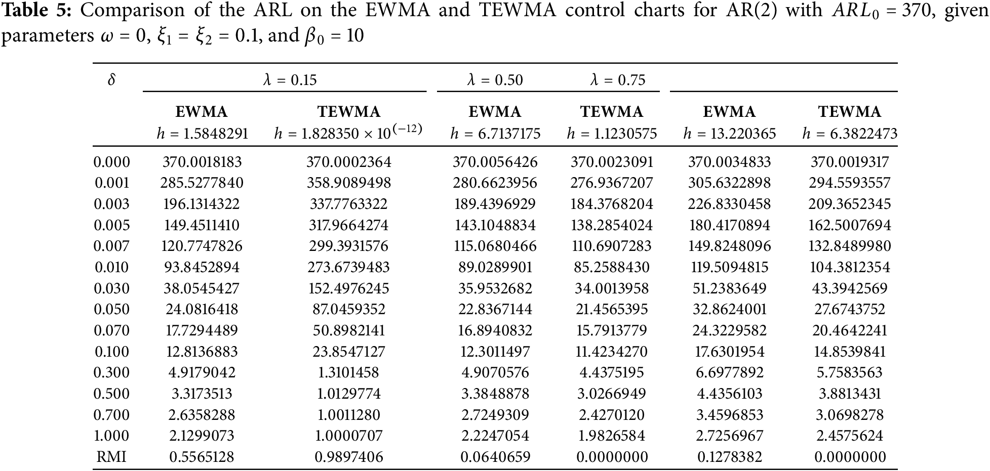
From Tables 4–6, it can be seen that the TEWMA control chart is not suitable for considering the situation with small lambda, but when the lambda value increases, the efficiency of TEWMA will increase accordingly. Moreover, the comparison between TEWMA and EWMA control charts for different ARs shown in Tables 4–6 can be further explained with graphs as shown in Fig. 1 as follows.

Figure 1: Consider RMI of EWMA and TEWMA control charts on various AR models for comparing performance when λ=0.15, λ=0.50 and λ=0.75

6  Application to Real Data

This section compares TEWMA and EWMA control charts, starting with historical data from the SET index (January–May 2024). The compatibility of the dataset with AR models—AR(1), AR(2), and AR(3)—was evaluated based on Root Mean Squared Error (RMSE), Mean Absolute Percentage Error (MAPE), and Bayesian Information Criterion (BIC), as presented in Table 7. The AR(1) model, having the lowest RMSE and BIC values, was identified as the most suitable for this dataset. Additionally, the Kolmogorov-Smirnov Test was applied to confirm the suitability of white noise conforming to the exponential mean, as shown in Table 8. The SET index for the AR(1) model can be represented as follows:

Xt=1382.234+0.918Xt−1+εt,εt∼Exp(6.8758).

Next, Table 9 presents the performance comparison between the EWMA and TEWMA control charts using previously determined real data from the AR(1) process. The steps of comparison of both control charts can be defined as follows:

Step 1: Specify ARL0 and λ.

Step 2: The dataset was tested for fit with the AR model to find the constants and coefficient parameters of the model.

Step 3: Calculate h for the EWMA and the TEWMA control charts.

Step 4: Calculate ARL1 (out-of-control process) of each control chart by using h from the previous step, considerβ1=(1+δ)β0, where δ is shift size.

From Table 9, the results are in accordance with the results in the simulation chapter, that is, the performance of TEWMA is not suitable considering a small lambda, but as the lambda increases, the performance of TEWMA will improve accordingly. In addition, Fig. 2 displays the RMI values of both control charts for AR(1), highlighting their comparative performance. Lastly, Fig. 3 illustrates the ARL values of the EWMA and TEWMA control charts for AR(1), showing the comparison across different parameters.

Figure 2: Consider RMI of EWMA and TEWMA control charts on AR(1) model for comparing performance when λ=0.15, λ=0.50 and λ=0.75

Figure 3: Comparison of the ARL between the TEWMA and the EWMA control charts for (a)λ=0.15,(b)λ=0.50, and (c)λ=0.75

From Fig. 3, it is found that the ARL value of the EWMA control chart will be higher than the TEWMA when considering the low lambda, but when the lambda value increases, the efficiency of TEWMA will increase until it is better than EWMA. Next, the performance comparison of the control charts between TEWMA and EWMA with historical data of annual global plastics production (1950–2019) is performed. Since we consider the model as AR(p), the dataset is checked for compatibility with different AR(p) models, and the exponential distribution of the error terms is examined as follows.

From Tables 10 and 11, it is found that the data set is most compatible with the AR(1) model, and the error term has an exponential distribution which can be written as follows:

Yt=137563820.884+0.999Yt−1+εt,εt∼Exp(7834147.726).

Next, Table 12 presents the performance comparison between the EWMA and TEWMA control charts using previously determined real data from the AR(1) process. In addition, Fig. 3 displays the RMI values of both control charts for AR(1), highlighting their comparative performance.

From Table 12, it can be seen that the results have the same direction as the results from the previous dataset when considering the RMI values. Then, to make it clearer, it is shown by the RMI values in Fig. 4.

Figure 4: Consider RMI of EWMA and TEWMA control charts on AR(1) model for comparing performance when λ=0.15, λ=0.50 and λ=0.75

7  Conclusion

This study evaluates the performance of control charts based on ARL. Both the explicit solution method and the numerical integral equation (NIE) method were applied to TEWMA control charts for various AR processes with exponential white noise. The efficiency of these methods was assessed in terms of APRE and computation time. The simulation results indicate that although both methods give similar results, the proposed explicit solution is less computationally intensive than the NIE method for all shift sizes. The performance of the TEWMA control chart was further compared to the EWMA control chart across different AR processes using RMI values. The results revealed that although the TEWMA chart is less effective for small λ, it outperforms the EWMA chart in detecting shifts across all shift sizes. Additionally, the comparison of TEWMA and EWMA charts was extended to real-world data, specifically the historical data of the SET index and historical data of annual global plastics production. The findings confirm that the TEWMA chart demonstrates superior performance in detecting changes compared to the EWMA chart for most λ values, consistent with the simulation results. However, a limitation of this study is that the TEWMA control chart may not perform well with small λ values, i.e., if small λ values are to be considered, the EWMA control chart is more suitable. Future research will focus on exploring TEWMA control charts or other types of control charts under different processes.

Acknowledgement: The authors confirm that this research was conducted independently by the listed authors, with no external contributors involved in any stage of the study.

Funding Statement: This research budget was allocated by the National Science, Research and Innovation Fund (NSRF), and King Mongkut’s University of Technology North Bangkok under contract no. KMUTNB-FF-68-B-08.

Author Contributions: Conceptualization, Sirawit Makaew and Yupaporn Areepong; validation, Yupaporn Areepong; methodology, Sirawit Makaew and Saowanit Sukparungsee; software, Sirawit Makaew; formal analysis, Sirawit Makaew and Saowanit Sukparungsee; investigation, Yupaporn Areepong; resources, Yupaporn Areepong; data curation, Sirawit Makaew; writing—original draft preparation, Yupaporn Areepong and Saowanit Sukparungsee; writing—review and editing, Sirawit Makaew and Yupaporn Areepong; visualization, Yupaporn Areepong; supervision, Yupaporn Areepong; funding acquisition, Yupaporn Areepong. All authors reviewed the results and approved the final version of the manuscript.

Availability of Data and Materials: The datasets used in this study are publicly available. The historical data from the SET index (January–May 2024) can be accessed at https://th.investing.com/indices/thailand-set. The historical data on annual global plastics production (1950–2019) is available at https://ourworldindata.org/grapher/global-plastics-production (accessed on 1 January 2025). No additional datasets were generated or analyzed during the study.

Ethics Approval: Not applicable.

Conflicts of Interest: The authors declare no conflicts of interest to report regarding the present study.

References

1. Knoth S, Saleh NA, Mahmoud MA, Woodall WH, Tercero-Gómez VG. A critique of a variety of “memory-based” process monitoring methods. J Qual Technol. 2023;55(1):18–42. doi:10.1080/00224065.2022.2034487. [Google Scholar] [CrossRef]

2. Li Z, Zou C, Gong Z, Wang Z. The computation of average run length and average time to signal: an overview. J Stat Comput Simul. 2014;84(8):1779–802. doi:10.1080/00949655.2013.766737. [Google Scholar] [CrossRef]

3. Crowder SV. A simple method for studying run-length distributions of exponentially weighted moving average charts. Technometrics. 1987;29(4):401–7. [Google Scholar]

4. Champ CW, Rigdon SE. A comparison of the markov chain and the integral equation approaches for evaluating the run length distribution of quality control charts. Commun Stat-Simul Comput. 1991; 20(1):191–204. doi:10.1080/03610919108812948. [Google Scholar] [CrossRef]

5. Mititelu G, Areepong Y, Sukparungsee S, Novikov A. Explicit analytical solutions for the average run length of CUSUM and EWMA charts. East-West J Math. 2010;12:253–65. [Google Scholar]

6. Raweesawat K, Sukparungsee S. Explicit formula of ARL for SMA (Q)L with exponential white noise on EWMA control chart of ZIPINAR model with an excessive number of zeros. Appl Sci Eng Prog. 2022;15(3):4588. [Google Scholar]

7. Chang YM, Wu TL. On average run lengths of control charts for autocorrelated processes. Methodol Comput Appl Probab. 2011;13(2):419–31. [Google Scholar]

8. Demirkol Akyol S, Bayhan M. ARL performances of control charts for autocorrelated data. In: Proceedings of the 38th International Conference on Computers and Industrial Engineering; 2008 Oct 31–Nov 2; Beijing, China. p. 400–8. [Google Scholar]

9. Petcharat K. Explicit formula of ARL for SMA (Q)L with exponential white noise on EWMA chart. Int J Appl Phys Math. 2016;6(4):218–25. [Google Scholar]

10. Peerajit W, Areepong Y, Sukparungsee S. Numerical integral equation method for ARL of CUSUM chart for long-memory process with non-seasonal and seasonal ARFIMA models. Thail Stat. 2018;16(1):26–37. [Google Scholar]

11. Peerajit W. An approximation to the average run length on a CUSUM control chart with a numerical integral equation method for a long-memory ARFIMAX model. J Appl Sci Emerg Technol. 2020;19(2):37–51. [Google Scholar]

12. Phanyaem S. Explicit formulas and numerical integral equation of ARL for SARX(P,r)L model based on CUSUM chart. Math Stat. 2022;10(1):88–99. [Google Scholar]

13. Makaew S, Areepong Y, Sukparungsee S. Numerical integral equation methods of average run length on triple EWMA control chart for autoregressive process. In: 2023 Research, Invention, and Innovation Congress: Innovative Electricals and Electronics (RI2C); 2023 Aug 24–25; Bangkok, Thailand. p. 216–9. [Google Scholar]

14. Peerajit W. Approximating the ARL to monitor small shifts in the mean of an AR fractionally integrated with an exogenous variable process running on an EWMA control chart. WSEAS Trans Syst. 2024;23:1–10. [Google Scholar]

15. Shewhart WA. Quality control charts. Bell Syst Tech J. 1926;5(4):593–603. [Google Scholar]

16. Page ES. Continuous inspection schemes. Biometrika. 1954;41(1–2):100–15. [Google Scholar]

17. Roberts SW. Properties of control chart zone tests. Bell Syst Tech J. 1958;37(1):83–114. [Google Scholar]

18. Shamma SE, Shamma AK. Development and evaluation of control charts using double exponentially weighted moving averages. Int J Qual Reliab Manag. 1992;9(6):18–25. doi:10.1108/02656719210018570. [Google Scholar] [CrossRef]

19. Alevizakos V, Chatterjee K, Koukouvinos C. The triple exponentially weighted moving average control chart. Qual Technol Quant Manag. 2020;18(3):326–54. doi:10.1080/16843703.2020.1809063. [Google Scholar] [CrossRef]

20. Chatterjee K, Koukouvinos C, Lappa A. A new double exponentially weighted moving average control chart for monitoring both location and dispersion. Qual Reliab Eng Int. 2022;38(4):1687–712. doi:10.1002/qre.3046. [Google Scholar] [CrossRef]

21. Chatterjee K, Koukouvinos C, Lappa A. Monitoring process mean and variability with one triple EWMA chart. Commun Stat-Simul Comput. 2022;53(2):611–41. doi:10.1080/03610918.2022.2025835. [Google Scholar] [CrossRef]

22. Supharakonsakun Y, Areepong Y. ARL evaluation of a DEWMA control chart for autocorrelated data: a case study on prices of major industrial commodities. Emerg Sci J. 2023;7(5):1771–86. doi:10.28991/ESJ-2023-07-05-020. [Google Scholar] [CrossRef]

23. Karoon K, Areepong Y, Sukparungsee S. Modification of ARL for detecting changes on the double EWMA chart in time series data with the autoregressive model. Connect Sci. 2023;35(1):2219040. doi:10.1080/09540091.2023.2219040. [Google Scholar] [CrossRef]

24. Alevizakos V, Chatterjee K, Koukouvinos C. A triple exponentially weighted moving average control chart for monitoring time between events. Qual Reliab Eng Int. 2021;37(3):1059–79. doi:10.1002/qre.2781. [Google Scholar] [CrossRef]

25. Alevizakos V, Chatterjee K, Koukouvinos C. On the performance and comparison of various memory-type control charts. Commun Stat-Simul Comput. 2024. 1–21. doi:10.1080/03610918.2024.2310692. [Google Scholar] [CrossRef]

26. Hu X, Zhang S, Xie F, Song Z. Triple exponentially weighted moving average control charts without or with variable sampling interval for monitoring the coefficient of variation. J Stat Comput Simul. 2023;94(3):536–70. doi:10.1080/00949655.2023.2262072. [Google Scholar] [CrossRef]

27. Alevizakos V, Chatterjee K, Koukouvinos C. Modified EWMA and DEWMA control charts for process monitoring. Commun Stat-Theory Methods. 2021;51(21):7390–412. doi:10.1080/03610926.2021.1872642. [Google Scholar] [CrossRef]

28. Alevizakos V, Chatterjee K, Koukouvinos C. Nonparametric triple exponentially weighted moving average signed-rank control chart for monitoring shifts in the process location. Qual Reliab Eng Int. 2021;37(8):2622–45. doi:10.1002/qre.2879. [Google Scholar] [CrossRef]

29. Raza MA, Nawaz T, Aslam M, Bhatti SH, Sherwani RAK. A new nonparametric double exponentially weighted moving average control chart. Qual Reliab Eng Int. 2020;36(1):68–87. doi:10.1002/qre.2560. [Google Scholar] [CrossRef]

30. Alevizakos V, Koukouvinos C, Chatterjee K. A nonparametric double generally weighted moving average signed-rank control chart for monitoring process location. Qual Reliab Eng Int. 2020;36(7):2441–58. doi:10.1002/qre.2706; [Google Scholar] [CrossRef]

31. Alevizakos V, Koukouvinos C. Monitoring of zero-inflated binomial processes with a DEWMA control chart. J Appl Stat. 2020;48(7):1319–38. doi:10.1080/02664763.2020.1761950; [Google Scholar] [CrossRef]

32. Kreyszig E. Introductory functional analysis with applications. Hoboken, NJ, USA: John Wiley & Sons, Inc.; 1989. [Google Scholar]