1 Introduction
World Health Organisation (WHO), in its news release dated 28th November 2022, renamed Zonotonic Orthopox virus disease or the Monkeypox disease using a new synonym as Mpox [1]. MPox virus was first discovered in monkeys in Denmark as early as 1958 [2]. However, after the first infected case was reported in humans in 1970, it became endemic in Central and West Africa [3]. It is noteworthy that cases of Mpox have been reported since May 2022 even in countries that have no epidemiological connections. In July 2022, the WHO declared that Mpox is a public health emergency of international concern. The global spread of the Mpox in August 2022, forced the WHO to declare the disease a threat to moderate public health [3,4]. Approximately 86000 infected cases of Mpox and 112 confirmed deaths spread over 110 countries were reported as of March 2023 across the globe, with Brazil, Spain, and the USA being the worst affected [4]. The symptoms of Mpox infection usually start with a flu-like fever, fatigue, head and muscle aches, followed by rashes starting from the face and spreading all over the body. The rash then progresses from small pustules, which aggravate to vesicles, which are blisters with fluid, with symptoms of cough and sore throat, Gastrointestinal disorders include diarrhea, nausea and vomiting and even lymphadenopathy. The incubation period of Mpox varies between 7 to 21 days. For more details, one can refer to [5,6].
Out of various transmission channels, primarily through animal-human direct contact, for example, contact with infected monkeys, squirrels, rats, etc. [7]. It is also noticed that Mpox gets transmitted through close contact with infected persons through sexual contact, especially among men having male-to-male sexual activity [8]. It is also noteworthy that the virus survives on surfaces for a longer duration and even the bed, cloth, or equipment can act as a transmission mode. Like Animal-to-human transmission, the reverse process does occur when an infected human comes into close contact with animals, especially pets, through kissing or cuddling or even sharing food [9]. Recently, a case of an infected dog through human transmission has been reported in [10]. The above studies reveal the importance of making a thorough analysis of the disease, which will help in attaining not only UN SDG No. 3 but also Goals No. 15 and 17. In the next section, we present the formulation of the mathematical model of our study.
2 Model Formulation
Many mathematicians have studied the model for analyzing the spread of Mpox, the readers can see, [11–15]. Ahmad Yu et al. [16] proposed a new deterministic mathematical model that incorporates various situations such as pre- and post-vaccination exposures, and isolation, while describing the human-human transmission of Mpox. They analyzed the dynamics of transmission in six categories of humans: Susceptible L˘, exposed Q˘, asymptomatic T˘, symptomatic H˘, isolated E˘, recovered F˘. The monkeypox virus model is shown as follows:
dL˘dj=Λ−νL˘−(ϵ1+ϱ)L˘dQ˘dj=νL˘−(ϱ+ ϑ)Q˘dT˘dj=ϑ(1−p)Q˘−(ϱ+ ς)T˘,dH˘dj=ς(1−ϵ2)T˘ + ϑpQ˘−(ϱ+ω+χ+τ)H˘,dE˘dj=χH˘−(ϱ + ω + ℘)E˘,dF˘dj=ςϵ2T˘ + ϵ1L˘ + τH˘ + ℘E˘−ϱF˘,
along with the following non-negative initial conditions.
L˘(0)=L˘0,Q˘(0)=Q˘0,T˘(0)=T˘0,H˘(0)=H˘0,E˘(0)=E˘0,F˘(0)=F˘0.
Peter et al. [17] proposed a deterministic mathematical model of monkeypox virus by using both classical and fractional-order differential equations. Al Qurashi et al. [18] investigated using a deterministic mathematical framework within the Atangana-Baleanu fractional derivative that depends on the generalized Mittag-Leffler kernel. Bansal et al. [19] investigated a mathematical model to analyze the transmission dynamics of Mpox in human and non-human denizens and utilized the fractional Atangana-Baleanu operator in the Caputo sense to study the characteristics and various epidemiological aspects of Mpox. Okyere, Ackora-Prah [20] proposed that Atangana-Baleanu fractional-order derivatives are defined in the Caputo sense to investigate the kinetics of Monkeypox transmission in Ghana. Liu et al. [21] examined various epidemiological aspects of the monkeypox viral infection using a fractional-order mathematical model. Inspired by our present work, we investigate the existence and unique solution of human-to-human monkeypox virus using 𝒜ℬ𝒞 fractional derivative. Moreover, we investigate the stability of the solutions using Ulam-Hyers and Ulam-Hyers-Rassias stability criteria. We also perform numerical simulations and present the results graphically. The Monkeypox virus disease model with 𝒜ℬ𝒞 fractional derivative is given by
{𝒟jζ0 𝒜ℬ𝒞L˘=Λ−νaL˘−(ϵ1+ϱ)L˘,𝒟jζ0 𝒜ℬ𝒞Q˘=νaL˘−(ϱ+ ϑ)Q˘,𝒟jζ0 𝒜ℬ𝒞T˘=ϑ(1−p)Q˘−(ϱ+ ς)T˘,𝒟jζ0 𝒜ℬ𝒞H˘=ς(1 −ϵ2)T˘ + ϑpQ˘−(ϱ+ ω+χ+τ)H˘,𝒟jζ0 𝒜ℬ𝒞E˘=χH˘−(ϱ+ ω+℘)E˘,𝒟jζ0 𝒜ℬ𝒞F˘=ςϵ2T˘ +ϵ1L˘ +τH˘+℘E˘ −ϱF˘,(1)
with ζ being the fractional order 0<ζ<1 subject to the following initial conditions
L˘(0)=L˘0,Q˘(0)=Q˘0,T˘(0)=T˘0,H˘(0)=H˘0,E˘(0)=E˘0,F˘(0)=F˘0.
{𝒟jζ0 𝒜ℬ𝒞L˘=Λ−ϖH˘𝒩L˘−(ϵ1+ϱ)L˘,𝒟jζ0 𝒜ℬ𝒞Q˘=ϖH˘𝒩L˘−(ϱ+ ϑ)Q˘,𝒟jζ0 𝒜ℬ𝒞T˘=ϑ(1−p)Q˘−(ϱ+ ς)T˘,𝒟jζ0 𝒜ℬ𝒞H˘=ς(1 −ϵ2)T˘ + ϑpQ˘−(ϱ+ ω+χ+τ)H˘,𝒟jζ0 𝒜ℬ𝒞E˘=χH˘−(ϱ+ ω+℘)E˘,𝒟jζ0 𝒜ℬ𝒞F˘=ςϵ2T˘ +ϵ1L˘+τH˘+℘E˘ −ϱF˘.(2)
The following Table 1 describes various parameters and variables used in model (1).

Model basic preliminaries
In this section, we provide mathematical preliminaries in the form of theorems that will be utilized to demonstrate the positivity and uniqueness of solutions for the Monkeypox virus disease model with the 𝒜ℬ𝒞 fractional derivative (1), as defined in the literature [22]. These theorems serve as foundational tools for establishing key properties of the model and are essential for rigorous analysis and validation. We assume the space {χ(j)∈𝒞([0,1]→R)} with ||χ||=max[0,1]|χ(j)|. The flowchart of the considered model is shown in Fig. 1 and basic definitions are stated as follows. Table 2 shows the comparison between the Caputo and ABC fractional derivatives.

Figure 1: Flow chart of proposed model

Definition 1: [22] On the interval ζ∈[0,1], by taking the function χ∈ℋ1(l1,l2), l2>l1, so the 𝒜ℬ𝒞 derivative is given by
𝒟jζ(χ(j))=ℳ(ζ)(1−ζ)∫l1l2χ′(ς)exp(−ζj−ς1−ς)d(ς),(3)
with ℳ(0)=ℳ(1)=1, here ℳ(ζ) is a normalization function.
Remark 1: The Caputo derivative and ABC fractional derivative differ primarily in memory effects, decay behavior, and computational efficiency:
Memory Behavior:
Caputo follows a power-law decay, leading to long-term memory effects. ABC follows exponential decay, making it better suited for short-memory processes.
Decay Rate:
Caputo has a slow decay, meaning past states strongly influence the present. ABC has a faster decay, reducing historical influence more quickly.
Impact on Present State:
Caputo depends on the entire past state, making it ideal for processes with persistent memory effects. ABC allows for adjustable memory influence, offering more flexibility.
Computational Efficiency:
Caputo is less efficient due to singularities in calculations. ABC is computationally efficient, especially for short-memory systems.
Definition 2: [22] On the interval ζ∈[0,1], by taking the function χ∈ℋ1(l1,l2), l2>l1, which is not differentiable, therefore the Atangana-Baleanu fractional derivative in Riemann-Liouville sense is defined as
𝒟jζz 𝒜ℬℛ(χ(j))=ℳ(ζ)(1−ζ)ddj∫l1l2χ(ς)Eζ(−ζ(j−ς)ζ1−ζ)dς.(4)
Definition 3: [22] The 𝒜ℬ𝒞 fractional derivative for the fractional integral of order ζ is given by
J˘jζz 𝒜ℬ𝒞(χ(j))=1−ζℳ(ζ)χ(j)+ζℳ(ζ)℘(ζ)∫zjχ(ς)(j−ς)ζ−1dς.(5)
If ζ=0 and ζ=1, the initial function and ordinary integral are obtained, respectively.
Definition 4: [22] The Laplace transform of 𝒟jζ𝒜ℬ𝒞χ(j) is represented as follows:
ℒ[𝒟jζ0 𝒜ℬ𝒞χ(j)]=ℳ(ζ)1−ζκζℒ[χ(j)](κ)−κζζ−1χ(0)κζ+ζ(1−ζ).(6)
Definition 5: [22] The Laplace transform of 𝒟jζ𝒜ℬℛχ(j) is represented as follows:
ℒ[𝒟jζ0 𝒜ℬℛχ(j)]=ℳ(ζ)1−ζκζℒ[χ(j)](κ)κζ+ζ(1−ζ).(7)
Definition 6: [23] Let χ∈ℋ1(l1,l2) and l2>l1 then the fractional differential operator usually utilized in general fractional calculus is the Caputo fractional operator defined by the following integral equation.
𝒟jζz𝒞χ(j)=1℘(i−ζ)∫zjχ(i)(ς)(j−ς)(i−ζ−1)dς,i−1<ζ<i∈N,(8)
℘ (.) denotes a gamma function.
Definition 7: [23] The Caputo integral is defined as follows:
J˘jζz𝒞[χ(j)]=1℘(ζ)∫zjχ(ς)(j−ς)ζ−1dς.(9)
Theorem 1: [24] Let (𝒫,d) be a complete metric space, and let H:𝒫→𝒫 be a contraction on 𝒫. Then H has a unique fixed point, say u∈𝒫.
3 Qualitative Analysis of the Proposed Model
This section presents the equilibrium points, basic reproductive number and stability analysis, analytically.
3.1 Boundedness and Positivity of Solutions
Theorem 2: The closed set,
ℋ1={(L˘(j),Q˘(j),T˘(j),H˘(j),E˘(j),F˘(j))∈F˘+6:𝒩≤Λϱ},
is positively invariant and attract all positive solutions of the model.
Proof: We must demonstrate that F˘+6 maintains positive invariance because all system (1) solutions from ℋ1 will stay within ℋ1. The verification of positive initial values becoming positive at time j together with boundedness of solutions within Λϱ region establishes the positiveness of the solution set. From (1), we have
𝒟jζ0 𝒜ℬ𝒞L˘=Λ−ϖH˘𝒩L˘−(ϵ1+ϱ)L˘.
Applying Laplace transform, we have
ℳ(ζ)sζ(1−ζ)+ζ[sζℒ(L˘)−sζ−1L˘(0)]=Λs−ℒ(ϖH˘𝒩L˘)−(ϵ1+ϱ)ℒ(L˘).
Rearranging for ℒ(L˘), we obtain
ℒ(L˘)≥ℳ(ζ)L˘(0)ℳ(ζ)+(ϵ1+ϱ)(1−ζ)⋅sζ−1sζ +ζ(ϵ1+ϱ)ℳ(ζ)+(ϵ1+ϱ)(1−ζ).
The inverse transform shows non-negativity through the Mittag-Leffler function Eζ. Repeating this process for all compartments (Q˘,T˘,H˘,E˘,F˘) preserves non-negativity by linearity of the 𝒜ℬ𝒞 derivative. Recall the total population
𝒩=L˘+Q˘+T˘ +H˘+E˘+F˘.
Therefore, we have
𝒟jζ0 𝒜ℬ𝒞𝒩=Λ−ϱ𝒩−[ω(H˘+E˘)+χH˘].
Ignoring disease-induced mortality, we obtain
𝒟jζ0 𝒜ℬ𝒞𝒩≤Λ−ϱ𝒩.
Applying Laplace transform, we have
ℒ{𝒟jζ0 𝒜ℬ𝒞𝒩}≤Λs−ϱℒ{𝒩}.
Using 𝒜ℬ𝒞 derivative properties, we obtain
ℳ(ζ)sζ(1−ζ)+ζ[sζ𝒩(s)−sζ−1𝒩(0)]≤Λs−ϱ𝒩(s).
Rearranging for 𝒩(s), we obtain
𝒩(s)≤Λ(sζ(1−ζ)+ζ)s[ℳ(ζ)sζ +ϱ(sζ(1−ζ)+ζ)]+ℳ(ζ)sζ−1𝒩(0)ℳ(ζ)sζ +ϱ(sζ(1−ζ)+ζ).
Inverse Laplace transform yields
𝒩(t)≤Λϱ[1−Eζ(−ϱζℳ(ζ)tζ)]+𝒩(0)Eζ(−ϱζℳ(ζ)tζ).
As t→∞, we have
limt→∞𝒩(t)≤Λϱ.
All positive solutions of the system (1) are attracted to the positively invariant region 𝒩.◻
3.2 Equilibria
We determine the equilibria of the system (1) by assuming the state variables are constant and by putting the right side equal to zero. Eq. (1) admits two types of equilibria as follows:
For the disease-free equilibrium (DFE), we assume Q˘∗=T˘∗=H˘∗=E˘∗=0. Solving for L˘∗ and F˘∗
L˘∗=Λϵ1+ϱ,F˘∗=Λϵ1ϱ(ϵ1+ϱ).
Thus, the disease-free equilibrium is
X˘0=(Λϵ1+ϱ,0,0,0,0,Λϵ1ϱ(ϵ1+ϱ)).
For the endemic equilibrium, we solve for each compartment assuming Q˘∗,T˘∗,H˘∗,E˘∗>0:
L˘∗=Λνa+ϵ1+ϱ,Q˘∗=νaL˘∗ϱ+ ϑ=νaΛ(ϱ+ ϑ)(νa+ϵ1+ϱ),T˘∗=ϑ(1−p)Q˘∗ϱ+ ς=ϑ(1−p)νaΛ(ϱ+ ς)(ϱ+ ϑ)(νa+ϵ1+ϱ),H˘∗=ς(1−ϵ2)T˘∗+ ϑpQ˘∗ϱ+ ω+χ+τ=ϑ(ς(1−ϵ2)+p(ςϵ2+ϱ))νaΛ(ϱ+ ω+χ+τ)(ϱ+ ς)(ϱ+ ϑ)(νa+ϵ1+ϱ),E˘∗=χϑ(ς(1−ϵ2)+p(ςϵ2+ϱ))νaΛ(ϱ+ ω+℘)(ϱ+ ω+χ+τ)(ϱ+ ς)(ϱ+ ϑ)(νa+ϵ1+ϱ),F˘∗=ςϵ2T˘∗+ϵ1L˘∗+τH˘∗+℘E˘∗ϱ,(10)
such that the force of infection is
νa=ϖH˘∗𝒩*,(11)
where
𝒩*=L˘∗+Q˘∗+T˘∗+H˘∗+E˘∗+F˘∗.
By using (10) and (11), we get
νa∗(𝒲νa∗+ℬ)=0,(12)
where the coefficients 𝒲 and ℬ are given by
𝒲=(ϱ+ ς)(ϱ+ ω+χ)(ϱ+ ω+℘)+ ϑ(1−p)(ϱ+ ω+χ+τ)(ϱ+ ω+℘)+ ϑ[ς(1 −ϵ2)+p(ςϵ2+ϱ)](ϱ+ ω+χ+℘),ℬ=(ϱ+ ϑ)(ϱ+ ς)(ϱ+ ω+χ+τ)(ϱ+ ω+℘)−ϖϑ(ϱ+ ω+℘)[ς(1 −ϵ2)+p(ςϵ2+ϱ)].
The disease-free equilibrium happens when νa∗=0 has been reached while finding a solution for 𝒲νa∗+ℬ=0 leads to the endemic equilibrium. The model exhibits two equilibrium states which are the disease-free state and the endemic state.
3.3 Basic Reproduction Number
The new infection matrix F is given by
F=[00ϖ0000000000000].
The transition matrix V is
V=[ϱ+ ϑ000−ς(1−p)ϱ+ ς00−ςp−ϑ(1−ϵ2)ϱ+ ω+χ+τ000−χϱ+ ω+℘].
The inverse of V is
V−1=[(ϱ+ ϑ)−1000−ϑ(−1+p)(ϱ+ ϑ)(ϱ+ ς)(ϱ+ ς)−100−ς(1 −ϵ2)ϑp−ς(1 −ϵ2)ϑ−ϑpϱ−ϑpς(ϱ+ ϑ)(ϱ+ ς)(ϱ+ ω+χ+τ)ς(1 −ϵ2)(ϱ+ ς)(ϱ+ ω+χ+τ)(ϱ+ ω+χ+τ)−10−χ(ς(1 −ϵ2)ϑp−ς(1 −ϵ2)ϑ−ϑpϱ−ϑpς)(ϱ+ ς)(ϱ+ ω+χ+τ)(ϱ+ ω+℘)χς(1 −ϵ2)(ϱ+ ς)(ϱ+ ω+χ+τ)(ϱ+ ω+℘)χ(ϱ+ ω+χ+τ)(ϱ+ ω+℘)(ϱ+ ω+℘)−1].
Multiplying F and V−1, we obtain the next-generation matrix
FV−1=[−ϖ(ς(1 −ϵ2)ϑp−ς(1 −ϵ2)ϑ−ϑpϱ−ϑpς)(ϱ+ ϑ)(ϱ+ ς)(ϱ+ ω+χ+τ)ϖς(1 −ϵ2)(ϱ+ ς)(ϱ+ ω+χ+τ)ϖϱ+ ω+χ+τ0000000000000].
We determined the effective reproduction number by taking the dominant eigen value
F˘ef=ϖϑ(ς(1 −ϵ2)+p(ςϵ2+ϱ))(ϱ+ ϑ)(ϱ+ ς)(ϱ+ ω+χ+τ),
and the basic reproduction number after setting ϵ2=χ=0,
F˘0=ϖϑ(ς +ϱp)(ϱ+ ϑ)(ϱ+ ς)(ϱ+ ω+χ+τ).
3.4 Stability Analysis
In this section, we test the local stability of the system (1), considering the two defined equilibria.
Theorem 3: (Local stability at X˘0) The system (1) at X˘0=(L˘0,Q˘0,T˘0,H˘0,E˘0,F˘0), is locally asymptotically stable in ℋ1 if Ref<1. Otherwise, unstable when Ref>1.
Proof: The Jacobian matrix at X˘0 is computed as follows:
J(X˘0)=[−(ϵ1+ϱ)00−ϖ000−(ϱ+ ϑ)00000ϑ(1−p)−(ϱ+ ς)0000ϑpς(1 −ϵ2)−(ϱ+ ω+χ+τ)00000χ−(ϱ+ ω+℘)0ϵ10ςϵ20℘−ϱ].
Let, e1=−(ϵ1+ϱ), e2=−(ϱ+ ϑ), e3=ϑ(1−p), e4=−(ϱ+ ς), e5=ϑp, e6=ς(1−ϵ2), e7=−(ϱ+ ω+χ+τ), e8=−(ϱ+ ω+℘), reduce J(X˘0) into row-echelon form
J(X˘0)=[e100−ϖ000e20ϖ0000−e2e4ϖe300000B1000000−B1e8000000−ϱB12e1e2e4e8],
where B1=ϖe2e3e6−ϖe2e4e5+e2e2e4e7. To find the eigenvalues of the Jacobian matrix J(X˘0), we solve the characteristic equation
(ν−e1)(ν+B1e8)(e2−ν)(e2e4+ν)(ϱB12e1e2e4e8+ν)(B1−ν)=0.(13)
By computing the determinant and solving for ν, we obtain the six eigenvalues
ν1=e1=−(ϵ1+ϱ)<0,ν2=e2=−(ϱ+ ϑ)<0,ν3=−e2e4=−(ϱ+ ϑ)(ϱ+ ς)<0,ν4=−B1e8<0ν5=−ϱB12e1e2e4e8(ϱ+ ω+℘)<0,ν6=B1.
The negativity of ν4,ν5,ν6 depends on B1. Now
B1=ϖe2e3e6−ϖe2e4e5+e2e2e4e7=−(ϱ+ ϑ)ϖϑς(1−p)(1−ϵ2)−(ϱ+ ϑ)ϖϑp(ϱ+ ς)+(ϱ+ ϑ)2(ϱ+ ς)(ϱ+ ω+χ+τ)<0,
which implies that
F˘ef=ϖϑ(ς(1 −ϵ2)+p(ςϵ2+ϱ))(ϱ+ ϑ)(ϱ+ ς)(ϱ+ ω+χ+τ)<0.
Consequently, we obtain B1<0 iff F˘ef<1. νaϱ+ ϑ<1,R0<1. Thus, B1<0, it follows that ν4<0 and ν5<0. Therefore, all the eigen values are negative. By Routh-Hurwitz criterion in [25], the disease free equilibrium is locally asymptotically stable when F˘ef<1. It is clear that, system (1) is locally asmptotically stable at X˘0 when R0<1, as desired. □
4 Global Stability of the Disease-Free Equilibrium
Theorem 4: According to (1) model the disease-free equilibrium (DEF) X˘0 achieves global asymptotic stability within the region ℋ1 while the condition F˘ef<1 maintains stability but when F˘ef>1 the equilibrium becomes unstable.
Proof: Define a Lyapunov function as in [26]
𝒱=T˘1Q˘+T˘2T˘ +T˘3H˘+T˘4E˘,(14)
where T˘1,T˘2,T˘3,T˘4 are the coefficients to be determined and must be positive.
𝒟jζ0 𝒜ℬ𝒞𝒱=T˘1𝒟jζ0 𝒜ℬ𝒞Q˘+T˘2𝒟jζ0 𝒜ℬ𝒞T˘+T˘3𝒟jζ0 𝒜ℬ𝒞H˘+T˘4𝒟jζ0 𝒜ℬ𝒞E˘,(15)
substitute for 𝒟jζ0 𝒜ℬ𝒞Q˘,𝒟jζ0 𝒜ℬ𝒞T˘,𝒟jζ0 𝒜ℬ𝒞H˘,𝒟jζ0 𝒜ℬ𝒞E˘ in (15)
𝒟jζ0 𝒜ℬ𝒞𝒱=T˘1[νL˘−(ϑ +ϱ)Q˘]+T˘2[ϑ(1−p)Q˘−(ς +ϱ)T˘]+T˘3[ς(1 −ϵ2)T˘ + ϑpQ˘−(ϱ+ ω+χ+τ)H˘]+T˘4[χH˘−(ϱ+ ω+℘)E˘].(16)
Now, collect together, the coefficient of νL˘,Q˘,T˘,H˘ and E˘
𝒟jζ0 𝒜ℬ𝒞𝒱=T˘1νL˘−Q˘[(ϑ +ϱ)T˘1−ϑ(1−p)T˘2−ϑpT˘3]−T˘[(ς +ϱ)T˘2−ς(1 −ϵ2)]−H˘[(ϱ+ ω+χ+τ)T˘3−χT˘4]−T˘4(ϱ+ ω+℘)E˘,(17)
recall that
F˘ef=ϖϑ[ς(1 −ϵ2)+p(ςϵ2+ϱ)](ς +ϱ)(ϑ +ϱ)(ϱ+ ω+χ+τ),
Our calculations determine that the values of F˘ef should use H˘ as its denominator and νL˘ as its numerator and the elements of Q˘,T˘,E˘ are set to zero to find the expressions for T˘1,T˘2,T˘3,T˘4.
T˘1=ϑ[ς(1 −ϵ2)+p(ςϵ2+ϱ)],(18)
T˘2=ς(1 −ϵ2)(ϑ +ϱ)T˘1ϑ[ς(1 −ϵ2)+p(ςϵ2+ϱ)],(19)
T˘3=(ϑ +ϱ)(ς +ϱ)T˘1ϑ[ς(1 −ϵ2)+p(ςϵ2+ϱ)],(20)
T˘4=(ϱ+ ω+χ+τ)T˘3χ.(21)
We observed that T˘1>0,T˘2>0,T˘3>0,T˘4>0, substitute back into (17), ν=ϖH˘𝒩, T˘1=ϑ[ς(1−ϵ2)+p(ςϵ2+ϱ)], while the coefficient of Q˘,T˘,E˘ as zeros.
𝒟jζ0 𝒜ℬ𝒞𝒱=ϖL˘H˘𝒩[ϑ[ς(1 −ϵ2)+p(ςϵ2+ϱ)]]−H˘[(ς +ϱ)(ϑ +ϱ)(ϱ+ ω+χ+τ)]=H˘[ϖϑL˘𝒩[ς(1 −ϵ2)+p(ςϵ2+ϱ)]−(ς +ϱ)(ϑ +ϱ)(ϱ+ ω+χ+τ)],(22)
since L˘≤𝒩, we have
𝒟jζ0 𝒜ℬ𝒞𝒱≤(ς +ϱ)(ϑ +ϱ)(ϱ+ ω+χ+τ)H˘[ϖϑ[ς(1 −ϵ2)+p(ςϵ2+ϱ)](ς +ϱ)(ϑ +ϱ)(ϱ+ ω+χ+τ)−1],𝒟jζ0 𝒜ℬ𝒞𝒱≤ℳH˘(F˘ef−1),(23)
where ℳ=(ς+ϱ)(ϑ+ϱ)(ϱ+ ω+χ+τ). Observed that, 𝒟jζ0 𝒜ℬ𝒞𝒱≤ℳH˘(F˘ef−1)≤0. The equality 𝒟jζ0 𝒜ℬ𝒞𝒱=0 hold only if H˘=0 or F˘ef=1, and strictly less than, 𝒟jζ0 𝒜ℬ𝒞𝒱<0 if F˘ef<1. After creating a Lyapunov function 𝒱>0 we determined that 𝒟jζ0 𝒜ℬ𝒞𝒱<0 holds true when F˘ef<1. The DFE becomes globally asymptotically stable based on Lasalle’s Invariant principle [27] when the effective reproduction number, F˘ef<1 holds true. □
5 Endemic Equilibrium Point
Theorem 5: The endemic equilibrium state X˘∗∗ of the system (1) exists if the effective reproduction number, F˘ef>1.
Proof: Let, X˘∗∗ be the endemic equilibrium point such that
X˘∗∗=(L˘∗∗,Q˘∗∗,T˘∗∗,H˘∗∗,E˘∗∗,F˘∗∗).(24)
We solve for ν∗ in Eq. (12)
𝒲ν∗+ℬ=0(25)
⇒ν∗=−ℬ𝒲,(26)
ν∗=ϖϑ(℘+ϱ+ ω)[ς(1 −ϵ2)+p(ςϵ2+ϱ)−(ς +ϱ)(ϑ +ϱ)(℘+ϱ+ ω)(χ+ϱ+ ω+τ)]T˘,(27)
ν∗=(ς +ϱ)(ϑ +ϱ)(℘+ϱ+ ω)(χ+ϱ+ ω+τ)[ϖϑ(℘+ϱ+ ω)[ς(1 −ϵ2)+p(ςϵ2+ϱ)](ς +ϱ)(ϑ +ϱ)(χ+ϱ+ ω+τ)−1]𝒲,(28)
ν∗=𝒦(F˘ef−1),(29)
where
𝒦=(ς +ϱ)(ϑ +ϱ)(℘+ϱ+ ω)(χ+ϱ+ ω+τ)𝒲.(30)
Substituting ν∗ into (10), we have
L˘∗∗=Λ𝒦(F˘ef−1)+ϱ+ϵ1,Q˘∗∗=𝒦(F˘ef−1)Λ(𝒦(F˘ef−1)+ϱ+ϵ1)(ϑ +ϱ),T˘∗∗=−(F˘ef−1)ϑ(p−1)𝒦Λ(ς +ϱ)(ϱ+𝒦(F˘ef−1)+ϵ1)(ϱ+ ϑ),H˘∗∗=(F˘ef−1)ϑΛ𝒦[ς(1 −ϵ2)+p(ςϵ2+ϱ)](ϱ+𝒦(F˘ef−1)+ϵ1)(ϱ+ ϑ)(ς +ϱ)(ω+ϱ+χ+τ),E˘∗∗=(F˘ef−1)ϑΛ𝒦[ς(1 −ϵ2)+p(ςϵ2+ϱ)](ς +ϱ)(ϑ +ϱ)(℘+ϱ+ ω)(𝒦(F˘ef−1)+ϱ+ϵ1)(χ+ϱ+ ω+τ).(31)
□
6 Local Stability of the Endemic Equilibrium
Theorem 6: The endemic equilibrium point X˘∗∗ of the model (1) stays locally asymptotically stable within domain ℋ1 when F˘ef>1 but it becomes unstable when F˘ef<1.
Proof: The Jacobian matrix associated with the system (1) at endemic equilibrium points is
J(X˘∗∗)=[−ϖH˘∗∗𝒩∗∗−ϵ1−ϱ00−ϖL˘∗∗𝒩∗∗00−ϖH˘∗∗𝒩∗∗−ϱ−ϑϖL˘∗∗𝒩∗∗0000ϑ(1−p)−ς−ϱ0000ϑpς(1 −ϵ2)−ϱ−χ−ω−τ00000χ−ϱ−ω−℘0ϵ10ςϵ2τ℘−ϱ].
Let, a11=−(ϖH˘∗∗𝒩∗∗+ϵ1+ϱ),a14=−ϖL˘∗∗𝒩∗∗,a21=ϖH˘∗∗𝒩∗∗,a22=−(ϱ+ ϑ),a24=ϖL˘∗∗𝒩∗∗,a32=ϑ(1−p),a33=−(ϱ+ ς),a42=ϑp,a43=ς(1−ϵ2),a44=−(ϱ+ ω+χ+τ),a54=χ,a55=−(ϱ+ ω+℘),a61= ϵ1,a63=ςϵ2,a64=τ,a65=℘,a66=−ϱ.
By reducing the matrix into row-echelon form, we have
[a1100a14000−a11a220−a11a24+a14a210000a11a22a33a32(−a11a24+a14a21)00000ℬ2000000−ℬ2a55000000a11a22a33a55a66]
where
ℬ2=a43a32(a21a14−a11a24)−a33a42(a21a14−a11a24)−a11a22a33a44
The characteristic equation is given by
(ℬ2−ν)(ℬ2a55+ν)(a11−ν)(a11a22+ν)(a11a22a33−ν)(a11a22a33a55a66−ν)=0.(32)
And the eigen values are
ν1=a11,ν2=−a11a22,ν3=a11a22a33,ν4=ℬ2,ν5=−a55ℬ2,ν6=a11a22a33a55a66.
Now,
a11=−(ϖH˘∗∗𝒩∗∗+ϵ1+ϱ),(33)
from (31), H˘∗∗<0 if and only if F˘ef<1 and a11>0 if and only if H˘∗∗<0, contrarily, a11<0 if and only if H˘∗∗>0 implies that F˘ef>1. We therefore have, ν1<0,ν2<0,ν3<0,ν6<0 if and only if F˘ef>1. For the negativity of ν4 and ν5,
ℬ2=a43a32(a21a14−a11a24)−a33a42(a21a14−a11a24)−a11a22a33a44=−a11a22a33a44.
ℬ2<0 if and only if a11<0 implies F˘ef>1. Therefore ν4<0,ν5<0 if and only if F˘ef>1. A local asymptotic stability analysis of system (1) exists when F˘ef>1 occurs at its endemic equilibrium. □
7 Global Stability of the Endemic Equilibrium
Theorem 7: If F˘ef>1, the endemic equilibrium, X˘∗∗is globally asymptotically stable (𝒢𝒜𝒮).
Proof: The following conditions serve as assumptions for demonstrating the 𝒢𝒜𝒮 of the endemic equilibrium:
1. The analysis supposes a situation where no identification is possible for asymptomatic people so T˘=0.
2. Suppose that H˘≤H˘∗∗ and E˘∗∗≤E˘.
3. ω=0.
Under these conditions let us first define 𝒩=Λϱ as the value of ω=0 then we can transform force infections using ϖ~=ϖϱΛ to obtain νa=ϖ~H˘. The steady-state values from system (1) are described in the following manner.
Λ=ϖ~L˘∗H˘∗−(ϵ1+ϱ)L˘∗,ϱ+ ϑ=ϖ~L˘∗H˘∗Q˘∗,ϱ+χ+τ=ϑQ˘∗H˘∗,ϱ+℘=χH˘∗E˘∗
The authors present a positive definite Voltera function for the state variables in system (1) excluding T˘ and F˘ from the initial work in [28].
𝒱L˘=L˘∗∗𝒱 (L˘L˘∗∗)=𝒟jζ0 𝒜ℬ𝒞[(L˘∗∗𝒱L˘L˘∗∗)]=(1−L˘∗∗L˘)(Λ−ϖ~L˘H˘−(ϵ1+ϱ)L˘)=(1−L˘∗∗L˘)[ϖ~L˘∗∗H˘∗∗+(ϵ1+ϱ)L˘∗∗−ϖ~L˘H˘−(ϵ1+ϱ)L˘]=(ϵ1+ϱ)L˘∗∗(2−L˘∗∗L˘−L˘L˘∗∗)+ϖ~L˘∗∗H˘∗∗(1−L˘H˘L˘∗∗H˘∗∗−L˘∗∗L˘+H˘H˘∗∗),
𝒱Q˘=Q˘∗∗𝒱 (Q˘Q˘∗∗)=𝒟jζ0 𝒜ℬ𝒞[(Q˘∗∗𝒱Q˘Q˘∗∗)]=(1−Q˘∗∗Q˘)[ϖ~L˘H˘−(ς +ϱ)Q˘]=(1−Q˘∗∗Q˘)[ϖ~L˘H˘−ϖ~L˘∗∗H˘∗∗Q˘Q˘∗∗]=ϖ~L˘∗∗H˘∗∗(1+L˘H˘L˘∗∗H˘∗∗−Q˘Q˘∗−L˘H˘Q˘∗∗L˘∗∗H˘∗∗Q˘),
𝒱H˘=H˘∗∗𝒱 (H˘H˘∗∗)=𝒟jζ0 𝒜ℬ𝒞[(H˘∗∗𝒱H˘H˘∗∗)]=(1−H˘∗∗H˘)[ϑQ˘−(ϱ+ ω+χ+τ)H˘]=(1−H˘∗∗H˘)[ϑQ˘−ϑQ˘∗∗H˘∗∗]=ϑQ˘∗∗(1+Q˘Q˘∗∗−H˘H˘∗∗−Q˘H˘∗∗Q˘∗∗H˘),
𝒱E˘=E˘∗∗𝒱 (E˘E˘∗∗)=𝒟jζ0 𝒜ℬ𝒞[(E˘∗∗𝒱E˘E˘∗∗)]=(1−E˘∗∗E˘)[χH˘−(ϱ+ ω+℘)Q˘]=(1−E˘∗∗E˘)[χH˘−χH˘∗∗E˘E˘∗∗]=χH˘∗∗(1+H˘H˘∗∗−E˘E˘∗∗−E˘∗∗H˘E˘H˘∗∗).
𝒱=𝒱𝒮+𝒱ℰ+β~𝒮∗∗ℐ∗∗αℰ∗∗𝒱ℐ+β~𝒮∗∗ϕ𝒱𝒥,𝒟tρ0 𝒜ℬ𝒞𝒱=𝒟tρ0 𝒜ℬ𝒞𝒱𝒮+𝒟tρ0 𝒜ℬ𝒞𝒱ℰ+β~𝒮∗∗ℐ∗∗αℰ∗∗𝒟tρ0 𝒜ℬ𝒞𝒱ℐ+β~𝒮∗∗ϕ𝒟tρ0 𝒜ℬ𝒞𝒱𝒥,
Define a Lyapunov function,
𝒱=𝒱L˘+𝒱Q˘+ϖ~L˘∗∗H˘∗∗ϑQ˘∗∗𝒱H˘+ϖ~L˘∗∗χ𝒱E˘,𝒟jζ0 𝒜ℬ𝒞𝒱=𝒟jζ0 𝒜ℬ𝒞𝒱L˘+𝒟jζ0 𝒜ℬ𝒞𝒱Q˘+ϖ~L˘∗∗H˘∗∗ϑQ˘∗∗𝒟jζ0 𝒜ℬ𝒞𝒱H˘+ϖ~L˘∗∗χ𝒟jζ0 𝒜ℬ𝒞𝒱E˘,𝒱=𝒱L˘+𝒱Q˘+ϖ~L˘∗∗H˘∗∗ϑQ˘∗∗𝒱H˘+ϖ~L˘∗∗χ𝒱E˘𝒟jζ0 𝒜ℬ𝒞𝒱=𝒟jζ0 𝒜ℬ𝒞𝒱L˘+𝒟jζ0 𝒜ℬ𝒞𝒱Q˘+ϖ~L˘∗∗H˘∗∗ϑQ˘∗∗𝒟jζ0 𝒜ℬ𝒞𝒱H˘+ϖ~L˘∗∗χ𝒟jζ0 𝒜ℬ𝒞𝒱E˘
𝒟jζ0 𝒜ℬ𝒞𝒱=(ϵ1+ϱ)L˘∗∗(2−L˘∗∗L˘−L˘L˘∗∗)+ϖ~L˘∗∗H˘∗∗(3−L˘H˘Q˘∗∗L˘∗∗H˘∗∗Q˘−L˘∗∗L˘−H˘∗∗Q˘H˘Q˘∗∗)+ϖ~L˘∗∗H˘∗∗(1+H˘H˘∗∗−E˘E˘∗∗−E˘∗∗H˘E˘H˘∗∗),
which implies that
(2−L˘∗∗L˘−L˘L˘∗∗)≤0.ϖ~L˘∗∗H˘∗∗(3−L˘H˘Q˘∗∗L˘∗∗H˘∗∗Q˘−L˘∗∗L˘−H˘∗∗Q˘H˘Q˘∗∗)≤0,ϖ~L˘∗∗H˘∗∗[(1−E˘E˘∗∗)+H˘H˘∗∗(1−E˘∗∗E˘)]≤0.
Therefore[-3pc] 𝒟jζ0 𝒜ℬ𝒞𝒱≤0 with equality only when L˘∗∗=Q˘∗∗=H˘∗∗=E˘∗∗. Under conditions 1, 2, 3 the endemic equilibrium becomes globally asymptotically stable if F˘ef>1 but becomes unstable if F˘ef≤1 according to Lasalle [27]. □
8 Bifurcation Analysis of the Monkeypox Model
A dynamical system experiences bifurcation even though its behavior undergoes substantial “qualitative” or topological changes. This occurs when there is a steady and modest variation in the system’s parameter values. In epidemiology, there are two types of branches: local and global. We analyze the system (1) bifurcations in three directions: forward, backward and Hopf. The Hopf bifurcation is analyzed in detail using the results [29], providing insights into the dynamics of the system during its transitions between steady states. Now, we assess the feasibility of both forward and backward bifurcations using the center manifold theory as presented in [30]. The model’s vector form (1) is then shown, in which the variable names are appropriately transferred as
L˘=x1,Q˘=x2,T˘=x3,H˘=x4,E˘=x5,F˘=x6.
It follows that
𝒟jζ0 𝒜ℬ𝒞(𝒵(j))=𝒰(𝒵),
where 𝒵 and 𝒰 can be expressed as
𝒵=(x1,x2,x3,x4,x5,x6)T
𝒰=(𝒰1,𝒰2,𝒰3,𝒰4,𝒰5,𝒰6)T.
Then, the system (1) becomes
{𝒰1=𝒟jζ0 𝒜ℬ𝒞x1=Λ−(ϖx4𝒩)x1−(ϵ1+ϱ)x1,𝒰2=𝒟jζ0 𝒜ℬ𝒞x2=(ϖx4𝒩)x1−(ϱ+ ϑ)x2,𝒰3=𝒟jζ0 𝒜ℬ𝒞x3=ϑ(1−p)x2−(ϱ+ ς)x3,𝒰4=𝒟jζ0 𝒜ℬ𝒞x4=ς(1 −ϵ2)x3+ ϑpx2−(ϱ+ ω+χ+τ)x4,𝒰5=𝒟jζ0 𝒜ℬ𝒞x5=χx4−(ϱ+ ω+℘)x5,𝒰6=𝒟jζ0 𝒜ℬ𝒞x6=ςϵ2x3+ϵ1x1+τx4+℘x5−ϱx6.(34)
Recall that
F˘ef=ϖϑ(ς(1 −ϵ2)+p(ςϵ2+ϱ))(ϱ+ ϑ)(ϱ+ ς)(ϱ+ ω+χ+τ).
Let the bifurcation parameter ϖ be chosen so that F˘ef=1. Then it follows that
ϖ=ϖ∗=(ϱ+ ϑ)(ϱ+ ς)(ϱ+ ω+χ+τ)ϑ(ς(1 −ϵ2)+p(ςϵ2+ϱ)).
The jacobian matrix of the system (1) at DFE is given by
J(ϖ∗,DFE)=(−(ϵ1+ϱ)00−ϖΛ𝒩(ϵ1+ϱ)000−(ϱ+ ϑ)0ϖΛ𝒩(ϵ1+ϱ)000ϑ(1−p)−(ϱ+ ς)0000ϑpς(1 −ϵ2)−(ϱ+ ω+χ+τ)00000χ−(ϱ+ ω+℘)0ϵ10ςϵ2τ℘−ϱ).
The right eigenvector, denoted by a¯=(w1,w2,w3,w4,w5,w6)T, can be determined by solving the equation J(ϖ∗,DFE)a¯=0. The simple zero eigenvalue is associated with this eigenvector. As such, we obtained the following:
J(ϖ∗,DFE)a¯=(−(ϵ1+ϱ)w1+(−ϖΛ𝒩(ϵ1+ϱ))w4−(ϱ+ ϑ)w2+(ϖΛ𝒩(ϵ1+ϱ))w4ϑ(1−p)w2−(ϱ+ ς)w3ϑpw2+ ς(1 −ϵ2)w3−(ϱ+ ω+χ+τ)w4χw4−(ϱ+ ω+℘)w5ϵ1w1+ ςϵ2w3+τw4+℘w5−ϱw6)=0,
which implies that
w1=−ϖΛ𝒩(ϵ1+ϱ)2w4,w2=ϖΛ𝒩(ϵ1+ϱ)(ϱ+ ϑ)w4,w3=1ς(1 −ϵ2)[(ϱ+ ω+χ+τ)−ϑpϖΛ𝒩(ϵ1+ϱ)(ϱ+ ϑ)]w4,w5=χw4ϱ+ ω+℘,w6=1ϱ[−ϵ1ϖΛ𝒩(ϵ1+ϱ)2w4+ ςϵ2w3+τw4+℘χϱ+ ω+℘w4].
Similarly, the left eigenvector, denoted by q¯=(q1,q2,q3,q4,q5,q6), can be determined by solving the equation q¯J(ϖ∗,DFE)=0. The simple zero eigenvalue is associated with this eigenvector. As such, we obtained the following:
(q1q2q3q4q5q6)×(−(ϵ1+ϱ)00−ϖΛ𝒩(ϵ1+ϱ)000−(ϱ+ ϑ)0ϖΛ𝒩(ϵ1+ϱ)000ϑ(1−p)−(ϱ+ ς)0000ϑpς(1 −ϵ2)−(ϱ+ ω+χ+τ)00000χ−(ϱ+ ω+℘)0ϵ10ςϵ2τ℘−ϱ)=0,
which implies that
q1=ϖΛ𝒩(ϵ1+ϱ)2q4,q2=ϖΛ(ϱ+ ϑ)𝒩(ϵ1+ϱ)q4,q3=ϑ(1−p)(ϱ+ ς)(ϱ+ ϑ)ϖΛ𝒩(ϵ1+ϱ)2q4,q4=0,q5=χϱ+ ω+℘q4,q6=q4(ϵ1ϖΛ𝒩(ϵ1+ϱ)2+ ςϵ2ϑ(1−p)(ϱ+ ς)(ϱ+ ϑ)ϖΛ𝒩(ϵ1+ϱ)2+τ+℘χϱ+ ω+℘)ϱ.
Following approach in [26], we have
a¯1=q1∑i,g=16wiwg∂2𝒰1∂xi∂xj+q2∑k,i,g=16wiwg∂2𝒰2∂xi∂xj+q3∑k,i,g=16wiwg∂2𝒰3∂xi∂xj+q4∑k,i,g=16wiwg∂2𝒰4∂xi∂xj+q5∑k,i,g=16wiwg∂2𝒰5∂xi∂xj+q6∑k,i,g=16wiwg∂2𝒰6∂xi∂xj,b¯1=q1∑i=16wi∂2𝒰1∂xi∂ϖ+q2∑k,i=16wi∂2𝒰2∂xi∂ϖ+q3∑k,i=16wi∂2𝒰3∂xi∂ϖ+q4∑k,i=16wi∂2𝒰4∂xi∂ϖ+q5∑k,i=16wi∂2𝒰5∂xi∂ϖ+q6∑k,i=16wi∂2𝒰6∂xi∂ϖ.
Consequently,
a¯1=q1(w1w4(ϖ𝒩)+w4w1(ϖ𝒩))+q2(w1w4(ϖ𝒩)+w4w1(ϖ𝒩))>0,b¯1=−q1(Λ𝒩(ϵ1+ϱ)w4)+q2(Λ𝒩(ϵ1+ϱ)w4)<0.
Therefore, no bifurcation exists.
9 Real Data and Numerical Simulation
Table 3 presents Nigeria’s monkeypox virus weekly data (from week 1 to week 52) for the number of confirmed cases in [31]. The table is broken down by week ranges, corresponding to the period from 29 May 2022 to 21 May 2023. In Fig. 2, understanding the accuracy and weaknesses of the proposed model emerges from comparing real monkeypox data with model-generated forecasts in Nigeria. Both the fitted logistic model and ABC fractional model succeed in tracking the outbreak’s complete pattern including its rapid infection periods mainly in the initial stages. The model prediction deviates from actual outbreak data within weeks 15 to 30 of the middle outbreak phase. The model demonstrates effective resolution modeling although unidentified elements in the current modeling framework could be influential to the epidemic dynamics during that period.
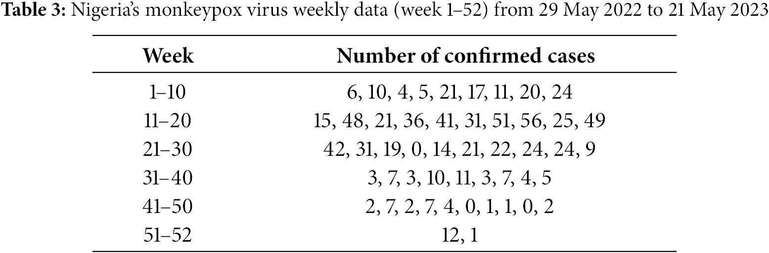

Figure 2: Real data with ABC fractional method
10 CPU Time
The implementation of fractional models (where ζ is less than one) consumes additional CPU(Python) resources because of their memory effects alongside generating superior epidemic results as shown in Fig. 3. Integer-order models that use ζ=1 perform calculations at a superior level that allows them to decrease CPU time by more than 50% in large-scale real-time simulation applications. The computational times between Caputo and ABC exhibit equivalence, thus enabling users to select based on prediction accuracy needs.

Figure 3: CPU time on fractional Caputo and ABC methods
Existence and uniqueness of solutions of the 𝒜ℬ𝒞 fractional derivative model
In this section, we prove the existence and uniqueness of the solution for model (1) by applying the integral operator as defined in Atangana and Baleanu [22] which yields
{L˘(j)=L˘(0)+J˘jζ0 𝒜ℬ𝒞(Λ−νL˘−(ϵ1+ϱ)L˘),Q˘(j)=Q˘(0)+J˘jζ0 𝒜ℬ𝒞(νL˘−(ϱ+ ϑ)Q˘),T˘(j)=T˘(0)+J˘jζ0 𝒜ℬ𝒞(ϑ(1−p)Q˘−(ϱ+ ς)T˘),H˘(j)=H˘(0)+J˘jζ0 𝒜ℬ𝒞(ς(1 −ϵ2)T˘ + ϑpQ˘−(ϱ+ ω+χ+τ)H˘),E˘(j)=E˘(0)+J˘jζ0 𝒜ℬ𝒞(χH˘−(ϱ+ ω+℘)E˘),F˘(j)=F˘(0)+J˘jζ0 𝒜ℬ𝒞(ςϵ2T˘ +ϵ1L˘ +τH˘+℘E˘ −ϱF˘).(35)
Using the same notation as in [22], Eq. (35) becomes
{L˘(j)=L˘(0)+1−ζℳ(ζ)(Λ−νL˘−(ϵ1+ϱ)L˘),+ζℳ(ζ)℘(ζ)∫0j(j−ξ)ζ−1(Λ−νL˘−(ϵ1+ϱ)L˘)dξ,Q˘(j)=Q˘(0)+1−ζℳ(ζ)(νL˘−(ϱ+ ϑ)Q˘),+ζℳ(ζ)℘(ζ)∫0j(j−ξ)ζ−1(νL˘−(ϱ+ ϑ)Q˘)dξ,T˘(j)=T˘(0)+1−ζℳ(ζ)(ϑ(1−p)Q˘−(ϱ+ ς)T˘),+ζℳ(ζ)℘(ζ)∫0j(j−ξ)ζ−1(ϑ(1−p)Q˘−(ϱ+ ς)T˘)dξH˘(j)=H˘(0)+1−ζℳ(ζ)(ς(1 −ϵ2)T˘ + ϑpQ˘−(ϱ+ ω+χ+τ)H˘),+ζℳ(ζ)℘(ζ)∫0j(j−ξ)ζ−1(ς(1 −ϵ2)T˘ + ϑpQ˘−(ϱ+ ω+χ+τ)H˘)dξ,E˘(j)=E˘(0)+1−ζℳ(ζ)(χH˘−(ϱ+ ω+℘)E˘)+ζℳ(ζ)℘(ζ)∫0j(j−ξ)ζ−1(χH˘−(ϱ+ ω+℘)E˘)dξ,F˘(j)=F˘(0)+1−ζℳ(ζ)(ςϵ2T˘ +ϵ1L˘ +τH˘+℘E˘ −ϱF˘)+ζℳ(ζ)℘(ζ)∫0j(j−ξ)ζ−1(ςϵ2T˘ +ϵ1L˘ +τH˘+℘E˘ −ϱF˘)dξ.(36)
Without loss of generality and for simplification of notations, we shall denote
{Ψ1(j,L˘)=Λ−νL˘−(ϵ1+ϱ)L˘,Ψ2(j,Q˘)=νL˘−(ϱ+ ϑ)Q˘,Ψ3(j,T˘)=ϑ(1−p)Q˘−(ϱ+ ς)T˘,Ψ4(j,H˘)=ς(1 −ϵ2)T˘ + ϑpQ˘−(ϱ+ ω+χ+τ)H˘,Ψ5(j,E˘)=χH˘−(ϱ+ ω+℘)E˘,Ψ6(j,F˘)=ςϵ2T˘ +ϵ1L˘ +τH˘+℘E˘ −ϱF˘.(37)
(𝒢:) For proving our results, we consider the following assumption: For this, L˘(j),L˘⋆(j),Q˘(j),Q˘⋆(j),T˘(j),T˘⋆(j),H˘(j),H˘⋆(j),E˘(j),E˘⋆(j),F˘(j),F˘⋆(j)∈ℒ[0,1] be continuous such that ||L˘(j)||≤c1, ||Q˘(j)||≤c2, ||T˘(j)||≤c3, ||H˘(j)||≤c4, ||E˘(j)||≤c5 and ||F˘(j)||≤c6, for some positive constants c1,c2,c3,c4,c5,c6>0.
Theorem 8: Each kernel (Ψ1,Ψ2,Ψ3,Ψ4,Ψ5,Ψ6) satisfy the Lipschitz condition and contraction under the assumption (𝒢) and
cb<1,forb=1,2,3,4,5,6.
Proof: Now,
||Ψ1(j,L˘)−Ψ1(j,L˘1)||=||(L˘−L˘1)(ν)+(L˘−L˘1)(ϵ1+ϱ))||≤ν||L˘−L˘1||+(ϵ1+ϱ)||L˘−L˘1||≤(ν+ϵ1+ϱ)||L˘−L˘1||=c1||L˘−L˘1||,
where c1=ν+ϵ1+ϱ. Hence,
||Ψ1(j,L˘)−Ψ1(j,L˘1)||≤c1||L˘−L˘1||.
Thus, Ψ1 satisfies the Lipschitz condition. Continuing in this manner, we can prove that (Ψ2,Ψ3,Ψ4,Ψ5,Ψ6) satisfy the Lipschitz conditions.
||Ψ2(j,Q˘)−Ψ2(j,Q˘1)||≤c2||Q˘−Q˘1||||Ψ3(j,T˘)−Ψ3(j,T˘1)||≤c3||T˘−T˘1||||Ψ4(j,H˘)−Ψ4(j,H˘1)||≤c4||H˘−H˘1||||Ψ5(j,E˘)−Ψ5(j,E˘1)||≤c4||E˘ −E˘1||||Ψ6(j,F˘)−Ψ6(j,F˘1)||≤c5||F˘−F˘1||.
□
Now, from (36), we have
{L˘(j)=L˘(0)+1−ζℳ(ζ)Ψ1(j,L˘)+ζℳ(ζ)℘(ζ)∫0j(j−ξ)ζ−1Ψ1(ξ,L˘)dξ,Q˘(j)=Q˘(0)+1−ζℳ(ζ)Ψ2(j,Q˘)+ζℳ(ζ)℘(ζ)∫0j(j−ξ)ζ−1Ψ2(ξ,Q˘)dξ,T˘(j)=T˘(0)+1−ζℳ(ζ)Ψ3(j,T˘)+ζℳ(ζ)℘(ζ)∫0j(j−ξ)ζ−1Ψ3(ξ,T˘)dξ,H˘(j)=H˘(0)+1−ζℳ(ζ)Ψ4(j,H˘)+ζℳ(ζ)℘(ζ)∫0j(j−ξ)ζ−1Ψ4(ξ,H˘)dξ,E˘(j)=E˘(0)+1−ζℳ(ζ)Ψ5(j,E˘)+ζℳ(ζ)℘(ζ)∫0j(j−ξ)ζ−1Ψ5(ξ,E˘)dξ,F˘(j)=F˘(0)+1−ζℳ(ζ)Ψ6(j,F˘)+ζℳ(ζ)℘(ζ)∫0j(j−ξ)ζ−1Ψ6(ξ,F˘)dξ,
with the initial conditions
L˘(0)=L˘0,Q˘(0)=𝒱0,T˘(0)=Q˘0,H˘(0)=H˘0,E˘(0)=E˘0,F˘(0)=F˘0.
Suppose, we define the iterative recursive forms below,
{L˘v(j)=L˘(0)+1−ζℳ(ζ)Ψ1(j,L˘v−1)+ζℳ(ζ)℘(ζ)∫0j(j−ξ)ζ−1Ψ1(ξ,L˘v−1)dξ,Q˘v(j)=Q˘(0)+1−ζℳ(ζ)Ψ2(j,Q˘v−1)+ζℳ(ζ)℘(ζ)∫0j(j−ξ)ζ−1Ψ2(ξ,Q˘v−1)dξ,T˘v(j)=T˘(0)+1−ζℳ(ζ)Ψ3(j,T˘v−1)+ζℳ(ζ)℘(ζ)∫0j(j−ξ)ζ−1Ψ3(ξ,T˘v−1)dξ,H˘v(j)=H˘(0)+1−ζℳ(ζ)Ψ4(j,H˘v−1)+ζℳ(ζ)℘(ζ)∫0j(j−ξ)ζ−1Ψ4(ξ,H˘v−1)dξE˘v(j)=E˘(0)+1−ζℳ(ζ)Ψ5(j,E˘v−1)+ζℳ(ζ)℘(ζ)∫0j(j−ξ)ζ−1Ψ5(ξ,E˘v−1)dξF˘v(j)=F˘(0)+1−ζℳ(ζ)Ψ6(j,F˘v−1)+ζℳ(ζ)℘(ζ)∫0j(j−ξ)ζ−1Ψ6(ξ,F˘v−1)dξ.
with the initial conditions
L˘(0)=L˘0,Q˘(0)=Q˘0,T˘(0)=T˘0,H˘(0)=H˘0,E˘(0)=E˘0,F˘(0)=F˘0.
The following system of equations is formed by using the initial conditions and the difference between the succeeding terms.
ωv(j)=L˘v(j)−L˘v−1(j)=1−ζℳ(ζ)(Ψ1(j,L˘v−1)−Ψ1(j,L˘v−2))+ζℳ(ζ)℘(ζ)∫0j(j−ξ)ζ−1(Ψ1(j,L˘v−1)−Ψ1(j,L˘v−2))dξ,ℵv(j)=Q˘v(j)−Q˘v−1(j)=1−ζℳ(ζ)(Ψ2(j,Q˘v−1)−Ψ2(j,Q˘v−2))+ζℳ(ζ)℘(ζ)∫0j(j−ξ)ζ−1(Ψ2(j,Q˘v−1)−Ψ2(j,Q˘v−2))dξ,Υv(j)=T˘v(j)−T˘v−1(j)=1−ζℳ(ζ)(Ψ3(j,T˘v−1)−Ψ3(j,T˘v−2))+ζℳ(ζ)℘(ζ)∫0j(j−ξ)ζ−1(Ψ3(j,T˘v−1)−Ψ3(j,T˘v−2))dξ,Ξv(j)=H˘v(j)−H˘v−1(j)=1−ζℳ(ζ)(Ψ4(j,H˘v−1)−Ψ4(j,H˘v−2))+ζℳ(ζ)℘(ζ)∫0j(j−ξ)ζ−1(Ψ4(j,H˘v−1)−Ψ4(j,H˘v−2))dξ,Θv(j)=E˘v(j)−E˘v−1(j)=1−ζℳ(ζ)(Ψ5(j,E˘v−1)−Ψ5(j,E˘v−2))+ζℳ(ζ)℘(ζ)∫0j(j−ξ)ζ−1(Ψ5(j,E˘v−1)−Ψ5(j,E˘v−2))dξ,ℱv(j)=F˘v(j)−F˘v−1(j)=1−ζℳ(ζ)(Ψ6(j,F˘v−1)−Ψ6(j,F˘v−2))+ζℳ(ζ)℘(ζ)∫0j(j−ξ)ζ−1(Ψ6(j,F˘v−1)−Ψ6(j,F˘v−2))dξ.(38)
It should be noted that
L˘v(j)=∑r=1ζωr(j),Q˘v(j)=∑r=1ζℵr(j),T˘v(j)=∑r=1ζΥr(j),H˘v(j)=∑r=1ζΞr(j),E˘v(j)=∑r=1ζΘr(j),F˘v(j)=∑r=1ζℱr(j).(39)
By taking (38), the triangular inequality is taken into account. After applying the norm to (39).
||ωv(j)||=||L˘v(j)−L˘v−1(j)||=1−ζℳ(ζ)||Ψ1(j,L˘v−1)−Ψ1(j,L˘v−2)||+ζℳ(ζ)℘(ζ)‖∫0j(j−ξ)ζ−1(Ψ1(j,L˘v−1)−Ψ1(j,L˘v−2))dξ‖.(40)
As the Lipschitz condition is satisfied by the kernel, the following equation is obtained
||L˘v(j)−L˘v−1(j)||≤1−ζℳ(ζ)||L˘v−1−L˘v−2||+ζℳ(ζ)℘(ζ)∫0j(j−ξ)ζ−1||L˘v−1−L˘v−2||dξ,
also,
||ωv(j)||≤1−ζℳ(ζ)c1||ωv−1(j)||+ζℳ(ζ)℘(ζ)c1∫0j(j−ξ)ζ−1||ωv−1(ξ)||dξ.(41)
In the same manner, we get
||ℵv(j)||≤1−ζℳ(ζ)c2||ℵv−1(j)||+ζℳ(ζ)℘(ζ)c2∫0j(j−ξ)ζ−1||ℵv−1(ξ)||dξ,||Υv(j)||≤1−ζℳ(ζ)c3||Υv−1(j)||+ζℳ(ζ)℘(ζ)c3∫0j(j−ξ)ζ−1||Υv−1(ξ)||dξ,||Ξv(j)||≤1−ζℳ(ζ)c4||Ξv−1(j)||+ζℳ(ζ)℘(ζ)c4∫0j(j−ξ)ζ−1||Ξv−1(ξ)||dξ,||Θv(j)||≤1−ζℳ(ζ)c5||Θv−1(j)||+ζℳ(ζ)℘(ζ)c5∫0j(j−ξ)ζ−1||Θv−1(ξ)||dξ,||ℱv(j)||≤1−ζℳ(ζ)c6||ℱv−1(j)||+ζℳ(ζ)℘(ζ)c6∫0j(j−ξ)ζ−1||ℱv−1(ξ)||dξ.
Theorem 9: The Monkeypox virus disease model with 𝒜ℬ𝒞 fractional derivative (1) has a unique solution if for jmax the following condition satisfied
(1−ζℳ(ζ)+jmaxζζℳ(ζ)℘(ζ))cb≤1,forb=1,2,3,4,5,6.
Proof: It is clear that L˘(j), Q˘(j), T˘(j), H˘(j), E˘(j) and F˘(j) are bounded. The kernels of these functions also satisfy the Lipschitz condition. Therefore, employing the succeeding relation with the application of the (41), we get
||ωv(j)||≤||L˘(0)||(1−ζℳ(ζ)c1+bζζℳ(ζ)℘(ζ)c1)ζ||ℵv(j)||≤||Q˘(0)||(1−ζℳ(ζ)c2+bζζℳ(ζ)℘(ζ)c2)ζ||Υv(j)||≤||T˘(0)||(1−ζℳ(ζ)c3+bζζℳ(ζ)℘(ζ)c3)ζ||Ξv(j)||≤||H˘(0)||(1−ζℳ(ζ)c4bζζℳ(ζ)℘(ζ)c4)ζ||Θv(j)||≤||E˘(0)||(1−ζℳ(ζ)c5bζζℳ(ζ)℘(ζ)c5)ζ||ℱv(j)||≤||F˘(0)||(1−ζℳ(ζ)c6+bζζℳ(ζ)℘(ζ)c6)ζ.
Hence, (39) is a smooth function and exists. Let us suppose that the aforementioned functions represent the model’s solutions.
L˘(j)−L˘(0)=L˘ζ(j)−Θ1(ζ)(j),Q˘(j)−Q˘(0)=Q˘ζ(j)−Θ2(ζ)(j),T˘(j)−T˘(0)=T˘ζ(j)−Θ3(ζ)(j),H˘(j)−H˘(0)=H˘ζ(j)−Θ4(ζ)(j),E˘(j)−E˘(0)=E˘ζ(j)−Θ5(ζ)(j),F˘(j)−F˘(0)=F˘ζ(j)−Θ6(ζ)(j).
The term ||Θ∞(j)||→0 at infinity. For this,
||Θ1(ζ)(j)||≤‖1−ζℳ(ζ)(Ψ1(j,L˘)−Ψ1(j,L˘v−1))+ζℳ(ζ)℘(ζ)∫0j(j−ξ)ζ−1(Ψ1(j,L˘)−Ψ1(j,L˘v−1))dξ‖≤1−ζℳ(ζ)||Ψ1(j,L˘)−Ψ1(j,L˘v−1)||+ζℳ(ζ)℘(ζ)∫0j(j−ξ)ζ−1||Ψ1(j,L˘)−Ψ1(j,L˘v−1)||dξ≤1−ζℳ(ζ)c1||L˘−L˘ζ−1||+ζjζℳ(ζ)℘(ζ)c1||L˘−L˘ζ−1||.
By recursively repeating the process, we get
||Θ1(ζ)(j)||≤(1−ζℳ(ζ)+ζjζℳ(ζ)℘(ζ))ζ+1c1ζ𝒴.
Then, for jmax, we get
||Θ1(ζ)(j)||≤(1−ζℳ(ζ)+ζjmaxζℳ(ζ)℘(ζ))ζ+1c1ζ𝒴.
By taking the limit on both sides as ζ→∞, we get ||Θ∞(j)||→0. To prove uniqueness of the solution. For this, assume that there exists another solution L˘⋆(j), Q˘⋆(j), T˘⋆(j), H˘⋆(j), E˘⋆(j), F˘⋆(j) with initial values such that
L˘⋆(j)=L˘(0)+1−ζℳ(ζ)Ψ1(j,L˘⋆)+ζℳ(ζ)℘(ζ)∫0j(j−ξ)ζ−1Ψ1(ξ,L˘⋆)dξ,Q˘⋆(j)=Q˘(0)+1−ζℳ(ζ)Ψ2(j,Q˘⋆)+ζℳ(ζ)℘(ζ)∫0j(j−ξ)ζ−1Ψ2(ξ,Q˘⋆)dξ,T˘⋆(j)=Q˘(0)+1−ζℳ(ζ)Ψ3(j,T˘⋆)+ζℳ(ζ)℘(ζ)∫0j(j−ξ)ζ−1Ψ3(ξ,T˘⋆)dξ,H˘⋆(j)=H˘(0)+1−ζℳ(ζ)Ψ4(j,H˘⋆)+ζℳ(ζ)℘(ζ)∫0j(j−ξ)ζ−1Ψ4(ξ,H˘⋆)dξ,E˘⋆(j)=H˘(0)+1−ζℳ(ζ)Ψ5(j,E˘⋆)+ζℳ(ζ)℘(ζ)∫0j(j−ξ)ζ−1Ψ5(ξ,E˘⋆)dξ,F˘⋆(j)=F˘(0)+1−ζℳ(ζ)Ψ6(j,F˘⋆)+ζℳ(ζ)℘(ζ)∫0j(j−ξ)ζ−1Ψ6(ξ,F˘⋆)dξ.
Now,
||L˘−L˘⋆||=‖1−ζℳ(ζ)(Ψ1(j,L˘)−Ψ1(j,L˘⋆))+ζℳ(ζ)℘(ζ)∫0j(j−ξ)ζ−1(Ψ1(ξ,L˘)−Ψ1(ξ,L˘⋆))dξ‖≤1−ζℳ(ζ)‖Ψ1(j,L˘)−Ψ1(j,L˘⋆)‖+ζℳ(ζ)℘(ζ)∫0j(j−ξ)ζ−1‖Ψ1(ξ,L˘)−Ψ1(ξ,L˘⋆))‖dξ≤1−ζℳ(ζ)c1||L˘−L˘⋆||+ζℳ(ζ)℘(ζ)∫0jc1(j−ξ)ζ−1||L˘−L˘⋆||dξ=1−ζℳ(ζ)c1||L˘−L˘⋆||+ζℳ(ζ)℘(ζ)c1∫0j(j−ξ)ζ−1||L˘−L˘⋆||dξ≤(1−ζℳ(ζ)+ζjζℳ(ζ)℘(ζ))c1||L˘−L˘⋆||≤(1−ζℳ(ζ)+ζjζℳ(ζ)℘(ζ))c1||L˘−L˘⋆||,
which implies that
(1−(1−ζℳ(ζ)+ζjζℳ(ζ)℘(ζ))c1)||L˘−L˘⋆||≤0.
Therefore, ||L˘−L˘⋆||=0. Hence, L˘=L˘⋆. Similarly, we can prove
Q˘=Q˘⋆,T˘=T˘⋆,H˘=H˘⋆,E˘=E˘⋆,F˘=F˘⋆.
Hence, Monkeypox virus disease model with 𝒜ℬ𝒞 fractional derivative (1) has a unique solution. □
11 Ulam Hyers and Ulam Hyers Rassias Stability of the Monkeypox Virus Disease Model
In this section, we obtain the Ulam Hyers and Ulam Hyers Rassias stability of the Monkeypox virus disease model with 𝒜ℬ𝒞 fractional derivative (1). We state the required definition.
Definition 8: The Monkeypox virus disease model with 𝒜ℬ𝒞 fractional derivative (1) has Ulam Hyers stability if there exist constants Ψb>0, b=1,2,3,4,5,6 satisfying: For every ϵb>0, b=1,2,3,4,5,6, if
{|0𝒜ℬ𝒞𝒟jζL˘(j)−Ψ1(j,L˘)|≤ϵ1,|0𝒜ℬ𝒞𝒟jζQ˘(j)−Ψ2(j,Q˘)|≤ϵ2,|0𝒜ℬ𝒞𝒟jζT˘(j)−Ψ3(j,T˘)|≤ϵ3,|0𝒜ℬ𝒞𝒟jζH˘(j)−Ψ4(j,H˘)|≤ϵ4,|0𝒜ℬ𝒞𝒟jζE˘(j)−Ψ4(j,E˘)|≤ϵ5,|0𝒜ℬ𝒞𝒟jζF˘(j)−Ψ5(j,F˘)|≤ϵ6,(42)
and there exists a solution of the Monkeypox virus disease model with 𝒜ℬ𝒞 fractional derivative (1), L˘⋆(j),Q˘⋆(j),T˘⋆(j),H˘⋆(j), E˘⋆(j) and F˘⋆(j) that statisfying the given model, such that
||L˘−L˘⋆||≤η1ϵ1,||Q˘−Q˘⋆||≤η2ϵ2,||T˘−T˘⋆||≤η3ϵ3,||H˘−H˘⋆||≤η4ϵ4,||E˘ −E˘⋆||≤η5ϵ5,||F˘−F˘⋆||≤η6ϵ6
Remark 2: Consider that function L˘ is a solution of the first inequality (42) iff a continuous function h1 exists (depending on L˘1) so that
(A1) |h1(j)|<ϵ1, and
(A2) 𝒟jζ0 𝒜ℬ𝒞L˘(j)=Ψ1(j,L˘)+h1(j).
Similarly, we can define for other classes of the model (42) for some hb where b=2,3,4,5,6.
Theorem 10: Assume that the hypothesis (𝒢) holds true. Then the Monkeypox virus disease model with 𝒜ℬ𝒞 (1) is Ulam Hyers stable if
(1−ζℳ(ζ)+jζζℳ(ζ)℘(ζ))cb≤1,forb=1,2,3,4,5,6.
Proof: Let ϵ1>0 and the function L˘ be arbitary such that
|𝒟jζ0 𝒜ℬ𝒞L˘(j)−Ψ1(j,L˘)|≤ϵ1.
According to Remark 2, we have a function h1 with |h1|<ϵ1, which satisfies
𝒟jζ0 𝒜ℬ𝒞L˘(j)=Ψ1(j,L˘)+h1(j).
Accordingly, we get
L˘(j)=L˘(0)+1−ζℳ(ζ)Ψ1(j,L˘)+ζℳ(ζ)℘(ζ)∫0j(j−ξ)ζ−1Ψ1(ξ,L˘)dξ+1−ζℳ(ζ)h1(j)+ζℳ(ζ)℘(ζ)∫0j(j−ξ)ζ−1h1(ξ)dξ.
Let L˘⋆ be the unique solution of the Monkeypox virus disease model with 𝒜ℬ𝒞 fractional derivative (1). Then,
L˘⋆(j)=L˘(0)+1−ζℳ(ζ)Ψ1(j,L˘⋆)+ζℳ(ζ)℘(ζ)∫0j(j−ξ)ζ−1Ψ1(ξ,L˘⋆)dξ.
Hence,
|L˘(j)−L˘⋆(j)|≤1−ζℳ(ζ)|Ψ1(j,L˘(j))−Ψ1(j,L˘⋆(j))|+ζℳ(ζ)℘(ζ)∫0j(j−ξ)ζ−1|Ψ1(ξ,L˘(j))−Ψ1(ξ,L˘⋆(j))|dξ+1−ζℳ(ζ)|h1(j)|+ζℳ(ζ)℘(ζ)∫0j(j−ξ)ζ−1|h1(ξ)|dξ≤[1−ζℳ(ζ)+ζjζℳ(ζ)℘(ζ)]c1|L˘(j)−L˘⋆(j)|+[1−ζℳ(ζ)+ζjζℳ(ζ)℘(ζ)]ϵ1||L˘(j)−L˘⋆(j)||≤[1−ζℳ(ζ)+ζjζℳ(ζ)℘(ζ)]ϵ11−[1−ζℳ(ζ)+ζjζℳ(ζ)℘(ζ)]c1.
Then,
||L˘(j)−L˘⋆(j)||≤η1ϵ1,
where
η1=[1−ζℳ(ζ)+ζjζℳ(ζ)℘(ζ)]1−[1−ζℳ(ζ)+ζjζℳ(ζ)℘(ζ)]c1.
Similarly, we have
||Q˘−Q˘⋆||≤η2ϵ2,||T˘−T˘⋆||≤η3ϵ3,||H˘−H˘⋆||≤η4ϵ4,||E˘ −E˘⋆||≤η5ϵ5,||F˘−F˘⋆||≤η6ϵ6.
Thus, Monkeypox virus disease model with 𝒜ℬ𝒞 fractional derivative (1) is Ulam Hyers stable. □
Definition 9: The Monkeypox virus disease model with 𝒜ℬ𝒞 fractional derivative (1) has Ulam Hyers Rassias stability if there exist constants Ψb>0 and a function yb(t)∈𝒞([0,1]→R), b=1,2,3,4,5,6 satisfying: For every ϵb>0b=1,2,3,4,5,6, if
{|0𝒜ℬ𝒞𝒟jζL˘(j)−Ψ1(j,L˘)|≤ ϵ1y1(t),|0𝒜ℬ𝒞𝒟jζQ˘(j)−Ψ2(j,Q˘)|≤ ϵ2y2(t),|0𝒜ℬ𝒞𝒟jζT˘(j)−Ψ3(j,T˘)|≤ ϵ3y3(t),|0𝒜ℬ𝒞𝒟jζH˘(j)−Ψ4(j,H˘)|≤ ϵ4y4(t),|0𝒜ℬ𝒞𝒟jζE˘(j)−Ψ4(j,E˘)|≤ ϵ5y5(t),|0𝒜ℬ𝒞𝒟jζF˘(j)−Ψ5(j,F˘)|≤ ϵ6y6(t),(43)
and there exists a solution of the Monkeypox virus disease model with 𝒜ℬ𝒞 fractional derivative (1), L˘⋆(j),Q˘⋆(j),T˘⋆(j),H˘⋆(j), E˘⋆(j) and F˘⋆(j) that statisfying the given model, such that
||L˘−L˘⋆||≤η1ϵ1y1(t),||Q˘−Q˘⋆||≤η2ϵ2y2(t),||T˘−T˘⋆||≤η3ϵ3y3(t),||H˘−H˘⋆||≤η4ϵ4y4(t),||E˘ −E˘⋆||≤η5ϵ5y5(t),||F˘−F˘⋆||≤η6ϵ6y6(t).
Remark 3: Consider that function L˘ is a solution of the first inequality (43) iff a continuous function h1 exists (depending on L˘1) so that
(B1) |h1(j)|<ϵ1y1(t), and
(B2) 𝒟jζ0 𝒜ℬ𝒞L˘(j)=Ψ1(j,L˘)+h1(j).
Similarly, we can define for other classes of the model (43) for some hb where b=2,3,4,5,6.
Theorem 11: Assume that the hypothesis (𝒢) holds true. Then the Monkeypox virus disease model with 𝒜ℬ𝒞 (1) is Ulam Hyers Rassias stable if
(1−ζℳ(ζ)+jζζℳ(ζ)℘(ζ))cb≤1,forb=1,2,3,4,5,6.
Proof: Let ϵ1>0 and the function L˘ be arbitary such that
|0𝒜ℬ𝒞𝒟jζL˘(j)−Ψ1(j,L˘)|≤ϵ1y1(t).
According to Remark 2, we have a function h1 with |h1|<ϵ1y1(t), which satisfies
𝒟jζ0 𝒜ℬ𝒞L˘(j)=Ψ1(j,L˘)+h1(j).
Accordingly, we get
L˘(j)=L˘(0)+1−ζℳ(ζ)Ψ1(j,L˘)+ζℳ(ζ)℘(ζ)∫0j(j−ξ)ζ−1Ψ1(ξ,L˘)dξ+1−ζℳ(ζ)h1(j)+ζℳ(ζ)℘(ζ)∫0j(j−ξ)ζ−1h1(ξ)dξ
Let L˘⋆ be the unique solution of the Monkeypox virus disease model with 𝒜ℬ𝒞 fractional derivative (1). Then,
L˘⋆(j)=L˘(0)+1−ζℳ(ζ)Ψ1(j,L˘⋆)+ζℳ(ζ)℘(ζ)∫0j(j−ξ)ζ−1Ψ1(ξ,L˘⋆)dξ.
Hence,
|L˘(j)−L˘⋆(j)|≤1−ζℳ(ζ)|Ψ1(j,L˘(j))−Ψ1(j,L˘⋆(j))|+ζℳ(ζ)℘(ζ)∫0j(j−ξ)ζ−1|Ψ1(ξ,L˘(j))−Ψ1(ξ,L˘⋆(j))|dξ+1−ζℳ(ζ)|h1(j)|+ζℳ(ζ)℘(ζ)∫0j(j−ξ)ζ−1|h1(ξ)|dξ≤[1−ζℳ(ζ)+ζjζℳ(ζ)℘(ζ)]c1|L˘(j)−L˘⋆(j)|+[1−ζℳ(ζ)+ζjζℳ(ζ)℘(ζ)]ϵ1y1(t)||L˘(j)−L˘⋆(j)||≤[1−ζℳ(ζ)+ζjζℳ(ζ)℘(ζ)]ϵ1y1(t)1−[1−ζℳ(ζ)+ζjζℳ(ζ)℘(ζ)]c1.
Then,
||L˘(j)−L˘⋆(j)||≤η1ϵ1y1(t),
where
η1=[1−ζℳ(ζ)+ζjζℳ(ζ)℘(ζ)]1−[1−ζℳ(ζ)+ζjζℳ(ζ)℘(ζ)]c1.
Similarly, we have
||Q˘−Q˘⋆||≤η2ϵ2y2(t),||T˘−T˘⋆||≤η3ϵ3y3(t),||H˘−H˘⋆||≤η4ϵ4y4(t),||E˘ −E˘⋆||≤η5ϵ5y5(t),||F˘−F˘⋆||≤η6ϵ6y1(t).
Thus, Monkeypox virus disease model with 𝒜ℬ𝒞 fractional derivative (1) is Ulam Hyers Rassias stable. □
12 Numerical Scheme on 𝒜ℬ𝒞 Operator
Here, a numerical scheme for the Monkeypox virus disease model with 𝒜ℬ𝒞 fractional derivative (1) is developed. For this, we use the approach related to Langrange interpolation polynomials. Consider a general Cauchy problem with fractal fractional differential operator as
{𝒟jζ0 𝒜ℬ𝒞χ(j)=Ψ(j,χ(j))χ(0)=χ0.(44)
Utilizing the fractal fractional integral operator, we obtain
χ(j)=χ(0)+1−ζℳ(ζ)Ψ(j,χ(j))+ζℳ(ζ)℘(ζ)∫0j(j−ξ)ζ−1Ψ(ξ,χ(ξ))dξ.
Putting j by ji+1, which gives
χi+1=χ(0)+1−ζℳ(ζ)Ψ(ji,χ(ji))+ζℳ(ζ)℘(ζ)∫0ji+1(ji+1−ξ)ζ−1Ψ(ξ,χ(ξ))dξ.(45)
Over the closed interval [jm,jm+1], the function Ψ(ξ,χ(ξ)) can be approximated by the interpolation polynomial
θm(ξ)=Ψ(jm,χ(jm))h(ξ−jm−1)−Ψ(jm−1,χ(ξm−1))h(ξ−jm),≅Ψ(jm,χm)h(ξ−jm−1)−Ψ(jm−1,χm−1)h(ξ−jm),
where h=jm−jm−1. By assuming (45) again for Ψ(ξ,χ(ξ)) and Langrange interpolation where h is step length, one gets
χi+1=χ(0)+1−ζℳ(ζ)Ψ(ji,χ(ji))+ζℳ(ζ)℘(ζ)∑c=0i(Ψ(jc,χc)h∫jcjc+1(ξ−jc−1)(ji+1−ξ)ζ−1dξ−Ψ(jc−1,χc−1)h∫jcjc+1(ξ−jc)(ji+1−ξ)ζ−1dξ).(46)
Now,
∫jcjc+1(ξ−jc−1)(ji+1−ξ)ζ−1dξ=hζ+1(i−j+1)ζ(i−j+ζ+2)−(i−c)ζ(i−c+2+2ζ)ζ(ζ+1),
and
∫jcjc+1(ξ−jc)(ji+1−ξ)ζ−1dξ=hζ+1(i−j+1)ζ+1−(i−c)ζ(i+1−c+ζ)ζ(ζ+1)
Consequently,
χi+1=χ(0)+1−ζℳ(ζ)Ψ(ji,χi)+ζℳ(ζ)∑c=0i(Ψ(jc,χc)℘(ζ+2)hζ((i−j+1)ζ(i−j+ζ+2)−(i−c)ζ(i−c+2+2ζ)))−ζℳ(ζ)∑c=0i(Ψ(jc−1,χc−1)℘(ζ+2)hζ((i−j+1)ζ+1−(i−c)ζ(i+1−c+ζ))).(47)
Hence, the numerical scheme for (36) is obtained as the following:
L˘i+1=L˘(0)+1−ζℳ(ζ)Ψ1(ji,L˘i)+ζℳ(ζ)∑c=0i(Ψ1(jc,L˘c)℘(ζ+2)hζ((i−j+1)ζ(i−j+ζ+2)−(i−c)ζ(i−c+2+2ζ)))−ζℳ(ζ)∑c=0i(Ψ1(jc−1,L˘c−1)℘(ζ+2)hζ((i−j+1)ζ+1−(i−c)ζ(i+1−c+ζ))),
Q˘i+1=Q˘(0)+1−ζℳ(ζ)Ψ2(ji,𝒱i)+ζℳ(ζ)∑c=0i(Ψ2(jc,Q˘c)℘(ζ+2)hζ((i−j+1)ζ(i−j+ζ+2)−(i−c)ζ(i−c+2+2ζ)))−ζℳ(ζ)∑c=0i(Ψ2(jc−1,Q˘c−1)℘(ζ+2)hζ((i−j+1)ζ+1−(i−c)ζ(i+1−c+ζ))),
T˘i+1=T˘(0)+1−ζℳ(ζ)Ψ3(ji,T˘i)+ζℳ(ζ)∑c=0i(Ψ3(jc,T˘c)℘(ζ+2)hζ((i−j+1)ζ(i−j+ζ+2)−(i−c)ζ(i−c+2+2ζ)))−ζℳ(ζ)∑c=0i(Ψ3(jc−1,T˘c−1)℘(ζ+2)hζ((i−j+1)ζ+1−(i−c)ζ(i+1−c+ζ))),
H˘i+1=H˘(0)+1−ζℳ(ζ)Ψ4(ji,H˘i)+ζℳ(ζ)∑c=0i(Ψ4(jc,H˘c)℘(ζ+2)hζ((i−j+1)ζ(i−j+ζ+2)−(i−c)ζ(i−c+2+2ζ)))−ζℳ(ζ)∑c=0i(Ψ4(jc−1,H˘c−1)℘(ζ+2)hζ((i−j+1)ζ+1−(i−c)ζ(i+1−c+ζ))),
E˘i+1=E˘(0)+1−ζℳ(ζ)Ψ5(ji,H˘i)+ζℳ(ζ)∑c=0i(Ψ5(jc,E˘c)℘(ζ+2)hζ((i−j+1)ζ(i−j+ζ+2)−(i−c)ζ(i−c+2+2ζ)))−ζℳ(ζ)∑c=0i(Ψ5(jc−1,E˘c−1)℘(ζ+2)hζ((i−j+1)ζ+1−(i−c)ζ(i+1−c+ζ))),
F˘i+1=F˘(0)+1−ζℳ(ζ)Ψ6(ji,F˘i)+ζℳ(ζ)∑c=0i(Ψ6(jc,F˘c)℘(ζ+2)hζ((i−j+1)ζ(i−j+ζ+2)−(i−c)ζ(i−c+2+2ζ)))−ζℳ(ζ)∑c=0i(Ψ6(jc−1,F˘c−1)℘(ζ+2)hζ((i−j+1)ζ+1−(i−c)ζ(i+1−c+ζ))).
Numerical results and discussion
We deliberated the model of (1) observing Mpox disease. Now we present the numerical outcomes after employment of the parametric values defined in Table 1 that are compatible with Mpox virus diseases for various ζ. Taking initial values as
L˘(0)=73148,Q˘(0)=300,T˘(0)=200,H˘(0)=100,E˘(0)=50,F˘(0)=0.
The numerical simulations for the model (1), incorporating fractional derivatives, provide detailed analyses of the progression of Monkeypox dynamics. Each compartment-Susceptible (L˘), Exposed (Q˘), Asymptomatic (T˘), Infected (H˘), Isolated (E˘), and Recovered (F˘) was examined under varying fractional orders (ζ) to explore the influence of memory effects and fractional dynamics on disease spread and control.
From Fig. 4, we can see that the simulations reveal a rapid decline in the susceptible population for higher fractional orders (ζ = 1.0), indicating accelerated exposure rates and disease progression in deterministic scenarios. Conversely, lower fractional orders (ζ = 0.80) introduce memory effects, slowing the exposure process and extending the susceptible phase. These findings suggest fractional models better capture real-world disease dynamics, where immediate transitions are less common.

Figure 4: Susceptible class
Fig. 5 reveals that the exposed population exhibits an initial rise followed by stabilization. For higher ζ values, the peak occurs earlier, reflecting faster transitions from susceptible to exposed. Lower ζ values delay the peak, showcasing the role of fractional derivatives in extending the incubation phase. These results highlight the importance of timely interventions, such as vaccination or quarantine, to reduce the duration and intensity of exposure.

Figure 5: Exposed class
The asymptomatic compartment demonstrates significant variability under different ζ values and the same is reflected in Fig. 6. Higher fractional orders result in quicker depletion of asymptomatic individuals as they transition to symptomatic or recovery states. In contrast, lower ζ values prolong the presence of asymptomatic carriers, underscoring the need for robust asymptomatic testing and monitoring strategies.

Figure 6: Asymptomatic class
As can be seen in Fig. 7, symptomatic cases peak later under fractional orders closer to ζ = 0.80, reflecting slower disease progression due to memory effects. For ζ values approaching 1.0, symptomatic cases rise sharply and peak earlier, simulating deterministic epidemic curves. These dynamics underline the importance of rapid diagnosis and treatment to mitigate symptomatic burdens, particularly in scenarios with reduced memory effects.

Figure 7: Symptomatic class
Fig. 8 shows that Isolation levels steadily increase across all fractional orders, peaking earlier for higher ζ values. This trend demonstrates the effectiveness of isolation measures in curbing disease transmission in rapid-progression scenarios. Lower fractional orders highlight delayed isolation growth, emphasizing the importance of timely policy interventions.

Figure 8: Isolated class
In Fig. 9 recovery trends exhibit faster growth for higher ζ values, reflecting quicker transitions from symptomatic and isolated states to recovery. In contrast, lower ζ values show delayed recovery, consistent with extended disease progression. These results highlight the role of fractional models in capturing varying recovery timelines and the potential impact of post-exposure treatments or vaccination campaigns.

Figure 9: Recovered class
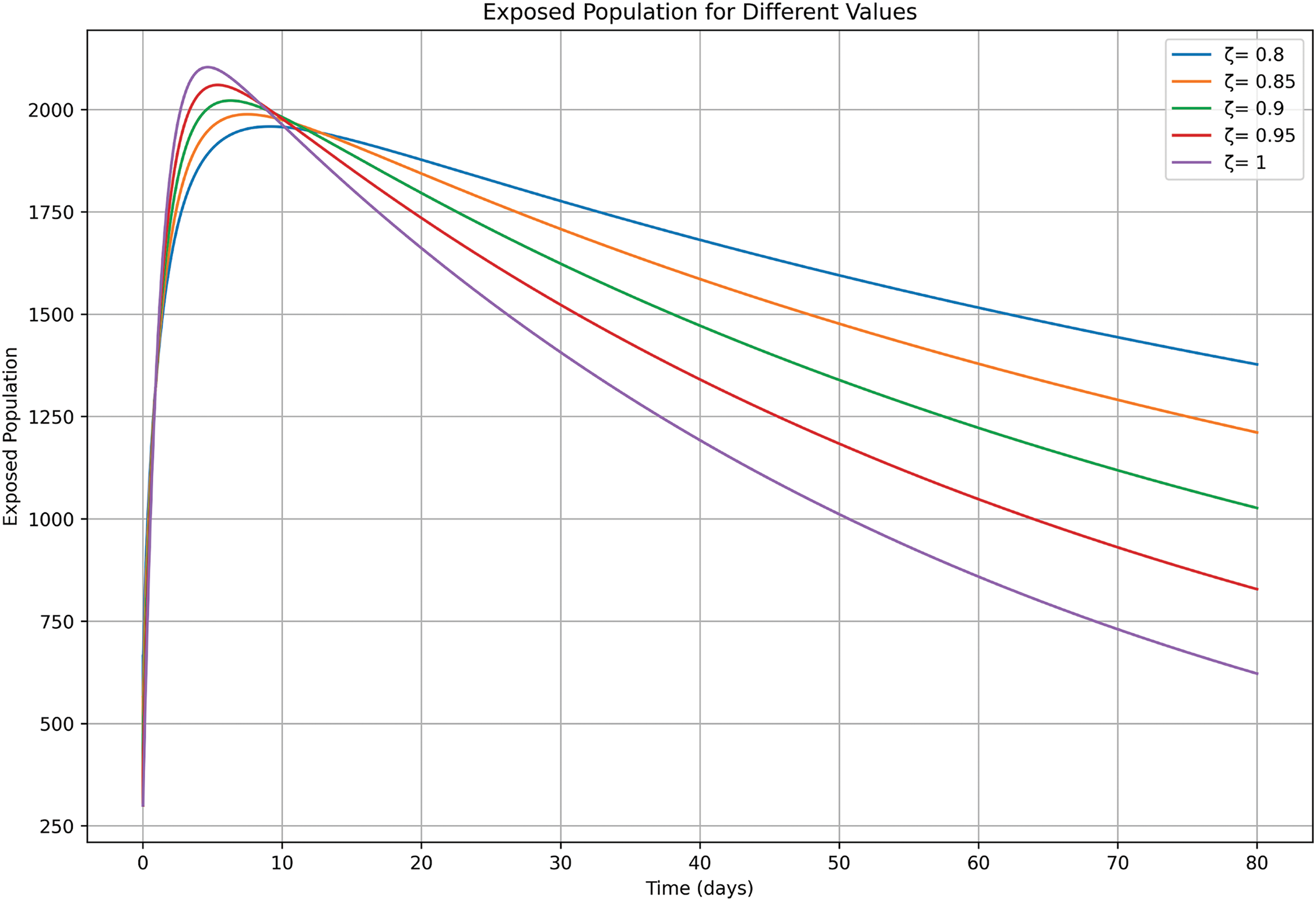
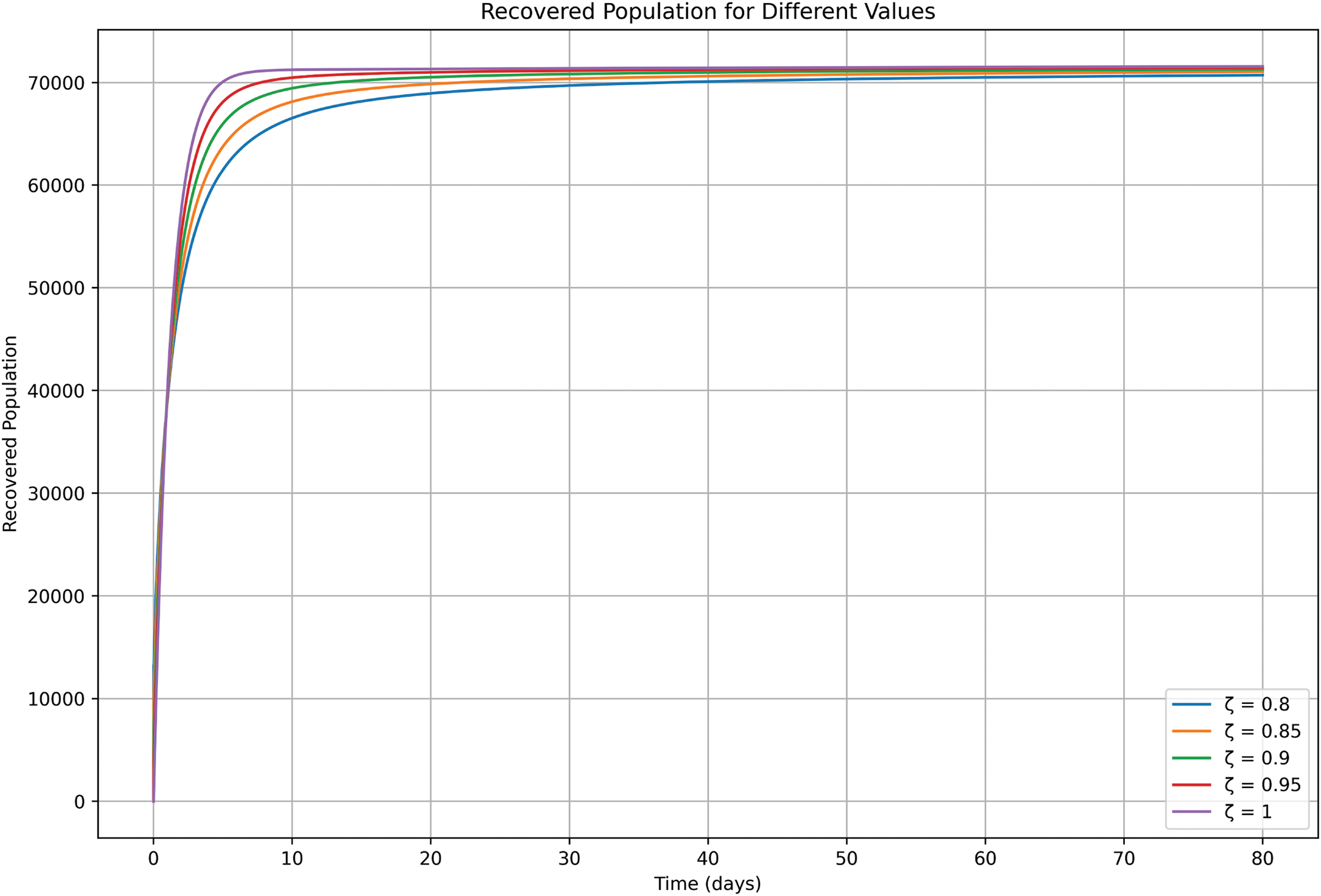
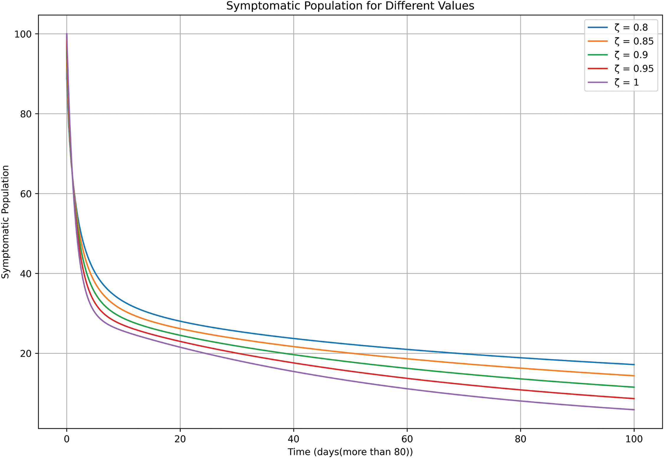
In Fig. 10, susceptible population numbers shift throughout time based on transmission speed levels. Healthcare systems become overwhelmed as the transmission rate ζ increases because the depletion of susceptible individuals happens more rapidly, which leads to rapid disease saturation or herd immunity. A slower transmission rate results in sustainability of the susceptible population during a longer period before interventions take effect. Public health measures should control ζ to determine the epidemic’s speed and limit its effect on healthcare capacity and population health outcomes. The transmission rate ζ directly influences exposed population dynamics according to Fig. 11. Disease spread happens rapidly when ζ is high while the epidemic follows a fast resolution pattern. Lower values of ζ indicate a slower pace of exposed population growth that gives intervention opportunities yet extends epidemic length. Higher transmission rates ζ present in Fig. 12 reduce asymptomatic individual numbers because people swiftly move to symptomatic or isolated stages and deplete this population segment. The epidemic lasts longer because reduced transmission rates slow down the decrease of asymptomatic individuals, allowing additional time for public health responses. The control of the disease becomes more challenging when we lack comprehension of asymptomatic population behavior since these individuals maintain virus transmission despite displaying no symptoms, particularly when transmission rates are low. Fig. 13 symptomatic individuals increase rapidly and intensely in situations with high ζ while the disease progression leads to a quick decrease in cases. The epidemic duration becomes longer when ζ values decrease, while the increase of symptomatic cases occurs more slowly. Successful public health planning requires an understanding of how symptomatic populations behave. A quick epidemic demands emergency responses to protect healthcare capabilities, yet slower epidemics demand long-term, continued interventions after they start. The transmission rate ζ demonstrates substantial influence on both the isolation population development and its duration according to Fig. 14. An epidemic becomes faster and more intense when the value for ζ is higher since isolation needs to be implemented swiftly. A decreased value of ζ allows isolation measures to persist over more time so intervention teams have more opportunities to take action yet the epidemic becomes prolonged. Fig. 15 shows that raising the ζ value results in faster peak achievement of recovered patients. The disease progression along with recovery becomes both speedier when ζ values increase. Conversely, lower A slower disease transmission occurs with ζ values resulting in a systematic increase of the recovered population. Public health interventions need to adapt their disease management techniques according to transmission speed because changing the recovery process affects healthcare capacity and epidemic control measures. The response requires immediate action when transmission rates are high because the disease resolves quickly yet preparedness measures must begin right away. On the other hand, low transmission rates require long-term management to achieve complete recovery.

Figure 10: Susceptible class (j>80)

Figure 11: Exposed class (j>80)

Figure 12: Asymptomatic class (j>80)

Figure 13: Symptomatic class (j>80)

Figure 14: Isolation class (j>80)

Figure 15: Recovered class (j>80)
13 Numerical Scheme on Caputo Operator
We thought about a numerical method which is based upon the Caputo operator that has been discovered to describe the linear and nonlinear dynamical systems [32] and [33]. Now, we assume a fractional order initial value problem using the fractional Caputo operator
{𝒟jζ0𝒞χ(j)=Ψ(j,χ(j))χ(0)=χ0.(48)
Utilizing the fractal fractional integral operator, we obtain
χ(j)=χ(0)+1℘(ζ)∫0j(j−ξ)ζ−1Ψ(ξ,χ(ξ))dξ.
Putting j by ji+1, which gives
χi+1=χ(0)+1℘(ζ)∫0ji+1(ji+1−ξ)ζ−1Ψ(ξ,χ(ξ))dξ+1℘(ζ)∑c=0i∫jcjc+1(ji+1−ξ)ζ−1Ψ(ξ,χ(ξ))dξ.(49)
Over the closed interval [jm,jm+1], the function Ψ(ξ,χ(ξ)) can be approximated by the interpolation polynomial
θm(ξ)=Ψ(jm,χ(jm))h(ξ−jm−1)−Ψ(jm−1,χ(ξm−1))h(ξ−jm),≅Ψ(jm,χm)h(ξ−jm−1)−Ψ(jm−1,χm−1)h(ξ−jm),
where h=jm−jm−1. By assuming (53) again for Ψ(ξ,χ(ξ)) and Langrange interpolation where h is step length, one gets
χi+1=χ(0)+1℘(ζ)∑c=0i(Ψ(jc,χc)h∫jcjc+1(ξ−jc−1)(ji+1−ξ)ζ−1dξ−Ψ(jc−1,χc−1)h∫jcjc+1(ξ−jc)(ji+1−ξ)ζ−1dξ).(50)
Now,
∫jcjc+1(ξ−jc−1)(ji+1−ξ)ζ−1dξ=hζ+1(i−j+1)ζ(i−j+ζ+2)−(i−c)ζ(i−c+2+2ζ)ζ(ζ+1),
and
∫jcjc+1(ξ−jc)(ji+1−ξ)ζ−1dξ=hζ+1(i−j+1)ζ+1−(i−c)ζ(i+1−c+ζ)ζ(ζ+1)
Consequently,
χi+1=χ(0)+1℘(ζ)∑c=0i(Ψ(jc,χc)℘(ζ+2)hζ((i−j+1)ζ(i−j+ζ+2)−(i−c)ζ(i−c+2+2ζ)))−1℘(ζ)∑c=0i(Ψ(jc−1,χc−1)℘(ζ+2)hζ((i−j+1)ζ+1−(i−c)ζ(i+1−c+ζ))).(51)
Hence, the numerical scheme for (36) is obtained as the following:
L˘i+1=L˘(0)+1℘(ζ)∑c=0i(Ψ1(jc,L˘c)℘(ζ+2)hζ((i−j+1)ζ(i−j+ζ+2)−(i−c)ζ(i−c+2+2ζ)))−1℘(ζ)∑c=0i(Ψ1(jc−1,L˘c−1)℘(ζ+2)hζ((i−j+1)ζ+1−(i−c)ζ(i+1−c+ζ))),
Q˘i+1=Q˘(0)+1℘(ζ)∑c=0i(Ψ1(jc,Q˘c)℘(ζ+2)hζ((i−j+1)ζ(i−j+ζ+2)−(i−c)ζ(i−c+2+2ζ)))−1℘(ζ)∑c=0i(Ψ1(jc−1,Q˘c−1)℘(ζ+2)hζ((i−j+1)ζ+1−(i−c)ζ(i+1−c+ζ))),
T˘i+1=T˘(0)+1℘(ζ)∑c=0i(Ψ1(jc,T˘c)℘(ζ+2)hζ((i−j+1)ζ(i−j+ζ+2)−(i−c)ζ(i−c+2+2ζ)))−1℘(ζ)∑c=0i(Ψ1(jc−1,T˘c−1)℘(ζ+2)hζ((i−j+1)ζ+1−(i−c)ζ(i+1−c+ζ))),
H˘i+1=H˘(0)+1℘(ζ)∑c=0i(Ψ1(jc,H˘c)℘(ζ+2)hζ((i−j+1)ζ(i−j+ζ+2)−(i−c)ζ(i−c+2+2ζ)))−1℘(ζ)∑c=0i(Ψ1(jc−1,H˘c−1)℘(ζ+2)hζ((i−j+1)ζ+1−(i−c)ζ(i+1−c+ζ))),
E˘i+1=E˘(0)+1℘(ζ)∑c=0i(Ψ1(jc,E˘c)℘(ζ+2)hζ((i−j+1)ζ(i−j+ζ+2)−(i−c)ζ(i−c+2+2ζ)))−1℘(ζ)∑c=0i(Ψ1(jc−1,E˘c−1)℘(ζ+2)hζ((i−j+1)ζ+1−(i−c)ζ(i+1−c+ζ))),
F˘i+1=F˘(0)+1℘(ζ)∑c=0i(Ψ1(jc,F˘c)℘(ζ+2)hζ((i−j+1)ζ(i−j+ζ+2)−(i−c)ζ(i−c+2+2ζ)))−1℘(ζ)∑c=0i(Ψ1(jc−1,F˘c−1)℘(ζ+2)hζ((i−j+1)ζ+1−(i−c)ζ(i+1−c+ζ))).
14 Numerical Scheme on Caputo Operator
We thought about a numerical method which is based upon the Caputo operator that has been discovered to describe the linear and nonlinear dynamical systems [32] and [33]. Now, we assume a fractional order initial value problem using fractional Caputo operator
{𝒟jζ0𝒞χ(j)=Ψ(j,χ(j))χ(0)=χ0.(52)
Utilizing the fractal fractional integral operator, we obtain
χ(j)=χ(0)+1℘(ζ)∫0j(j−ξ)ζ−1Ψ(ξ,χ(ξ))dξ.
Putting j by ji+1, which gives
χi+1=χ(0)+1℘(ζ)∫0ji+1(ji+1−ξ)ζ−1Ψ(ξ,χ(ξ))dξ+1℘(ζ)∑c=0i∫jcjc+1(ji+1−ξ)ζ−1Ψ(ξ,χ(ξ))dξ.(53)
Over the closed interval [jm,jm+1], the function Ψ(ξ,χ(ξ)) can be approximated by the interpolation polynomial
θm(ξ)=Ψ(jm,χ(jm))h(ξ−jm−1)−Ψ(jm−1,χ(ξm−1))h(ξ−jm),≅Ψ(jm,χm)h(ξ−jm−1)−Ψ(jm−1,χm−1)h(ξ−jm),
where h=jm−jm−1. By assuming (53) again for Ψ(ξ,χ(ξ)) and Langrange interpolation where h is step length, one gets
χi+1=χ(0)+1℘(ζ)∑c=0i(Ψ(jc,χc)h∫jcjc+1(ξ−jc−1)(ji+1−ξ)ζ−1dξ−Ψ(jc−1,χc−1)h∫jcjc+1(ξ−jc)(ji+1−ξ)ζ−1dξ).(54)
Now,
∫jcjc+1(ξ−jc−1)(ji+1−ξ)ζ−1dξ=hζ+1(i−j+1)ζ(i−j+ζ+2)−(i−c)ζ(i−c+2+2ζ)ζ(ζ+1),
and
∫jcjc+1(ξ−jc)(ji+1−ξ)ζ−1dξ=hζ+1(i−j+1)ζ+1−(i−c)ζ(i+1−c+ζ)ζ(ζ+1)
Consequently,
χi+1=χ(0)+1℘(ζ)∑c=0i(Ψ(jc,χc)℘(ζ+2)hζ((i−j+1)ζ(i−j+ζ+2)−(i−c)ζ(i−c+2+2ζ)))−1℘(ζ)∑c=0i(Ψ(jc−1,χc−1)℘(ζ+2)hζ((i−j+1)ζ+1−(i−c)ζ(i+1−c+ζ))).(55)
Hence, the numerical scheme for (36) is obtained as the following:
L˘i+1=L˘(0)+1℘(ζ)∑c=0i(Ψ1(jc,L˘c)℘(ζ+2)hζ((i−j+1)ζ(i−j+ζ+2)−(i−c)ζ(i−c+2+2ζ)))−1℘(ζ)∑c=0i(Ψ1(jc−1,L˘c−1)℘(ζ+2)hζ((i−j+1)ζ+1−(i−c)ζ(i+1−c+ζ))),
Q˘i+1=Q˘(0)+1℘(ζ)∑c=0i(Ψ1(jc,Q˘c)℘(ζ+2)hζ((i−j+1)ζ(i−j+ζ+2)−(i−c)ζ(i−c+2+2ζ)))−1℘(ζ)∑c=0i(Ψ1(jc−1,Q˘c−1)℘(ζ+2)hζ((i−j+1)ζ+1−(i−c)ζ(i+1−c+ζ))),
T˘i+1=T˘(0)+1℘(ζ)∑c=0i(Ψ1(jc,T˘c)℘(ζ+2)hζ((i−j+1)ζ(i−j+ζ+2)−(i−c)ζ(i−c+2+2ζ)))−1℘(ζ)∑c=0i(Ψ1(jc−1,T˘c−1)℘(ζ+2)hζ((i−j+1)ζ+1−(i−c)ζ(i+1−c+ζ))),
H˘i+1=H˘(0)+1℘(ζ)∑c=0i(Ψ1(jc,H˘c)℘(ζ+2)hζ((i−j+1)ζ(i−j+ζ+2)−(i−c)ζ(i−c+2+2ζ)))−1℘(ζ)∑c=0i(Ψ1(jc−1,H˘c−1)℘(ζ+2)hζ((i−j+1)ζ+1−(i−c)ζ(i+1−c+ζ))),
E˘i+1=E˘(0)+1℘(ζ)∑c=0i(Ψ1(jc,E˘c)℘(ζ+2)hζ((i−j+1)ζ(i−j+ζ+2)−(i−c)ζ(i−c+2+2ζ)))−1℘(ζ)∑c=0i(Ψ1(jc−1,E˘c−1)℘(ζ+2)hζ((i−j+1)ζ+1−(i−c)ζ(i+1−c+ζ))),
F˘i+1=F˘(0)+1℘(ζ)∑c=0i(Ψ1(jc,F˘c)℘(ζ+2)hζ((i−j+1)ζ(i−j+ζ+2)−(i−c)ζ(i−c+2+2ζ)))−1℘(ζ)∑c=0i(Ψ1(jc−1,F˘c−1)℘(ζ+2)hζ((i−j+1)ζ+1−(i−c)ζ(i+1−c+ζ))).
Comparing numerical results between 𝒜ℬ𝒞 and Caputo and discussion
In Fig. 16, ABC results in a faster decrease in L˘(j), suggesting a more aggressive infection process compared to Caputo. Lower ζ values delay infection spread, making fractional-order models useful for studying real-world pandemics. The Caputo model is more stable and slower in transmission, while the ABC model shows a more rapid outbreak scenario.

Figure 16: Comparison of ABC and Caputo on susceptible
In Fig. 17, ABC method provides a more realistic epidemic curve by showing a peak in exposed individuals, while Caputo remains static. Higher ζ values lead to faster exposure and peak earlier, emphasizing the need to fine-tune ζ for accurate modeling. The Caputo model may underestimate exposure, making it less reliable for analyzing the transition from susceptible to infected individuals. The ABC model is preferable for capturing early epidemic dynamics, especially for diseases with a strong incubation phase.

Figure 17: Comparison of ABC and Caputo on exposed
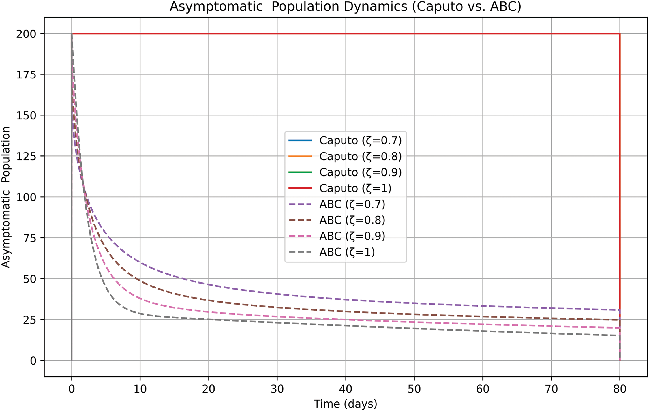
In Fig. 18, ABC model is more realistic, as it shows a decline in asymptomatic cases over time, reflecting real-world disease progression. The Caputo model is overly simplistic, keeping the asymptomatic population constant and failing to capture transitions. Higher ζ values lead to faster transitions in the ABC model, while lower ζ values indicate longer asymptomatic periods. The ABC model is preferable for understanding asymptomatic transmission dynamics, making it a better choice for modeling diseases with significant asymptomatic spread.

Figure 18: Comparison of ABC and Caputo on asymptomatic
In Fig. 19, ABC model is more realistic for modeling symptomatic cases, showing a gradual decline over time. The Caputo model fails to capture symptom resolution, making it less suitable for infectious diseases where symptoms eventually disappear. Higher ζ values lead to faster symptom resolution, while lower ζ values indicate prolonged symptomatic periods. The ABC model is preferable for tracking disease progression and recovery, making it a better choice for epidemic modeling. In Fig. 20, ABC model is better suited for modeling dynamic isolation processes. The Caputo model fails to capture the evolving nature of isolation, making it less effective for real-world outbreak simulations. Higher ζ values lead to faster isolation rates, representing stronger containment measures. The ABC model aligns better with real-world quarantine strategies, making it the preferred choice for epidemiological studies. In Fig. 21, ABC model is more suitable for epidemic modeling, as it realistically captures increasing recovery rates. The Caputo model fails to show recovery, making it unrealistic for studying disease progression. Higher ζ values lead to faster recovery, reflecting better medical care and public health interventions. The ABC model aligns better with real-world epidemiological patterns, making it the preferred model for studying outbreaks.

Figure 19: Comparison of ABC and Caputo on symptomatic

Figure 20: Comparison of ABC and Caputo on isolation

Figure 21: Comparison of ABC and Caputo on recovery
15 Conclusion
This paper presents a model for Monkeypox virus disease within the framework of the 𝒜ℬ𝒞 fractional derivative to analyze the Monkeypox disease-free equilibrium, and the equilibrium exists both locally and across all scales. The disease-free equilibrium remains stable when the basic reproduction number is below unity. When F˘0 values are below unity, the disease-free equilibrium attains local and global stability. Yet the endemic equilibrium reaches stability at both levels when F˘0 exceeds unity and is asymptotically stable when the basic reproduction number is greater than unity. Initially, we enhance the existence theory for the model, establishing both the existence and uniqueness of solutions through a fixed-point approach. Following these results, we investigate the stability of the solutions using Ulam-Hyers and Ulam-Hyers-Rassias stability criteria. Additionally, we conduct numerical experiments to validate the model, developing a numerical scheme that is subsequently utilized to generate graphical results. Our numerical simulations produce realistic graphs, which are thoroughly explained in the numerical section of the paper across various orders of the 𝒜ℬ𝒞 fractional derivatives. Thus, the model helps in formulating strategies for the attainment of Goals 3, 15, and 17 of the UN SDG. Two types of fractional derivatives based on Caputo and 𝒜ℬ𝒞 were analyzed to explain the novelty of the model. We encourage readers to explore the model further using alternative numerical techniques and different fractional operators to gain deeper insights into the Monkeypox virus disease dynamics.
Acknowledgement: The authors convey their sincere appreciation to the Prince Sattam Bin Abdulaziz University for assisting this research.
Funding Statement: This project is sponsored by Prince Sattam Bin Abulaziz University (PSAU) as part of funding for its SDG Roadmap Research Funding Programme Project Number PSAU-2023-SDG-107.
Author Contributions: The authors confirm contribution to the paper as follows: Conception: Rajagopalan Ramaswamy, Ozgur Ege; Methodology: Rajagopalan Ramaswamy, Gunaseelan Mani; Project Management: Gunaseelan Mani, Ozgur Ege; Supervision: Rajagopalan Ramaswamy; Software: Deepak Kumar; Writing—Orignial Draft: Gunaseelan Mani, Deepak Kumar; Writing—Review and Editiing: Rajagopalan Ramaswamy, Gunaseelan Mani, Ozgur Ege. All authors reviewed the results and approved the final version of the manuscript.
Availability of Data and Materials: Data sharing not applicable to this article as no datasets were generated or analyzed during the current study.
Ethics Approval: Not applicable.
Conflicts of Interest: The authors declare no conflicts of interest to report regarding the present study.
References
1. WHO recommends new name for monkeypox disease; 2023 [Internet]. [cited 2025 Apr 22]. Available from: https://www.who.int/news/item/28-11-2022-who-recommends-new-name-for-monkeypox-disease. [Google Scholar]
2. Thornhill JP, Barkati S, Walmsley S, Rockstroh J, Andrea A, Harrison LB, et al. Monkeypox virus infection in humans across 16 countries. N Engl J Med. 2022;387(8):679–91. doi:10.1056/NEJMoa2207323. [Google Scholar] [PubMed] [CrossRef]
3. Mpox (Monkeypox). key Facts, World Health Organization; 2023 [Internet]. [cited 2025 Apr 22]. Available from: https://www.who.int/news-room/fact-sheets/detail/monkeypox. [Google Scholar]
4. 2022-24 Mpox (Monkeypox) Outbreak: Global Trends, World Health Organization; 2023 [Internet]. [cited 2025 Apr 22]. Available from: https://worldhealthorg.shinyapps.io/mpx_global/#1_Overview. [Google Scholar]
5. Science brief: detection and transmission of mpox virus during the 2022 clade IIb outbreak; 2023 [Internet]. [cited 2025 Apr 22]. Available from: https://www.cdc.gov/poxvirus/mpox/about/sciencebehind-transmission.html. [Google Scholar]
6. Usman S, Adamu II. Modeling the transmission dynamics of the monkeypox virus infection with treatment and vaccination interventions. J Appl Math Phys. 2017;5(12):2335–53. doi:10.4236/jamp.2017.512191. [Google Scholar] [CrossRef]
7. Ellis CK, Carroll DS, Lash RR, Peterson AT, Damon IK, Malekani J, et al. Ecology and geography of human monkeypox case occurrences across Africa. J Wildl Dis. 2012;48(2):335–47. doi:10.7589/0090-3558-48.2.335. [Google Scholar] [PubMed] [CrossRef]
8. Philpott D. Epidemiologic and clinical characteristics of monkeypox cases in United States. MMWR Morb Mortal Wkly Rep. 2022;71(32):1018–22. doi:10.15585/mmwr.mm7132e3.. [Google Scholar] [PubMed] [CrossRef]
9. Centers for disease control and prevention. Pets in the home; 2023 [Internet]. [cited 2025 Apr 22]. Available from: https://www.cdc.gov/poxvirus/mpox/prevention/pets-in-homes.html. [Google Scholar]
10. Seang S, Burrel S, Todesco E, Leducq V, Monsel G, Le PD, et al. Evidence of human-to-dog transmission of monkeypox virus. Lancet. 2022;400(10353):658–9. doi:10.1016/S0140-6736(22)01487-8. [Google Scholar] [PubMed] [CrossRef]
11. Ackora-Prah J, Okyere S, Bonyah E, Adebanji AO, Boateng Y. Optimal control model of human-to-human transmission of monkeypox virus. F1000 Res. 2023;12:326. doi:10.12688/f1000research. [Google Scholar] [CrossRef]
12. Bankuru SV, Kossol S, Hou W, Mahmoudi P, Rychtář J, Taylor D. A game-theoretic model of Monkeypox to assess vaccination strategies. PeerJ. 2020;8(1):e9272. doi:10.7717/peerj.9272. [Google Scholar] [PubMed] [CrossRef]
13. Bhunu CP, Mushayabasa S. Modelling the transmission dynamics of pox-like infections. IAENG Int J Appl Mathemat. 2011;41(2):141–9. [Google Scholar]
14. Ngungu M, Addai E, Adeniji A, Adam UM, Oshinubi K. Mathematical epidemiological modeling and analysis of monkeypox dynamism with non-pharmaceutical intervention using real data from United Kingdom. Front Public Health. 2023;11:1101436. doi:10.3389/fpubh.2023.1101436. [Google Scholar] [PubMed] [CrossRef]
15. Somma SA, Akinwande NI, Chado UD. A mathematical model of monkey pox virus transmission dynamics. Ife J Sci. 2019;21(1):195–204. doi:10.4314/ijs.v21i1.17. [Google Scholar] [CrossRef]
16. Ahmad YU, Andrawus J, Ado A, Yahaya AM, Abdullahi Y, Saad A, et al. Mathematical modeling and analysis of human-to-human monkeypox virus transmission with post-exposure vaccination. Model Earth Syst Environ. 2024;10(2):2711–31. doi:10.1007/s40808-023-01920-1. [Google Scholar] [CrossRef]
17. Peter OJ, Oguntolu FA, Ojo MM, Olayinka OA, Jan R, Khan I. Fractional order mathematical model of monkeypox transmission dynamics. Phys Scripta. 2022;97(8):084005. doi:10.1088/1402-4896/ac7ebc. [Google Scholar] [CrossRef]
18. Al Qurashi M, Rashid S, Alshehri AM, Jarad F, Safdar F. New numerical dynamics of the fractional monkeypox virus model transmission pertaining to nonsingular kernels. Math Biosci Eng. 2023;20(1):402–36. doi:10.3934/mbe.2023019. [Google Scholar] [PubMed] [CrossRef]
19. Bansal J, Kumar A, Kumar A, Khan A, Abdeljawad T. Investigation of monkeypox disease transmission with vaccination effects using fractional order mathematical model under Atangana-Baleanu Caputo derivative. Model Earth Syst Environ. 2025;11(1):40. doi:10.1007/s40808-024-02202-0. [Google Scholar] [CrossRef]
20. Okyere S, Ackora-Prah J. Modeling and analysis of monkeypox disease using fractional derivatives. Resul Eng. 2023;17(3):100786. doi:10.1016/j.rineng.2022.100786. [Google Scholar] [PubMed] [CrossRef]
21. Liu B, Farid S, Ullah S, Altanji M, Nawaz R, Wondimagegnhu TS. Mathematical assessment of monkeypox disease with the impact of vaccination using a fractional epidemiological modeling approach. Sci Rep. 2023;13(1):13550. doi:10.1038/s41598-023-40745-x. [Google Scholar] [PubMed] [CrossRef]
22. Atangana A, Baleanu D. New fractional derivatives with non-local and non-singular kernel: theory and application to heat transfer model. Therm Sci. 2016;20(2):763–9. doi:10.2298/TSCI160111018A. [Google Scholar] [CrossRef]
23. Podlubny I. Fractional differential equations: an introduction to fractional derivatives, fractional differential equations, to methods of their solution and some of their applications. Amsterdam, Netherlands: Elsevier; 1998. [Google Scholar]
24. Banach S. Sur les opérations dans les ensembles abstraits et leur application auxéquations intégrales. Fundam Math. 1922;3:133–81. doi:10.4064/fm-3-1-133-181. [Google Scholar] [PubMed] [CrossRef]
25. DeJesus EX, Kaufman C. Routh-Hurwitz criterion in the examination of eigenvalues of a system of nonlinear ordinary differential equations. Phys Rev A. 1987;35(12):5288. doi:10.1103/PhysRevA.35.5288. [Google Scholar] [PubMed] [CrossRef]
26. Castillo-Chavez C, Song B. Dynamical models of tuberculosis and their applications. Math Biosci Eng. 2004;1(2):361–404. doi:10.3934/mbe.2004.1.361. [Google Scholar] [PubMed] [CrossRef]
27. La Salle JP. The stability of dynamical systems. In: Regional Conference Series in Applied Mathematics. Philadelphia, PA, USA: SIAM; 1976. [Google Scholar]
28. Vargas-De-Leon C, d’Onofrio A. Global stability of infectious disease models with contact rate as a function of prevalence index. Math Biosci Eng. 2017;14(4):1019–33. doi:10.3934/mbe.2017053. [Google Scholar] [PubMed] [CrossRef]
29. Balasubramaniam P, Prakash M, Rihan FA, Lakshmanan S. Hopf bifurcation and stability of periodic solutions for delay differential model of HIV infection of CD4+ T-cells. Abstr Appl Anal. 2014;2014(2):1–19. doi:10.1155/2014/838396. [Google Scholar] [CrossRef]
30. Olaniyi S, Lawal MA, Obabiyi OS. Stability and sensitivity analysis of a deterministic epidemiological model with pseudo-recovery. IAENG Int J Appl Math. 2016;46(2):160–7. [Google Scholar]
31. Andrawus J, Ahmad YU, Andrew AA, Yusuf AA, Qureshi S, Denue BA. Impact of surveillance in human-to-human transmission of monkeypox virus. Eur Phys J Spec Top. 2024;22(6):1014. doi:10.1140/epjs/s11734-024-01346-5. [Google Scholar] [CrossRef]
32. Kumar S, Kumar A, Jleli M. A numerical analysis for fractional model of the spread of pests in tea plants. Numer Methods Partial Differential Eqs. 2022;38(3):540–65. doi:10.1002/num.22663. [Google Scholar] [CrossRef]
33. Kumar S, Kumar A, Samet B, Dutta H. A study on fractional host-parasitoid population dynamical model to describe insect species. Numer Methods Partial Differential Eqs. 2021;37(2):1673–92. doi:10.1002/num.22603. [Google Scholar] [CrossRef]

 Submit a Paper
 Propose a Special lssue
 Open Access
 View Full Text
 Download PDF


 Copyright © 2025 The Author(s). Published by Tech Science Press.
 Downloads
 Citation Tools