
 Submit a Paper
 Propose a Special lssue
 Open Access
ARTICLE

Analysis of a Laplace Spectral Method for Time-Fractional Advection-Diffusion Equations Incorporating the Atangana-Baleanu Derivative
1 Department of Mathematics, Islamia College Peshawar, Peshawar, Khyber Pakhtoon Khwa, 25120, Pakistan
2 Department of Mathematics, College of Science, King Khalid University, Abha, 61413, Saudi Arabia
3 Centro de Investigación en Ingenierìa y Ciencias Aplicadas (CIICAp-IICBA)/UAEM, Universidad Autónoma del Estado de Morelos, Av. Universidad 1001. Col. Chamilpa, Cuernavaca, 62209, Morelos, México
4 Department of Mathematical Sciences, Princess Nourah Bint Abdulrahman University, Riyadh, 11671, Saudi Arabia
5 Department of Computing, Mathematics and Electronics, “1 Decembrie 1918” University of Alba Iulia, Alba Iulia, 510009, Romania
6 Faculty of Mathematics and Computer Science, Transilvania University of Brasov, Iuliu Maniu Street 50, Brasov, 500091, Romania
* Corresponding Authors: Kamran. Email: ; Ioan-Lucian Popa. Email:
(This article belongs to the Special Issue: Analytical and Numerical Solution of the Fractional Differential Equation)
Computer Modeling in Engineering & Sciences 2025, 143(3), 3433-3462. https://doi.org/10.32604/cmes.2025.064815
Received 25 February 2025; Accepted 07 May 2025; Issue published 30 June 2025
 View Full Text
 Download PDF
Abstract
In this article, we develop the Laplace transform (LT) based Chebyshev spectral collocation method (CSCM) to approximate the time fractional advection-diffusion equation, incorporating the Atangana-Baleanu Caputo (ABC) derivative. The advection-diffusion equation, which governs the transport of mass, heat, or energy through combined advection and diffusion processes, is central to modeling physical systems with nonlocal behavior. Our numerical scheme employs the LT to transform the time-dependent time-fractional PDEs into a time-independent PDE in LT domain, eliminating the need for classical time-stepping methods that often suffer from stability constraints. For spatial discretization, we employ the CSCM, where the solution is approximated using Lagrange interpolation polynomial based on the Chebyshev collocation nodes, achieving exponential convergence that outperforms the algebraic convergence rates of finite difference and finite element methods. Finally, the solution is reverted to the time domain using contour integration technique. We also establish the existence and uniqueness of the solution for the proposed problem. The performance, efficiency, and accuracy of the proposed method are validated through various fractional advection-diffusion problems. The computed results demonstrate that the proposed method has less computational cost and is highly accurate.Keywords
Fractional calculus (FC) is a historical discipline in mathematics that traces its origins to the works of Leibniz and Euler, who explored integrals and derivatives of non-integer orders [1]. Despite significant advancements, this topic continues to captivate researchers due to its rich mathematical and numerical aspects. Today, FC extends beyond pure mathematics and has found applications in various scientific disciplines [2]. Replacing standard operators with fractional operators has significantly enhanced the precision and accuracy of numerous physical models and systems [3–5]. Researchers have explored numerous fractional operators and assessed various definitions of fractional derivatives, particularly those governed by power-law kernels, commonly known as singular or local fractional derivatives. Notable examples include the Grünwald-Letnikov, Riemann-Liouville, Caputo, Riesz, and Hadamard fractional derivatives [6]. However, these fractional derivatives can efficiently model the non-local and dissipative properties of physical processes. The non-locality of a fractional derivative refers to the fact that the value of a fractional derivative at a given point depends on the function’s values over an entire interval rather than just at the point itself.
In 2015, Caputo and Fabrizio [7] introduced a new fractional derivative, termed the Caputo-Fabrizio (CF) derivative, which employs an exponential kernel to overcome the limitations of fractional derivatives with singular kernels, such as those found in the Riemann-Liouville and Liouville-Caputo derivatives. The singularity in these earlier definitions often complicates their application to physical systems. The CF derivative’s exponential kernel, being nonsingular, provides a more natural transition and eliminates the issues associated with the Riemann-Liouville and Liouville-Caputo derivatives. However, despite its innovation, the CF derivative faced criticisms for a notable drawback: its kernel lacks nonlocality. To address these shortcomings, Atangana and Baleanu [8] introduced a novel fractional derivative in 2016, known as Atangana-Baleanu (AB) derivative, which is based on the Mittag-Leffler function. Unlike the CF derivative the AB derivative incorporates a nonlocal and nonsingular kernel, effectively combining the strengths of the Riemann-Liouville, Liouville-Caputo, and Caputo-Fabrizio derivatives. The AB derivative provides several advantages: (i) its nonlocal nature guarantees that it captures the full historical behavior of the function being differentiated; (ii) it has an adjustable parameter, that lets researchers change the fractional order to enhance data-fitting accuracy; (iii) the AB derivative exhibits greater flexibility than its predecessor’s derivatives, enabling accurate modeling of complex systems; and (iv) it offers a unifying structure that can refine and improve the existing models across various scientific domains by integrating the features of the Riemann-Liouville, Liouville-Caputo and extending their applicability. Due to these compelling attributes, the AB derivative has gained significant attention and has been successfully applied to a wide range of real-world problems [9].
Time-fractional advection-diffusion equations (TFADEs) are widely used models in applied mathematics to describe various physical systems. The advection term represents the movement of a fluid along a concentration gradient, while the diffusion term describes the process by which material spreads from regions of higher to lower concentration over time. TFADEs are applied to transport processes, including the long-range dispersion of air pollutants [10], turbulence [11], water transport in soil [12], dispersion in porous media [13], shallow water flow [14], ion transport in heterogeneous media [15], blood flow with chemical interactions [16], and contaminant transport in soil [17].
Analytical solutions for TFADEs have been derived by various researchers. For example, Sanskrityayn and Kumar [18] derived analytical solutions to TFADEs using Green’s function methods. Avci and Yetim [19] obtained analytical solutions for TFADEs incorporating the Atangana-Baleanu fractional derivative, while Mirza and Vieru [20] derived fundamental solutions for TFADEs using the Caputo-Fabrizio derivative. However, obtaining exact solutions for TFADEs is often challenging due to the involvement of complex functions, which can be difficult to handle analytically.
As a result, developing accurate and efficient numerical schemes has become essential. Many authors in the literature have proposed numerical solutions for TFADEs. Umer et al. [21] analyzed numerical solutions of advection-diffusion equations with the Atangana-Baleanu fractional derivative using an extended cubic B-spline technique. Fazio et al. [22] studied a finite difference method on non-uniform meshes for TFADEs with a source term. Ahmed et al. [23] applied a Haar wavelet-based numerical technique to solve TFADEs. Kamran et al. [24] investigated numerical inverse Laplace transform methods for approximating TFADEs.
Other contributions include the work by Pareek et al. [25], who developed the natural transform method for solving TFADEs, and Chawla et al. [26], who utilized extended one-step time integration schemes. Liu et al. [27] proposed a radial basis function (RBF)-based differential quadrature method for solving two-dimensional TFADEs. Nguyen and Reynen [28] devised a space-time least squares finite element scheme for approximating TFADEs, while Cunha et al. [29] employed the boundary element method to solve TFADEs. Sweilam et al. [30] simulated TFADEs using a spectral collocation method combined with a non-standard finite difference technique.
Many authors have developed and modified numerical methods for the approximation of fractional partial differential equations (FPDEs) from various perspectives, focusing on improving accuracy, stability, efficiency, consistency, and performance in terms of computational cost. In recent years, hybrid methods have gained significant attention due to their high accuracy, low computational cost, and ease of implementation for discretizing FPDEs.
Hybrid methods combine two or more approaches, enabling them to mitigate the limitations of individual methods. As a result, hybrid methods can approximate complex problems in a simple and effective manner. In the literature, several researchers have proposed hybrid methods. For example, Yin et al. [31] combined the Laplace transform and Legendre wavelet methods for the numerical simulation of Klein-Gordon equations. Soares and Mansur [32] coupled the boundary element method with the finite element method for solving acoustic elastodynamic problems. A hybrid method based on the Laplace transform and Legendre wavelet approaches was analyzed in [33] for the approximation of Lane-Emden equations. Khan et al. [34] combined the homotopy perturbation method with the Laplace transform method to solve fractional models. Joujehi et al. [35] developed a hybrid method based on Beta functions and fractional-order Bernoulli wavelets for approximating multi-term TFPDEs in fluid mechanics. A review of the Jacobi-Galerkin spectral method for linear partial differential equations is examined by Hafez and Youssri [36]. Lim and Li [37] coupled the boundary element method with the finite difference method to approximate fluid-structure interaction problems with dynamic analysis of outer hair cells. Kamran et al. [38] combined the Laplace transform with radial basis functions for the numerical approximation of the mobile-immobile advection-dispersion problem arising in solute transport. Sahu and Jena [39] developed an efficient technique for time fractional Klein-Gordon equation based on modified Laplace Adomian decomposition technique via hybridized Newton-Raphson Scheme arises in relativistic fractional quantum mechanics.
The main objective of this work is to develop and analyze a hybrid Laplace Transform-based Chebyshev Spectral Collocation Method (LT-CSCM) for the efficient numerical solution of time-fractional advection-diffusion equations (TFADEs) featuring a nonsingular kernel. By combining the LT for temporal discretization with the CSCM for spatial discretization, our method aims to achieve high accuracy and computational efficiency.
The CSCM is a subclass of spectral methods that has recently garnered significant attention due to its straightforward implementation for the spatial approximation of fractional partial differential equations (FPDEs). Within the numerical framework for FPDEs, CSCM belongs to the family of Weighted Residual Methods (WRMs) [40]. This family includes the Tau, Galerkin, and collocation methods, each employing distinct techniques to minimize residuals. In the Galerkin and Tau methods, residuals are projected onto a polynomial space and constrained to be zero, while the collocation method enforces zero residuals at specific grid points. For FPDEs, Chebyshev collocation points are highly effective as grid points due to their optimal distribution, which enhances numerical accuracy. CSCM utilizes basis functions, typically Lagrange interpolation polynomials, defined at these points [41]. This global approach achieves spectral convergence, delivering high accuracy for problems with simple geometries and smooth solutions [42,43]. Compared to finite difference or finite element methods, CSCM is easier to implement and significantly reduces computational cost.
The CSCMs have been widely adopted by numerous researchers for many applications. Such as Khader and Saad [44] utilized the CSCM for the solution of the fractional Fisher problems. In [45], the authors proposed approximating fractional-order diffusion problems using CSCM combined with a power-series method based on residuals. The authors of [46] obtained the solution of the time-fractional advection-diffusion equation using CSCM. Tohidi [47] developed a numerical scheme for finding approximate solutions of one-dimensional parabolic partial differential equations (PDEs) under non-classical boundary conditions. In [48], the authors proposed a spectral collocation method based on differentiated Chebyshev polynomials to obtain numerical solutions for various types of nonlinear partial differential equations. Li et al. [49] employed the CSCM to solve the transport equation with given initial and boundary conditions. Rongpei et al. [50] solved two-dimensional nonlinear reaction-diffusion equations with Neumann boundary conditions using a new highly accurate CSCM.
The LT is an efficient and error-free method for the temporal discretization of FPDEs, addressing stability issues often encountered with traditional time-marching methods. These methods are stable and accurate only if the error calculated in a one-time step does not amplify as computations progress. In other words, time-marching methods remain stable if the error diminishes or remains unchanged during computations. Moreover, achieving optimal accuracy with time-marching methods typically requires smaller time steps, which significantly increases computational cost [51], thus affecting the overall efficiency of the method. One of its key advantages is its ability to convert differential equations into algebraic equations, making complex problems more manageable. Additionally, it provides a systematic approach for handling initial conditions directly within the transformed domain, avoiding the need for numerical time-stepping methods that may suffer from stability issues [52]. The LT is particularly beneficial for solving linear time-invariant systems and fractional differential equations, as it allows for analytical solutions in many cases [53]. However, the method also has limitations. It is less effective for nonlinear problems, as transforming the nonlinear terms is not straightforward, often requiring approximations or numerical techniques [54]. By employing the LT for temporal discretization, the FPDEs are transformed into the Laplace domain. To obtain the solution in the time domain, the inverse Laplace transform (ILT) must be applied. However, the exact computation of Evaluating the Bromwich integral is computationally complex, prompting the adoption of numerical inverse Laplace transform methods (ILTMs). Several authors have developed numerical ILTMs. For instance: De Hoog et al. [55] employed the quotient-difference scheme to formulate an improved ILTM that accelerates Fourier series convergence. Stehfest [56] developed a linear acceleration method using Salzer’s approach for numerical inversion of the LT. Talbot [57] introduced an efficient ILTM. Weideman and Trefethen [58] utilized parabolic and hyperbolic contours to approximate the Bromwich integral. Weeks [59] employed Laguerre functions for numerical ILTM. Each numerical method for inverting the Laplace transform has specific applications and is best suited to a particular problem. Contour integration methods, such as those based on hyperbolic, parabolic, or Talbot contours, are particularly effective for partial differential equations (PDEs) due to their ease of implementation and high accuracy. These methods deform the integration path in the complex plane to optimize convergence, minimizing computational complexity while maintaining precision. In this work, we utilize the numerical ILTMs described in [58,60]. Consider the following 2-D TFADE:
where,
with
and
2 Existence and Uniqueness of the Solution
In this section, we utilize the fixed-point theory to prove the existence and uniqueness of the solution to the fractional advection-diffusion model (1). Let us define a Banach space
Let define the operator
The fixed point of
Theorem 1. If assumptions
Proof. The proof consists of several steps.
Step 1: Continuity of
Since
Therefore,
Step 2: Boundedness of
Defining
it follows that
Step 3: Equicontinuity of
It follows that
By the Arzelà-Ascoli Theorem [61], the operator
Step 4: A Priori Bound. Define
Now, using assumptions
which gives
where
Theorem 2. The problem define in Eq. (1) has a unique solution if the assumptions
Proof
Thus, we find that under the given assumptions
In the LT-CSCM approach, the Laplace Transform (LT) transforms Eq. (1) into the Laplace domain, enabling efficient temporal discretization. The Chebyshev Spectral Collocation Method (CSCM) is then applied to discretize spatial variables with high accuracy. Finally, the time-domain solution is recovered using the Talbot method for numerical inverse Laplace transform, ensuring precision and computational efficiency.
The Laplace Transform is used for the temporal discretization of the proposed problem defined in Eq. (1). The LT of
The LT of the ABC derivative,
Applying the LT to Eq. (1) yields
and
Simplifying further, we obtain
and
where
and I is the
3.2 Spatial Discretization by Chebyshev Spectral Collocation Method
In CSCM, a global polynomial interpolant is utilized on specific nodes (Chebychev nodes) to approximate the unknown solution of a FPDEs. The spatial derivatives are computed using discrete derivative operators, also called differentiation matrices (DM) [41].
The solution is considered over
where
For spatial discretization in
The first derivative
where
The non-diagonal entries of
where
The elements of the DM,
More efficient elaboration of the differentiation matrices can be found in [62]. Welfert [41], obtained an easy to use recursion relation for the calculation of differentiation matrix, as follows:
For the square domain
The basic Lagrange polynomials associated to
with
where
Finally, the approximation of
By using Eq. (14) in Eq. (8), we get
In order to incorporate the boundary conditions in Eq. (9), we consider
where H is the square matrix of order
where the values of interior-boundary points are accumulated via
Error Bound of CSCM
As
For the calculation of the error bound of CSCM, we utilze the work of Börm et al. [63]. Suppose for all
Furthermore, for all
For interpolation based on Chebyshev points, we have
The stability constant get larger very sluggishly [63], the approximation bound is given as
Theorem 3 [63]. If the polynomial interpolation error bound in (17) and the approximation bound in (20) hold for all
where
The error bound is formulated by utilizing the results in Eq. (20) and Eq. (21), for
the time derivatives is computed precisely, so the bound of error of
where
3.3 Numerical Inverse Laplace Transform Methods
We utilize the ILTMs for inversion of the solution obtained through CSCM in the Laplace space to time domain. The solution
where
The
For
where
The parametric form of
with
Now, using
and the integral in Eq. (26) can be approximated using the trapezoidal rule, resulting in
This section addresses the error analysis of the LT-CSCM. The Laplace transform is applied in the first step, which is inherently free of error. The CSCM is employed in the second step for approximating the solution of the transformed problem. The following theorem establishes the error bounds of the CSCM.
Theorem 4 (Theorem 5, pp. 48, [42]). Let
where
For every
suppose for
The above estimate is valid for any order derivatives
Finally, we employ the ILTMs in order to approximate the Eq. (27). While approximating Eq. (27) the convergence of the proposed scheme depends on
The error of the
the finite approximations are
and the infinite approximations are
The discretization error is given by
Theorem 5 [58]. Let
Then, we have
If
To get an estimation of
The estimate of error is
The parameter
Similarly, the estimation of the discretization error for the hyperbolic contour is presented in the following theorem.
Theorem 6 ([60], Theorem 2). Let
In the current work, we use the optimal contour of integration with the parameters given in Eq. (25) are suggested by McLean and Thomèe [60] as
and the error estimate is given as
To analyze the stability of our numerical scheme, we express the system defined in (8) and (9) in its discrete form as follows:
where
The value of
In terms of pseudoinverse
Hence, we have the following bound:
Eqs. (31) and (33) establish bounds for the constant
This approach performs well for our differentiation matrix

Figure 1: (a) The plot of the stability constant
We consider three different test examples to validate and check the efficiency of the LT-CSCM. The maximum absolute error norm is computed among the numerical solutions and the analytical solutions. The error norm is defined as
where
Example 1
Consider a 2D TFADE in Eq. (1) with exact solution
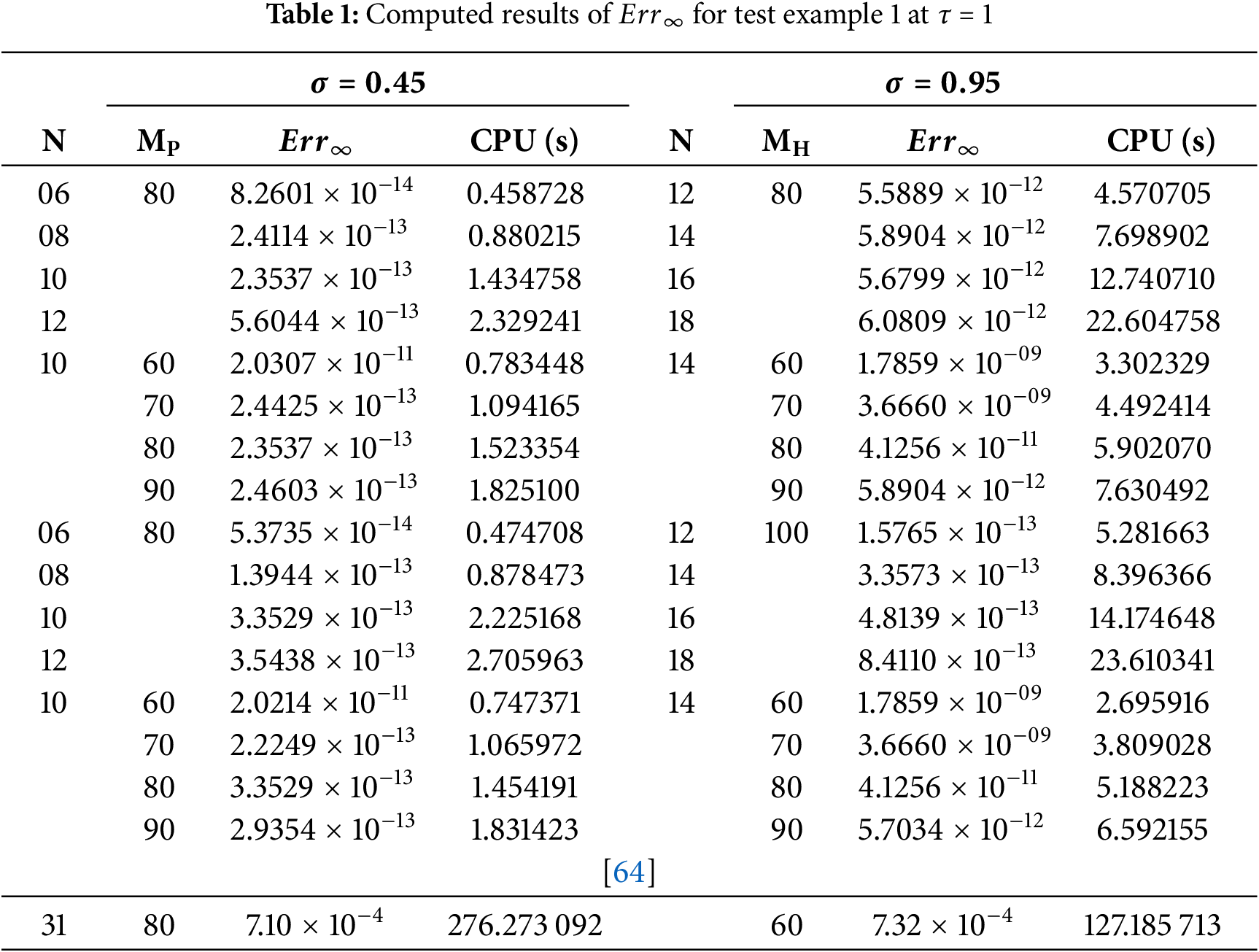
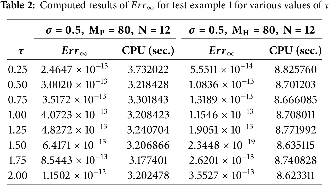

Figure 2: (a) Numerical solution of test example

Figure 3: (a) The Plots shows

Figure 4: (a) We have plotted the error as a function of
Example 2
Consider a 2D TFADE defined in Eq. (1) with exact solution
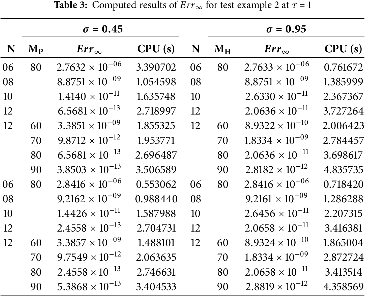


Figure 5: (a) Numerical solution of test example

Figure 6: (a) The Plots shows

Figure 7: (a) We have plotted the error as a function of
Example 3
Consider a 2D TFADE in Eq. (1) with exact solution


Figure 8: (a) Numerical solution of test example

Figure 9: (a) The Plots shows

Figure 10: (a) We have plotted the error as a function of
In this study, we developed a LT-CSCM to solve time-fractional advection-diffusion equations including the AB derivative with high accuracy and computational efficiency. By integrating the LT with the CSCM, our approach combines the advantages of both approaches: the Laplace transform eliminates time-stepping complexities, ensuring exact temporal discretization, while the CSCM, utilizing Lagrange polynomials-based on Chebyshev nodes, achieves exponential convergence in the spatial domain with minimal nodes. This combination results in low computational cost and high accuracy, as demonstrated by the excellent agreement between our numerical results and exact solutions across various test cases. Despite these advantages, we acknowledge certain limitations. The CSCM’s reliance on global basis functions can pose challenges for problems involving irregular geometries or complex boundary conditions, where local methods might be more adaptable. Furthermore, the global nature of the approach may limit its adaptability to very large-scale problems. To revert solutions from the Laplace domain to the time domain, we employed a numerical inverse Laplace transform, which maintained stability and accuracy throughout. Overall, the LT-CSCM proves to be a robust and efficient tool for time-fractional advection-diffusion problems, with the potential for further refinement to address complex geometries and broader applications. As a future direction, we aim to extend the proposed LT-CSCM framework to solve multi-dimensional time-fractional problems and to compare the performance and accuracy of the method when applied to different types of fractional derivatives, including the modified Atangana-Baleanu derivative. This will enable a deeper understanding of the method’s adaptability and effectiveness across various fractional models and more realistic physical phenomena.
Acknowledgement: The authors extend their appreciation to the Deanship of Research and Graduate Studies at King Khalid University for funding this work through Large Research Project under grant number RGP2/174/46.
Funding Statement: The authors extend their appreciation to the Deanship of Research and Graduate Studies at King Khalid University for funding this work through Large Research Project under grant number RGP2/174/46.
Author Contributions: Kamran: Conceptualization, methodology, validation, investigation, writing—original draft, visualization, supervision, writing—review and editing. Farman Ali Shah: methodology, software, writing—original draft, data curation, writing—review and editing. Kallekh Afef: validation, formal analysis, investigation, writing—review and editing, project administration. J. F. Gómez-Aguilar: investigation, data curation, visualization, writing—review and editing. Salma Aljawi: validation, investigation, formal analysis, resources. Ioan-Lucian Popa: formal analysis, investigation, visualization, funding acquisition. All authors reviewed the results and approved the final version of the manuscript.
Availability of Data and Materials: All the data produced or examined in this study are provided within this article.
Ethics Approval: There does not exist any ethical issue regarding this work.
Conflicts of Interest: The authors declare no conflicts of interest to report regarding the present study.
References
1. Sun H, Zhang Y, Baleanu D, Chen W, Chen Y. A new collection of real world applications of fractional calculus in science and engineering. Commun Nonlinear Sci Numer Simul. 2018;64:213–31. doi:10.1016/j.cnsns.2018.04.019. [Google Scholar] [CrossRef]
2. Podlubny I. Fractional differential equations. San Diego, CA, USA: Academic Press; 1998. [Google Scholar]
3. Abdeljawad T, Baleanu D. Discrete fractional differences with nonsingular discrete Mittag-Leffler kernels. Adv Differ Equ. 2016;2016:1–18. doi:10.1186/s13662-016-0949-5. [Google Scholar] [CrossRef]
4. Jena SR, Sahu I. A novel approach for numerical treatment of traveling wave solution of ion acoustic waves as a fractional nonlinear evolution equation on Shehu transform environment. Phys Scr. 2023;98(8):085231. doi:10.1088/1402-4896/ace6de. [Google Scholar] [CrossRef]
5. Li C, Guo H, Tian X, He T. Generalized thermoelastic diffusion problems with fractional order strain. Eur J Mech-A/Solids. 2019;78:103827. doi:10.1016/j.euromechsol.2019.103827. [Google Scholar] [CrossRef]
6. Kilbas AA, Srivastava HM, Trujillo JJ, Theory and applications of fractional differential equations. Vol. 204. Amsterdam, The Netherland: Elsevier; 2006. [Google Scholar]
7. Caputo M, Fabrizio M. A new definition of fractional derivative without singular kernel. Prog Fract Differ Appl. 2015;1(2):73–85. doi:10.12785/pfda/010201. [Google Scholar] [CrossRef]
8. Atangana A, Baleanu D. New fractional derivatives with nonlocal and non-singular kernel: theory and application to heat transfer model. Therm Sci. 2016;20(2):763. doi:10.2298/TSCI160111018A. [Google Scholar] [CrossRef]
9. Hristov J. On the Atangana-Baleanu derivative and its relation to the fading memory concept: the diffusion equation formulation. Fractional derivatives with mittag-leffler kernel: trends and applications in science and engineering. 1st ed. Cham, Switzerland: Springer; 2019. p. 175–93. doi:10.32604/iasc.2023.032883. [Google Scholar] [CrossRef]
10. Zlatev Z, Berkowicz R, Prahm LP. Implementation of a variable stepsize variable formula method in the time-integration part of a code for treatment of long-range transport of air pollutants. J Comput Phys. 1984;55(2):278–301. doi:10.1016/0021-9991(84)90007-X. [Google Scholar] [CrossRef]
11. Bakunin OG. Turbulence and diffusion: scaling vs. equations. Berlin/Heidelberg, Germany: Springer Science & Business Media; 2008. doi:10.1007/978-3-540-68222-6. [Google Scholar] [CrossRef]
12. Sun L, Qiu H, Wu C, Niu J, Hu BX. A review of applications of fractional advection-dispersion equations for anomalous solute transport in surface and subsurface water. Wiley Interdiscip Rev: Water. 2020;7(4):e1448. doi:10.1002/wat2.1448. [Google Scholar] [CrossRef]
13. Da Silva JRD, Xavier PHF, Moreira DM. Near-field atmospheric dispersion modeling: a new approach for the two-dimensional steady-state advection-diffusion equation using fractal derivative. Pure Appl Geophys. 2025;182(1):223–33. doi:10.1007/s00024-024-03624-8. [Google Scholar] [CrossRef]
14. Budinski L. Solute transport in shallow water flows using the coupled curvilinear Lattice Boltzmann method. J Hydrol. 2019;573:557–67. doi:10.1016/j.jhydrol.2019.03.094. [Google Scholar] [CrossRef]
15. Gupta R, Kumar S. Chebyshev spectral method for the variable-order fractional mobile-immobile advection-dispersion equation arising from solute transport in heterogeneous media. J Eng Math. 2023;142(1):1–28. doi:10.1007/s10665-023-10288-1. [Google Scholar] [CrossRef]
16. Zhang H, Misbah C. Lattice Boltzmann simulation of advection-diffusion of chemicals and applications to blood flow. Comput Fluids. 2019;187:46–59. doi:10.1016/j.compfluid.2019.04.018. [Google Scholar] [CrossRef]
17. Moranda A, Cianci R, Paladino O. Analytical solutions of one-dimensional contaminant transport in soils with source production-decay. Soil Systems. 2018;2(3):40. doi:10.3390/soilsystems2030040. [Google Scholar] [CrossRef]
18. Sanskrityayn A, Kumar N. Analytical solution of advection-diffusion equation in heterogeneous infinite medium using Green’s function method. J Earth Sys Sci. 2016;125:1713–23. doi:10.1007/s12040-016-0756-0. [Google Scholar] [CrossRef]
19. Avci D, Yetim A. Analytical solutions to the advection-diffusion equation with the Atangana-Baleanu derivative over a finite domain. Balikesir Universitesi Fen Bilimleri Enstitusu Dergisi. 2018;20(2):382–95. doi:10.25092/baunfbed.487074. [Google Scholar] [CrossRef]
20. Mirza IA, Vieru D. Fundamental solutions to advection-diffusion equation with time-fractional Caputo-Fabrizio derivative. Comput Math Appl. 2017;73(1):1–10. doi:10.1016/j.camwa.2016.09.026. [Google Scholar] [CrossRef]
21. Umer A, Abbas M, Shafiq M, Abdullah FA, De la Sen M, Abdeljawad T. Numerical solutions of Atangana-Baleanu time-fractional advection diffusion equation via an extended cubic B-spline technique. Alex Eng J. 2023;74:285–300. doi:10.1016/j.aej.2023.05.028. [Google Scholar] [CrossRef]
22. Fazio R, Jannelli A, Agreste S. A finite difference method on non-uniform meshes for time-fractional advection-diffusion equations with a source term. Appl Sci. 2018;8(6):960. doi:10.3390/app8060960. [Google Scholar] [CrossRef]
23. Ahmed S, Jahan S, Nisar KS. Haar wavelet based numerical technique for the solutions of fractional advection diffusion equations. J Math Comput Sci. 2024;34(3):217–33. doi:10.22436/jmcs.034.03.02. [Google Scholar] [CrossRef]
24. Kamran, Shah FA, Aly WHF, Aksoy H, Alotaibi FM, Mahariq I. Numerical inverse laplace transform methods for advection-diffusion problems. Symmetry. 2022;14(12):2544. doi:10.3390/sym14122544. [Google Scholar] [CrossRef]
25. Pareek N, Gupta A, Agarwal G, Suthar DL. Natural transform along with HPM technique for solving fractional ADE. Adv Math Phys. 2021;2021(1):9915183. doi:10.1155/2021/9915183. [Google Scholar] [CrossRef]
26. Chawla MM, Al-Zanaidi MA, Al-Aslab M. Extended one-step time-integration schemes for convection-diffusion equations. Comput Math Appl. 2000;39(3–4):71–84. doi:10.1016/S0898-1221(99)00334-X. [Google Scholar] [CrossRef]
27. Liu J, Li X, Hu X. A RBF-based differential quadrature method for solving two-dimensional variable-order time fractional advection-diffusion equation. J Comput Phys. 2019;384:222–38. doi:10.1016/j.jcp.2018.12.043. [Google Scholar] [CrossRef]
28. Nguyen H, Reynen J. A space-time least-square finite element scheme for advection-diffusion equations. Comput Methods Appl Mech Eng. 1984;42(3):331–42. doi:10.1016/0045-7825(84)90012-4. [Google Scholar] [CrossRef]
29. Cunha CLN, Carrer JAM, Oliveira MF, Costa VL. A study concerning the solution ofadvection-diffusion problems by the Boundary Element Method. Eng Anal Bound Elem. 2016;100(65):79–94. doi:10.1016/j.enganabound.2016.01.002. [Google Scholar] [CrossRef]
30. Sweilam NH, El-Sayed AAE, Boulaaras S. Fractional-order advection-dispersion problem solution via the spectral collocation method and the non-standard finite difference technique. Chaos Solitons Fractals. 2021;144:110736. doi:10.1016/j.chaos.2021.110736. [Google Scholar] [CrossRef]
31. Yin F, Song J, Lu F. A coupled method of Laplace transform and Legendre wavelets for nonlinear Klein-Gordon equations. Math Methods Appl Sci. 2014;37(6):781–92. doi:10.1002/mma.2834. [Google Scholar] [CrossRef]
32. Soares D Jr, Mansur WJ. An efficient time-domain BEM/FEM coupling for acoustic-elastodynamic interaction problems. Comput Model Eng Sci. 2005;8(2):153–64. doi:10.3970/cmes.2005.008.153. [Google Scholar] [CrossRef]
33. Yin F, Song J, Lu F, Leng H. A coupled method of Laplace transform and Legendre wavelets for Lane-Emden-type differential equations. J Appl Math. 2012;2012(1):163821. doi:10.1155/2012/163821. [Google Scholar] [CrossRef]
34. Khan Y, Faraz N, Kumar S, Yildirim A. A coupling method of homotopy perturbation and Laplace transformation for fractional models. Univ Politehnica Bucharest Scientific Bulletin Series A Appl Math Phy. 2012;74(1):57–68. [Google Scholar]
35. Joujehi AS, Derakhshan MH, Marasi HR. An efficient hybrid numerical method for multi-term time fractional partial differential equations in fluid mechanics with convergence and error analysis. Commun Nonlinear Sci Numer Simul. 2022;114:106620. doi:10.1016/j.cnsns.2022.106620. [Google Scholar] [CrossRef]
36. Hafez RM, Youssri YH. Review on Jacobi-Galerkin spectral method for linear PDEs in applied mathematics. Contemp Math. 2024;5(2):2051–88. doi:10.37256/cm.5220244768. [Google Scholar] [CrossRef]
37. Lim KM, Li H. A coupled boundary element/finite difference method for fluid-structure interaction with application to dynamic analysis of outer hair cells. Comput Struct. 2007;85(11–14):911–22. doi:10.1016/j.compstruc.2007.01.003. [Google Scholar] [CrossRef]
38. Kamran, Khan S, Alhazmi SE, Alotaibi FM, Ferrara M, Ahmadian A. On the numerical approximation of mobile-immobile advection-dispersion model of fractional order arising from solute transport in porous media. Fractal Fract. 2022;6(8):445. doi:10.3390/fractalfract6080445. [Google Scholar] [CrossRef]
39. Sahu I, Jena SR. An efficient technique for time fractional Klein-Gordon equation based on modified Laplace Adomian decomposition technique via hybridized Newton-Raphson Scheme arises in relativistic fractional quantum mechanics. Partial Differ Equ Appl Math. 2024;10:100744. doi:10.1016/j.padiff.2024.100744. [Google Scholar] [CrossRef]
40. Boyd JP. Chebyshev and fourier spectral methods. 2nd ed. North Chelmsford, MA, USA: Courier Corporation; 2001. [Google Scholar]
41. Welfert BD. Generation of pseudospectral differentiation matrices I. SIAM J Numer Anal. 1997;34(4):1640–57. doi:10.1137/S0036142993295545. [Google Scholar] [CrossRef]
42. Trefethen LN. Spectral methods in MATLAB (Software, Environments, and Tools). Philadelphia, PA, USA: SIAM; 2000. [Google Scholar]
43. Bueno-Orovio A, Perez-Garcia VM, Fenton FH. Spectral methods for partial differential equations in irregular domains: the spectral smoothed boundary method. SIAM J Sci Comput. 2006;28(3):886–900. doi:10.1137/040607575. [Google Scholar] [CrossRef]
44. Khader MM, Saad KM. A numerical approach forsolving the fractional Fisher equation using Chebyshev spectral collocation method. Chaos Solitons Fractals. 2018;110:169–77. doi:10.1016/j.chaos.2018.03.018. [Google Scholar] [CrossRef]
45. Bayrak MA, Demir A, Ozbilge E. Numerical solution of fractional diffusion equation by Chebyshev collocation method and residual power series method. Alex Eng J. 2020;59:4709–17. doi:10.1016/j.aej.2020.08.033. [Google Scholar] [CrossRef]
46. Shokri A, Mirzaei S. A pseudo-spectral based method for time-fractional advection-diffusion equation. Comput Methods Differ Equ. 2020;8:454–67. doi:10.22034/cmde.2020.29307.1414. [Google Scholar] [PubMed] [CrossRef]
47. Tohidi E. Application of Chebyshev collocation method for solving two classes of non-classical parabolic PDEs. Ain Shams Eng J. 2015;6(1):373–9. doi:10.1016/j.asej.2014.10.021. [Google Scholar] [CrossRef]
48. Khater AH, Temsah RS, Hassan M. A Chebyshev spectral collocation method for solving Burger’s-type equations. J Comput Appl Math. 2008;222(2):333–50. doi:10.1016/j.cam.2007.11.007. [Google Scholar] [CrossRef]
49. Li Z, Chen X, Qiu J, Xia T. A novel Chebyshev-collocation spectral method for solving the transport equation. J Ind Manag Optim. 2021;17(5):2519–26. doi:10.3934/jimo.2020080. [Google Scholar] [CrossRef]
50. Rongpei Z, Mingjun L, Xijun Y. An efficient Chebyshev spectral collocation method for the solution of reaction diffusion systems. J Numer Methods Comput Appl. 2017;38(4):271–81. doi:10.12288/szjs.2017.4.271. [Google Scholar] [CrossRef]
51. Fu ZJ, Chen W, Yang HT. Boundary particle method for Laplace transformed time fractional diffusion equations. J Comput Phys. 2013;235:52–66. doi:10.1016/j.jcp.2012.10.018. [Google Scholar] [CrossRef]
52. Diethelm K. The analysis of fractional differential equations: an application-oriented exposition using differential operators of caputo type. Berlin, Germany: Springer; 2010. [Google Scholar]
53. Mainardi F. Fractional calculus and waves in linear viscoelasticity: an introduction to mathematical models. Singapore: World Scientific; 2010. [Google Scholar]
54. Gorenflo R, Mainardi F, Moretti D, Pagnini G, Paradisi P. Discrete random walk models for space-time fractional diffusion. Chem Phys. 2002;284(1–2):521–41. doi:10.1016/S0301-0104(02)00714-0. [Google Scholar] [CrossRef]
55. De Hoog FR, Knight JH, Stokes AN. An improved method for numerical inversion of Laplace transforms. SIAM J Sci Stat Comput. 1982;3(3):357–66. doi:10.1137/0903022. [Google Scholar] [CrossRef]
56. Stehfest H. Algorithm 368: numerical inversion of Laplace transforms [D5]. Commun ACM. 1970;13(1):47–9. doi:10.1145/361953.361969. [Google Scholar] [CrossRef]
57. Talbot A. The accurate numerical inversion of Laplace transforms. IMA J Applied Math. 1979;23(1):97–120. doi:10.1093/imamat/23.1.97. [Google Scholar] [CrossRef]
58. Weideman J, Trefethen L. Parabolic and hyperbolic contours for computing the Bromwich integral. Math Comput. 2007;76(259):1341–56. doi:10.1090/S0025-5718-07-01945-X. [Google Scholar] [PubMed] [CrossRef]
59. Weeks WT. Numerical inversion of Laplace transforms using Laguerre functions. J ACM (JACM). 1966;13(3):419–29. doi:10.1145/321341.321351. [Google Scholar] [CrossRef]
60. McLean W, Thomèe V. Numerical solution via Laplace transforms of a fractional order evolution equation. J Integral Equ Appl. 2010:57–94. doi:10.1216/JIE-2010-22-1-57. [Google Scholar] [PubMed] [CrossRef]
61. Verma P, Kumar M. New existence, uniqueness results for multi-dimensional multi-term Caputo time-fractional mixed sub-diffusion and diffusion-wave equation on convex domains. J Appl Analysis Comput. 2021;11:1455–80. doi:10.11948/20200217. [Google Scholar] [CrossRef]
62. Baltensperger R, Trummer MR. Spectral differencing with a twist. SIAM J Sci Comput. 2003;24(5):1465–87. doi:10.1137/S1064827501388182. [Google Scholar] [CrossRef]
63. Börm S, Grasedyck L, Hackbusch W. Introduction to hierarchical matrices with applications. Eng Anal Bound Elem. 2003;27(5):405–22. doi:10.1016/S0955-7997(02)00152-2. [Google Scholar] [CrossRef]
64. Kamran, Ahmadian A, Salahshour S, Salimi M. A robust numerical approximation of advection diffusion equations with nonsingular kernel derivative. Phys Scr. 2021;96(12):124015. doi:10.1088/1402-4896/ac1ccf. [Google Scholar] [CrossRef]
Cite This Article
 Copyright © 2025 The Author(s). Published by Tech Science Press.
This work is licensed under a Creative Commons Attribution 4.0 International License , which permits unrestricted use, distribution, and reproduction in any medium, provided the original work is properly cited.
 Downloads
 Citation Tools