
 Submit a Paper
 Propose a Special lssue
 Open Access
ARTICLE

On Progressive-Stress ALT under Generalized Progressive Hybrid Censoring Scheme for Quasi Xgamma Distribution
1 Department of Mathematics and Statistics, Faculty of Science, Imam Mohammad Ibn Saud Islamic University (IMSIU), Riyadh, 11432, Saudi Arabia
2 Department of Mathematics and Computer Science, Faculty of Science, Port Said University, Port Said, 42511, Egypt
3 Department of Mathematics, Faculty of Science, Zagazig University, Zagazig, 44519, Egypt
* Corresponding Author: Ehab M. Almetwally. Email:
Computer Modeling in Engineering & Sciences 2025, 143(3), 2957-2990. https://doi.org/10.32604/cmes.2025.065446
Received 13 March 2025; Accepted 21 May 2025; Issue published 30 June 2025
 View Full Text
 Download PDF
Abstract
Accelerated life tests play a vital role in reliability analysis, especially as advanced technologies lead to the production of highly reliable products to meet market demands and competition. Among these tests, progressive-stress accelerated life tests (PSALT) allow for continuous changes in applied stress. Additionally, the generalized progressive hybrid censoring (GPHC) scheme has attracted significant attention in reliability and survival analysis, particularly for handling censored data in accelerated testing. It has been applied to various failure models, including competing risks and step-stress models. However, despite its growing relevance, a notable gap remains in the literature regarding the application of GPHC in PSALT models. This paper addresses that gap by studying PSALT under a GPHC scheme with binomial removal. Specifically, it considers lifetimes following the quasi-Xgamma distribution. Model parameters are estimated using both maximum likelihood and Bayesian methods under gamma priors. Interval estimation is provided through approximate confidence intervals, bootstrap methods, and Bayesian credible intervals. Bayesian estimators are derived under squared error and entropy loss functions, using informative priors in simulation and non-informative priors in real data applications. A simulation study is conducted to evaluate various censoring schemes, with coverage probabilities and interval widths assessed via Monte Carlo simulations. Additionally, Bayesian predictive estimates and intervals are presented. The proposed methodology is illustrated through the analysis of two real-world accelerated life test datasets.Keywords
Advancements in science and technology have led to the development of highly durable and complex products, such as silicone seals, computers, missiles, and LEDs. Reliability is essential for maintaining product quality, prompting manufacturers to invest heavily in testing and design. However, for highly reliable products, their extended lifespans often result in few or no failures during standard testing under normal conditions. Traditional life-testing methods struggle to handle such scenarios.
In traditional life testing and reliability experiments, obtaining sufficient failure data can be challenging, especially for highly reliable products with long lifespans. Under normal conditions, tests conducted within limited timeframes often result in very few failures. To address this, accelerated life testing (ALT) is commonly used. ALT involves subjecting products to elevated stress levels, such as increased humidity, temperature, pressure, voltage, or vibration, to induce failures more quickly. The resulting failure data are then analyzed to estimate the product’s life characteristics under normal operating conditions.
ALT methods are broadly categorized into three main types based on how the stress is applied over time: constant-stress, step-stress, and progressive-stress models [1]. These categories reflect different strategies to accelerate failure in highly reliable products in order to estimate their lifetime distribution within practical timeframes and costs.
• Constant-stress ALT: Applies a fixed, elevated stress level throughout the entire test period.
• Step-stress ALT: Increases the stress in discrete steps at predetermined time intervals or after specific events.
• Progressive-stress ALT: Increases the stress continuously (e.g., linearly) over time, which better mimics gradual degradation processes.
Fig. 1 illustrates the conceptual differences between these ALT strategies.
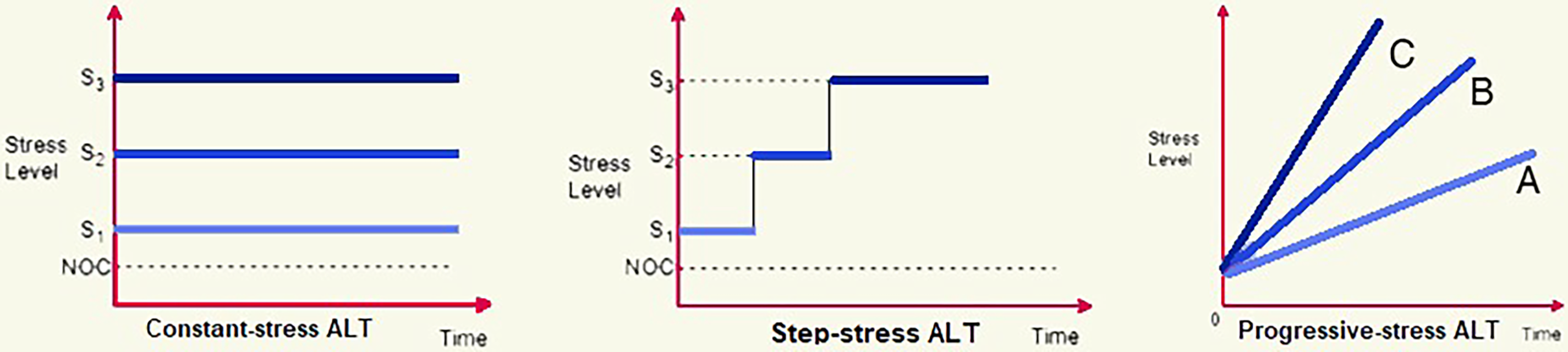
Figure 1: ALT types
Constant-stress ALT applies a fixed high stress until failure or a preset time, and has been widely used in reliability analysis. Several studies have proposed models and estimation techniques under this scheme, including works by Kumar et al. [2], Hakamipour [3], Balakrishnan et al. [4], Abd El-Raheem et al. [5], Sief et al. [6], El-Sherpieny et al. [7], and Abd El-Raheem et al. [8]. Step-stress ALT gradually increases stress at set intervals or after specific failures and is well established in reliability studies. Key contributions include works by Gouno et al. [9], Balakrishnan et al. [10], Xu et al. [11], Mohie El-Din [12], Xu et al. [13], Alotaibi et al. [14,15], and Hassan and Abdelghaffar [16], who developed various inference methods under different censoring and lifetime models.
Progressive-stress ALT elevates stress over time, unlike constant- and step-stress methods. The ramp-stress test, which increases tension linearly, is a common example. This method closely resembles real-world deterioration processes and is popular in dependability studies. For instance, Yin and Sheng [17] examined maximum likelihood estimation for exponential models under progressive stress. Bai and Cha [18] studied optimal test design and failure rate modeling under increasing load. Wang and Fei [19] studied statistical inference for Weibull distributions in modified failure rate models under increasing stress. Moreover, AL-Hussaini et al. [20] introduced Bayesian prediction ranges for the half-logistic distribution using Type-II censored data, demonstrating its versatility and effectiveness.
Censored data are commonly used in studies on reliability and life testing. Due to factors like preserving working experimental units for future use, reducing the overall time for the test, and financial limits, investigators have to gather data using censored samples. Time-censoring (Type-I) and failure-censoring (Type-II) strategies are the two widely used censoring strategies in life-testing and reliability studies (see, for additional details, the work by Bain and Engelhardt [21]). These methods are not flexible enough to allow units to be removed from the experiment at any point other than the terminal point.
The progressive Type-II censoring scheme (PTII) is a widely utilized method in reliability and survival analysis, often preferred over the standard Type-II censoring scheme due to its adaptability in practical applications such as industrial and medical studies. Unlike the conventional approach, PTII permits the removal of still-operational units during the experiment, rather than at its conclusion [22]. In PTII, suppose
To address this limitation, Kundu and Joarder [23] introduced the progressive hybrid censoring scheme (PHCS), where the test ends at
• Case I:
• Case II:
• Case III:
a schematic representation of the generalized progressive hybrid censoring scheme is presented in Fig. 2.
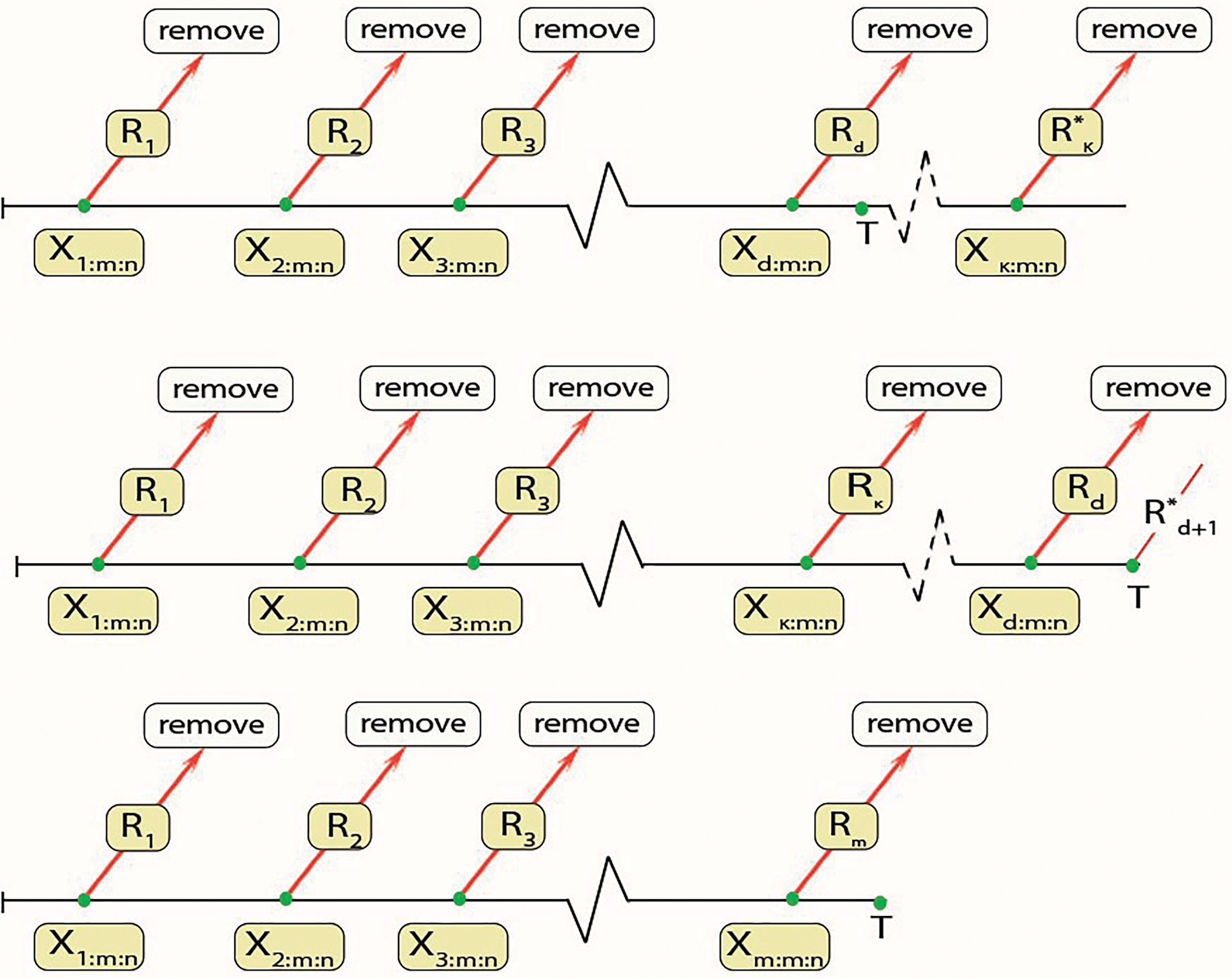
Figure 2: Diagram of GPHCS strategy
More paper used GPHCS for model a new dialog of censored sample as: Koley and Kundu [25] introduced GPHCS in the presence of competing risks models. Maswadah [26] improved maximum likelihood estimation of the shape-scale family based on GPHCS. Salem et al. [27] introduced joint Type-II of GPHCS. Abdelwahab et al. [28] discussed classical and Bayesian inference for lifetime distribution based on GPHCS. Mohie El-Din et al. [29] obtained predictions of lifetimes under GPHCS. Mahto et al. [30] developed a partially observed competing risk model under GPHSC. Zhu obtained reliability inference for the multi-component stress–strength model under GPHCS. Wang et al. [31] discussed the dependence of competing risks with partially observed failure causes from bivariate distribution under GPHCS. Çetinkaya [32] discussed inference of P (X > Y) under GPHCS. Shi et al. [33] introduced reliability analysis of the J-out-of-N system under GPHCS.
Research on progressive-stress ALT continues to expand, incorporating diverse statistical models and censoring schemes. Rong-hua and Heliang [19] applied it to Weibull distributions using tampered failure rate models. Abdel-Hamid and Al-Hussaini [34] combined progressive stress with finite mixture distributions, Bayesian analysis, and progressive censoring for various lifetime distributions. Abdel-Hamid and Al-Hussaini [35] also studied inference for Weibull distributions under PTII censoring. Recent works utilizing progressive-stress ALT with censoring schemes include studies by Mohie et al. [36], Zhuang et al. [37], Mahto et al. [38], Abushal and Abdel-Hamid [39], Ismail [40], Hussam et al. [41], and Alotaibi et al. [42].
The GPHC scheme has proven to be a valuable tool for analyzing censored data in ALTs, particularly in models like competing risks and step-stress models. However, a significant gap exists in the application of GPHC to Progressive Stress ALT models, which involve progressively increasing stress levels during the test. Most of the existing studies, such as those by Wang et al. [43] and Pandey et al. [44], focus on constant or step-stress models, without addressing the complexities introduced by progressive stress scenarios.
This paper extends the progressive-stress ALT framework by incorporating the QXG distribution—a flexible lifetime model suitable for diverse failure behaviors—under the GPHCS with binomial removal. To the best of our knowledge, this integration has not been addressed in the literature. The study contributes by:
• Developing classical and Bayesian estimation procedures for the QXG parameters under PSALT with GPHCS.
• Providing predictive survival probabilities under different censoring schemes.
• Conducting a thorough simulation to evaluate the performance of the estimators.
• Addressing a critical gap in the literature and paves the way for more realistic modeling of accelerated life tests.
• Demonstrating the methodology with real-world datasets.
This combination of modeling flexibility, advanced censoring, and estimation robustness aims to provide a more realistic and practically applicable framework for analyzing accelerated life test data.
The remainder of this paper is organized as follows: Section 2 presents the fundamental assumptions and details of the Quasi Xgamma distribution under the progressive-stress ALT model. Sections 3 and 4 describe the estimation methods, including both maximum likelihood and Bayesian approaches, respectively. Section 5 provides a comprehensive simulation study to assess the performance of the proposed estimators. Section 6 demonstrates the methodology using real-world accelerated life test datasets. Section 7 concludes the paper with final remarks and potential directions for future research.
The quasi xgamma distribution, introduced as a generalization of the xgamma distribution, adds flexibility in modeling lifetime data. Developed by Sen and Chandra [45], this distribution includes an additional parameter,
The cumulative distribution function (CDF) of the QXG distribution is given by:
The Quasi Xgamma (QXG) distribution was chosen for its flexibility in modeling lifetime data, especially under progressive-stress ALT. It includes a shape parameter
This model is quite versatile in nature and resembles probabilistic behavior in the gamma distribution and exponential distribution; see Sen and Chandra [45]. Recently, papers used QXG distribution as a baseline to obtain a new good distribution as: Sen et al. [46] discussed the QXG-geometric distribution with applications in medicine. Sen et al. [47] introduced QXG-Poisson distribution. Ahsan-ul-Haq et al. [48] discussed analysis, estimation, and practical implementations of the discrete power QXG distribution. Hassan et al. [49] obtained a new generalized QXG distribution applicable to survival times. Wani and Shafi [50] introduced the generalized Lindley-QXG distribution.
Assumption: Progressive-stress ALT
1. Lifetimes of units follow
2. We have stress function
3. The
4. We also have
5. Linear cumulative exposure model (LCEM) is considered for modeling the effect of stress change, for more details, see Nelson [1].
Under consideration of LCEM, the CDF under progressive-stress
where
Then by setting the value of the scale parameter
where
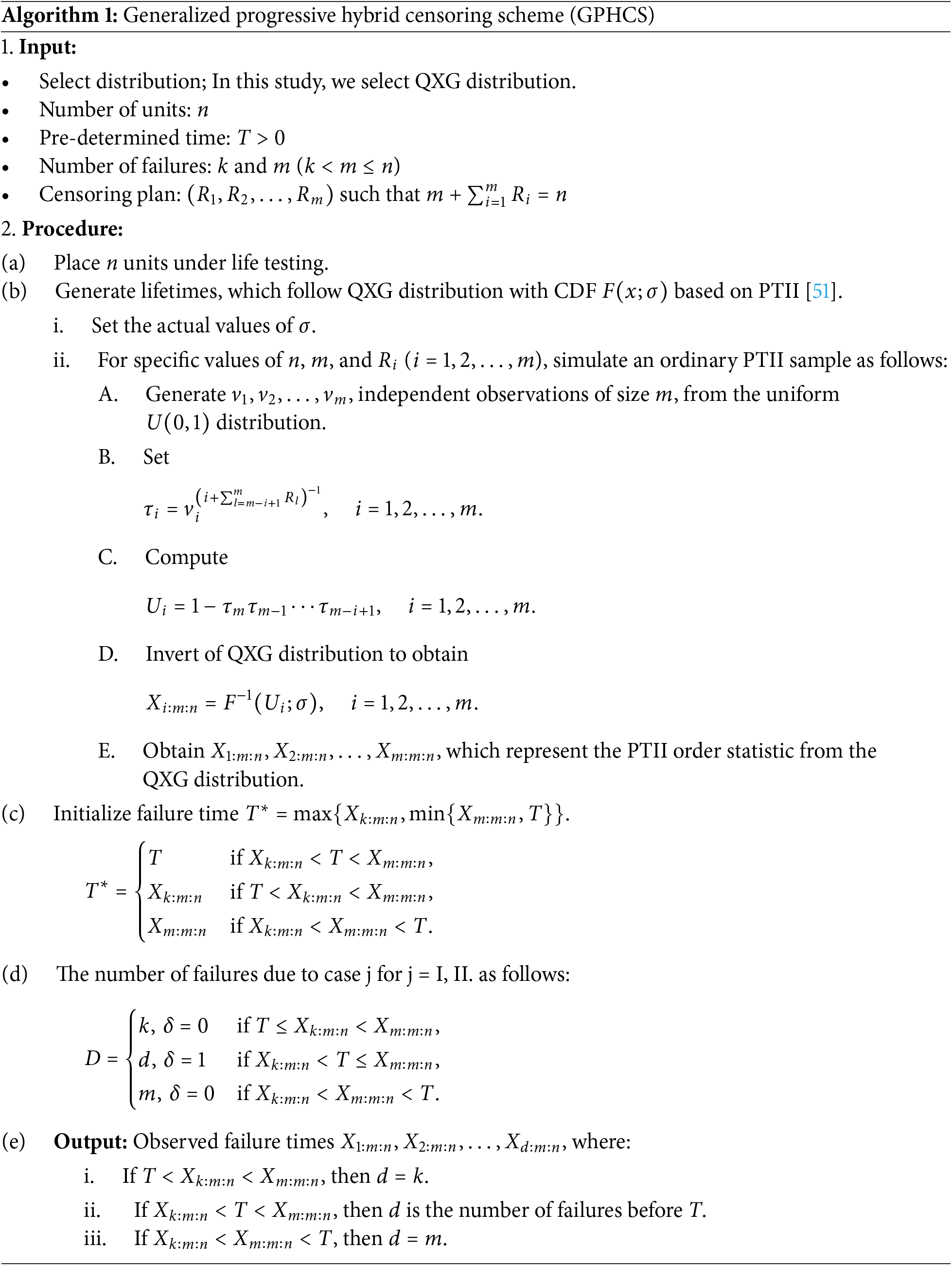
Algorithm 1 has been used To generate sample from generalized progressive hybrid censoring scheme.
In this section, we utilize the maximum likelihood estimation method based on PSALT to estimate the model parameters
During the first failure at the
Let the observed GPHCS data under the progressive-stress level
where
Using Eqs. (3) and (4) in (5), the likelihood function of the QXG distribution under GPHCS within the framework of the PSALT model is derived as:
hence, the log-likelihood function, excluding the constant term
The likelihood equations are obtained by taking the first partial derivatives of the log-likelihood function in (7) with respect to
and
where
The maximum likelihood estimates of the unknown parameters
Here,
3.2 Asymptotic Confidence Interval
In this subsection, approximate confidence intervals for the parameters are derived using the asymptotic distribution of the MLEs of
where
where
The following section explores the incorporation of prior knowledge into the analysis to achieve improved results.
In this section, Bayes estimates for the model parameters
where
The joint prior density function of
The mean and variance of the MLE for each of the
and
For more information about gamma prior, hyperparameters, and posterior distribution, see [53–56].
By combining Eqs. (11) and (6) and applying Bayes’ theorem, the joint posterior distribution is obtained as:
Deriving analytical Bayes estimators for the three parameters
The marginal posterior distribution of a parameter is derived by integrating the joint posterior distribution over the other parameter. Consequently, the marginal posterior probability density functions for
and
The Metropolis-Hastings (MH) algorithm is the preferred method for generating posterior samples to compute the desired Bayes estimates. This is because obtaining the conditional posterior distributions of the parameters
Steps of the Metropolis-Hastings algorithm:
1. Initialize the parameter values
2. Set the iteration index
3. Generate proposed values for the parameters as:
where
4. Calculate the acceptance ratio:
5. Accept the proposed values
6. Repeat steps (3) to (5) B times to generate B samples for the parameters
As described in [57], the Bayes estimators for the parameters
We remove first
The Bayes estimators for the parameters
4.2 Highest Posterior Density (HPD) Credible Interval
In this subsection, the HPD credible interval
Given the difficulty of determining the interval
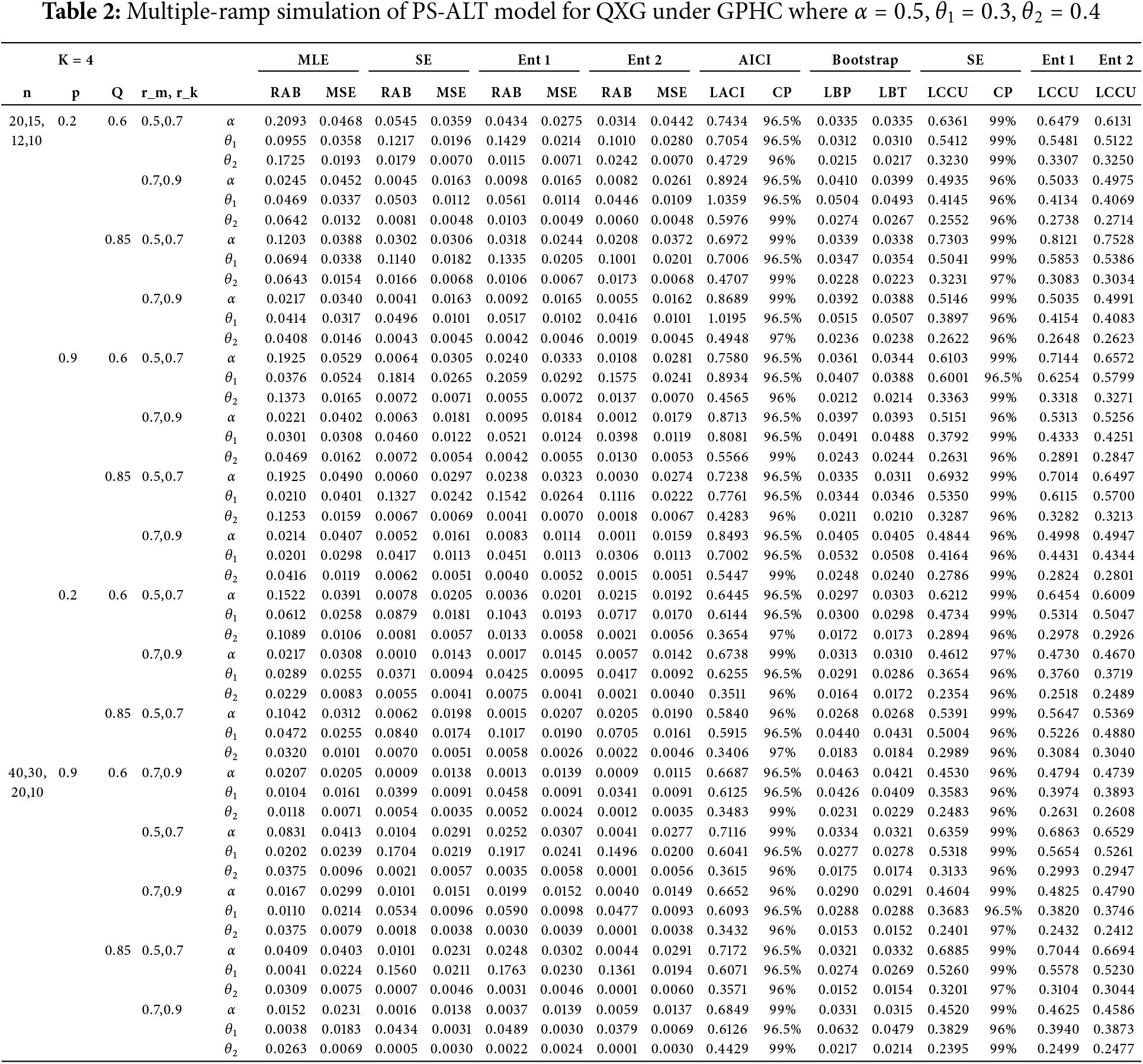
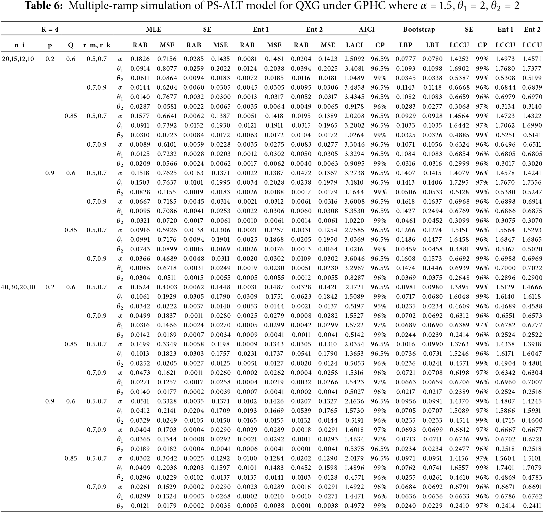
To evaluate the performance of the methods presented in this paper, a Monte Carlo simulation is carried out. The MLEs and Bayes estimates are compared based on their relative absolute bias (RAB), and mean squared errors (MSEs). Additionally, the asymptotic confidence intervals (ACI) and HPD intervals are assessed in terms of their average interval lengths and coverage probabilities. The simulation study involves three different progressive-stress accelerated life tests (ALTs): the first is a simple ramp-stress ALT with two stress levels (
and
where
Substituting (16) and (17) into (18), we get
In all scenarios considered, we have assumed
The true values of the parameters


The entire study is carried out for the first ramp-stress is Small sample:
The results shown in Tables 1–6 indicate that Bayes estimates of
Regarding the confidence intervals, Bayesian credible intervals for
For comparison, consider the censoring scheme using a binomial removal, where items are withdrawn immediately after the first failure, vs. predicted values for items withdrawn at the
To illustrate the proposed methodologies, we analyze an accelerated life test data set from [59,60].
First data set: The data presented in Chapter 5 of [59] were obtained from ramp-voltage tests conducted on miniature light bulbs designed to operate at a stress (voltage) of 2 V. In these tests, 62 miniature light bulbs were tested at a ramp rate of 2.01 V/h, while 61 bulbs were tested at a ramp rate of 2.015 V/h. The lifetime data from these ramp-voltage tests are provided by [36].
Second data includes failure times for the time-dependent dielectric breakdown of metal-oxide-semiconductor integrated circuits. The test was conducted at three elevated temperatures: 170°C, 200°C, and 250°C. For this study, we focus on the data collected at 170°C and 200°C.
To evaluate the suitability of the data for a QXG distribution, we calculate AIC, BIC, the Kolmogorov-Smirnov distance (KSD), and the corresponding p-values for each stress level. These results, along with the each data set, are presented in Tables 7 and 8, respectively. The QXG distribution is contrasted with four rival models, including the log-logistic (LogLog) [38], exponentiated Weibull (EW) [14], extended exponential (ExEx) distribution [36], and the logistic exponential (LogEx) distribution [61]. These models are evaluated using statistical measures such as AIC, BIC, KSD, and p-values.

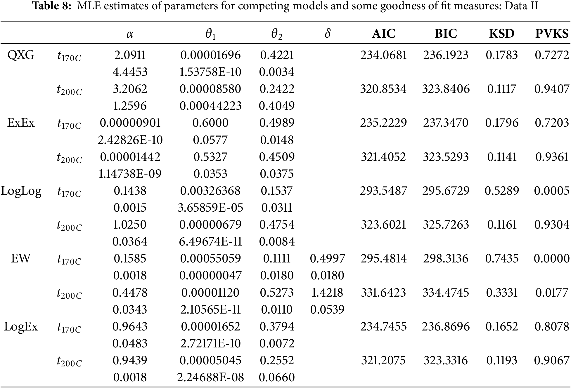
Tables 7 and 8 identify the best-fitting model as the one with the lowest AIC, BIC, and KSD values, combined with the highest p-values, indicating a superior fit to the QXG distribution.
Fig. 3 displays the likelihood profiles for the parameters
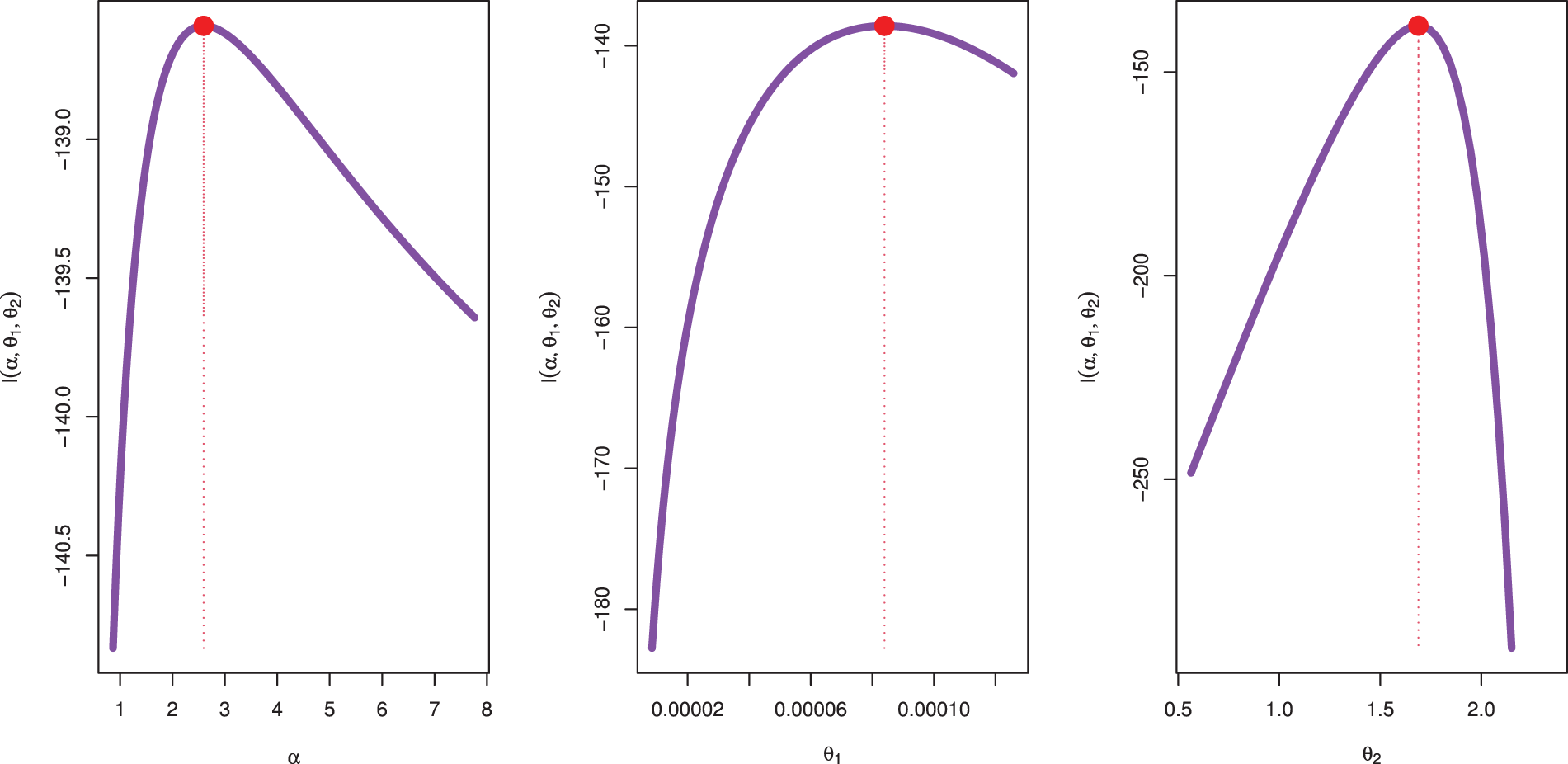
Figure 3: Likelihood profile for parameters of QXG based on PSALT with Data I
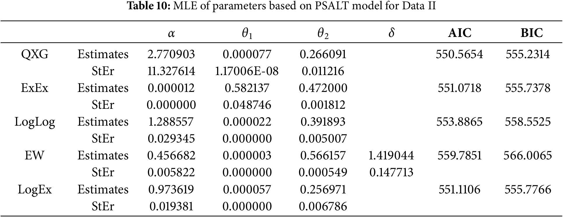
The results presented in Tables 9 and 10 summarize the MLE of parameters for various models under the PSALT framework, evaluated for two distinct datasets: Data I and Data II. The models compared include QXG, ExEx, LogLog, EW, and LogEx, with model performance assessed using the AIC and BIC. Lower values of AIC and BIC generally indicate better model fit for QXG under the PSALT model.
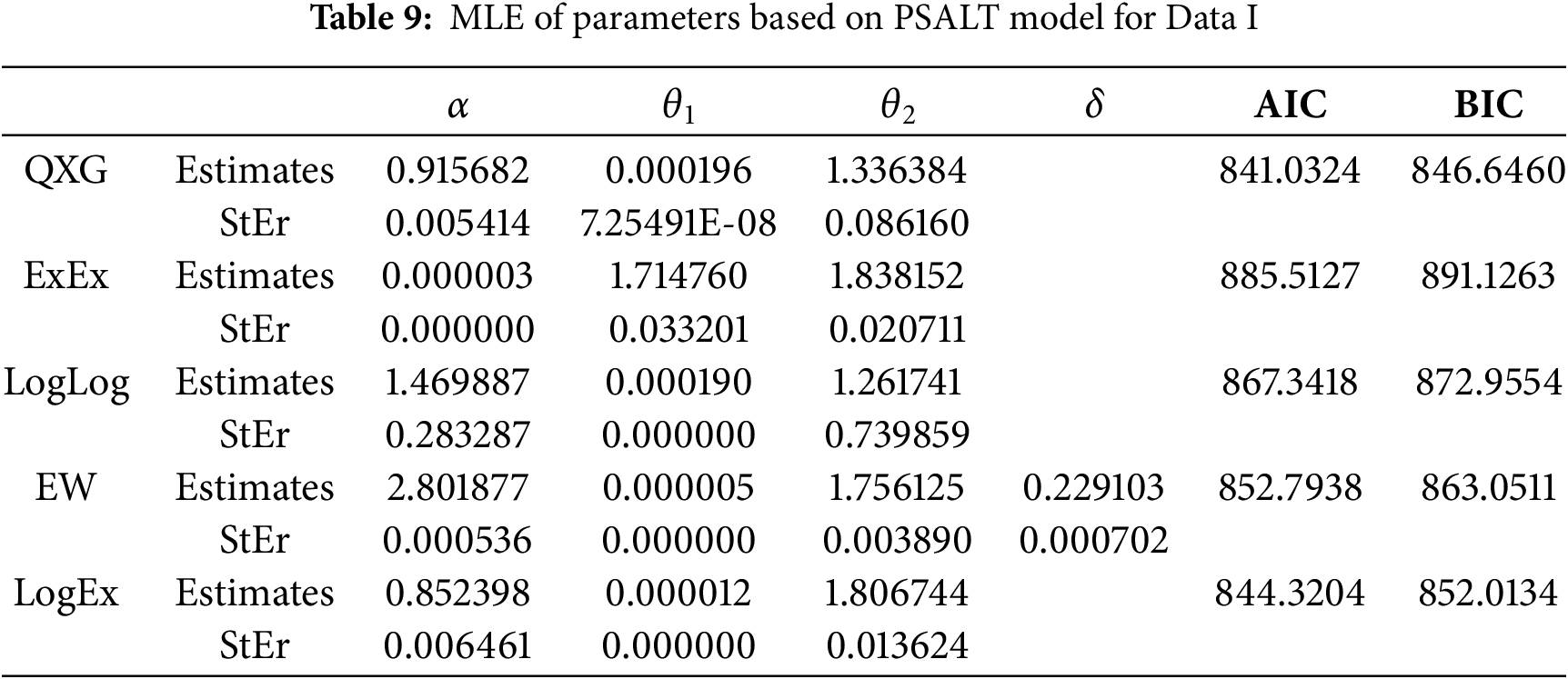
For Data I (Table 9), the QXG model emerges as the best-fitting model, with the lowest AIC (841.0324) and BIC (846.6460). The LogEx model performs competitively, but its AIC (844.3204) and BIC (852.0134) remain slightly higher than QXG. The ExEx model performs the worst, as evidenced by its significantly higher AIC (885.5127) and BIC (891.1263). The LogLog and EW models provide moderate fits, but neither outperforms QXG. Notably, the parameter estimates under QXG show relatively small standard errors, indicating precise and reliable estimates.
For Data II (Table 10), the QXG model again demonstrates superior performance, achieving the lowest AIC (550.5654) and BIC (555.2314). The ExEx and LogEx models follow closely, with AIC and BIC values that are only slightly higher, suggesting these models also offer reasonable fits for Data II. The EW model, despite its added parameter (
Table 11 presents progressively censored data for a specific dataset of amp-voltage tests conducted on miniature light bulbs designed to operate at a stress. The table shows different censoring schemes defined by

Figs. 4 and 5 show the MCMC diagnostic plots for the parameters
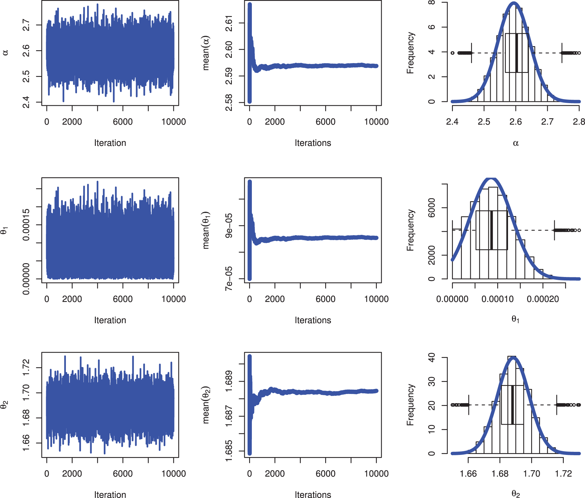
Figure 4: MCMC plots for parameters of QXG based on PSALT under GPHCS
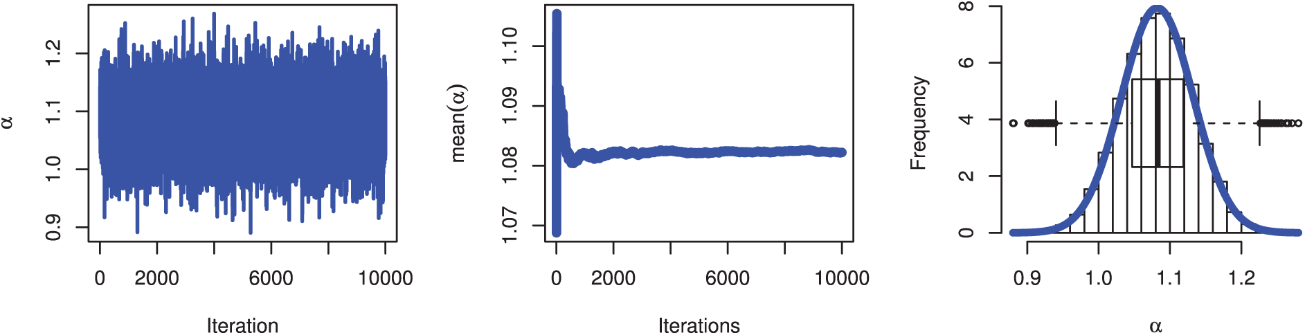
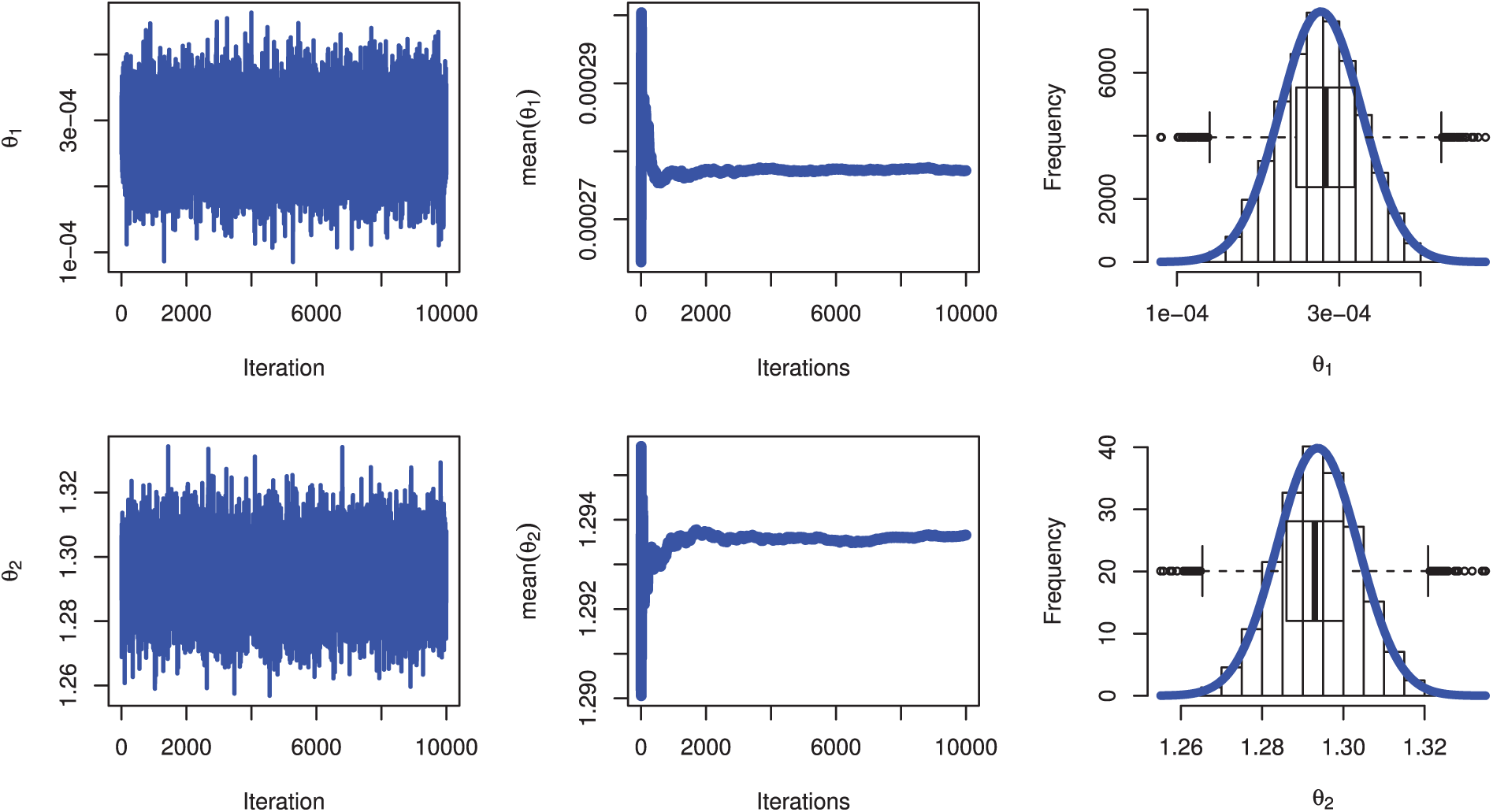
Figure 5: MCMC plots for parameters of QXG based on PSALT under GPHCS
Table 12 presented the results of parameter estimation for a dataset (Data I) under different stress levels, using both MLE and Bayesian methods with varying loss functions (SE, Ent 1, Ent 2). The table shows estimates for parameters

Fig. 6 illustrates the likelihood profiles for the parameters
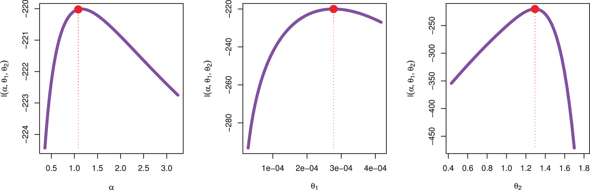
Figure 6: Likelihood profile for parameters of QXG based on PSALT under GPHCS
Table 13 presents progressively censored time-dependent dielectric breakdown of metal oxide-semiconductor integrated circuits data, temperatures 170°C and 200°C, censoring schemes, and their impact on statistical analysis. Table 14 discussed the results of parameter estimation for a dataset (Data II) under different stress levels
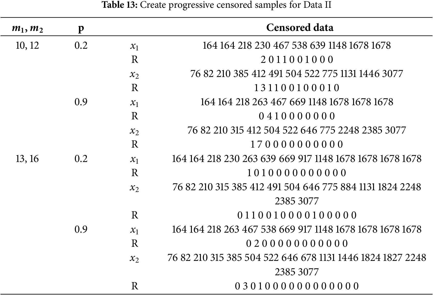
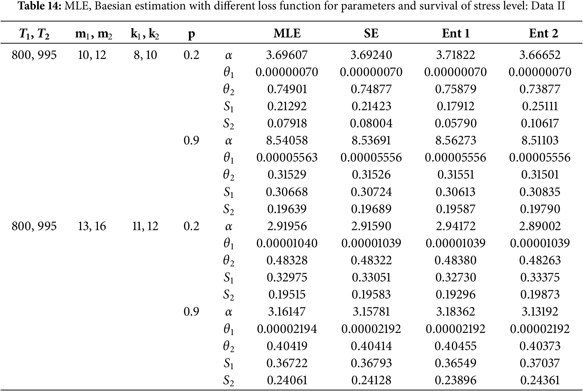
Tables 12 and 13 present the application of the proposed PSALT model under the Generalized Progressive Hybrid Censoring (GPHC) scheme to two distinct real-world datasets. These applications are intended to complement the simulation study by demonstrating the practical utility and flexibility of the proposed methodology. The analysis includes model fitting comparisons using criteria such as AIC, BIC, and KSD, confirming that the quasi Xgamma distribution under GPHC performs well relative to alternative models. These results provide empirical support for the robustness of the proposed approach in real-life accelerated life testing scenarios, as highlighted in the reviewer’s comment.
Figs. 7 and 8 present the likelihood profiles for the parameters
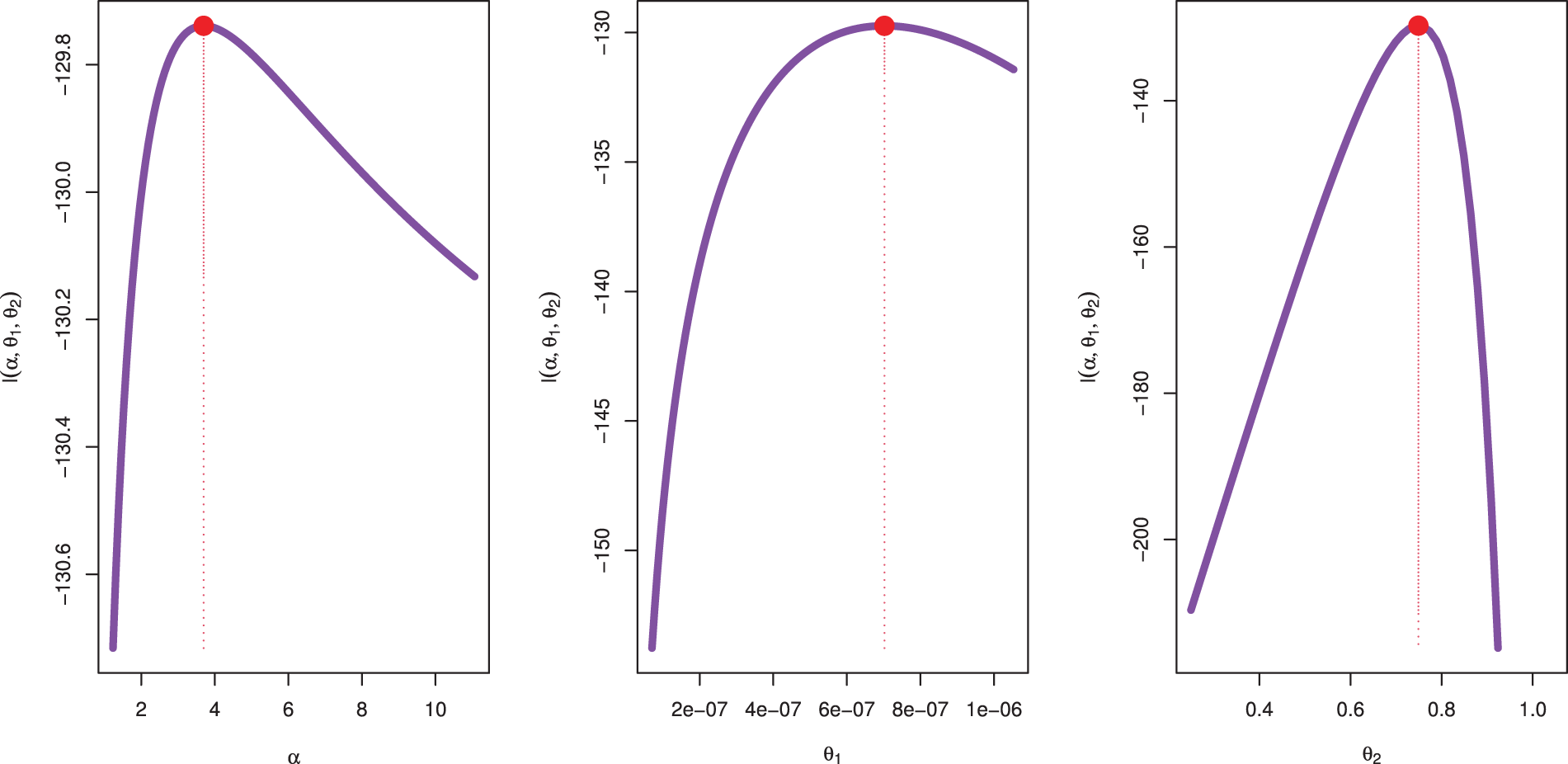
Figure 7: Likelihood profile for parameters of QXG based on PSALT under GPHCS

Figure 8: Likelihood profile for parameters of QXG based on PSALT under GPHCS
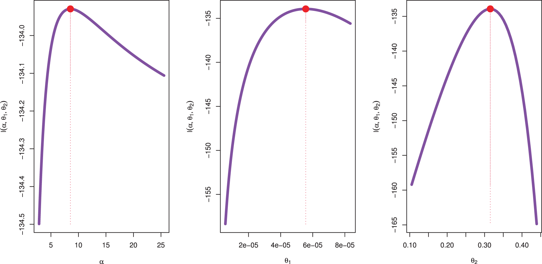
Figure 9: MCMC plots for parameters of QXG based on PSALT under GPHCS
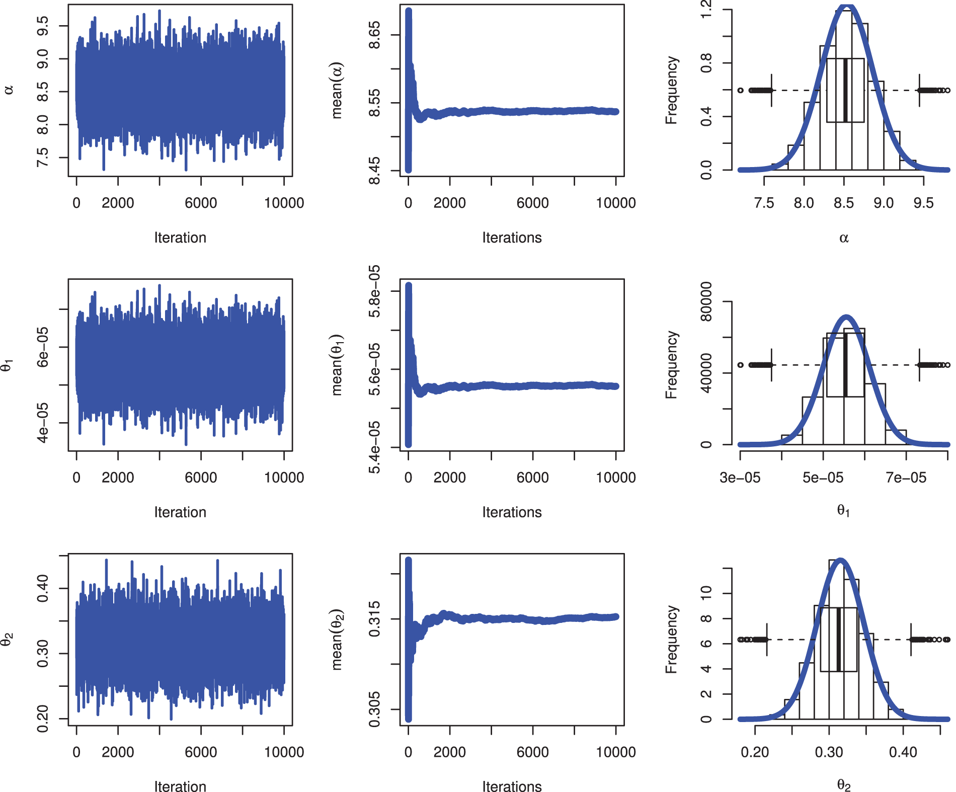
Figure 10: MCMC plots for parameters of QXG based on PSALT under GPHCS
This paper investigates progressive-stress ALT for the lifetime quasi xgamma distribution under a generalized progressive hybrid censoring scheme, demonstrating the proposed methods through a practical example. MLEs and Bayesian estimates of the parameters were derived for various sample sizes and two binomial parameter schemes for random removal, with their performance assessed through MSEs. Confidence intervals based on the asymptotic distribution of the MLEs were compared with those derived from posterior distributions. We constructed various confidence intervals, including asymptotic, boot-p, boot-t, and Bayesian intervals, within the PSALT framework. The simulation results suggest that Bayesian estimates generally outperform their classical counterparts, with p-boot intervals showing satisfactory coverage probabilities. The simulation study results indicate that Bayesian point estimates and HPD credible intervals outperform classical point estimates and confidence intervals with bootstrap. This trend was similarly reflected in two real-life data analyses. The QXG distribution based on progressive-stress ALT is compared to four competing models: log-logistic, exponentiated Weibull, extended exponential, and logistic exponential distributions based on progressive-stress ALT. The comparison, based on statistical measures such as AIC, BIC, KSD, and p-values, demonstrates that the QXG distribution based on progressive-stress ALT outperforms the rival models.
Acknowledgement: This work was supported and funded by the Deanship of Scientifc Research at Imam Mohammad Ibn Saud Islamic University (IMSIU) (grant number IMSIU-DDRSP2503).
Funding Statement: This work was supported and funded by the Deanship of Scientifc Research at Imam Mohammad Ibn Saud Islamic University (IMSIU) (grant number IMSIU-DDRSP2503).
Author Contributions: The authors confirm contribution to the paper as follows: Conceptualization, Ehab M. Almetwally and O. M. Khaled; methodology, Ehab M. Almetwally and H. M. Barakat; software, Ehab M. Almetwally; validation, O. M. Khaled, H. M. Barakat and Ehab M. Almetwally; formal analysis, O. M. Khaled; investigation, H. M. Barakat; resources, Ehab M. Almetwally; data curation, Ehab M. Almetwally; writing—original draft preparation, Ehab M. Almetwally; writing—review and editing, Ehab M. Almetwally, O. M. Khaled and H. M. Barakat; visualization, H. M. Barakat; supervision, H. M. Barakat; project administration, H. M. Barakat; funding acquisition, Ehab M. Almetwally. All authors reviewed the results and approved the final version of the manuscript.
Availability of Data and Materials: All data generated or analyzed during this study are included in this published article.
Ethics Approval: Not applicable.
Conflicts of Interest: The authors declare no conflicts of interest to report regarding the present study.
References
1. Nelson WB. Accelerated testing: statistical models, test plans, and data analysis. Hoboken, NJ, USA: John Wiley & Sons; 2009. [Google Scholar]
2. Kumar D, Nassar M, Dey S, Alam FMA. On estimation procedures of constant stress accelerated life test for generalized inverse Lindley distribution. Qual Reliab Eng Int. 2022;38(1):211–28. doi:10.1002/qre.2971. [Google Scholar] [CrossRef]
3. Hakamipour N. Parameter estimation using EM algorithm and test design optimization of constant stress accelerated life test with non-constant parameters under type-I progressive censoring. J Decis Oper Res. 2022;6(4):570–91. doi:10.22105/DMOR.2021.287322.1405. [Google Scholar] [CrossRef]
4. Balakrishnan N, Castilla E, Ling MH. Optimal designs of constant-stress accelerated life-tests for one-shot devices with model misspecification analysis. Qual Reliab Eng Int. 2022;38(2):989–1012. doi:10.1002/qre.3031. [Google Scholar] [CrossRef]
5. Abd El-Raheem AM, Abu-Moussa MH, Mohie El-Din MM, Hafez EH. Accelerated life tests under Pareto-IV lifetime distribution: real data application and simulation study. Mathematics. 2020;8(10):1786. doi:10.3390/math8101786. [Google Scholar] [CrossRef]
6. Sief M, Liu X, Hosny M, Abd El-Raheem AERM. Constant-stress modeling of log-normal data under progressive type-I interval censoring: maximum likelihood and bayesian estimation approaches. Axioms. 2023;12(7):710. doi:10.3390/axioms12070710. [Google Scholar] [CrossRef]
7. El-Sherpieny ESA, Muhammed HZ, Almetwally EM. Accelerated life-testing for bivariate distributions based on progressive censored samples with random removal. J Stat Appl Probab. 2022;11(2):203–23. [Google Scholar]
8. Abd El-Raheem AM, Almetwally EM, Mohamed MS, Hafez EH. Accelerated life tests for modified Kies exponential lifetime distribution: binomial removal, transformers turn insulation application and numerical results. AIMS Math. 2021;6(5):5222–55. doi:10.3934/math.2021310. [Google Scholar] [CrossRef]
9. Gouno E, Sen A, Balakrishnan N. Optimal step-stress test under progressive Type-I censoring. IEEE Trans Reliab. 2004;53(3):388–93. doi:10.1109/tr.2004.833320. [Google Scholar] [CrossRef]
10. Balakrishnan N, Kundu D, Ng KT, Kannan N. Point and interval estimation for a simple step-stress model with Type-II censoring. J Qual Technol. 2007;39(1):35–47. doi:10.1080/00224065.2007.11917671. [Google Scholar] [CrossRef]
11. Xu A, Fang G, Zhuang L, Gu C. A multivariate student-t process model for dependent tail-weighted degradation data. IISE Trans. 2024;57(9):1071–87. doi:10.1080/24725854.2024.2389538. [Google Scholar] [CrossRef]
12. Mohie El-Din MM, Abd El-Raheem AM, Abd El-Azeem SO. On step-stress accelerated life-testing for power generalized Weibull distribution under progressive type-II censoring. Ann Data Sci. 2021;8(3):629–44. doi:10.1007/s40745-020-00270-4. [Google Scholar] [CrossRef]
13. Xu A, Wang R, Weng X, Wu Q, Zhuang L. Strategic integration of adaptive sampling and ensemble techniques in federated learning for aircraft engine remaining useful life prediction. Appl Soft Comput. 2025;175(6):113067. doi:10.1016/j.asoc.2025.113067. [Google Scholar] [CrossRef]
14. Alotaibi N, Elbatal I, Almetwally EM, Alyami SA, Al-Moisheer AS, Elgarhy M. Bivariate step-stress accelerated life tests for the Kavya-Manoharan exponentiated Weibull model under progressive censoring with applications. Symmetry. 2022;14(9):1791. doi:10.3390/sym14091791. [Google Scholar] [CrossRef]
15. Alotaibi R, Almetwally EM, Ghosh I, Rezk H. Statistical inference of a step-stress model with competing risks under time censoring for alpha power exponential distribution. J Radiat Res Appl Sci. 2024;17(1):100771. doi:10.1016/j.jrras.2023.100771. [Google Scholar] [CrossRef]
16. Hassan AS, Abdelghaffar AM. Bayesian and E-Bayesian estimation of gompertz distribution in stress-strength reliability model under partially accelerated life testing. Comput J Math Stat Sci. 2025;4(1):348–78. doi:10.21608/cjmss.2025.353923.1107. [Google Scholar] [CrossRef]
17. Yin XK, Sheng BZ. Some aspects of accelerated life-testing by progressive stress. IEEE Trans Reliab. 1987;36(1):150–5. doi:10.1109/tr.1987.5222320. [Google Scholar] [CrossRef]
18. Bai DS, Cha MS, Chung SW. Optimum simple ramp-tests for the Weibull distribution and type-I censoring. IEEE Trans Reliab. 1992;41(3):407–13. doi:10.1109/24.159808. [Google Scholar] [CrossRef]
19. Wang RH, Fei H. Statistical inference of Weibull distribution for tampered failure rate model in progressive stress accelerated life-testing. J Syst Sci Complex. 2004;14(2):237–43. doi:10.1520/jte20130115. [Google Scholar] [CrossRef]
20. AL-Hussaini EK, Abdel-Hamid AH, Hashem AF. One-sample Bayesian prediction intervals based on progressively type-II censored data from the half-logistic distribution under progressive stress model. Metrika. 2015;78(6):771–83. doi:10.1007/s00184-014-0526-4. [Google Scholar] [CrossRef]
21. Engelhardt M, Bain LJ. Some results on point estimation for the two-parameter Weibull or extreme-value distribution. Technometrics. 1974;16(1):49–56. doi:10.1080/00401706.1974.10489148. [Google Scholar] [CrossRef]
22. Balakrishnan N, Aggarwala R. Progressive censoring: theory, methods, and applications. New York, NY, USA: Springer Science & Business Media; 2000. [Google Scholar]
23. Kundu D, Joarder A. Analysis of Type-II progressively hybrid censored data. Comput Stat Data Anal. 2006;50(10):2509–28. doi:10.1016/j.csda.2005.05.002. [Google Scholar] [CrossRef]
24. Cho Y, Sun H, Lee K. Exact likelihood inference for an exponential parameter under generalized progressive hybrid censoring scheme. Stat Methodol. 2015;23:18–34. doi:10.1016/j.stamet.2014.09.002. [Google Scholar] [CrossRef]
25. Koley A, Kundu D. On generalized progressive hybrid censoring in presence of competing risks. Metrika. 2017;80(3):401–26. doi:10.1007/s00184-017-0611-6. [Google Scholar] [CrossRef]
26. Maswadah M. Improved maximum likelihood estimation of the shape-scale family based on the generalized progressive hybrid censoring scheme. J Appl Stat. 2022;49(11):2825–44. doi:10.1080/02664763.2021.1924638. [Google Scholar] [CrossRef]
27. Salem S, Abo-Kasem OE, Hussien A. On joint Type-II generalized progressive hybrid censoring scheme. Comput J Math Stat Sci. 2023;2(1):123–58. doi:10.21608/cjmss.2023.193844.1004. [Google Scholar] [CrossRef]
28. Abdelwahab MM, Ghorbal AB, Hassan AS, Elgarhy M, Almetwally EM, Hashem AF. Classical and Bayesian inference for the Kavya-Manoharan generalized exponential distribution under generalized progressively hybrid censored data. Symmetry. 2023;15(6):1193. doi:10.3390/sym15061193. [Google Scholar] [CrossRef]
29. Mohie El-Din MM, Nagy M, Abu-Moussa MH. Estimation and prediction for Gompertz distribution under the generalized progressive hybrid censored data. Ann Data Sci. 2019;6(4):673–705. doi:10.1007/s40745-019-00199-3. [Google Scholar] [CrossRef]
30. Mahto AK, Lodhi C, Tripathi YM, Wang L. On partially observed competing risk model under generalized progressive hybrid censoring for Lomax distribution. Qual Technol Quant Manag. 2022;19(5):562–86. doi:10.1080/16843703.2022.2049507. [Google Scholar] [CrossRef]
31. Wang L, Tripathi YM, Dey S, Shi Y. Inference for dependence competing risks with partially observed failure causes from bivariate Gompertz distribution under generalized progressive hybrid censoring. Qual Reliab Eng Int. 2021;37(3):1150–72. doi:10.1002/qre.2787. [Google Scholar] [CrossRef]
32. Çetinkaya Ç. Inference of P (X > Y) for the Burr-XII model under generalized progressive hybrid censored data with binomial removals. Concurr Comput Pract Exp. 2023;35(7):e7609. doi:10.1002/cpe.7609. [Google Scholar] [CrossRef]
33. Shi X, Shi Y, Song Q. Reliability analysis of J-out-of-N system with Nadarajah-Haghighi component under generalised progressive hybrid censoring. Int J Syst Sci. 2022;53(7):1436–55. doi:10.1080/00207721.2021.2005176. [Google Scholar] [CrossRef]
34. Abdel-Hamid AH, Al-Hussaini EK. Progressive stress accelerated life tests under finite mixture models. Metrika. 2007;66(3):213–31. doi:10.1007/s00184-006-0106-3. [Google Scholar] [CrossRef]
35. Abdel-Hamid AH, Al-Hussaini EK. Inference for a progressive stress model from Weibull distribution under progressive type-II censoring. J Comput Appl Math. 2011;235(17):5259–71. doi:10.1016/j.cam.2011.05.035. [Google Scholar] [CrossRef]
36. Mohie El-Din MM, Abu-Youssef SE, Ali NS, Abd El-Raheem AM. Classical and Bayesian inference on progressive-stress accelerated life-testing for the extension of the exponential distribution under progressive type-II censoring. Qual Reliab Eng Int. 2017;33(8):2483–96. doi:10.1002/qre.2212. [Google Scholar] [CrossRef]
37. Zhuang L, Xu A, Wang B, Xue Y, Zhang S. Data analysis of progressive-stress accelerated life tests with group effects. Qual Technol Quant Manag. 2023;20(6):763–83. doi:10.1080/16843703.2022.2147690. [Google Scholar] [CrossRef]
38. Mahto AK, Tripathi YM, Dey S, Alsaedi BS, Alhelali MH, Alghamdi FM, et al. Bayesian estimation and prediction under progressive-stress accelerated life test for a log-logistic model. Alex Eng J. 2024;101(02):330–42. doi:10.1016/j.aej.2024.05.045. [Google Scholar] [CrossRef]
39. Abushal TA, Abdel-Hamid AH. Inference on a new distribution under progressive-stress accelerated life tests and progressive type-II censoring based on a series-parallel system. AIMS Math. 2022;7(1):425–54. doi:10.3934/math.2022028. [Google Scholar] [CrossRef]
40. Ismail AA. Progressive stress accelerated life test for inverse Weibull failure model: a parametric inference. J King Saud Univ Sci. 2022;34(4):101994. doi:10.1016/j.jksus.2022.101994. [Google Scholar] [CrossRef]
41. Hussam E, Alharbi R, Almetwally EM, Alruwaili B, Gemeay AM, Riad FH. Single and multiple ramp progressive stress with binomial removal: practical application for industry. Math Probl Eng. 2022;2022(3):9558650. doi:10.1155/2022/9558650. [Google Scholar] [CrossRef]
42. Alotaibi R, Alamri FS, Almetwally EM, Wang M, Rezk H. Classical and bayesian inference of a progressive-stress model for the Nadarajah-Haghighi distribution with type II progressive censoring and different loss functions. Mathematics. 2022;10(9):1602. doi:10.3390/math10091602. [Google Scholar] [CrossRef]
43. Wang L, Tripathi YM, Lodhi C, Zuo X. Inference for constant-stress Weibull competing risks model under generalized progressive hybrid censoring. Math Comput Simul. 2022;192(4):70–83. doi:10.1016/j.matcom.2021.08.017. [Google Scholar] [CrossRef]
44. Pandey A, Kaushik A, Singh SK, Singh U. Statistical analysis for generalized progressive hybrid censored data from Lindley distribution under step-stress partially accelerated life test model. Austrian J Stat. 2021;50(1):105–20. doi:10.17713/ajs.v50i1.1004. [Google Scholar] [CrossRef]
45. Sen S, Chandra N. The quasi xgamma distribution with application in bladder cancer data. J Data Sci. 2017;15(1):61–76. doi:10.6339/JDS.201701_15(1).0004. [Google Scholar] [CrossRef]
46. Sen S, Afify AZ, Al-Mofleh H, Ahsanullah M. The quasi xgamma-geometric distribution with application in medicine. Filomat. 2019;33(16):5291–330. doi:10.2298/FIL1916291S. [Google Scholar] [CrossRef]
47. Sen S, Korkmaz MÇ., Yousof HM. The quasi XGamma-Poisson distribution: properties and application. Istatistik J Turk Stat Assoc. 2018;11(3):65–76. [Google Scholar]
48. Ahsan-ul-Haq M, Hussain MNS, Babar A, Al-Essa LA, Eliwa MS, Martinucci B. Analysis, estimation, and practical implementations of the discrete power quasi‐xgamma distribution. J Math. 2024;2024(1):1913285. doi:10.1155/2024/1913285. [Google Scholar] [CrossRef]
49. Hassan A, Wani SA, Ahmad SB, Akhtar N. A new generalized quasi Xgamma distribution applicable to survival times. J Xi’an Univ Archit Technol. 2020;12(4):3720–36. [Google Scholar]
50. Wani SA, Shafi S. Generalized Lindley-Quasi Xgamma distribution. J Appl Math Stat Inform. 2021;17(1):5–30. doi:10.2478/jamsi-2021-0001. [Google Scholar] [CrossRef]
51. Balakrishnan N, Sandhu RA. A simple simulational algorithm for generating progressive Type-II censored samples. Am Stat. 1995;49(2):229–30. doi:10.1080/00031305.1995.10476150. [Google Scholar] [CrossRef]
52. Dey S, Dey T, Luckett DJ. Statistical inference for the generalized inverted exponential distribution based on upper record values. Math Comput Simul. 2016;120(11):64–78. doi:10.1016/j.matcom.2015.06.012. [Google Scholar] [CrossRef]
53. Alotaibi N, Al-Moisheer AS, Elbatal I, Elgarhy M, Almetwally EM. Bayesian and non-bayesian analysis for the sine generalized linear exponential model under progressively censored data. Comput Model Eng Sci. 2024;140(3):2795–823. doi:10.32604/cmes.2024.049188. [Google Scholar] [CrossRef]
54. Abdelall YY, Hassan AS, Almetwally EM. A new extention of the odd inverse Weibull-G family of distributions: bayesian and non-Bayesian estimation with engineering applications. Comput J Math Stat Sci. 2024;3(2):359–88. doi:10.21608/cjmss.2024.285399.1050. [Google Scholar] [CrossRef]
55. Mohamed AA, Refaey RM, AL-Dayian GR. Bayesian and E-Bayesian estimation for odd generalized exponential inverted Weibull distribution. J Bus Environ Sci. 2024;3(2):275–301. doi:10.21608/jcese.2024.288853.1061. [Google Scholar] [CrossRef]
56. Alotaibi R, Nassar M, Elshahhat A. Computational analysis of novel extended lindley progressively censored data. Comput Model Eng Sci. 2024;138(3):2571–96. doi:10.32604/cmes.2023.030582. [Google Scholar] [CrossRef]
57. Calabria R, Pulcini G. Point estimation under asymmetric loss functions for left-truncated exponential samples. Commun Stat Theory Methods. 1996;25(3):585–600. doi:10.1080/03610929608831715. [Google Scholar] [CrossRef]
58. Chen MH, Shao QM. Monte Carlo estimation of Bayesian credible and HPD intervals. J Comput Graph Stat. 1999;8(1):69–92. doi:10.1080/10618600.1999.10474802. [Google Scholar] [CrossRef]
59. Zhu Y. Optimal design and equivalency of accelerated life testing plans [dissertation]. New Brunswick, NJ, USA: The State University of New Jersey; 2010. [Google Scholar]
60. Pham H. Recent studies in software reliability engineering. In: Handbook of reliability engineering. London, UK: Springer; 2003. p. 285–302 doi: 10.1007/1-85233-841-5_16. [Google Scholar] [CrossRef]
61. Kumar Mahto A, Dey S, Mani Tripathi Y. Statistical inference on progressive-stress accelerated life testing for the logistic exponential distribution under progressive type-II censoring. Qual Reliab Eng Int. 2020;36(1):112–24. doi:10.1002/qre.2562. [Google Scholar] [CrossRef]
Cite This Article
 Copyright © 2025 The Author(s). Published by Tech Science Press.
This work is licensed under a Creative Commons Attribution 4.0 International License , which permits unrestricted use, distribution, and reproduction in any medium, provided the original work is properly cited.
 Downloads
 Citation Tools