Systematic Benchmarking of Topology Optimization Methods Using Both Binary and Relaxed Forms of the Zhou-Rozvany Problem

1  Introduction

Topology optimization, as a conceptual design tool, has been widely applied in the fields of aerospace, automotive manufacturing, and biomedical science [1–3]. Common element-based topology optimization methods typically determine the optimal material distribution by solving problems in either their binary or relaxed form. In the binary form of topology optimization, the material distribution within the design domain is represented by only two values, 0 and 1, indicating void and solid regions, respectively. Methods belonging to this category include the Evolutionary Structural Optimization (ESO) [4] and the Bidirectional Evolutionary Structural Optimization (BESO) [5,6]. In contrast, the relaxed form allows the material density in each element of the design domain to vary continuously between 0 and 1, which introduces intermediate values that must be pushed back to the binary limits using a regularization technique. The Solid Isotropic Material with Penalization (SIMP) method [7] is an example of this approach.

The importance of having standard benchmarks to evaluate the performance of different proposed methods has been recognized in topology optimization [8]. A number of problems, like the simply supported MBB (Messerschmitt-Bölkow-Blohm) beam, have been used as classic benchmarks to test topology optimization methods [9]. However, apart from few limited cases [10–12], the benchmark problems used have no exact solution. Very few computational and theoretical results on global optimization using deterministic methods are available for the topology optimization of continuum structures [13], and such results are even more scarce for multiphysics and multimaterial problems [14–16]. One of the problems with relatively few design variables for which global optimal solutions are known is the Zhou-Rozvany (ZR) problem [17].

The ZR problem is originally introduced to illustrate the limitations of the ESO method in solving topology optimization problems [18]. It involves optimizing a tie beam demonstrated in Fig. 1. The structure is supported by a fixed boundary condition on the left side and a roller support at the top. The material is modeled as linearly elastic and isotropic, with a Young’s modulus of 1.0 and a Poisson’s ratio of 0.3. The loading conditions consist of a horizontal force with an intensity of 2.0 and a vertical force with an intensity of 1.0. The design domain is discretized using 100 four-node quadrilateral elements.

Figure 1: Geometry and boundary conditions for the ZR problem

Using ESO on this problem results in Fig. 2 where the tie breaks and the optimization method fails to recover it and successfully solve the problem. Rozvany stated that the issue observed in ESO cannot be solved by using its bidirectional version, BESO [18].

Figure 2: The solution obtained by ESO for the ZR problem after removing 1 element

Due to the significance of the ZR problem in evaluating binary-based topology optimization methods, Several research works investigated the reasons why binary methods like ESO and BESO fail to solve the ZR problem and proposed different approaches to address this issue. Some of the suggested techniques include mesh refinement [19,20], using soft elements [21], and freezing elements [4]. Rozvany [22] critically reviewed and questioned most of these suggestions. Ghabraie [23] showed that using high-order sensitivity analysis can help binary-based methods like ESO solve the ZR problem but highlighted that ESO also suffers from its unidirectional approach to the solution. More recently, the ZR problem is solved by adding a connectivity constraint into the BESO method [24].

The ZR problem is suggested to be introduced into the standard repertoire of benchmark examples when assessing new topology optimization methods [17]. To facilitate this benchmarking, Stolpe and Bendsøe [17] provided the global optima for the binary formulation of the ZR problem across different volume constraints. However, most of the material distribution-based topology optimization methods convert the binary form to a continuous form before solving it and then push the solution back to binary limits. The binary form of the ZR problem cannot be used to benchmark these methods properly, because as emphasized by Sigmund et al. [25], the selected form of the problem can have a great impact on the final solution. To properly benchmark topology optimization methods that solve the relaxed form of the problem, it would be ideal to consider solutions to both relaxed and binary forms of the benchmark problem.

To establish the ZR problem as a comprehensive benchmark, this study utilizes both its global binary solution [17] and its relaxed (convex) global solution, obtained via the Variable Thickness Sheet (VTS) formulation [25]. This work implements a grayness measure (based on the proposed measure of discreteness in [26]) to systematically benchmark a selected list of topology optimization methods against both binary and relaxed global optima of the ZR problem. Selected topology optimization methods include SIMP with a penalty factor of 3.0, SIMP combined with a continuation method [27], and the recently developed non-penalization Smooth-edged Material Distribution for Optimizing Topology (SEMDOT) method [28,29]. It should be noted that SEMDOT involves two steps: 1) solving the relaxed form and pushing it to binary using the Heaviside smooth function resulting in greyscale solutions, and 2) finding the smooth boundary of the design using a bisection approach on grid point densities. While the results obtained after the first step of SEMDOT should be benchmarked against both relaxed and binary solutions, its final smooth results can be benchmarked against the binary solutions.

The rest of this paper is organized as follows: Section 2 summarizes the global solutions to the relaxed and binary forms of the ZR problem. Section 3 proposes an indicator to measure the relaxedness of solutions. Section 4 explains the topology optimization methods to be benchmarked. Section 5 benchmarks the SIMP, SIMP with continuation, and grayscale SEMDOT results, discussing their Pareto fronts. Section 7 evaluates the smooth structures from the SEMDOT method more accurately by remeshing approach, presenting the Pareto front for binary-form designs. Finally, conclusions are drawn in Section 8.

2  Global Solutions for Binary and Relaxed Forms of the ZR Problem

Binary and relaxed forms of the ZR problem can be formulated as:

minx⁡C(xe)=fTusubjectto:K(xe)u=fand∑e=1100xe100−V∗≤0xe∈[0,1]forrelaxedformxe∈{0,1}forbinaryform(1)

where x=[x1,x2,…,x100] is the vector of design variables, C(xe) is the objective function of mean compliance; K(xe) is the stiffness matrix which depends on design variables; f is the nodal load vector; u is the nodal displacement vector, and V∗ is the target design volume fraction. xe is the design variable of element e and will vary continuously between 0 and 1 if the relaxed form is used, or it could only be 0 or 1 in the binary form.

For plane stress problems, the relaxed version of Eq. (1) is a convex VTS problem [7,25,30]. The VTS problem can be solved by using SIMP with a penalty factor of 1 (no penalization) and the solutions obtained will be global as the problem is convex. The global optima for the binary form are presented in [17]. These two sets of global optima are shown in Fig. 3.

Figure 3: Optimal Pareto fronts for both relaxed and binary forms of ZR problem [17]

As expected, the solutions of the relaxed form are always lower than those of the binary form. This is because the binary form is much more restrictive. Note that, unlike the relaxed form, the binary form cannot be solved at very low-volume fractions. Hence the Pareto fronts in Fig. 3 are presented for V∗≤0.4. The optimal solutions of both forms at the volume fraction of 0.4 are shown in Fig. 4 for comparison.

Figure 4: Optimal designs at V∗=0.4 for binary (a) and relaxed (b) forms of the ZR problem

3  Measuring the Relaxedness of a Solution

To assess the relaxedness of a solution, a grayness measure defined below is used in this study:

g(x)=1N∑e=1N(xe)⋅(1−xe)(2)

where N is the number of design variables in the design domain, commonly defined as 100 for the original ZR problem. The grayness value for a single element will be 0 if that element is either solid (xe=1) or void (xe=0), and a positive value for all intermediate values. Larger g values indicate greater deviation from a binary design, typically observed in more relaxed solutions, while smaller values suggest closer proximity to a binary form. This measure is proportional to the measure of discreteness (Mnd) defined in [26], with g=Mnd/4. It should also be noted that the number of elements N in the ZR problem is fixed at 100. To facilitate a more intuitive comparison of the grayness values, the fixed denominator N is omitted in the calculation.

The VTS formulation represents a fully relaxed formulation in topology optimisation, making the problem fully convex and resulting in density fields that significantly deviate from binary designs. Therefore, the maximum grayness value, denoted by g¯, is expected to be achieved by the results obtained from the VTS method, as shown along the VTS Pareto front in Fig. 3. The values of g¯≡g¯(V∗) are reported in Table 1. The binary solutions have the g value of 0. For other methods, one generally expects that 0<g(V∗)≤g¯. Also, noting that g is an indirect measure of relaxedness, one expects that the global optima with other grayness values are somewhere between the two Pareto fronts in Fig. 3.

As is clear from Table 1, as the target volume fraction increases, the g¯ values decrease, and the result of the relaxed form approaches the binary form solution (with g=0). This can be seen in Fig. 3 where the two Pareto fronts become progressively closer at higher volume fractions.

Monitoring g values when benchmarking topology optimization methods helps evaluate how close or far the results are from the relaxed and binary solutions. In addition, when comparing two topology optimization solutions, it is important to maintain consistent g values to ensure equitable comparisons. One practical way to do so, as noted by Sigmund [8], is to convert all solutions to binary (g=0) before comparing different designs.

4  Topology Optimization Methods to Be Benchmarked

This section covers briefly introduces the methods that will be benchmarked here, namely SIMP and SEMDOT. Like other density-based approaches, both methods initially relax the optimization problem by using continuous design variables. These variables are then regularized to push the solution towards binary results in different ways.

4.1 SIMP Method and Continuation Method

The SIMP method [7,31] applies a power-law regularization technique to steer the element densities closer to binary solutions. In this approach, the Young’s modulus Ee and stiffness matrix Ke of each element e are expressed in this form:

Ee(xe)=xepEs,Ke(xe)=xepKs,(3)

where p>1 is the penalty factor, and Es and Ks represent Young’s modulus and stiffness matrix of element e, when they are solidly made of the base material.

The continuation approach [32] can be used to reduce the possibility of getting trapped in a local optima. This approach applies the regularization gradually, e.g., by starting from p=1 and incrementally increasing it by Δp upon convergence at each p value until reaching a predefined upper limit [27]. This method balances early exploration with later refinement, helping avoid suboptimal solutions and ensuring a near-optimal design as noted by [25].

4.2 SEMDOT Method

The SEMDOT method defines the elemental volume fraction Ψe as a relaxed form design variable, with continuous values between 0 and 1:

Ψe=1m∑n=1mρe,n(4)

where ρe,n is the density of the nth grid points in the eth element, and m is the total number of grid points in each element. Fig. 5 illustrates different types of elements in SEMDOT and their grid points.

Figure 5: Different types of elements in SEMDOT and their grid points

A linear material interpolation scheme is used for calculating the stiffness of the element e:

Ke(Ψe)=(1−Ψe)Kv+ΨeKs=[(1−Ψe)ρmin+Ψe]Ks(5)

where Kv and Ks are the stiffness matrices of the void and solid phases of elements, respectively, and ρmin≪1 is a very small density value used to represent voids while preventing singularity.

To push the design towards a binary solution, a smooth Heaviside regularization [33,34] is utilized in SEMDOT:

ρe,n=tanh⁡(β⋅φ)+tanh⁡[β⋅(ρ(x,y)−φ)]tanh⁡(β⋅φ)+tanh⁡[β⋅(1.0−φ)](6)

where β is a scaling parameter that controls the steepness of the function, ρ(x,y) is the density of the grid point at the global coordinate (x,y), and φ is a threshold value to satisfy the volume constraint [35–37]. The scaling parameter β in Eq. (6) acts in a similar way to the penalty factor in SIMP and affects the grayness of the solution. SEMDOT typically starts with β=0.5 and increases by 0.5 with each iteration. This gradual adjustment of β in SEMDOT is similar to using the continuation method with SIMP.

The densities of internal grid points are evaluated via a level set function Φ(x,y) to form smooth boundaries as shown with the green line in Fig. 5. This function can be expressed as:

Φ(x,y)={ρ(x,y)−φ>0for solid regionρ(x,y)−φ=0for boundaryρ(x,y)−φ<0for void region(7)

where the threshold value φ is determined using the bi-section method such that the target volume constraint can be satisfied in each iteration [28,35].

5  Benchmarking SIMP and Grayscale Designs in SEMDOT

This section presents the benchmarking results for the considered methods. For the SIMP method, the 88 lines code [38] with p=3 is used. For the continuation approach, the penalty factor is initialized at p=1 and is incrementally increased by Δp=0.05 upon each convergence until reaching a predefined upper limit [27]. The filtering is effectively turned off by setting the filter radius at 1.0 across all methods. The effects of filtering radius are studied in Section 5.3.

Table 2 presents the numerical results for different relaxed form methods. Topologies obtained by SEMDOT, and continuation methods are very similar, but SIMP provides different topologies. Additional holes are observed in SIMP solutions for volume fractions less than 0.8.

SEMDOT produces compliance values more comparable to those of the VTS method and better than the continuation method. On the other hand, the SIMP method with p=3 produces results with the highest compliance compared to both SEMDOT and continuation methods. Although SEMDOT shows better objective function values, it tends to produce larger grayness values. Therefore, to ensure a reasonable comparison, solutions at similar g values should be compared.

5.1 Comparison at Similar Grayscale Values

To achieve a more equitable comparison, the upper limit of the penalty factor (pu) in the continuation method or p value in the SIMP method can be adjusted to obtain g values comparable to those of the SEMDOT method. To envelope the SEMDOT grayness values, penalty values in SIMP and continuation are adjusted to produce results with slightly lower and slightly higher g values compared to SEMDOT results. Table 3 summarizes these results.

The SEMDOT results exhibit higher relaxedness, as the g values closely resemble those obtained with p<3.0 or pu<3.0 in the SIMP or continuation methods, as shown in Table 3. SEMDOT outperforms both SIMP and continuation methods at similar g values in most cases, highlighting the effectiveness of the Heaviside smooth function in finding more optimal material layouts for the ZR problem.

The Pareto fronts corresponding to Table 3 are illustrated in Fig. 6. Notably, none of the methods generate solutions spanning the entire range between the two global solutions. SEMDOT achieves solutions within this range only for volume fractions below 0.65. On the other hand, for SIMP and continuation methods with g values closest to those of SEMDOT, only results for a narrow range of volume fractions between 0.55 and 0.65 sit between the two benchmarks.

Figure 6: Comparing results of SIMP, continuation, and SEMDOT at similar g values

5.2 A Simple-to-Use Benchmarking Graph

Beyond basic comparisons, different sets of results can serve as a quick reference for benchmarking topology optimization methods, as shown in Fig. 7. The five-pointed star region is bounded by the two global solutions for the relaxed and binary forms of the ZR problem. The horizontal line region shows the results of the continuation method, with the final penalty values ranging from pu=1.5 to 1.0. The vertical line region is generated using the SIMP method with a penalty factor ranging from p=1.5 to 3.0.

Figure 7: Pareto fronts of the ZR problem with distinct regions for global optima, SIMP, and SIMP with continuation. Patterned fills are chosen for grayscale compatibility. Outlines are added to improve visual separation. The SEMDOT method is shown as a thick dashed black line [17]

The distinctions among various methods diminish at higher volume fractions because, as the volume fraction increases, the available design space decreases and becomes predominantly filled with material. This leads to a more continuous material distribution reducing the differences between methods in handling intermediate density elements and material layouts [39]. Another key observation is that for the ZR problem, achieving results within the green region becomes increasingly difficult at volume fractions above 0.7, as this region is very narrow.

Methods that generate results closer to the target five-pointed star region demonstrate better performance. When benchmarking a method, if the results fall outside the five-pointed star region but lie within the other two regions, it can be concluded that its performance is comparable to the well-established SIMP or continuation methods. However, results that deviate significantly from these regions may be questionable.

As an example, the black dashed line represents the results of SEMDOT in solving the ZR problem. For a target volume fraction below 0.7, the results fall within the five-pointed star (global) region. When the volume fraction exceeds 0.7, although the results are not contained within the global region, they mostly remain within the horizontal line (continuation) and vertical line (SIMP) regions. This indicates that the grayscale results produced by the SEMDOT method are reasonable and effective. A similar assessment can be applied to other developed topology optimization methods.

5.3 Impact of Filtering Radius

In topology optimization, filters are used to mitigate numerical issues like checkerboard patterns and mesh dependency [32]. The selection of filter radius significantly affects geometric features and structural performance of optimized results [26]. The value of filtering radius (rmin) can also impact the grayness value of the final solution.

For all the methods tested in this paper, a density filter in the same form as illustrated in [26] is employed. Fig. 8 depicts various methods’ responses to filter radius (rmin) increases from 1.0 to 2.5 (in increments of 0.5) across different target volume fractions.

Figure 8: Impact of filtering radius on solutions obtained from different methods

Filter radius can significantly affect optimization outcomes as shown in Fig. 8. In particular, SIMP and continuation methods exhibit high sensitivity to variations in filtering radius. Increasing the filter radius leads to a substantial rise in compliance values especially at lower target volume fractions. Notably, the solutions from both methods converge, resulting in identical Pareto fronts for rmin≥1.5. In contrast, grayscale SEMDOT results are less sensitive to changes in filtering radius. VTS solutions remain largely unaffected by changes in filtering radius.

6  Solutions Based on Different Mesh Discretizations

The ZR problem features a tie beam with a design domain initially discretized into 100 elements. However, the sensitivity of the proposed benchmarking platform and associated optimization methods to mesh discretization remains uncertain. To investigate this aspect, the ZR problem was analyzed under different mesh refinement levels. To mitigate the checkerboard issue, the filter radius rmin was defined as 2.0 times one element size. The mesh refinement was implemented by multiplying the number of elements by a factor n in both the horizontal and vertical directions, resulting in a total element count of N=100×n2. The corresponding results are summarized in Table 4.

In Table 4, V∗ represents the design target volume fraction. It can be observed that SEMDOT is less sensitive to mesh discretization compared to the SIMP and continuation methods. The compliance values (C) obtained from SEMDOT remain nearly consistent across different levels of mesh refinement and are lower than SIMP and continuation methods. However, the behavior of the grayness measure g differs from the coarser mesh case presented in Table 2. Specifically, SEMDOT achieves significantly lower g values than the other methods, indicating its superior capability to produce more binary-like structures when a finer mesh is implemented.

7  Benchmarking the Smooth Designs in SEMDOT

The SEMDOT method uses a two-step process:

1.   Solve the relaxed form of the problem and push it to a binary solution using a smooth Heaviside projection. The result is a grayscale solution on a fixed mesh.

2.   Calculate grid point densities within elements using level-set values. Reported results are designs with partial elements along the boundary. This step is schematically shown in Fig. 9.

Figure 9: The transformation from grayscale results in smooth structures

It would be insightful to compare the performance of these smooth designs with the global solutions to the binary form of ZR reported by [17]. It should be noted, however, that objective function and sensitivity values calculated in SEMDOT are based on the grayscale structure. The values of the objective function for the smooth and grayscale structures are obviously different. To calculate more accurate compliance values for smooth designs of SEMDOT, one should properly re-mesh the design to capture the partial elements on the boundary [40].

7.1 Remeshing for More Accurate Calculation of Responses of SEMDOT Smooth Designs

Mesh regeneration significantly influences finite element (FE) calculations [41]. As noted by [42], a high-fidelity evaluation is important to accurately assess optimization performance, which remains a common challenge in many studies. To minimize interference, the mesh division process adopted here uses triangular (T3) finite elements for accurate modeling of intricate smooth boundaries while the rest of the design (solid regions) are modeled using the same quadrilateral (Q4) elements to the original mesh. This process is shown in Fig. 10. This remeshing approach allows more accurate calculation of compliance values for smooth designs while ensuring that only a limited number of elements are changed in the mesh.

Figure 10: A simple re-meshing approach to more accurately calculate the compliance of smooth structures

7.2 More Accurate Compliance Values of Smooth Designs in SEMDOT

Solving the ZR problem in its binary form is very challenging [17]. It is a common observation that one of the tie elements is removed and the solution is trapped in a highly inefficient local optimum [23,43]. This also applies to the SEMDOT method, where the material in tie elements can be insufficient to create a connected link when the grayscale solutions are converted to smooth designs. Looking at the relaxed form solutions in Table 2, it can be seen that, particularly for SEMDOT, the tie elements are becoming progressively softer as the volume fraction decreases. In this situation, using the filtering radius of rmin=1 can easily result in breaking the tie.

The break issue originates from the load distribution characteristics of the ZR problem. For the SIMP, VTS, and SEMDOT methods, it is particularly difficult to allocate sufficient material to slender rod, which are required to carry substantial loads primarily oriented in the horizontal direction. To better illustrate this limitation, a test was conducted by gradually increasing the vertical load intensity Wy, as shown in Fig. 11, while keeping the minimum radius rmin=1.0 constant across all methods. The corresponding structural designs are presented in Table 5.

Figure 11: The vertical tensile load of intensity Wy and positions of tie elements (red part)

Table 5 presents the results of the three methods under varying vertical load intensities at a 40% target volume fraction. As the vertical load intensity Wy increases, more material is allocated to the tie elements. This occurs because the vertical load gradually becomes the dominant loading condition in the structural design process, thereby driving increased material distribution to these regions. To sum up, relaxed form methods struggle to allocate sufficient material to slender rods when vertical loads are relatively low compared to horizontal loads.

To address the above limitation and distribute more material for tie elements, numerical tests suggest that rmin values between 1.5 and 2.0 are more suitable to achieve smooth structures in SEMDOT as a larger filter radius can potentially facilitate the allocation of higher material densities to slender rod. To examine this effect, filter radii rmin ranging from 1.5 to 2.0, with an increment of 0.1, are evaluated in Fig. 12.

Figure 12: Recalculated compliance values of SEMDOT smooth designs for filtering radii between 1.5 to 2.0

However, in Fig. 12, some data points are missing due to the breaking of the tie. It means that not all filter radii within the range of 1.5 to 2.0 produce smooth designs, cause deviations and oscillations in optimizing design variables through the method of moving asymptotes (MMA) optimizer can be difficult to control precisely. Alternatively, smooth structures may be enforced using a fixed filter radius of 1.0 by fixing the densities of elements along the slender rod. However, this approach falls outside the scope of the ZR problem.

Nevertheless, some well-performing structures can still be obtained according to the data from Fig. 12, Table 6 lists the best-performing smooth structures and their corresponding more accurate compliance values.

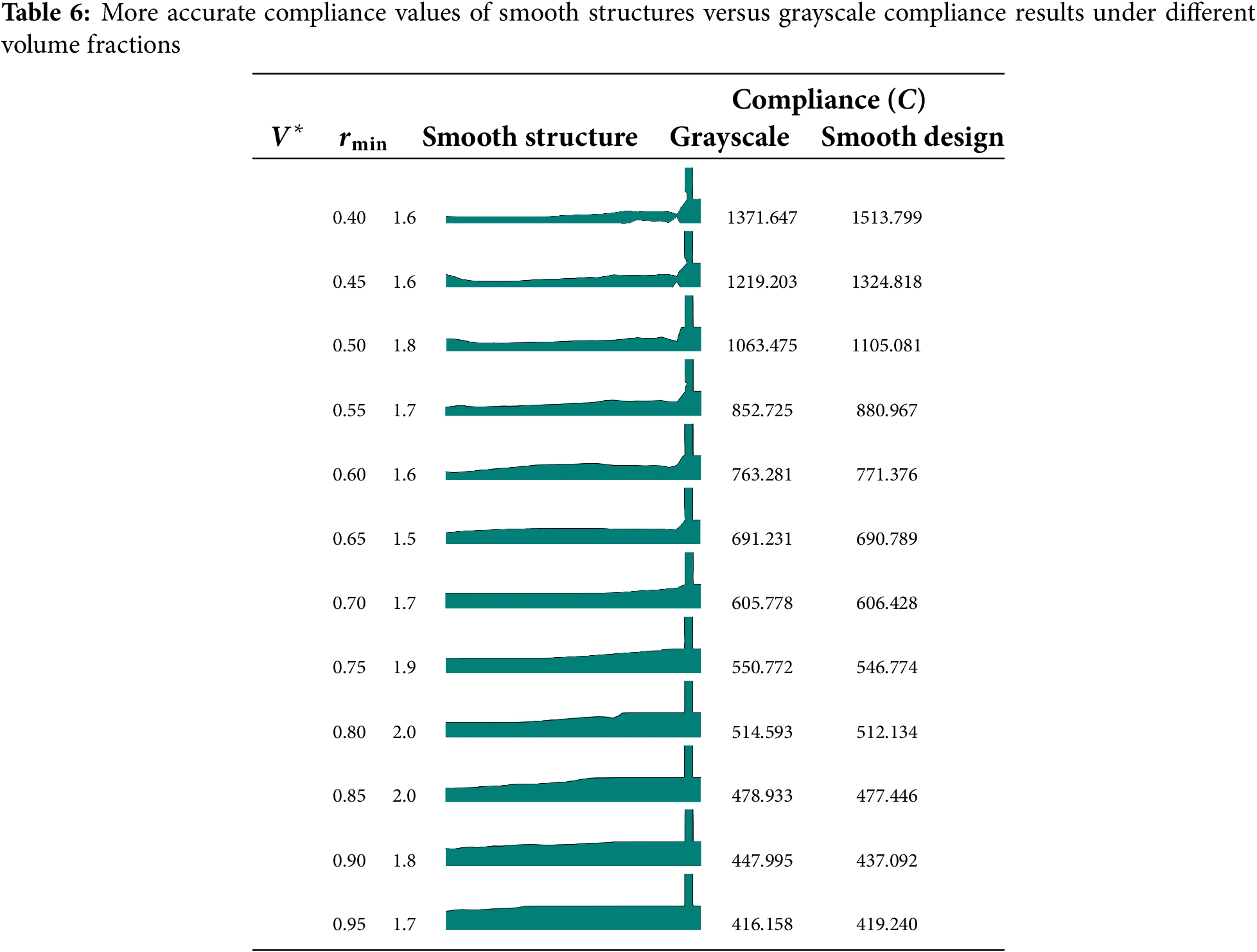
It should be noted that the compliance values of the smooth structures are comparable to those of grayscale structures for target volume fractions larger than 0.55. On the other hand, significant fluctuations appear at lower volume fractions, which can be attributed to two main factors: 1) increased geometric discrepancies between the grayscale and smooth structures due to the higher presence of grayscale elements, and 2) variations in the filter radius, which can negatively affect results, as illustrated in Fig. 8.

Hand-picking the best-performing smooth structures in SEMDOT, the resulting Pareto front is visualised in Fig. 13.

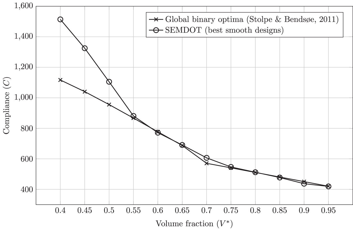
Figure 13: Pareto front of best-performing smooth SEMDOT results and the global binary optima [17]

Fig. 13 shows that when the best designs are selected, the more accurate compliance values for SEMDOT can closely approximate the global binary optima [17] for volume fractions higher than 0.55. At volume fractions of 0.6 and 0.9, SEMDOT results slightly surpass the global binary optima. This is due to the smooth boundary structures not being confined to the predefined mesh, allowing for more flexible shapes for boundary elements. At lower volume fractions, SEMDOT results deviate from global binary optima.

8  Conclusion

This study systematically benchmarks topology optimization methods using both the binary and relaxed forms of the ZR problem. Within this benchmarking framework, the SIMP method, SIMP with continuation, and the non-penalized SEMDOT method are compared. Through numerical tests, the main conclusions of this study are as follows:

1.   At comparable grayness levels, SEMDOT produces more optimal solutions for the ZR problem compared to the SIMP and continuation methods, mainly due to the usage of smooth Heaviside function, whereas SIMP and continuation methods rely on power-law approach. Furthermore, when the volume fraction is below 0.8, the topologies generated by SIMP (p=3) differ significantly from those of SEMDOT, continuation, and VTS methods. Tests indicate that none of the methods can achieve a continuous transition between the two global optima across the entire range of volume fractions. This is particularly challenging for all methods at volume fractions higher than 0.7, where the difference between the global binary and relaxed optima is minimal.

2.   All methods are influenced by the filter radius and mesh discretization, with SIMP and continuation methods being the most sensitive to changes in these parameters. SEMDOT is less sensitive, with its numerical results remaining almost consistent across different mesh resolutions and often achieving the lowest compliance. Notably, for finer meshes, SEMDOT generates structures that are closer to binary solutions (indicated by lower g values) compared to the other methods.

3.   Similar to other binary methods, the smooth designs produced by SEMDOT in the ZR problem can also become trapped in inefficient local optima due to tie breakage. Although adjusting the filter radius can partially mitigate this issue, it cannot be completely avoided across all volume fractions. A simple re-meshing approach used to assess the compliance of smooth designs more accurately shows that for volume fractions above 0.55, the best smooth design by SEMDOT performs comparably to the global binary optimum for the ZR problem.

Having a small number of finite elements, simple boundary conditions, and yet a challenging nature, the ZR problem serves as a convenient test case for different topology optimization methods. Apart from the above points, a key contribution of this study is the introduction of a simple-to-use benchmarking graph (Fig. 7) for the ZR problem. The proposed benchmarking graph can be used to quickly assess different topology optimization methods and benchmark them against global solutions and the well-established SIMP method.

However, this study primarily validates and benchmarks under the assumption of linear elasticity, while in practical structural design, material and geometric nonlinearities (such as plasticity and large deformations) often play a critical role. Future research could extend the linear elastic material model to more complex constitutive relations (e.g., von-Mises plasticity) and adopt Lagrangian formulations to introduce nonlinear stiffness matrices and large deformation effects in finite element solutions, thereby enhancing the overall applicability of benchmarked methods.

Acknowledgement: Jiye Zhou appreciates the financial support from the school: School of Engineering HDR.

Funding Statement: The authors received no specific funding for this study.

Author Contributions: The authors confirm contribution to the paper as follows: Conceptualization, Jiye Zhou, Yun-Fei Fu and Kazem Ghabraie; methodology, Jiye Zhou, Yun-Fei Fu and Kazem Ghabraie; software, Jiye Zhou; formal analysis, Jiye Zhou and Kazem Ghabraie; investigation, Jiye Zhou; writing—original draft preparation, Jiye Zhou; writing—review and editing, Jiye Zhou, Yun-Fei Fu and Kazem Ghabraie; visualization, Jiye Zhou and Kazem Ghabraie; supervision, Kazem Ghabraie. All authors reviewed the results and approved the final version of the manuscript.

Availability of Data and Materials: The data that support the findings of this study are available from the first author upon reasonable request.

Ethics Approval: Not applicable.

Conflicts of Interest: The authors declare no conflicts of interest to report regarding the present study.

References

1. Zhu J, Zhou H, Wang C, Zhou L, Yuan S, Zhang W. A review of topology optimization for additive manufacturing: status and challenges. Chin J Aeron. 2021;34(1):91–110. [Google Scholar]

2. Mallick PK. Materials, design and manufacturing for lightweight vehicles. Woodhead Publishing; 2020. [Google Scholar]

3. Wu J, Aage N, Westermann R, Sigmund O. Infill optimization for additive manufacturing-approaching bone-like porous structures. IEEE Trans Visual Comput Grap. 2017;24(2):1127–40. [Google Scholar]

4. Xie YM, Steven GP, Xie Y, Steven G. Basic evolutionary structural optimization. London, UK: Springer; 1997. [Google Scholar]

5. Yang XY, Xie YM, Steven GP, Querin OM. Bidirectional evolutionary method for stiffness optimization. AIAA J. 1999;37(11):1483–8. [Google Scholar]

6. Huang X, Xie Y. Convergent and mesh-independent solutions for the bi-directional evolutionary structural optimization method. Fin Elem Anal Des. 2007;43(14):1039–49. [Google Scholar]

7. Bendsøe MP. Optimal shape design as a material distribution problem. Struct Optim. 1989;1:193–202. [Google Scholar]

8. Sigmund O. On benchmarking and good scientific practise in topology optimization. Struct Multidiscipl Optim. 2022;65(11):315. [Google Scholar]

9. Bulman S, Sienz J, Hinton E. Comparisons between algorithms for structural topology optimization using a series of benchmark studies. Comput Struct. 2001;79(12):1203–18. [Google Scholar]

10. Rozvany G. Exact analytical solutions for some popular benchmark problems in topology optimization. Struct Optim. 1998;15:42–8. [Google Scholar]

11. Lewiński T, Rozvany G. Exact analytical solutions for some popular benchmark problems in topology optimization II: three-sided polygonal supports. Struct Multidis Optim. 2007;33(4):337–49. [Google Scholar]

12. Lewiński T, Rozvany G. Exact analytical solutions for some popular benchmark problems in topology optimization III: l-shaped domains. Struct Multidiscip Optim. 2008;35(2):165–74. [Google Scholar]

13. Stolpe M. On models and methods for global optimization of structural topology. Stockholm: Matematik; 2003. [Google Scholar]

14. Nguyen MN, Hoang VN, Lee D. Topology optimization framework for thermoelastic multiphase materials under vibration and stress constraints using extended solid isotropic material penalization. Compos Struct. 2024;344:118316. [Google Scholar]

15. Banh TT, Lieu QX, Kang J, Ju Y, Shin S, Lee D. A novel robust stress-based multimaterial topology optimization model for structural stability framework using refined adaptive continuation method. Eng Comput. 2024;40(2):677–713. [Google Scholar]

16. Nguyen MN, Hoang VN, Lee D. Multiscale topology optimization with stress, buckling and dynamic constraints using adaptive geometric components. Thin-Walled Struct. 2023;183:110405. [Google Scholar]

17. Stolpe M, Bendsøe MP. Global optima for the Zhou-Rozvany problem. Struct Multidis Optim. 2011;43:151–64. [Google Scholar]

18. Zhou M, Rozvany G. On the validity of ESO type methods in topology optimization. Struct Multidiscip Optim. 2001;21(1):80–3. [Google Scholar]

19. Edwards C, Kim H, Budd C. Investigation on the validity of topology optimisation methods. In: 47th AIAA/ASME/ASCE/AHS/ASC Structures, Structural Dynamics, and Materials Conference; 2006 May 1–4; Newport, RI, USA. [Google Scholar]

20. Edwards C, Kim H, Budd C. An evaluative study on ESO and SIMP for optimising a cantilever tie—beam. Struct Multidis Optim. 2007;34:403–14. [Google Scholar]

21. Rozvany GI, Querin OM. Combining ESO with rigorous optimality criteria. Int J Veh Des. 2002;28(4):294–9. [Google Scholar]

22. Rozvany GI. A critical review of established methods of structural topology optimization. Struct Multidis Optim. 2009;37:217–37. [Google Scholar]

23. Ghabraie K. The ESO method revisited. Struct Multidis Optim. 2015;51:1211–22. [Google Scholar]

24. Munk DJ, Vio GA, Steven GP. A bi-directional evolutionary structural optimisation algorithm with an added connectivity constraint. Fin Elem Anal Des. 2017;131:25–42. [Google Scholar]

25. Sigmund O, Aage N, Andreassen E. On the (non-)optimality of Michell structures. Struct Multidis Optim. 2016;54:361–73. [Google Scholar]

26. Sigmund O. Morphology-based black and white filters for topology optimization. Struct Multidis Optim. 2007;33:401–24. [Google Scholar]

27. Tarek M, Ray T. Adaptive continuation solid isotropic material with penalization for volume constrained compliance minimization. Comput Methods Appl Mech Eng. 2020;363:112880. [Google Scholar]

28. Fu YF, Long K, Rolfe B. On non-penalization SEMDOT using discrete variable sensitivities. J Optim Theory Appl. 2023;198(2):644–77. [Google Scholar]

29. Fu YF, Long K, Zolfagharian A, Bodaghi M, Rolfe B. Topological design of cellular structures for maximum shear modulus using homogenization SEMDOT. Mater Today Proc. 2024;101:38–42. [Google Scholar]

30. Kandemir V, Dogan O, Yaman U. Topology optimization of 2.5 D parts using the SIMP method with a variable thickness approach. Procedia Manuf. 2018;17:29–36. [Google Scholar]

31. Rozvany GI, Zhou M, Birker T. Generalized shape optimization without homogenization. Struct Optim. 1992;4:250–2. [Google Scholar]

32. Sigmund O, Petersson J. Numerical instabilities in topology optimization: a survey on procedures dealing with checkerboards, mesh-dependencies and local minima. Struct Optim. 1998;16:68–75. [Google Scholar]

33. Kawamoto A, Matsumori T, Yamasaki S, Nomura T, Kondoh T, Nishiwaki S. Heaviside projection based topology optimization by a PDE-filtered scalar function. Struct Multidis Optim. 2011;44:19–24. [Google Scholar]

34. Wang F, Lazarov BS, Sigmund O. On projection methods, convergence and robust formulations in topology optimization. Struct Multidiscip Optim. 2011;43(6):767–84. [Google Scholar]

35. Fu YF, Rolfe B, Chiu LN, Wang Y, Huang X, Ghabraie K. SEMDOT: smooth-edged material distribution for optimizing topology algorithm. Adv Eng Softw. 2020;150:102921. [Google Scholar]

36. Fu YF, Rolfe B, Chiu LNS, Wang Y, Huang X, Ghabraie K. Smooth topological design of 3D continuum structures using elemental volume fractions. Comput Struct. 2020;231:106213. [Google Scholar]

37. Fu YF, Ghabraie K, Rolfe B, Wang Y, Chiu LN. Smooth design of 3D self-supporting topologies using additive manufacturing filter and SEMDOT. Appl Sci. 2020;11(1):238. [Google Scholar]

38. Andreassen E, Clausen A, Schevenels M, Lazarov BS, Sigmund O. Efficient topology optimization in MATLAB using 88 lines of code. Struct Multidiscip Optim. 2011;43:1–16. [Google Scholar]

39. Bendsoe MP, Sigmund O. Topology optimization: theory, methods, and applications. Berlin/Heidelberg, Germany: Springer Science & Business Media; 2013. [Google Scholar]

40. Zhou J, Wang Y, NS L, Ghabraie K. On suitability of a simplified sensitivity estimation for partial elements in topology optimisation. Eng Optim. 2025;1–23. doi:10.1080/0305215X.2025.2466825. [Google Scholar] [CrossRef]

41. Szabó B, Babuška I. Finite element analysis: method, verification and validation. Hoboken, NJ, USA: John Wiley & Sons Inc.; 2021. [Google Scholar]

42. Hua Y, Luo L, Le Corre S, Fan Y. Heat spreading effect on the optimal geometries of cooling structures in a manifold heat sink. Energy. 2024;308:132948. [Google Scholar]

43. Huang X, Xie YM. A further review of ESO type methods for topology optimization. Struct Multidisc Optim. 2010;41(5):671–83. [Google Scholar]