Modeling and Simulation of Epidemics Using q-Diffusion-Based SEIR Framework with Stochastic Perturbations

1  Introduction

Epidemic modelling has historically been fundamental in comprehending and managing infectious diseases. The SEIR (Susceptible-Exposed-Infectious-Recovered) model is significant among many models due to its capacity to represent the dynamics of diseases with a latent period, like measles, influenza, and the new coronavirus. This model categorizes the population into four separate compartments, offering a framework to examine the transmission and potential control techniques for infectious illnesses.

The conventional SEIR model has been thoroughly examined; however, real-world situations frequently require adaptations to address more intricate dynamics, including spatial dispersion and atypical incidence rates. Incorporating diffusion factors in epidemic models facilitates the simulation of spatial dissemination, an essential element in comprehending small outbreaks and their potential progression into extensive epidemics. Conventional diffusion models presume uniform distribution; however, the emergence of q-diffusion provides a more generalized and adaptable methodology. Using non-linear diffusion processes as its foundation, q-diffusion is a parameterized diffusion model that accurately shows different spreading rates and changes in population density and movement patterns.

Advantages of the SEIR Framework:

1.    The SEIR model has an exposed (E) compartment that specifically reflects those infected but not yet contagious. Diseases with a notable incubation time and a lag between exposure and infectiousness are especially well-suited for the SEIR model.

2.    The SIR model (Susceptible-Infected-Recovered) presumes no latent period; people immediately become infectious following exposure. Though less accurate for diseases like COVID-19, measles, tuberculosis, or influenza when a delay between infection and infectiousness exists, it is appropriate for diseases with very short or insignificant incubation periods.

3.    COVID-19, measles, tuberculosis, and influenza show important transmission dynamics during incubation. Simpler models (like SIR) can produce false forecasts about outbreak time and control actions without explicitly incorporating this delay.

4.    Including the exposed class lets one more realistically model intervention tactics like contact tracing and quarantine that aim at people in the latent (exposed) stage before they become contagious.

5.    Additionally, the SEIR model framework improves the ability to estimate the basic reproduction number R∘ and the impact of early interventions is vital for planning effective public health responses.

Thus, the SEIR model forms a natural foundation for studying the spatial-temporal spread of infectious diseases, especially when combined with modern extensions like stochastic perturbations and generalized diffusion effects, as considered in this study.

Stochastic effects: Because actual disease transmission is naturally unpredictable owing to differences in human behavior, environmental variables, and intervention programs, stochastic effects are quite important. Deterministic models can miss the variety and uncertainty in case counts, especially in the early phases of outbreaks or small populations. Including stochasticity helps to more accurately portray epidemic dynamics, including the likelihood of disease extinction, outbreak variability, and random deviations around mean paths.

Spatial diffusion: Spatial diffusion explains why infectious diseases do not spread consistently. Transmission, on the other hand, is affected by local clustering, mobility patterns, and regional variation in contact rates. Spatially explicit models, particularly those including generalized diffusion such as q-diffusion, can mimic events like the wave-like spread of diseases or the generation of localized hotspots.

Studying infectious diseases and their transmission among populations is crucial in epidemiology for reducing outbreaks and developing efficient control techniques. Contagious diseases have consistently posed a significant issue for public health experts, academics, and policymakers globally. Understanding the evolution of epidemics is essential for formulating effective control methods and comprehending the complex interplay between human behaviour, environmental factors, and disease transmission.

The groundbreaking SIR (Susceptible-Infectious-Recovered) model, first presented in 1927 by pioneers Kermack and McKendrick [1], is the ancestor of the SEIR model. In their innovative study, they set out to investigate the mechanisms that control the spread of infectious diseases. An expansion of the SIR model, the SEIR model takes into account a crucial component of infectious diseases: the latent or incubation period. This better represents the real progression of numerous infectious diseases, including Ebola, HIV/AIDS, and COVID-19, wherein a person may be infected but not yet contagious. You can estimate an extra parameter using the supplied data when you include the “Exposed” compartment. As a result, key epidemiological factors such as the disease’s transmission rate and incubation period can be more precisely estimated. In recent years, extensive research has been conducted on the SEIR epidemic model, as evidenced by sources [2–5].

A vital component of contemporary epidemic modelling is the depiction of the incidence rate. Classical models frequently utilize a bilinear or mass-action incidence function, which may inadequately represent the intricacies of disease transmission dynamics. Integrating a generalized incidence rate considering behavioural modifications, and saturation effects improves the model’s precision and relevance [6].

The increasing complexity of these advanced models needs strong numerical methods that can accurately and stably capture their intricate dynamics. Analytical solutions for these models are frequently inaccessible because of the non-linear and stochastic characteristics of the governing equations, requiring the creation of effective computational methods [7]. A computational framework designed for the SEIR model incorporating q-diffusion and a generalized incidence rate can yield significant insights into disease dynamics, serving as a robust tool for decision-making for policymakers and healthcare professionals [8].

Not all populations experience the same rate of epidemic spread. An important factor in the spread of diseases is geographical heterogeneity, including human movement, age, population density, place, and physical obstacles. Epidemic models rely on diffusion, which considers the geographical spread of infectious diseases [9]. Policymakers can make educated judgments regarding resource allocation and intervention tactics using diffusion models, which incorporate geographical features, human mobility patterns, and contact networks. Since diseases might spread from one place to another, these models help determine which areas should receive vaccinations first, increasing the effectiveness of these programs in disease management.

Diffusion models can be broadly classified into two categories: local and non-local. In local diffusion, as described by the Laplacian operator, the primary factor influencing the spread of a phenomenon (in this case, a disease) is the degree to which it interacts with and is connected to nearby or neighbouring areas. Capone et al. [10] examine a reaction-diffusion SEIR model for infectious diseases, examining the non-linear asymptotic stability of the endemic equilibrium, studying long-term solution behaviour, and locating absorbing sets in phase space. In their analysis of a diffusive SEIR model with non-linear incidence, Han and Lei [11] highlighted the importance of the parameter in the persistence and extinction of diseases by concentrating on the global stability of the equilibria.

In contrast, the idea of non-local diffusion suggests that a phenomenon might extend over greater distances than just its immediate surroundings. Due to its mathematical attractiveness and large epidemiological insights, the non-local diffusion epidemic model has recently become a focal point of academics. Coville and Dupaigne [12] investigate a one-dimensional non-local variant of Fisher’s equation to understand better how genetic mutations spread across populations. The non-local diffusion pattern, which is thought to control the distribution of hereditary characteristics, is shown using a convolution operator.

The non-local diffusion equation and the classical heat equation with the Neumann boundary condition share many commonalities, as shown in studies by Cortazar et al. [13,14]. These include the following: the solutions to both equations exhibit similar asymptotic behaviour as t→∞, and both equations adhere to the maximum principle.

Much recent research has investigated SIR, SIS, and SVIR, among others, as epidemic models in the context of non-local spread. A basic SIR model with non-local diffusion was the subject of recent work by Kuniya and Wang [15], who sought to prove that its equilibrium was stable on a global scale. In their investigation of an epidemic model involving free boundaries and non-local diffusion, Zhao et al. [16] detail the spread of infectious organisms through such a model and the lack of diffusion in the case of sick humans. In contrast to local diffusion models, their results show distinct solutions and a binary between spreading and vanishing; picking a non-local diffusion kernel function might speed up the spreading process. Disease management, primarily through increased vaccination rates, is emphasized in [17], presenting a qualitative analysis of an SVIR epidemic model incorporating non-local dissemination. New insights into non-local diffusion epidemic models, including several infected compartments, were provided by Zhang and Zhao [18], who investigated travelling wave solutions in a non-local diffusive Zika transmission model using bilinear incidence. In their discussion of treat-age effects in a non-local dispersal SIR epidemic model, Bentout and Djilali [19] examine the asymptotic profiles. According to their research, the disease can only be contained if more people are treated more quickly. Djilali et al. [20] thoroughly examine a SIR epidemic model in a heterogeneous environment with non-local diffusion and non-linear incidence, focusing on studying the global stability of equilibrium states.

Measles, tuberculosis, and influenza are just a few infectious diseases that have prompted the development and analysis of several epidemic models in recent years [21,22]. Bilinear incidence rate βSI is commonly employed in numerous epidemic models [23]. Esteva and Matias [24] proposed the saturated incidence rate βSI1+αI, which approaches a saturation threshold as I increases. Here, βI quantifies the infection force when the disease infiltrates a completely susceptible population while 11+αI reflects the inhibitory effect of susceptible individuals’ behavioural modifications as their population grows or from the crowding effect of infective individuals. This incidence rate is more rational than the bilinear incidence rate since it incorporates behavioural changes and the crowding effect of infectious persons, averting the contact rate’s unboundedness by selecting appropriate parameters. Subsequently, it was utilized in numerous epidemic models (see to, for instance, [24,25]).

Treatment is a crucial and successful strategy for preventing and controlling the dissemination of infectious diseases. Classical epidemic models posit that the treatment rate of infection is proportional to the number of infected individuals; however, the recovery rate is generally contingent upon medical resources, including pharmaceuticals, vaccinations, hospital capacity, isolation facilities, and treatment efficacy. Recognizing that each community or nation possesses finite resources for illness management, it is imperative to implement an appropriate treatment strategy. Wang and Ruan [26] presented a continual intervention within a SIR model as follows:

h(I)={r,I>00,I=0,

which replicated a constrained capacity for therapy. Additionally, Wang [27] examined the subsequent piecewise linear treatment function:

h(I)={rI,0≤I≤I∘rI∘,I>I∘,

where I∘ is the infective level at which the healthcare system attains capacity; specifically, treatment escalates linearly with I until capacity is reached, after which it assumes its maximum value of rI∘. This appears more rational than the typical linear function. In [28], J. C. Eckalbar and W. L. Eckalbar developed a SIR model with a quadratic treatment function as detailed below:

T(I)=max{rI−gI2,0},r,g>0.

Furthermore, the efficacy of treatment will be significantly compromised if infected persons experience delays in receiving care. In [29], Zhang and Liu employed a continuous and differentiable saturation therapy function h(I)=rI1+kI, where r>0 represents the cure rate, and the parameter k quantifies the degree of delay in treatment for the infected individuals. The treatment function h(I) converges to rI for small values of I, whereas for large values of I, h(I) approaches rk. It is more realistic and offers the advantages of continuity and differentiation compared to its predecessors.

Despite the widespread use of SIR or SIS epidemic models with a saturated incidence rate in numerous literatures [30–32], the saturated treatment function in SEIR epidemic models has received surprisingly little attention.

Many scientists are now focusing on finding solutions to non-linear differential equations that describe many events. Current society is primarily focused on c-calculus and partial differential equations. Euler and Jacobi formulated the history of c-calculus in the seventeenth century. Jackson [33] was a trailblazer in the 20th century who built on the work of Euler and Jacobi. Several mathematical and analytical subfields discovered broad uses for c-calculus in the mid-twentieth century, leading to a dramatic upsurge in its study. In recent times, c-calculus has been relevant to mathematical modelling in quantum computing. Read [34,35] for more information.

Recent developments in epidemic modelling have revealed an increasing intersection between classical compartmental models (e.g., SIR, SEIR) and data-driven methods like machine learning (ML) and deep learning (DL). While conventional models give interpretability and control over biological assumptions, ML/DL methods offer great prediction power, particularly when real-time data are plentiful. Many papers have suggested hybrid models combining the mathematical framework of SEIR models with the learning ability of neural networks to forecast future case trends or estimate parameters more precisely. The work of Chumachenko et al. [36], for example, reveals the use of deep learning for real-time epidemic forecasting, indicating that such models can better capture non-linear dynamics and data anomalies than purely theoretical approaches. Recent studies have likewise used convolutional and recurrent neural networks to model spatial-range diffusion processes. Our present work emphasizes a high-order deterministic and stochastic numerical framework. However, it supports data-driven approaches by offering a theoretically strong basis that might be improved with ML for real-time relevance.

A new subfield of mathematics, the q-calculus, investigates the connection between the two fields. The field of q-calculus is regarded as a main resource for research in various branches of mathematics, including number theory, combinatorics, basic hypergeometric functions, quantum theory, and orthogonal polynomials. This area has developed a novel approach to differential transform methods appropriate for numerically solving ordinary and partial differential equations.

The q-differential equation originated in this subject, which accounts for several physical processes in quantum dynamics, discrete dynamical systems, and discrete stochastic processes. Please note that q-differential equations are defined on a time scale denoted as Tq, where q is the scale index. Based on q-calculus theory, several other concepts have been introduced and familiarized, such as q-Laplace transforms, q-Gamma and q-Beta functions, q-Mittag–Leffler functions, q-Taylor expansion, and q-integral transform theory. References [37–41] provide further information on q-calculus and q-partial differential equations. Comparatively, fractional q-calculus is a less advanced field of study.

Particularly in epidemiological systems with variable spatial interactions, the adoption of q-diffusion in this work is driven by its capacity to generalize classical diffusion while maintaining local behavior. Unlike classical diffusion, which assumes consistent spatial spreading, and fractional diffusion, which simulates long-range memory effects, q-diffusion offers a non-linear generalization that captures unusual yet localizable transport dynamics. Modeling scenarios where non-uniform interaction structures, spatial clustering, or intervention actions change movement patterns in non-classical ways that influence disease transmission is especially beneficial.

This work presents a new computational method for addressing the SEIR epidemic model enhanced by q-diffusion and a generalized incidence rate. The scheme employs a high-order spatial discretization method to handle the q-diffusion term and a time-stepping algorithm for stability and accuracy. The suggested scheme’s stability and convergence are thoroughly examined, and its performance is compared to existing approaches.

The main contributions of this study are as follows:

1.    Formulation of an SEIR epidemic model incorporating q-diffusion and a generalized incidence rate.

2.    Development of a computational scheme that achieves high accuracy in both temporal and spatial domains.

3.    Stability and convergence analysis to ensure reliability in simulations.

4.    Application of the proposed model to a case study, demonstrating its capability to simulate realistic epidemic scenarios.

This study intends to close the gap between recent theoretical developments in epidemic modelling and their actual use in practice using computational methods. This research adds to the growing body of practical and adaptable epidemic analysis methods by enhancing the SEIR framework with q-diffusion and generalized incidence rates.

The remainder of the article is structured as follows: Section 2 presents the suggested numerical scheme and the stability and consistency studies in Section 3. With q-diffusion, Section 4 shows the development of the stochastic SEIR model. Section 5 offers a comparative study with current techniques and numerical experiments. Finally, Section 6 wraps up the paper and suggests possible avenues for future investigation.

2  Proposed Computational Scheme

This scheme is a predictor-corrector method for SPDEs with q-diffusion effects applied to an SEIR epidemic model. Using high-order accuracy and stability, the goal is to numerically simulate how an infectious disease spreads spatially and stochastically in a population. A numerical scheme will be presented that will solve stochastic time-dependent partial differential equations. A numerical scheme for the deterministic model is proposed before proposing a numerical scheme for stochastic partial differential equations. The proposed numerical scheme is a predictor-corrector scheme that requires a solution calculated on nth time level and its corrector stage to find the solution at (n+1)th time level. Although the predictor scheme finds the solution at an arbitrary time level. To construct a numerical scheme for the deterministic model, consider a differential equation as

∂f∂t=β∂2f∂x2+F(f).(1)

This is a reaction-diffusion equation, where f(x,t) represents a population density (e.g., infected individuals), β∂2f∂x2: describes diffusion spatial spread of the disease, β is constant, and F(f) models the reaction (e.g., infection or recovery dynamics).

2.1 Predictor Stage (Exponential Integrator)

The first stage of the proposed scheme is constructed as

f¯in+1=0.5fine2Δt+0.5fine−Δt+(e2Δt+e−Δt−2){∂f∂t|in−0.5fin},(2)

where Δt represents temporal step size, this predicts the solution at an intermediate time step f¯in+1 using an exponential form. Exponential integrators help with stiff equations, which are common in epidemic models where sudden spikes (outbreaks) can occur. The predictor estimates how the number of people in a compartment (say, exposed or infected) changes quickly. This estimate is crucial for scenarios like lockdown planning or vaccination rollout timing.

The first stage of the scheme (2) can be considered a modified exponential integrator that can be used separately to find the first-order accurate solution of time-dependent partial differential equations. However, a predictor stage finds the solution at some arbitrary time level in this condition.

2.2 Corrector Stage

The second stage of the proposed scheme is presented as

fin+1=afin+bf¯in+1+c(eΔt−1){∂f¯∂t|in+1},(3)

where a,b, and c are unknown parameters that will be found by matching Taylor series expansion to ensure second-order accuracy. Combines past state fin, predicted value fin+1, and rate of change to correct the prediction. This will ensure that disease dynamics follow realistic trends, capturing smooth and abrupt changes.

2.3 Solve for Coefficients via Taylor Expansion

To find these parameters, substitute the first stage of the proposed scheme (2) with the second stage (3).

fin+1=afin+b(0.5fine2Δt+0.5fine−Δt+(e2Δt+e−Δt−2){∂f∂t|in−0.5fin})+c(eΔt−1)(0.5e2Δt∂f∂t|in+0.5e−Δt∂f∂t|in+(e2Δt+e−Δt−2){∂2f∂t2|in−0.5∂f∂t|in}),(4)

By using the Taylor series expansion fin+1 can be expanded as

fin+1=fin+Δt∂f∂t|in+(Δt)22∂2f∂t2|in+O((Δt)3).(5)

By substituting Eq. (5) into Eq. (4) it is obtained

fin+Δt∂f∂t|in+(Δt)22∂2f∂t2|in=afin+b(0.5fine2Δt+0.5fine−Δt+(e2Δt+e−Δt−2){∂f∂t|in−0.5fin})+c(eΔt−1)(0.5e2Δt∂f∂t|in+0.5e−Δt∂f∂t|in+(e2Δt+e−Δt−2){∂2f∂t2|in−0.5∂f∂t|in}).(6)

Now, equating the coefficients of fin,∂f∂t|inand ∂2f∂t2|in on both of Eq. (6), it is obtained

1=a+bΔt=b(e2Δt+e−Δt−2)+c(eΔt−1)(0.5e2Δt+0.5e−Δt−0.5(e2Δt+e−Δt−2))(Δt)22=c(eΔt−1)(e2Δt+e−Δt−2)}.(7)

This will ensure the scheme’s time accuracy and stability by matching terms order by order. There are no arbitrary coefficients, and everything is mathematically consistent.

By solving linear Eq. (7), the values in the form of expression can be obtained.

So, the time discretization scheme for the deterministic model (1) can be expressed as

f¯in+1=0.5fine2Δt++0.5fine−Δt+(e2Δt+e−Δt−2){β∂2f∂x2|in+F(fin)−0.5fin},(8)

fin+1=afin+bf¯in+1+c(eΔt−1){β∂2f¯∂x2|in+1+F(f¯in+1)}.(9)

2.4 Space Discretization Using Compact Scheme

Space discretization is performed by employing a compact scheme. The compact scheme for this can be written as

f¯in+1=0.5fine2Δt++0.5fine−Δt+(e2Δt+e−Δt−2){P−1Qfin+F(fin)−0.5fin},(10)

fin+1=afin+bf¯in+1+c(eΔt−1){P−1Qf¯in+1+F(f¯in+1)}.(11)

where P and Q are matrices that are constructed by the coefficients of the left-hand and right-hand sides of the following equations

β1f″|i−1n+f″|in+β1f″|i+1n=c∘(fi+1n−2fin+fi−1n)(Δx)2+c1(fi+2n−2fin+fi−2n)4(Δx)2,(12)

where c∘=4/3(1−β1),c1=1/3(10β1−1) and β1 refers to a weighting parameter used for approximating the second-order spatial derivative.

This compact scheme will give sixth-order accuracy in space and capture fine-scale spatial disease variations (e.g., infections clustered in a city).

2.5 Incorporate Stochasticity

Now consider the stochastic differential equation as

∂f=β∂2f∂x2dt+F(f)dt+σfdW,(13)

where W stands for the Wiener process and σfdW: stochastic noise scaled by the current state. In this equation, we added randomness to model unpredictable fluctuations like sudden super-spreader events or variability in transmission rates.

2.6 Stochastic Scheme

The first stage of the proposed scheme for Eq. (13) is the same for the deterministic model, i.e., Eq. (10). While the second stage of the proposed scheme considered is expressed as

fin+1=afin+bf¯in+1+c(eΔt−1){P−1Qf¯in+1+F(f¯in+1)}+σfinΔW,(14)

where ΔW∼(Wn+1−Wn) is approximated as a normal distribution N(0,Δt). We added the stochastic term σfΔW to the deterministic corrector. These equations model day-to-day disease transmission unpredictability due to human behaviour, weather, interventions, etc. All numerical simulations presented in this paper are based on this discrete scheme, which combines a high-order compact spatial discretization with a modified exponential integrator for time evolution.

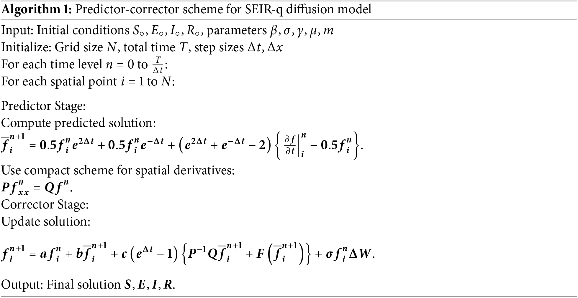
We developed a predictor-corrector type computational method in our work that efficiently resolves stochastic partial differential equations essential to epidemic modelling. Using a modified exponential integrator, which is well-suited for capturing fast changes in disease dynamics, the system starts with a predictor stage, offering an initial approximation of the solution. In the corrector stage, this predicted value is adjusted using a mix of current and projected values and their rates of change. The time discretization parameters are carefully selected using Taylor series expansion to guarantee accuracy and stability. A sixth-order compact technique is used for spatial discretization, enabling us to precisely capture fine-scale changes in disease transmission. A stochastic factor is included to reflect natural unpredictability in the transmission of illnesses, such as changes in contact rates or external influences like policy changes, making the model more realistic. This approach provides a consistent, precise, and effective instrument for simulating how an infectious illness spreads over time and location in a population, which is pertinent for public health forecasting and control policies.

3  Stability Analysis

Fourier series analysis or Von Neumann stability analysis is one of the existing criteria for checking the stability conditions of existing finite difference schemes. The criterion provides conditions for temporal and spatial step sizes of the schemes. The analysis gives the exact stability conditions of the numerical scheme of linear partial differential equations and estimates the numerical scheme of non-linear partial differential equations. However, the non-linear partial differential equation must be linearized before applying this analysis. To apply this analysis in this contribution, transformations must be considered

PeiIζ=β1e(i+1)Iζ+eiIζ+β1e(i−1)Iζ,(15)

QeiIζ=c∘(e(i+1)Iζ−2eiIζ+e(i−1)Iζ)(Δx)2+c1(e(i+2)Iζ−2eiIζ+e(i−2)Iζ)4(Δx)2,(16)

where β1 refers to a weighting parameter used in constructing the sixth-order compact finite difference scheme for approximating the second-order spatial derivative, and ζ represents a generic auxiliary variable or parameter.

By applying transformations (15), (16) for the first stage of the scheme (10) gives with F=0, and it is obtained

f¯in+1=0.5fine2Δt+0.5fine−Δt+(e2Δt+e−Δt−2){β(4c∘(cosζ−1)+c1(cos2ζ−1)2(Δx)2(2β1cosζ+1))−0.5}fin,(17)

where f¯in+1 denotes the intermediate predicted solution at spatial grid point i and time level n+1, obtained from the predictor stage of the proposed scheme. Eq. (17) can be written as

f¯in+1=αfin,(18)

where α=0.5e2Δt+0.5fine−Δt+(e2Δt+e−Δt−2){β(4c∘(cosζ−1)+c1(cos2ζ−1)2(Δx)2(2β1cosζ+1))−0.5}.

By applying the transformations (15), (16) into the second stage of the proposed scheme (14) using F=0 it, yields

fin+1=afin+bf¯in+1+c(eΔt−1){β(4c∘(cosζ−1)+c1(cos2ζ−1)2(Δx)2(2β1cosζ+1))}f¯in+1+σfinΔW.(19)

Using Eq. (18) in Eq. (19) can be written as

fin+1=α1fin+σfinΔW,(20)

where α1=a+bα+c(eΔt−1){β(4c∘(cosζ−1)+c1(cos2ζ−1)2(Δx)2(2β1cosζ+1))}α.

The amplification factor for this case is written as

fin+1fin=α1+σΔW.(21)

The following equation can be obtained from Eq. (21).

E|fin+1fin|2≤2E|α1|2+2σ2E|ΔW|2.(22)

If |α1|2<1 and assume that 2σ2=λ the resulting Eq. (22) is written as

E|fin+1fin|2≤1+λΔt.(23)

Theorem 1: The proposed numerical scheme for time and compact spatial discretization is consistent in a mean square sense with F=0.

Proof 1: Let U be the smooth function, then

L(U)in=U((n+1)Δt,iΔx)−U(nΔt,iΔx)−β∫nΔt(n+1)ΔtUxx(s,iΔx)dS−σ∫nΔt(n+1)ΔtU(s,iΔx)dW(s),(24)

LinU=U((n+1)Δt,iΔx)−U(nΔt,iΔx)−b(e2Δt+e−Δt−2)P−1QU(nΔt,iΔx)−c(e2Δt−1)P−1QU¯((n+1)Δt,iΔx)−σU(nΔt,iΔx)(W((n+1)Δt)−W(nΔt)),(25)

where U¯((n+1)Δt,iΔx) = U(nΔt,iΔx)e2Δt + U(nΔt,iΔx)e−Δt+(e2Δt+e−Δt−2){P−1QU(nΔt,iΔx)−0.5U(nΔt,iΔx)}.

The expected value of the square of difference Eqs. (24) and (25) gives

E|L(U)in−LinU|2=E|−β∫nΔt(n+1)ΔtUxx(s,iΔx)dS−σ∫nΔt(n+1)ΔtU(s,iΔx)dW(s)+b(e2Δt+e−Δt−2)P−1QU(nΔt,iΔx)+c(e2Δt−1)P−1QU¯((n+1)Δt,iΔx)+σU(nΔt,iΔx)(W((n+1)Δt)−W(nΔt))|2,(26)

Eq. (26) can be expressed as

E|L(U)in−LinU|2≤2β2E|∫nΔt(n+1)ΔtUxx(s,iΔx)dS−b(e2Δt+e−Δt−2)P−1QU(nΔt,iΔx)−c(e2Δt−1)P−1QU¯((n+1)Δt,iΔx)|2+2σ2E|∫nΔt(n+1)ΔtU(s,iΔx)dW(s)−U(nΔt,iΔx)(W((n+1)Δt)−W(nΔt))|2.(27)

By using the inequality

E|∫t∘tv(s,w)dW(s)|2m≤(t−t∘)m−1[m(2m−1)]m∫t∘tE[|v(s,w)|2m]ds.(28)

By using inequality (28) into inequality (27) it yields

E|L(U)in−LinU|2≤2β2E|∫nΔt(n+1)ΔtUxx(s,iΔx)dS−b(e2Δt+e−Δt−2)P−1QU(nΔt,iΔx)−c(e2Δt−1)P−1QU¯((n+1)Δt,iΔx)|2+2σ2Δt∫nΔt(n+1)ΔtE|U(s,iΔx)dW(s)−U(nΔt,iΔx)(W((n+1)Δt)−W(nΔt))|.(29)

By applying the limit as Δx→0,Δt→0,t=(n+1)Δt and (nΔt,iΔx)→(t,x), then the mean square error tends to zero, i.e.,

E|L(U)in−LinU|2→0.(30)

Thus, it is proven that the proposed scheme in time and compact space is consistent in the mean square sense. □

4  Mathematical Model

A mathematical model of SEIR is expressed with a bilinear incident rate. The model is comprised of four compartments: susceptible, exposed, infected, and recovered. Let S(x,t) represents susceptible people (can catch the disease), E(x,t) represents exposed people (infected but not yet infectious), I(x,t) represents infectious people (can spread the disease) and R(x,t) represents recovered people (gained immunity or removed from the population). Let β represent the transmission rate at which susceptible people become exposed due to the interaction of infectious and susceptible people, μ represents the natural death and birth rate, the rate at which exposed people are infected is represented by σ, γ is the recovery rate, di,i=1,2,3,4 q-diffusion coefficients for each compartment, σi,i=1,2,3,4: noise intensity for each equation and W(t) Wiener process (models randomness in disease transmission). Let E∘,I∘are not zero at the same time. Let N represent the size of the population, which is supposed to be constant. The total population is N=S+E+I+R, which is assumed to be constant (birth and death rates balance each other). The number of recovered people is given as R=N−S−E−I. The disease will spread in the population if susceptible people become exposed and, after some time, are exposed to it. The stochastic mathematical model with q-diffusion effect is expressed as

∂S∂t=d1∂q2S∂x2−μS+μN−βIS1+mI2+σ1SW(t),(31)

∂E∂t=d2∂q2E∂x2+βIS1+mI2−μE−σE+σ2EW(t),(32)

∂I∂t=d3∂q2I∂x2+σE−μI−γI+σ3IW(t),(33)

∂R∂t=d4∂q2R∂x2+γI−μR+σ4RW(t).(34)

Susceptible Class Eq. (31): d1∂q2S∂x2: represents the movement/spread of susceptible people across space (q-diffusion), −μS+μN: represents natural death and birth; replenishing susceptible class, −βIS1+mI2: represents infection terms using saturated incidence models, how disease transmission slows down when the infected population becomes large (realistic in pandemics due to public awareness or interventions), and σ1SW(t) denotes the stochastic fluctuation (e.g., random behaviour in contacts or interventions).

Exposed Class Eq. (32): d2∂q2E∂x2: represents the movement or spatial spread of exposed individuals across the domain using q-diffusion. This helps model situations where exposed individuals (who are infected but not yet infectious) may move from one region to another, βIS1+mI2: represents the gain in the exposed class due to contact between susceptible and infectious individuals, using a saturated incidence rate. This reflects the realistic slowdown in transmission when the number of infectious individuals becomes large (due to behavioural changes, interventions, etc.), −μE: represents the natural death of exposed individuals, −σE: represents the progression of exposed individuals to the infectious class at rate σand σ2EW(t): denotes stochastic fluctuation in the exposed population—could be due to variability in incubation periods or delays in detection and reporting.

Infectious Class Eq. (33): d3∂q2I∂x2: represents the spatial spread of infectious individuals via q-diffusion. This accounts for individuals moving between regions, potentially spreading diseases, σE: represents the transition of individuals from the exposed class to the infectious class as they become symptomatic or capable of transmitting the disease, −μI: represents the natural death of infectious individuals, −γI: represents the recovery of infectious individuals at rate γ, leading them to move into the recovered class and σ3IW(t): represents stochastic variability in the infection dynamics, such as unexpected outbreaks, random changes in contact behaviour, or testing fluctuations.

Recovered Class Eq. (34): d4∂q2R∂x2: describes the spatial redistribution of recovered individuals, e.g., movement of immune people across different regions, γI: represents the inflow into the recovered class as infectious individuals recover from the disease, −μR: accounts for the natural death of recovered individuals and σ4RW(t) denotes random fluctuations in the recovered class, possibly due to loss of immunity, reinfections, or inconsistencies in immunity duration.

Subject to the initial conditions

S∘=g1(x),E∘=g2(x),I∘=g3(x),R∘=g4(x).(35)

These are the initial distributions of each class over space. It reflects the geographical spread of the disease at the beginning (e.g., urban vs. rural infections).

And boundary conditions are expressed as

∂S∂x=0,∂E∂x=0,∂I∂x=0,∂R∂x=0,(36)

represents the No-flux boundary conditions, no movement in/out at domain boundaries, this means the region is closed (like an isolated city or quarantined area)

Choice of Functional Form: The interaction function used in this study is a saturated incidence rate given by Interaction term=βIS1+mI2. This form was chosen to reflect the non-linear transmission dynamics observed in real epidemics, particularly when the number of infected individuals becomes large. Traditional bilinear incidence βSI assumes that the infection rate grows indefinitely with I, which is not realistic during large outbreaks. In contrast, the saturation term 1+mI2 limits the growth of infection transmission, making the model more biologically meaningful under high infection pressure. The saturated form reflects several biological and behavioral mechanisms: As the number of infected individuals increases, people reduce their contacts voluntarily (social distancing, increased caution) or through imposed public health measures (lockdowns, travel restrictions). High infection levels can overload healthcare systems, indirectly reducing the number of new infections due to constrained movement and reduced effective contacts. We believe that using this interaction function greatly improves the realism of the SEIR model in pandemic contexts such as COVID-19.

Disease-Free Equilibrium (DFE) Eqs. (37)–(41):

The disease-free equilibrium (steady state without disease) for ordinary differential equations can be found by setting

−μS+μN−βIS1+mI2=0,(37)

βIS1+mI−μE−σE=0,(38)

σE−μI−γI=0,(39)

γI−μR=0.(40)

By solving Eqs. (37)–(40) the disease-free equilibrium points can be found as

B∗=(S,E,I,R)=B∗(N,0,0,0).(41)

This means everyone is susceptible, with no current infections or recoveries.

Derivation of R∘: For the proposed SEIR model with q-diffusion (ignoring spatial effects for local stability analysis), the disease transmission dynamics can be approximated by the system of ordinary differential equations:

dSdt=µ(N−S)−βIS1+mI2,(42)

dEdt=βIS1+mI2−(µ+σ)E,(43)

dIdt=σE−(μ+γ)I,(44)

dRdt=γI−μR.(45)

Using the Next Generation Matrix (NGM) approach, R∘ can be derived as

R∘=βNσ(μ+σ)(μ+γ).(46)

Dependence of R∘ on Key Parameters: Transmission rate β: Directly proportional to R∘; higher β increases the potential for an outbreak. Progression rate σ: Also positively related to R∘; the faster progression from exposure to infection increases the effective number of secondary cases. Recovery rate γ: inversely proportional to R∘; faster recovery reduces the time individuals remain infectious. Natural death rate μ: acts to decrease R∘ slightly, but in most epidemic models, μ is relatively small compared to epidemic time scales. It is important to note that while q-diffusion alters the spatial dynamics, it does not directly affect the local value of R∘, which is determined by temporal (non-spatial) dynamics.

Implications of R∘ for Disease Control Strategies: If R∘>1, the infection can invade and persist in the population; control strategies must be implemented to bring R∘ below 1. Reducing β through social distancing, vaccination, or mask-wearing is critical. Increasing γ by improving treatment rates, or σ by early diagnosis and isolation, can also indirectly help control the epidemic. Although spatial diffusion influences how fast and where the disease spreads, controlling R∘ remains central to overall epidemic suppression.

Theorem 2: The system of ordinary differential equations by putting d1=0=d2=d3=d4 and σ1=0=σ2=σ3=σ4 in Eqs. (31)–(34) is locally stable if γ2−2γσ+4βNσ<4(μ+σ2+γ2)2 or γ2+σ2+4Nβσ<2γσ.

Proof 2: The Jacobian system of ordinary differential equations corresponding to Eqs. (33)–(36) is expressed as

J=[−μ−βI1+mI0−βS1+mI2+βImS(1+mI)20βI1+mI2−μ−σβS1+mI2−2βmSI2(1+mI2)200σ−γ−μ000γ−μ].(47)

The Jacobian at disease-free equilibrium points B∗ is expressed as

J|B=[−μ0−βN00−μ−σβN00σ−γ−μ000γ−μ].(48)

The eigenvalues of the matrix (48) are expressed as

λ1=−μ,λ2=−γ2−μ−σ2−γ2−2γσ+σ2+4βNσ2,λ3=−μ−σ2−γ2+γ2−2γσ+σ2+4βNσ2.

For the real part of all eigenvalues to be negative, the expression under the square root must not overcome the negative term in λ3. That leads to the following condition: γ2−2γσ+4βNσ<4(μ+σ2+γ2)2 or equivalently γ2+σ2+4Nβσ<2γσ. These conditions ensure that λ3<0, meaning no solution components grow exponentially, i.e., infection will die out.

The future work will address the stability and bifurcation analysis of the endemic equilibrium, potentially using numerical continuation and Lyapunov-based approaches. □

5  Results and Discussions

The suggested technique is designed to address both deterministic and stochastic scenarios. The approach can be seen as an enlarged version of the Euler-Maruyama method. The Euler-Maruyama method incorporates a singular component for stochastic models, while the remainder is the Euler method. The Euler approach offers first-order temporal precision. The suggested system extends the first-order Euler method for deterministic models. It addresses the Wiener process term in stochastic differential equations in a manner analogous to the Euler method. The Euler technique is formulated as a single-stage process, whereas the proposed scheme is developed as a two-stage process. The Von Neumann stability analysis indicates that the method is conditionally stable, imposing limits on step sizes and associated parameters. A stable solution can be achieved if the scheme meets the stability criteria. Thus, the fulfillment of stability is essential for obtaining a convergent solution.

For simulation, we take the birth/death rate μ=0.1, transmission rate β=0.1, progression rate σ=0.1, recovery rate γ=0.3, total population size N is 1. Furthermore, σi=0.1, di=0.1 for i=1,2,3,4.

To determine the eigenvalues of the Jacobian matrix at the disease-free equilibrium (DFE) B∗ for the given parameter values, note that at the equilibrium state, S=N=1, and E=I=R=0, which gives,

J|B∗=[−0.10−0.100−0.20.1000.1−0.40000.3−0.1]

Then, solving the characteristic equation |J−λI|=0, i.e.,

|−0.1−λ0−0.100−0.2−λ0.1000.1−0.4−λ0000.3−0.1−λ|=0,

we obtain the eigenvalues,

λ1=−0.1,λ2=−0.1,λ3=−0.4414 and λ4=−0.1586.

Since all eigenvalues are real and negative, the disease-free equilibrium B∗is locally asymptotically stable. This supports the theoretical result in Theorem 2 for the chosen parameter values, meaning the infection will not spread if introduced in small amounts.

Numerical Implementations details: All numerical simulations presented in this paper are based on a discrete scheme combining a high-order compact spatial discretization with a modified exponential integrator for time evolution. All simulations are conducted using uniform grids in space and time. Zero-flux (Neumann) boundary conditions are applied. The initial conditions are discretized based on predefined spatial profiles. Stochastic terms are implemented via independently generated Gaussian noise at each time step and spatial location. The method is implemented in MATLAB, and step sizes are chosen to ensure numerical stability. This numerical framework has been consistently applied to all simulations and figures this study presents. The simulations were performed on a standard personal computer with an Intel Core i7 processor (2.6 GHz) and 16 GB RAM. No parallel processing or GPU acceleration was used. The proposed scheme involves two stages per time step and utilizes a sixth-order compact spatial discretization. The time complexity per time step is O(N), where N is the number of spatial nodes. Matrix inversion in the compact scheme uses a tridiagonal structure, allowing efficient implementation.

5.1 Effect of Transmission Rate β on Susceptible Population (Fig. 1)

Fig. 1 shows the variation in the susceptible population over time for different values of the transmission rate β, while keeping other parameters fixed: μ=0.1,γ=0.3,q=0.5,σ=0.1,m=0.01,d1=0.1,d2=0.1,d3=0.1,d4=0.1,σ1=0.1,σ2=0.1,σ3=0.1,σ4=0.1. As the value of β increases from 0.3 to 0.5, the decline in the susceptible population becomes more pronounced. This behaviour is consistent with the role of β as the transmission rate, which governs how quickly susceptible individuals become exposed due to interactions with infected individuals. A higher β leads to more frequent transitions from the susceptible to the exposed class, resulting in a faster depletion of the susceptible group. The figure also includes stochastic effects (due to non-zero σ1) and q-diffusion (non-zero d1), which introduces variability and spatial influence into the dynamics. Despite this, the overall trend shows that increased transmission intensity leads to a steeper and earlier drop in the number of susceptible individuals. This aligns with real-world epidemic scenarios, where highly transmissible diseases (like COVID-19 variants with higher β) rapidly reduce the susceptible portion of the population, particularly in the early stages of an outbreak.

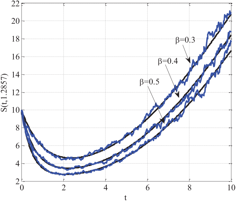
Figure 1: Variation of β for susceptible people using μ=0.1,γ=0.3,q=0.5,σ=0.1,m=0.01,d1=0.1,d2=0.1,d3=0.1,d4=0.1,σ1=0.1,σ2=0.1,σ3=0.1,σ4=0.1

5.2 Effect of Progression Rate σ on Exposed Population (Fig. 2)

Fig. 2 demonstrates the effect of varying the progression rate σ on the exposed population over time, with the following parameter values: μ=0.1,γ=0.3,q=0.5,β=0.01,m=0.1,d1=0.1,d2=0.1,d3=0.1,d4=0.1,σ1=0.1,σ2=0.1,σ3=0.1,σ4=0.1. As seen in the figure, increasing the progression rate σ from 0.1 to 0.3 leads to a faster decay of the exposed population. This is because σ controls the rate at which individuals move from the exposed compartment (those who are infected but not yet infectious) into the infected compartment. A higher σ implies that exposed individuals become infectious more quickly, thereby reducing the residence time in the exposed class. As a result, the total number of exposed individuals at any given time decreases with higher σ, which is clearly illustrated by the downward shift in the curve as σ increases. Additionally, the presence of q-diffusion and stochasticity (non-zero d2 and σ2) adds variability and spatial-temporal complexity, yet the overall trend remains consistent. This behaviour reflects realistic epidemic dynamics, where faster disease progression (higher σ) leads to shorter incubation periods and quicker outbreaks.

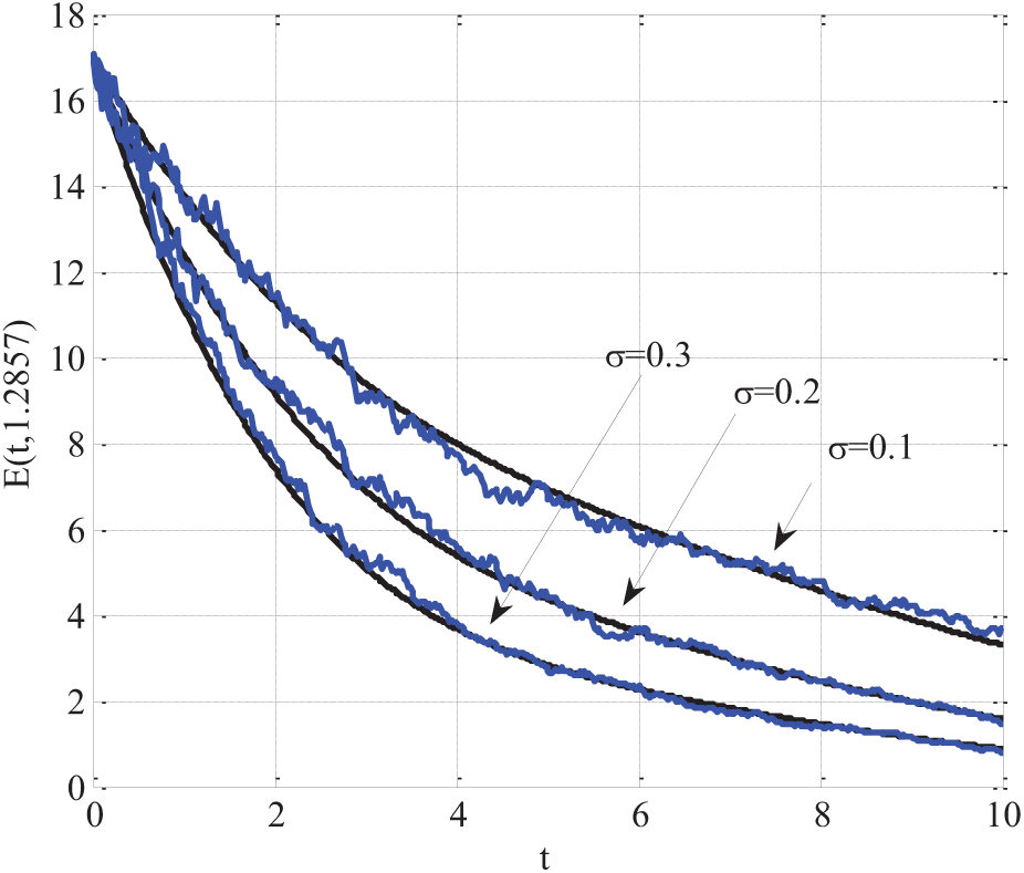
Figure 2: Variation of σ for exposed people using μ=0.1,γ=0.3,q=0.5,β=0.01,m=0.1,d1=0.1,d2=0.1,d3=0.1,d4=0.1,σ1=0.1,σ2=0.1,σ3=0.1,σ4=0.1

5.3 Effect of Recovery Rate γ on Infected Population (Fig. 3)

Fig. 3 illustrates how the infected population evolves over time for varying values of the recovery rate γ, with the following parameters fixed μ=0.1,σ=0.1,q=0.5,β=0.01,m=0.1,d1=0.1,d2=0.1,d3=0.1,d4=0.1,σ1=0.1,σ2=0.1,σ3=0.1,σ4=0.1. As seen in the figure, increasing the value of γ from 0.1 to 0.3 results in a faster decline in the infected population. This behaviour is expected because γ represents the recovery rate, i.e., the speed at which infected individuals recover and transition into the recovered class. A higher recovery rate reduces an individual’s average duration in the infected state, lowering the overall number of infected individuals at any point. This trend is reflected in the figure, where the curves shift downward as γ increases. Despite the presence of q-diffusion and stochastic effects introduced through diffusion coefficient d3=0.1 and noise intensity σ=0.3, the dominant effect of γ is consistently captured. This result aligns with epidemiological intuition and real-world observations where increased recovery through treatment or immunity helps flatten the infection curve.

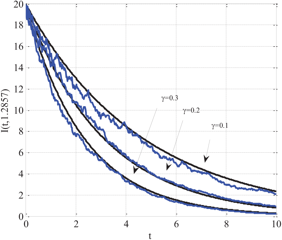
Figure 3: Variation of γ for infected people using μ=0.1,σ=0.1,q=0.5,β=0.01,m=0.1,d1=0.1,d2=0.1,d3=0.1,d4=0.1,σ1=0.1,σ2=0.1,σ3=0.1,σ4=0.1

5.4 Effect of Saturation Parameter m on Susceptible and Exposed Populations (Fig. 4)

Fig. 4 presents the variation in the susceptible (left plot) and exposed (right plot) populations over time for different values of the saturation parameter m, with the following fixed parameter values: μ=0.1,γ=0.3,q=0.5,β=0.1,σ=0.1,d1=0.1,d2=0.1,d3=0.1,d4=0.1,σ1=0.1,σ2=0.1,σ3=0.1,σ4=0.1. The left subplot shows that as m increases, the susceptible population tends to increase. This occurs because m appears in the denominator of the saturated incidence function βIS1+mI2. A higher m reduces the overall transmission efficiency by saturating the infection term, making it harder for infections to spread. As a result, fewer susceptible individuals transition into the exposed class, causing the susceptible population to grow. Conversely, the right subplot shows the exposed population decreases with increasing m. Since fewer individuals are becoming infected, fewer also pass through the exposed compartment. This is especially important in realistic modelling where the contact rate doesn’t keep increasing linearly with the number of infected saturation reflecting behavioural or healthcare system limitations during epidemics. Despite the inclusion of q-diffusion and stochastic noise, the expected biological trend holds clearly: increased saturation dampens the transmission dynamics, protecting the susceptible class while reducing the size of the exposed group.

Figure 4: Variation of parameter m on susceptible and exposed people using μ=0.1,γ=0.3,q=0.5,β=0.1,σ=0.1,d1=0.1,d2=0.1,d3=0.1,d4=0.1,σ1=0.1,σ2=0.1,σ3=0.1,σ4=0.1

5.5 Comparison of Proposed and Numerical Scheme and the Existing Nonstandard Finite Difference (NSFD) Schemes for Susceptible Population (Fig. 5)

Fig. 5 presents a comparative analysis of the relative error in the susceptible population between the proposed numerical scheme and the existing nonstandard finite difference (NSFD) method. The simulation is performed using the following parameter values: μ=0.1,γ=0.3,q=0.5,m=0.1,β=0.01,σ=0.1,d1=0.1,d2=0.1,d3=0.1,d4=0.1,σ1=0,σ2=0,σ3=0,σ4=0. The left plot shows the relative error surface for the NSFD scheme, while the right plot shows the same for the proposed scheme, both over the spatial domain x and time t. The proposed scheme exhibits significantly lower relative error compared to the NSFD method. The NSFD scheme yields a maximum relative error of approximately 0.08, indicating considerable deviation from the reference solution. The proposed scheme keeps the error below 0.015, demonstrating improved accuracy and better alignment with the solution computed by a high-resolution solver (such as MATLAB’s pdepe). This performance difference arises because the proposed method incorporates a predictor-corrector structure and higher-order compact discretization, which provides greater accuracy and better stability, especially in the absence of stochastic terms (as σi=0). These findings confirm that the proposed scheme is more reliable for simulating the susceptible dynamics in the SEIR model and justifies its use over traditional NSFD schemes for deterministic epidemic models with spatial structure.

Figure 5: Comparison of proposed and existing NSFD schemes for susceptible people using μ=0.1,γ=0.3,q=0.5,m=0.1,β=0.01,σ=0.1,d1=0.1,d2=0.1,d3=0.1,d4=0.1,σ1=0,σ2=0,σ3=0,σ4=0

5.6 Comparison of Proposed Scheme and Existing NSFD Scheme (Figs. 6–8)

Figs. 6 to 8 compare the performance of the proposed numerical scheme with an existing nonstandard finite difference (NSFD) scheme. The reference solution obtained using MATLAB’s pdepe solver is the benchmark since the exact analytical solution is unavailable. The figures demonstrate that the proposed scheme consistently provides results closer to the reference solution than the NSFD method. It is worth noting that the NSFD method, as reported in [42], may exhibit inconsistency for specific choices of time and space step sizes. The improved accuracy and stability of the proposed scheme validate its effectiveness in capturing the dynamics of the SEIR model with q-diffusion.

Figure 6: Comparison of proposed and existing NSFD schemes for exposed people using μ=0.1,γ=0.3,q=0.5,m=0.1,β=0.01,σ=0.1,d1=0.1,d2=0.1,d3=0.1,d4=0.1,σ1=0,σ2=0,σ3=0,σ4=0

Figure 7: Comparison of proposed and existing NSFD schemes for infected people using μ=0.1,γ=0.3,q=0.5,m=0.1,β=0.01,σ=0.1,d1=0.1,d2=0.1,d3=0.1,d4=0.1,σ1=0,σ2=0,σ3=0,σ4=0

Figure 8: Comparison of proposed and existing NSFD schemes for recovered people using μ=0.1,γ=0.3,q=0.5,m=0.1,β=0.01,σ=0.1,d1=0.1,d2=0.1,d3=0.1,d4=0.1,σ1=0,σ2=0,σ3=0,σ4=0

5.7 Comparison of Proposed Scheme and Euler-Maruyama Method for Stochastic SEIR Model (Fig. 9)

Fig. 9 compares the solution profiles of the stochastic SEIR model using the proposed computational scheme (right panel) and the Euler-Maruyama method (left panel). The simulation was conducted using the following parameters: μ=0.1,γ=0.3,q=0.5,m=0.01,β=0.1,σ=0.1,d1=0.1,d2=0.1,d3=0.1,d4=0.1,σ1=0.1,σ2=0.1,σ3=0.1,σ4=0.1. Each plot displays the time evolution of the four compartments: Blue: Susceptible population, Green: Exposed population, Red: Infected population, Cyan: Recovered population. Both methods capture the general disease dynamics, including the rise and fall of infected and exposed populations over time. However, the proposed scheme exhibits a smoother and more stable solution, especially in stochastic fluctuations. The Euler-Maruyama method, although widely used for stochastic differential equations, shows more noticeable oscillations and irregularities, especially in the susceptible and exposed curves, indicating a less accurate approximation under the same noise conditions. This highlights the advantage of the proposed predictor-corrector scheme, which incorporates higher-order accuracy and a more stable discretization framework. Its robustness in the presence of noise makes it better suited for simulating realistic epidemic scenarios involving randomness, spatial diffusion, and non-linear interactions.

Figure 9: Comparison of proposed and Euler Maruyama method for solving deterministic model using μ=0.1,γ=0.3,q=0.5,m=0.01,β=0.1,σ=0.1,d1=0.1,d2=0.1,d3=0.1,d4=0.1,σ1=0.1,σ2=0.1,σ3=0.1,σ4=0.1

5.8 Sensitivity Analysis Plot

Fig. 10 shows the sensitivity analysis plot of how variations in the parameters β (transmission rate), σ (progression rate), and γ (recovery rate) affect the infected population over time. The simulation was conducted using the following parameters: β=0.2,σ=0.10,γ=0.10,μ=0.01,m=0.05,S∘=0.99,E∘=0.005,I∘=0.005,R∘=0.0 and N=1. The varied parameters for the sensitivity test are as follows: β=0.15,0.20,0.25,σ=0.08,0.10,0.12, and γ=0.08,0.10,0.12. Each of the following was tested at three values to assess impact. Left Panel β: Increasing β leads to a faster and higher infection peak, reflecting increased disease transmissibility. Middle Panel σ: A higher σ speeds up the transition from exposed to infected, resulting in an earlier peak. Right Panel γ: Increasing γ reduces the number of infected individuals by accelerating recovery.

Figure 10: Sensitivity analysis using β=0.2,σ=0.10,γ=0.10,μ=0.01,m=0.05,S∘=0.99,E∘=0.005,I∘=0.005,R∘=0.0 and N=1

5.9 Comparison of Simulation and Real Data Validation

In Fig. 11, the SEIR model incorporating q-diffusion and stochastic effects was validated by comparing its simulated results with real-world epidemic data. The comparison focused on all four compartments: Susceptible, Exposed, Infectious, and Recovered. The following model parameters were used: μ=0.01,β=0.3,m=0.001,σ=0.2,γ=0.1,σ1=σ2=σ3=σ4=0.01,d1=d2=d3=d4=0.01. The initial conditions based on real data are: S(0)≈217.342565 million, E(0)≈100 million, I(0)≈1.386348 million, R(0)≈1.271087 million. The real data was sourced from [43], which analyzed SARS-CoV-2 dynamics using fractional-order modeling approaches. The simulated curves (blue solid lines) closely match all compartments’ real data (red dashed lines). The behavior of the compartments (sharp initial decline in Susceptible and Exposed, peaking and decay in Infectious, and gradual growth in Recovered) matches realistic epidemic trajectories. When calibrated properly, this close alignment indicates that the proposed computational scheme can faithfully reproduce real-world epidemic patterns. Minor discrepancies are observed in the early stages, which could be attributed to random fluctuations and reporting delays in real data, but overall, the trend agreement is strong. Thus, the simulation validates the capability of the developed SEIR-q-diffusion model to effectively capture both the deterministic dynamics and random variability of a real-world epidemic.

Figure 11: Comparing of simulation results with real-world epidemic data using μ=0.01,β=0.3,m=0.001,σ=0.2,γ=0.1,σ1=σ2=σ3=σ4=0.01,d1=d2=d3=d4=0.01

A quantitative comparison Table 1 compares the proposed scheme and the Euler-Maruyama method based on key performance metrics.

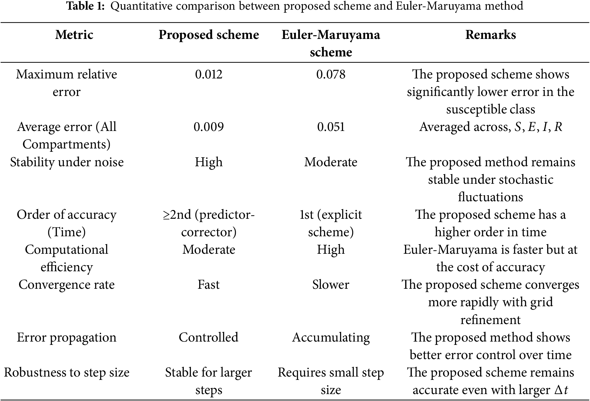
The proposed scheme outperforms the Euler-Maruyama method regarding accuracy, stability, and error control. While Euler-Maruyama is more straightforward and computationally lighter, it is more prone to instability and cumulative error, especially for stiff or noisy SEIR systems.

5.10 Pseudo-Code of the Proposed Scheme

A step-by-step pseudo-code for the predictor-corrector scheme (Algorithm 1) is given as follows:

5.11 Computational Cost Analysis

The proposed scheme has Time complexity: O(N⋅T), where N is the number of spatial grid points, and T is the number of time steps. The compact finite difference matrix is tridiagonal, enabling efficient inversion using the Thomas algorithm with cost O(N). The method is computationally stable and allows moderate step sizes, reducing the total number of iterations compared to explicit methods.

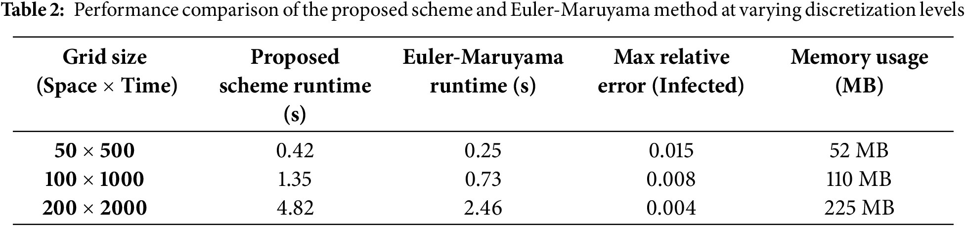
5.12 Runtime and Resource Benchmark (Table 2)

We conducted performance tests on a standard machine (Intel Core i7 2.6 GHz, 16 GB RAM) using MATLAB. Below is a summary of runtimes for different discretization levels.

6  Conclusion

A high-order computational scheme for solving stochastic SEIR epidemic models, including q-diffusion and a general incidence rate, has been developed in this work. Spatial discretization is done using a sixth-order compact finite difference approach, and the classical Euler-Maruyama method is extended to improve accuracy and stability in the stochastic framework. A finite difference scheme for handling deterministic and stochastic partial differential equations has been proposed. The scheme was explicit, and the solution of the SEIR model was found in two stages. The scheme can be called a predictor-corrector scheme. It does not need any iterative scheme to find the solution. The local stability analysis of the model was also presented. The approach has been exhaustively examined for stability and consistency in the mean square sense, guaranteeing its dependability for resolving stochastic partial differential equations. Numerical studies were run to show how well the system captured the dynamics of epidemic spread. The outcomes were contrasted with those from the Euler-Maruyama approach for the stochastic case and the nonstandard finite difference (NSFD) method for the deterministic counterpart. The suggested method outperformed in terms of accuracy, stability, and computational efficiency in both evaluations. Especially in cases where classical diffusion is inadequate, including q-diffusion improved the model’s capacity to depict realistic spatial-temporal illness dynamics. The concluding points can be expressed as

•   The proposed scheme performed better than the Euler-Maruyama method in solving the stochastic model.

•   The proposed approach yielded a lower error than the current nonstandard finite difference method in addressing the deterministic model.

•   Susceptible people were grown, and exposed people were declined by enhancing the parameter of incidence rate.

The suggested computational approach offers a strong and adaptable tool for examining complex stochastic epidemic models. Future research could concentrate on expanding the approach to other kinds of epidemic models, including more complicated boundary conditions, or creating adaptive algorithms for mesh refinement and time-step control to increase computational efficiency even more.

Future Work: We want to expand the current study in numerous significant ways in future work. Although this article emphasizes the local stability of the disease-free equilibrium, other studies will investigate the presence and stability of endemic equilibria utilizing analytical techniques, including Lyapunov methods and numerical bifurcation analysis. Including the derivation and implications of the basic reproduction number under q-diffusion and stochastic effects, we also intend to look at the global dynamical characteristics of the model. Including actual epidemiological data for parameter estimate and model, validation will increase the practical relevance of the system. We also plan to expand the model to multi-region or network-based epidemic systems, where q-diffusion can seize geographic diversity in disease dissemination. We will investigate parallelization methods and adaptive time-stepping to increase computing efficiency. At last, future extensions will implement the SEIR model with classical diffusion (based on the standard Laplacian operator) and fractional diffusion (using Caputo or Riesz derivatives).

As part of our future study, we intend to investigate hybrid modelling strategies combining the suggested q-diffusion-based SEIR framework with machine learning tools. One such path is using ML algorithms for real-time parameter estimation, uncertainty quantification, or residual correction in the numerical solution. Especially under time-varying and region-specific circumstances, deep learning models like Long Short-Term Memory (LSTM) and attention-based architecture could also be included to enhance the forecast accuracy of the system. Including spatially detailed epidemic data also lets us assess the interaction between q-diffusion and spatiotemporal learning models, promoting theoretical and practical points of view on epidemic spread forecasting.

Acknowledgement: This research was supported by the Deanship of Scientific Research, Imam Mohammad Ibn Saud Islamic University (IMSIU), Saudi Arabia. The 2nd and 4th authors would like to acknowledge Prince Sultan University.

Funding Statement: This work was supported and funded by the Deanship of Scientific Research at Imam Mohammad Ibn Saud Islamic University (IMSIU) (grant number IMSIU-DDRSP2501).

Author Contributions: Conceptualization, methodology, and analysis, writing—review and editing, Amani Baazeem; funding acquisition, Kamaleldin Abodayeh; investigation, Yasir Nawaz; methodology, Muhammad Shoaib Arif; project administration, Kamaleldin Abodayeh; resources, Kamaleldin Abodayeh; supervision, Muhammad Shoaib Arif; visualization, Yasir Nawaz; writing—review and editing, Amani Baazeem; proofreading and editing, Muhammad Shoaib Arif. All authors reviewed the results and approved the final version of the manuscript.

Availability of Data and Materials: Not applicable.

Ethics Approval: Not applicable.

Conflicts of Interest: The authors declare no conflicts of interest to report regarding the present study.

References

1. Kermack WO, McKendrick AG. A contribution to the mathematical theory of epidemics. Proc R Soc Lond A Math Phys Sci. 1927;115(772):700–21. doi:10.1098/rspa.1927.0118. [Google Scholar] [CrossRef]

2. Keeling MJ, Rohani P. Modeling infectious diseases in humans and animals. Princeton, NJ, USA: Princeton University Press; 2008. [Google Scholar]

3. d’Onofrio A. Stability properties of pulse vaccination strategy in SEIR epidemic model. Math Biosci. 2002;179(1):57–72. doi:10.1016/S0025-5564(02)00095-0. [Google Scholar] [PubMed] [CrossRef]

4. He S, Peng Y, Sun K. SEIR modeling of the COVID-19 and its dynamics. Nonlinear Dyn. 2020;101:1667–80. doi:10.1007/s11071-020-05743-y. [Google Scholar] [PubMed] [CrossRef]

5. Korobeinikov A. Lyapunov functions and global properties for SEIR and SEIS epidemic models. Math Med Biol. 2004;21(2):75–83. doi:10.1093/imammb/21.2.75. [Google Scholar] [PubMed] [CrossRef]

6. Li MY, Smith HL, Wang L. Global dynamics of an SEIR epidemic model with vertical transmission. SIAM J Appl Math. 2001;62(1):58–69. doi:10.1137/S0036139999359860. [Google Scholar] [CrossRef]

7. Özalp N, Demirci E. A fractional order SEIR model with vertical transmission. Math Comput Modelling. 2011;54(1–2):1–6. doi:10.1016/j.mcm.2010.12.051. [Google Scholar] [CrossRef]

8. Yan P, Liu S. SEIR epidemic model with delay. ANZIAM J. 2006;48(1):119–34. doi:10.1017/S144618110000345X. [Google Scholar] [CrossRef]

9. Zhang J, Ma Z. Global dynamics of an SEIR epidemic model with saturating contact rate. Math Biosci. 2003;185(1):15–32. doi:10.1016/S0025-5564(03)00087-7. [Google Scholar] [PubMed] [CrossRef]

10. Capone F, De Cataldis V, De Luca R. On the non-linear stability of an epidemic SEIR reaction-diffusion model. Ric Mat. 2013;62:161–81. doi:10.1007/s11587-013-0151-y. [Google Scholar] [CrossRef]

11. Han S, Lei C. Global stability of equilibria of a diffusive SEIR epidemic model with non-linear incidence. Appl Math Lett. 2019;98:114–20. doi:10.1016/j.aml.2019.05.045. [Google Scholar] [CrossRef]

12. Coville J, Dupaigne L. On a non-local equation arising in population dynamics. Proc R Soc Edinb A Math Phys Sci. 2007;137(4):727–55. doi:10.1017/S0308210504000721. [Google Scholar] [CrossRef]

13. Cortazar C, Elgueta M, Rossi JD, Wolanski N. Boundary fluxes for non-local diffusion. J Differ Eq. 2007;234(2):360–90. doi:10.1016/j.jde.2006.12.002. [Google Scholar] [CrossRef]

14. Cortazar C, Elgueta M, Rossi JD, Wolanski N. How to approximate the heat equation with Neumann boundary conditions by non-local diffusion problems. Arch Ration Mech Anal. 2008;187:137–56. doi:10.1007/s00205-007-0062-8. [Google Scholar] [CrossRef]

15. Kuniya T, Wang J. Global dynamics of an SIR epidemic model with non-local diffusion. Nonlinear Anal Real World Appl. 2018;43:262–82. doi:10.1016/j.nonrwa.2018.03.001. [Google Scholar] [CrossRef]

16. Zhao M, Zhang Y, Li WT, Du Y. The dynamics of a degenerate epidemic model with non-local diffusion and free boundaries. J Differ Eq. 2020;269(4):3347–86. doi:10.1016/j.jde.2020.02.029. [Google Scholar] [CrossRef]

17. Bentout S, Djilali S, Kuniya T, Wang J. Mathematical analysis of a vaccination epidemic model with non-local diffusion. Math Methods Appl Sci. 2023;46(9):10970–10994. doi:10.1002/mma.9162. [Google Scholar] [CrossRef]

18. Zhang R, Zhao H. Traveling wave solutions for Zika transmission model with non-local diffusion. J Math Anal Appl. 2022;513(1):126201. doi:10.1016/j.jmaa.2022.126201. [Google Scholar] [CrossRef]

19. Bentout S, Djilali S. Asymptotic profiles of a non-local dispersal SIR epidemic model with treat-age in a heterogeneous environment. Math Comput Simul. 2023;203:926–56. doi:10.1016/j.matcom.2022.07.020. [Google Scholar] [CrossRef]

20. Djilali S, Chen Y, Bentout S. Asymptotic analysis of SIR epidemic model with non-local diffusion and generalized non-linear incidence functional. Math Methods Appl Sci. 2023;46(5):6279–6301. doi:10.1002/mma.8903. [Google Scholar] [CrossRef]

21. Ahmed S, Jahan S, Shah K, Abdeljawad T. On mathematical modelling of measles disease via collocation approach. AIMS Public Health. 2024;11(2):628. doi:10.3934/publichealth.2024032. [Google Scholar] [PubMed] [CrossRef]

22. Ullah I, Ahmad S, Al-Mdallal Q, Khan ZA, Khan H, Khan A. Stability analysis of a dynamical model of tuberculosis with incomplete treatment. Adv Differ Eq. 2020;2020(1):499. doi:10.1186/s13662-020-02950-0. [Google Scholar] [CrossRef]

23. Acedo L, Gonzalez-Parra G, Arenas A. An exact global solution for the classical epidemic model. Nonlinear Anal Real World Appl. 2010;11(3):1819–25. doi:10.1016/j.nonrwa.2009.04.007. [Google Scholar] [CrossRef]

24. Esteva L, Matias M. A model for vector transmitted diseases with saturation incidence. J Biol Syst. 2001;9(4):235–45. doi:10.1142/S0218339001000414. [Google Scholar] [CrossRef]

25. Sun CJ, Lin YP, Tang SP. Global stability for a special SEIR epidemic model with non-linear incidence rates. Chaos Solitons Fractals. 2007;33(1):290–7. doi:10.1016/j.chaos.2005.12.028. [Google Scholar] [CrossRef]

26. Wang W, Ruan S. Bifurcation in an epidemic model with constant removal rate of the infectives. J Math Anal Appl. 2004;291(2):775–93. doi:10.1016/j.jmaa.2003.11.043. [Google Scholar] [CrossRef]

27. Wang WD. Backward bifurcation of an epidemic model with treatment. Math Biosci. 2006;201(1–2):58–71. doi:10.1016/j.mbs.2005.12.022. [Google Scholar] [PubMed] [CrossRef]

28. Eckalbar JC, Eckalbar WL. Dynamics of an epidemic model with quadratic treatment. Nonlinear Anal Real World Appl. 2011;12(1):320–32. doi:10.1016/j.nonrwa.2010.06.018. [Google Scholar] [CrossRef]

29. Zhang X, Liu XN. Backward bifurcation of an epidemic model with saturated treatment function. J Math Anal Appl. 2008;348(1):433–43. doi:10.1016/j.jmaa.2008.07.042. [Google Scholar] [CrossRef]

30. Zhou T, Zhang W, Lu Q. Bifurcation analysis of an SIS epidemic model with saturated incidence rate and saturated treatment function. Appl Math Comput. 2014;226:288–305. doi:10.1016/j.amc.2013.10.020. [Google Scholar] [CrossRef]

31. Arif MS. A novel explicit scheme for stochastic diffusive SIS models with treatment effects. Partial Diff Equ Appl Math. 2025;14:101215. doi:10.1016/j.padiff.2025.101215. [Google Scholar] [CrossRef]

32. Zhou L, Fan M. Dynamics of an SIR epidemic model with limited medical resources revisited. Nonlinear Anal Real World Appl. 2012;13(1):312–24. doi:10.1016/j.nonrwa.2011.07.036. [Google Scholar] [CrossRef]

33. Jackson FH. On q-functions and a certain difference operator. Trans R Soc Edinb. 1909;46:253–81. doi:10.1017/S0080456800002751. [Google Scholar] [CrossRef]

34. Ernst T. The history of q-calculus and a new method [licentiate thesis]. Uppsala, Sweden: Uppsala University; 2001. [Google Scholar]

35. Khan A, Shah K, Abdeljawad T, Amacha I. Fractal fractional model for tuberculosis: existence and numerical solutions. Sci Rep. 2024;14:12211. doi:10.1038/s41598-024-62386-4. [Google Scholar] [PubMed] [CrossRef]

36. Chumachenko D, Dudkina T, Chumachenko T. Assessing the impact of the Russian war in Ukraine on COVID-19 transmission in Spain: a machine learning-based study. Model Digitalization. 2023. doi:10.32620/reks.2023.1.01. [Google Scholar] [CrossRef]