
 Submit a Paper
 Propose a Special lssue
 Open Access
REVIEW

Advanced Signal Processing and Modeling Techniques for Automotive Radar: Challenges and Innovations in ADAS Applications
1 Department of Electronics and Communication Engineering, Sikkim Manipal Institute of Technology, Majhitar, Sikkim Manipal University, Gangtok, 737136, Sikkim, India
2 Department of Computer Science and Engineering, Sikkim Manipal Institute of Technology, Majhitar, Sikkim Manipal University, Gangtok, 737136, Sikkim, India
3 Department of Electronics and Communication Engineering, Indian Institute of Information Technology, Kalyani, 741235, West Bengal, India
4 Department of Electrical and Electronics Engineering, Faculty of Engineering, University of Lagos, Akoka, Lagos, 100213, Nigeria
5 Bachelor’s Program of Artificial Intelligence and Information Security, Fu Jen Catholic University, 510 Zhongzheng Road, New Taipei City, 242062, Taiwan
* Corresponding Authors: Samarendra Nath Sur. Email: ; Chun-Ta Li. Email:
# These authors contributed equally to this work
Computer Modeling in Engineering & Sciences 2025, 144(1), 83-146. https://doi.org/10.32604/cmes.2025.067724
Received 10 May 2025; Accepted 02 July 2025; Issue published 31 July 2025
 View Full Text
 Download PDF
Abstract
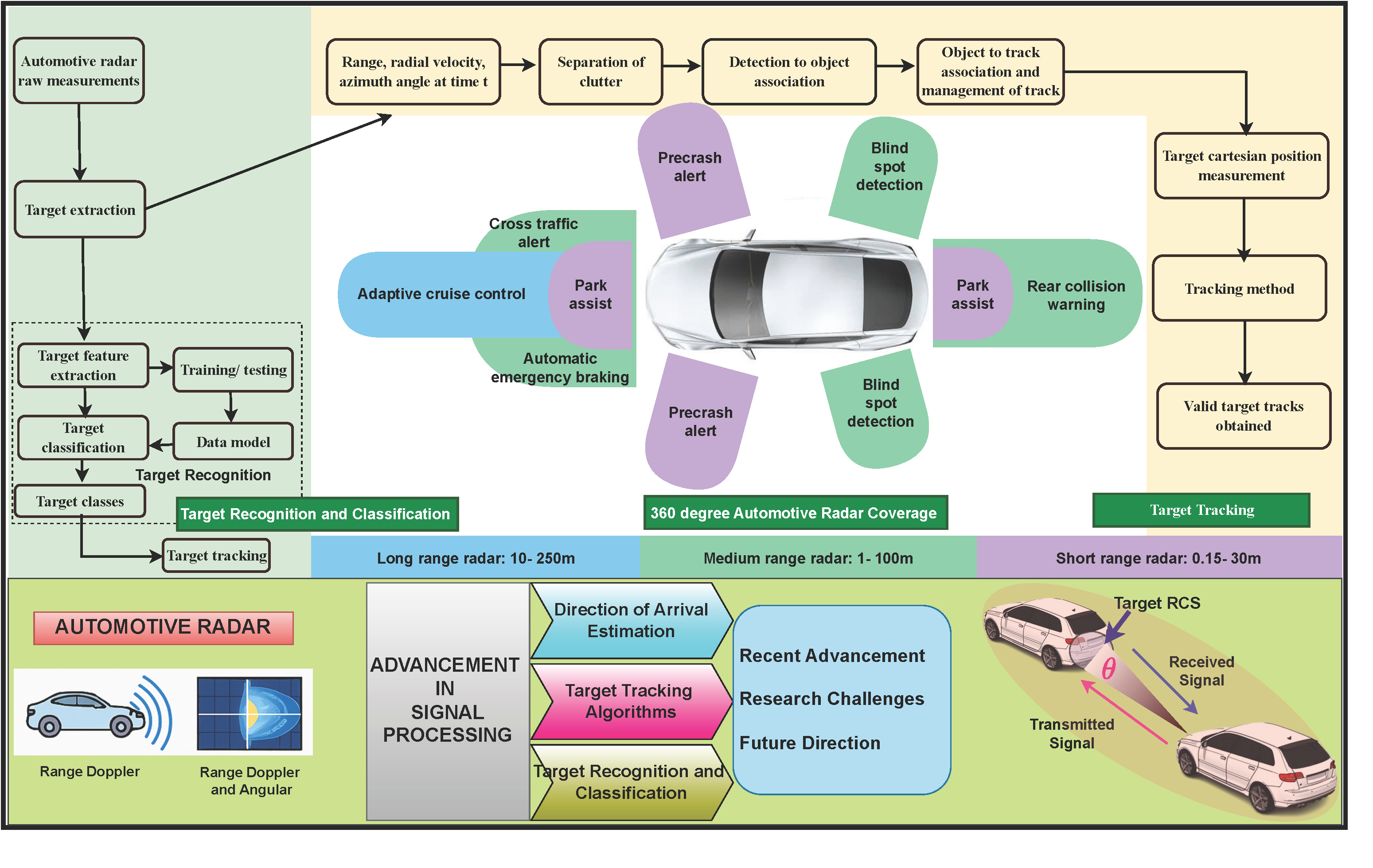
Automotive radar has emerged as a critical component in Advanced Driver Assistance Systems (ADAS) and autonomous driving, enabling robust environmental perception through precise range-Doppler and angular measurements. It plays a pivotal role in enhancing road safety by supporting accurate detection and localization of surrounding objects. However, real-world deployment of automotive radar faces significant challenges, including mutual interference among radar units and dense clutter due to multiple dynamic targets, which demand advanced signal processing solutions beyond conventional methodologies. This paper presents a comprehensive review of traditional signal processing techniques and recent advancements specifically designed to address contemporary operational challenges in automotive radar. Emphasis is placed on direction-of-arrival (DoA) estimation algorithms such as Bartlett beamforming, Minimum Variance Distortionless Response (MVDR), Multiple Signal Classification (MUSIC), and Estimation of Signal Parameters via Rotational Invariance Techniques (ESPRIT). Among these, ESPRIT offers superior resolution for multi-target scenarios with reduced computational complexity compared to MUSIC, making it particularly advantageous for real-time applications. Furthermore, the study evaluates state-of-the-art tracking algorithms, including the Kalman Filter (KF), Extended KF (EKF), Unscented KF, and Bayesian filter. EKF is especially suitable for radar systems due to its capability to linearize nonlinear measurement models. The integration of machine learning approaches for target detection and classification is also discussed, highlighting the trade-off between the simplicity of implementation in K-Nearest Neighbors (KNN) and the enhanced accuracy provided by Support Vector Machines (SVM). A brief overview of benchmark radar datasets, performance metrics, and relevant standards is included to support future research. The paper concludes by outlining ongoing challenges and identifying promising research directions in automotive radar signal processing, particularly in the context of increasingly complex traffic scenarios and autonomous navigation systems.Graphic Abstract
Keywords
Next-generation vehicles are equipped with Advanced Driver Assistance Systems (ADAS) designed to enhance driving safety while ensuring a safe and stress-free journey [1]. According to the report provided by the World Health Organization (WHO), road traffic accidents resulted in approximately 1.19 million fatalities in 2023 [2]. The high rate of casualties, significant financial losses, and the growing demand for intelligent safety systems have driven manufacturers to advance autonomous driving technologies [3].
In fully automated vehicles, human drivers are replaced by intelligent systems responsible for both sensing and decision-making. The ADAS framework integrates multiple sensors, including radar, LiDAR, and cameras, to ensure reliable vehicle performance and improve driver assistance. Among these, radar is particularly effective for detecting the range and velocity of objects, processing data efficiently, and operating under challenging weather conditions. LiDAR offers high-range accuracy and superior angular resolution but is susceptible to adverse weather conditions and interference [4]. Cameras provide color distinction, high angular resolution, and accurate target classification but cannot measure velocity and range, and their performance is compromised in low-light and adverse weather conditions [5]. Given these limitations, automotive radar is the primary sensing modality for automated vehicles [6].
Radars were developed as military tools during and after World War II [7]. Over time, the applications expanded to include air traffic control, weather Radars, ground-penetrating radars, guided missile target locating systems, and more. Automotive Radar applications were first developed in the early 1970s as part of a German research program (NTO 49) aimed at reducing road accidents [8]. In recent times, the Euro New Car Assessment Program (NCAP) for European road safety requires Adaptive Cruise Control (ACC), Automotive Emergency Braking (AEB), Lane Change Assist (LCA), etc. In [9], a semi-physical Radar modeling technique has been adopted to observe the accuracy of the probability density function of Radar data and the Radar Cross Section (RCS) values obtained are similar to the values for global vehicle target validation of NCAP.
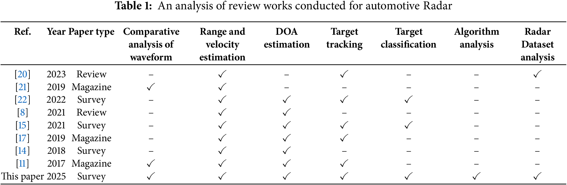
Automotive Radars are mostly used in the 24 and 77 GHz ranges of the frequency spectrum. A 4 GHz bandwidth, improved range resolution, proper Doppler sensitivity that leads to velocity resolution, and a reduced antenna aperture, which is useful for fitting on vehicles, are the important advantages of using the 77–81 GHz frequency band. Automotive Radars operating in the 24 GHz frequency band are used for ultra-wideband applications. An arrangement of planar grid antenna array for this Radar improves the antenna gain and impedance bandwidth [10]. Performance criteria of automotive Radar include target resolution, range resolution, dynamic range in terms of velocity, and direction of arrival of the received signal. Fig. 1 represents a 360 degree surround sensing by Radar scenario of an autonomous car [11]. A Long Range Radar (LRR) having a range of 10–250 m is mounted in front of a vehicle and is suitable for ACC [12]. Medium Range Radars (MRR) with a range of 1–100 m are fitted on the front and rear sides and are applicable for Lane Change Assistance and warning of rear collisions. Short-range radars (SRRs) with a range of 0.15–30 m are fitted at the four corners of a car and are applicable for parking assist, obstacle detection, etc. [13]. The various radars, along with their respective functions, are depicted in Fig. 1.
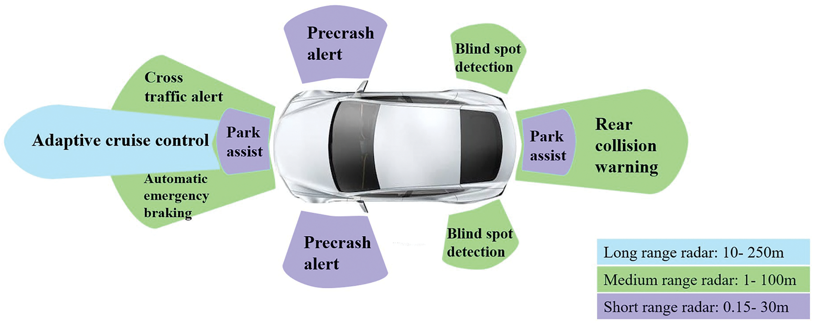
Figure 1: Vehicle in 360° Automotive radar coverage for collision avoidance
Automotive radar systems are generally composed of three main components: the transmitter, the receiver, and the signal processing subsystem. On the transmitter side, the antenna operates using a frequency-modulated continuous wave (FMCW) chirp waveform [14]. Signal processing at this stage involves generating a series of up-and-down chirps using a frequency-generating circuit, which are then transmitted via the antenna. The antenna radiates power that is regulated by design constraints, thereby influencing the transmitter architecture. Notably, the maximum detectable range is proportional to the square root of the transmitted power. The transmitter typically consists of a waveform generator, an upconverter, and a power amplifier. The waveform generator produces a predefined signal, either continuous or pulsed, at an intermediate frequency (IF). This signal is then converted to a higher radio frequency (RF) via the up-converter and subsequently amplified using a power amplifier with adjustable gain. The transmitted signal reflects off-targets and returns to the radar system, where it is received and mixed with a copy of the transmitted signal, resulting in a beat frequency. The receiver must maximize the signal-to-noise ratio (SNR) to suppress or eliminate unwanted signals and clutter. To achieve this, the receiver includes a low-noise amplifier (LNA) and a down-converter, which utilizes a local oscillator to convert the RF signal back to IF.
The signal processing subsystem plays a crucial role in extracting range and velocity information. It involves applying a Fourier Transform to the beat frequencies to perform range estimation and analyzing the Doppler-induced phase shifts across multiple chirps to measure target velocity. This is typically accomplished through a two-stage Fast Fourier Transform (FFT): a fast-time FFT for range estimation and a slow-time FFT for Doppler estimation, followed by beamforming techniques [15,16]. Direction of arrival (DOA) estimation is performed using array processing techniques, such as digital beamforming. Based on the extracted information, a target list is generated, enabling detection and analysis of target parameters. This is followed by stationary and dynamic target processing, wherein stationary targets undergo classification while moving targets are subject to tracking and classification. A high-level block diagram of the automotive radar signal processing chain is presented in Fig. 2.
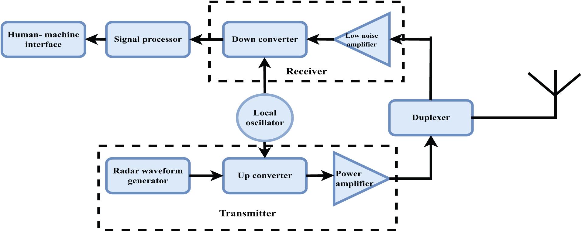
Figure 2: Automotive radar processing system
Automotive Radar operational hurdles [17]:
1. In urban environments, automotive radar systems are significantly affected by multipath propagation, which arises from reflections of various surrounding objects such as pedestrians, vehicles, road infrastructure, and animals. These objects exhibit varying Radar Cross Section (RCS), velocities, and movement patterns, necessitating high precision in target detection, localization, tracking, and classification. Multipath interference can introduce false target detections, which can adversely impact overall radar performance. Mitigating these effects requires applying advanced signal processing techniques, which, in turn, increases the computational complexity of the system.
2. In automotive radar systems, any object above the road surface that interferes with signal reception is classified as clutter. Clutter originating from nearby obstacles significantly influences the required suppression levels of antenna sidelobes, particularly in the elevation plane. Echoes received through sidelobes can, in some cases, exhibit greater power than returns from weaker targets captured by the main lobe, potentially causing signal interference. Consequently, the design of radar detectors capable of accurately identifying weak targets in the presence of strong clutter is essential to ensure robust and reliable system performance.
3. Automotive radar systems also encounter significant challenges due to interference, which can be broadly classified into three categories: self-interference, intra-vehicle cross-interference, and inter-vehicle cross-interference. Self-interference arises from reflections of the radar signal off the vehicle’s structure, such as the frame or radome, which can hinder the operation of SRR systems. Intra-vehicle cross-interference occurs when multiple radar units installed on the same vehicle have overlapping fields of view, leading to mutual signal disruption. Inter-vehicle cross-interference is induced by radar systems mounted on other vehicles in close proximity, with the severity of interference determined by the relative distance between vehicles and the characteristics of their transmitted waveforms. Addressing these interference sources is critical for maintaining the integrity and reliability of radar-based perception systems in automotive environments.
As stated before, the application areas of automotive radars include ACC, AEB, etc., which further help in the process of vehicle automation. With this ADAS system, the Society of Automotive Engineers (S.A.E.) and the National Highway Traffic Safety Administration have thus standardized six levels of autonomous driving [18]:
1. Level 0: The driver undertakes driving tasks without any automation
2. Level 1: Automation system takes over either steering or acceleration, but the driver monitors, like the Cross Traffic Assist function
3. Level 2: The system takes over functions like adaptive cruise control and brake assist, but the driver still monitors.
4. Level 3: Most tasks are automated, and the system informs the driver when necessary.
5. Level 4: The whole driving task is to be automated and the human driver is to be notified only in undefined cases.
6. Level 5: Fully automated with no driver intervention.
Fig. 3 presents the evolution of automotive Radar for ADAS applications and economic development [19].
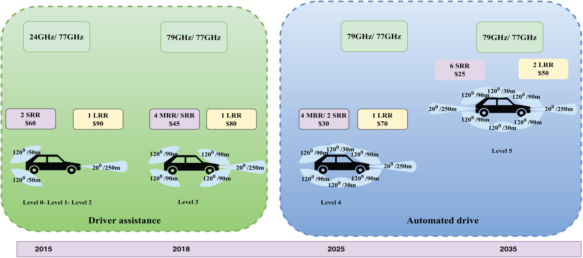
Figure 3: Evolution of automotive radar for ADAS [19]
The contributions of this paper include:
1. A comprehensive overview of automotive radar signal processing techniques, including range and velocity estimation, has been presented. Additionally, a comparative analysis of various waveform types has been conducted, highlighting their respective advantages and limitations in the context of automotive applications. The study also examines different forms of interference encountered in radar systems. Furthermore, a comparative summary of existing review articles on automotive radar offers insight into the current state of research and emerging trends in the field.
2. A detailed analysis of target detection methods and various DOA estimation algorithms has been presented. Comparative evaluations of these algorithms are provided in tabular form, highlighting their respective advantages and limitations. This analysis facilitates a clearer understanding of the trade-offs involved in selecting appropriate DOA estimation techniques for automotive radar applications.
3. Various target tracking algorithms, as proposed in key contributions from existing literature, have been discussed. A comparative table is also included to illustrate the respective advantages and disadvantages of each algorithm, providing insight into their applicability and performance in automotive radar systems.
4. Target recognition and classification using Machine Learning (ML) algorithms has emerged as a significant area of research in automotive radar systems. Various algorithms currently under investigation have been discussed in detail, along with an analysis of their respective strengths and limitations.
5. Key research challenges in the field of automotive radar have also been outlined to support future efforts aimed at addressing these issues and advancing the state of the art.
6. To obtain the training data for the ML algorithms, a large Radar dataset is used that contains a detailed description of the surrounding environment. In this work, the publicly available important datasets are described concisely. Additionally, automotive Radar evaluation metrics and global standards are also provided.
Table 1 presents a comparison between earlier review works on signal processing techniques for automotive radars and this work.
The remainder of this paper is organized as follows: Section 2 provides an overview of automotive radar systems, including fundamental mathematical formulations and commonly used radar waveforms. Section 3 presents a detailed analysis of existing research on target detection and Direction-of-Arrival (DOA) estimation techniques. Section 4 discusses various target-tracking methods explored in the literature. Section 5 reviews recent advances in target recognition and classification approaches. Section 6 outlines the key research challenges and potential future directions in the field of automotive radar. Section 7 presents an overview of the various automotive Radar databases available publicly for further research in this field, as well as the standards and parameter evaluation metrics for automotive Radar. Finally, the paper concludes with a summary of key findings.
2 Overview of Automotive Radar
Modern automotive Radar generally applies a frequency-modulated continuous chirp waveform (FMCW), working in frequency ranges of 24 and 76–81 GHz. To detect targets, a series of signals with up chirp and down chirp is generated by a frequency-generating circuit like a phase locked loop (PLL) and transmitted using a transmit antenna [20]. This chirp waveform in the time-frequency domain is presented in Fig. 4, where the transmitted wave, received wave, and beat frequency are identified.
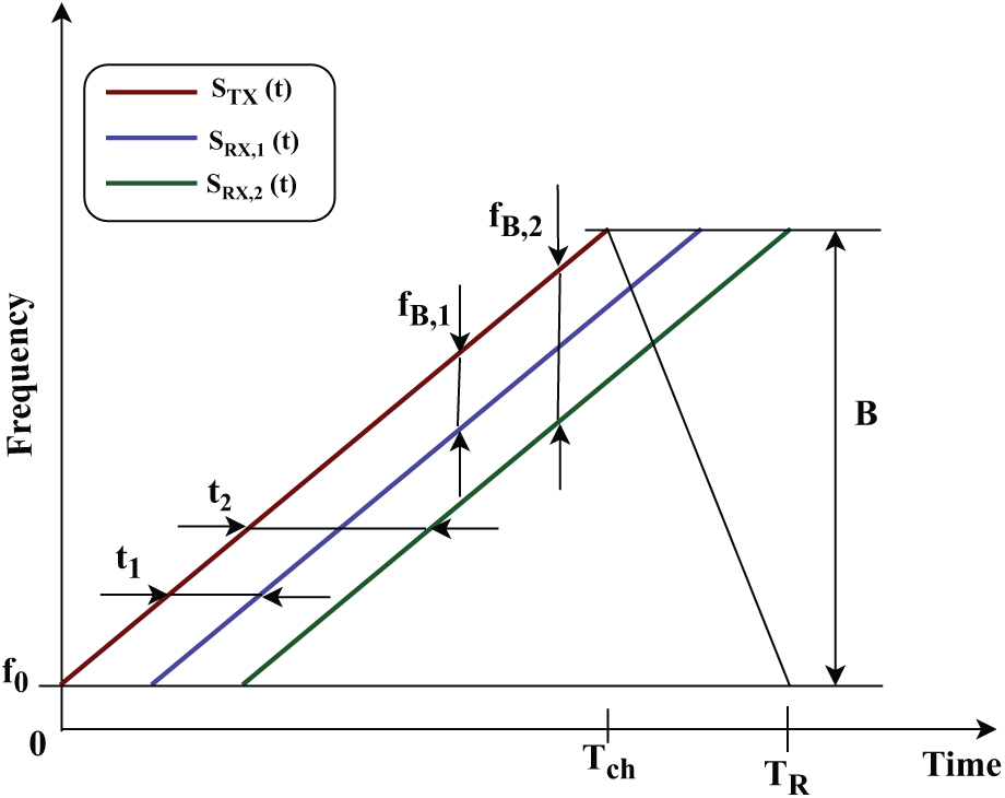
Figure 4: Time vs. frequency domain representation of FMCW radar
The transmitted signal
for,
A corresponding echo is reflected from the surroundings for each chirp incident on the targets. For simplicity, a target can be considered as a point target. The received signal is a time-delayed and attenuated form of the transmitted signal. The received signal is presented as,
where
At the receiving end, the received signal is multiplied by the transmitted signal and then filtered using a low-pass filter to get a signal having IF. The basic mathematical model to estimate the velocity and range of a desired mobile target can be derived from processing this IF frequency signal, which is shown as follows:
in which,
Using this
Whether the received signal is coming from a recent chirp or a previous one leads to ambiguity. The maximal unambiguous range can be shown as,
where
This proves that range resolution improves when bandwidth is increased.
Velocity measurement of a particular target using Radar depends on the Doppler effect. Here, two targets at equal distances but in motion in reverse directions with corresponding velocities
where
where
For the two targets considered above, the velocities are given as,
where
where
The position of a particular target is shown in a spherical coordinate system presented as (R,
Automotive radar performance is evaluated based on several metrics, including velocity resolution, range resolution, angular resolution, and target detection probability. The choice of waveform has a significant impact on these performance parameters. Radar waveforms are generally categorized into continuous wave (CW), pulsed, and modulated types. Modulated waveforms comprise FMCW, Orthogonal Frequency Division Multiplexing (OFDM), and Phase Modulated Continuous Wave (PMCW) [11]. A detailed discussion of these waveform types is provided in the following.
In a CW waveform, the transmitted and received signals are processed using a conjugate product, generating a signal corresponding to the specific target’s Doppler frequency. However, due to the continuous behavior of this waveform, measuring the delay due to the round-trip is challenging, making range resolution difficult to achieve. Typically, CW radar systems require separate antennas for transmission and reception.
The duration of a pulse and pulse repetition frequency (PRF) are used for designing this waveform with the required range and velocity estimation. For a pulsed waveform, one antenna system can be used for both transmission and reception processes. Fig. 5 presents a comparative representation of a continuous wave and a pulsed continuous wave.
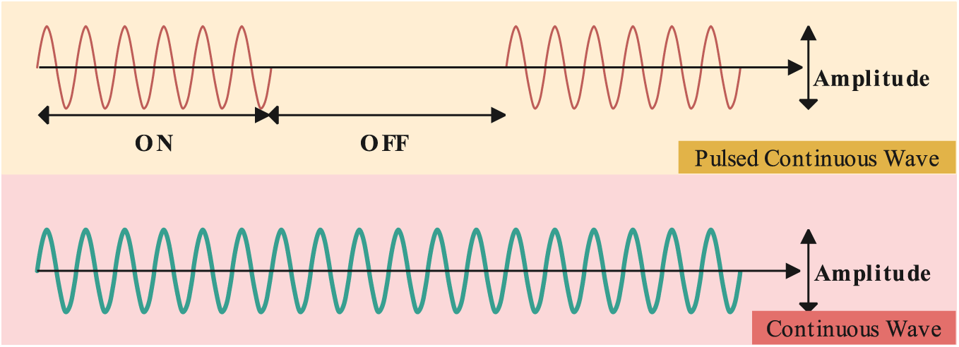
Figure 5: Representation of continuous wave and pulsed continuous wave
2.4.3 Frequency Modulated Continuous Wave
For the FMCW [23] automotive Radar, the carrier signal is modulated by the transmitter by a linear increase of the frequency over time for a predefined interval called a chirp. The main characteristic of FMCW is that the velocity and range of the target can be simultaneously estimated using the 2-dimensional (2D) FFT process. A wide sweep bandwidth improves range resolution as these factors are inversely proportional. The Doppler resolution is determined by the pulse width and the total number of pulses required for this measurement. In the Linear FMCW waveform, the beat frequency for a single mobile target can be derived after the received echo signal is combined with the signal transmitted. Thus, it is composed of a Doppler frequency shift
Here,
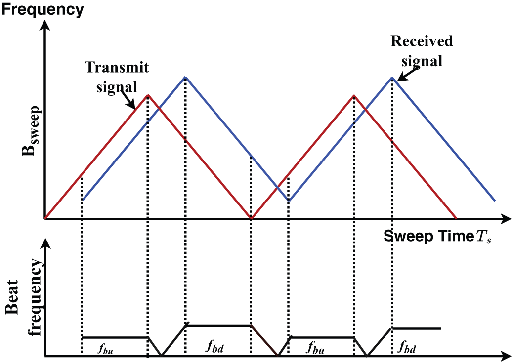
Figure 6: Beat frequency generation using chirp signal to estimate range and velocity
Two beat frequencies, one each for the upward slope
By applying the FFT on each reflected chirp, the target’s range is measured as:
After Range-FFT, another “Fourier transform”, “Doppler-FFT” is applied to obtain the velocities of multiple targets
Stepped FMCW—For this waveform, a sequence of sinusoidal signals is transmitted at distinct frequencies, and the phase shift and steady-state amplitude caused by the Radar channel at each distinct frequency are measured. The inverse discrete Fourier transformation (IDFT) measures the target range. Sparse stepped frequency waveform [24] provides lower levels of range sidelobe for the detection of weak targets. Using a sparse array interpolation method, the sidelobes are reduced, resulting in a mitigation of the likelihood of a “false alarm” during the evaluation of the target angle. Interrupted FMCW—In Interrupted FMCW, reception of target echo is allowed only when the timing signal is off. For short-range targets, the total reception time is reduced, making it difficult to detect those targets. But the effect is reversed for long-range targets. So, an arrangement needs to be made between SRR and LRR. An online learning approach based on the Thompson sampling technique can be applied to identify which FMCW waveform will be beneficial for target classification [25].
2.4.4 Fast Chirp Ramp Sequence Waveform
The advantage of a fast chirp waveform [26] over a usual FMCW waveform is that a 2D-FFT processing enables range and velocity estimation of a target accurately. To collect range information, this 2D-FFT is applied first for each chirp and then across chirps to obtain velocity information. Additionally, the beat frequency signals from targets are greater than the noise corner frequency, providing an improved SNR for detecting weak targets. An example of a fast chirp ramp sequence in the time-frequency domain is indicated in Fig. 7.
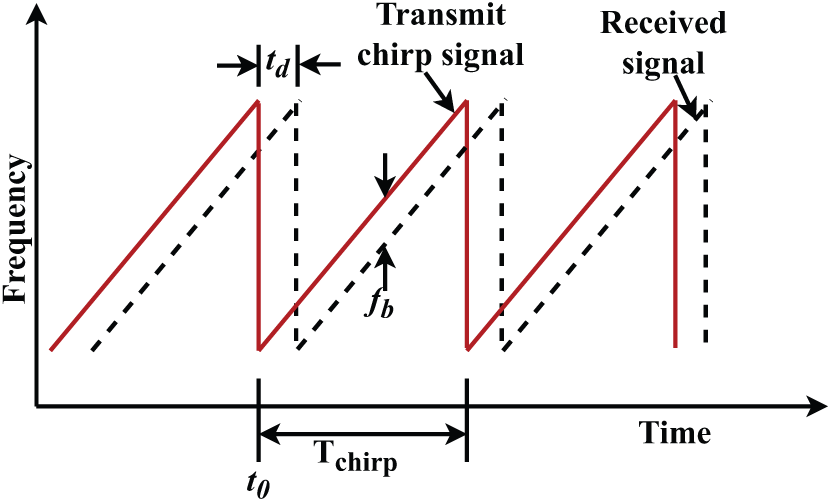
Figure 7: Fast chirp ramp sequence
OFDM [27] is a digitally modulated waveform comprising a set of orthogonal complex subcarriers. In vehicular radar applications, modulation symbols are mapped onto the complex amplitudes of these subcarriers. The orthogonality among subcarriers is ensured by designing each subcarrier to complete an integer number of cycles within the duration of an OFDM symbol, also referred to as the evaluation interval. To mitigate inter-carrier interference (ICI), the subcarrier spacing must exceed the maximum expected Doppler shift.
At the receiver, the radar modulation symbols can be efficiently demodulated using the FFT, making OFDM a suitable choice for digital vehicular radar systems. The range profile is extracted through frequency-domain channel estimation. Range and velocity estimations are performed along two distinct dimensions. Specifically, target velocity estimation can be viewed as a decomposition of the conventional two-dimensional matched filtering process into two one-dimensional matched filters, each is applied independently in its respective measurement domain.
2.4.6 Phase Modulated Continuous Wave
The PMCW waveform [28] consists of a sequence of periodically transmitted symbols that phase modulate a carrier frequency. The estimation of the target range is performed through the correlation between the received and transmitted signals. PMCW radar systems require sampling across the full bandwidth of the transmitted signal, necessitating high-speed sampling and high-resolution analog-to-digital converters (ADCs). Binary PMCW waveforms are commonly employed for automotive applications due to their simplicity and robustness. Binary PMCW is usually used for automotive applications. A PMCW waveform consists of a few symbols of binary nature
where
where
2.4.7 Combined Frequency Shift Keying (FSK) Modulated Waveform and FMCW Waveform
This waveform helps to remove ghost targets and accurately detect multiple targets with high-range resolution for short ranges. Here two-stepped Linear Frequency Modulated Continuous Waveforms (LFMCW), (designated as X and Y) are used, having the same sweep bandwidth and center frequencies, but split by a specific frequency,
Orthogonal waveform using TDM: In TDM MIMO automotive Radar, one transmitting antenna transmits a signal at each time slot. A specific antenna transmits N chirps at each time slot with a switching delay of
Orthogonal waveform using FDM: In this method, different carrier frequencies modulate the transmitter signals, and then these are separated from each other in a way that the nth FMCW chirp is shifted by frequency
Orthogonal waveform using DDM: In this technique, a total N chirps are transmitted in a sequence with
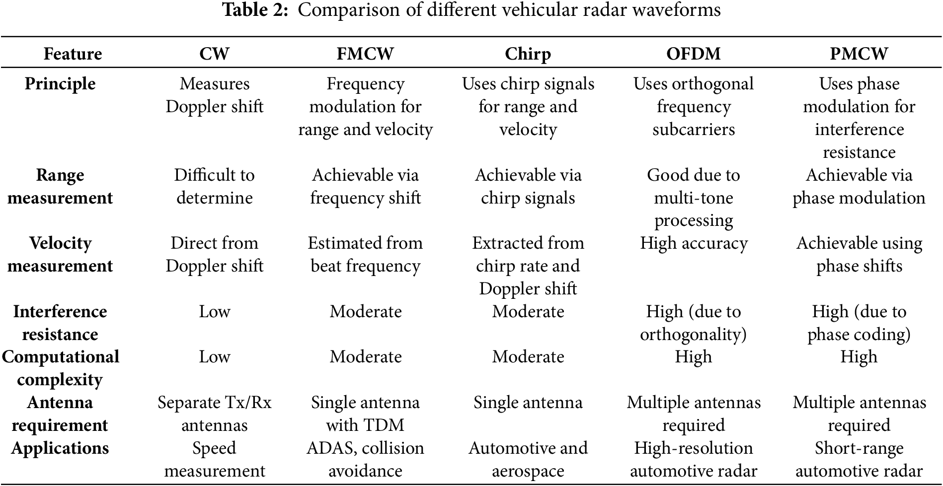
Table 3 presents an analysis of the different types of waveforms, generally used for automotive Radar, based on range and Doppler resolution values.
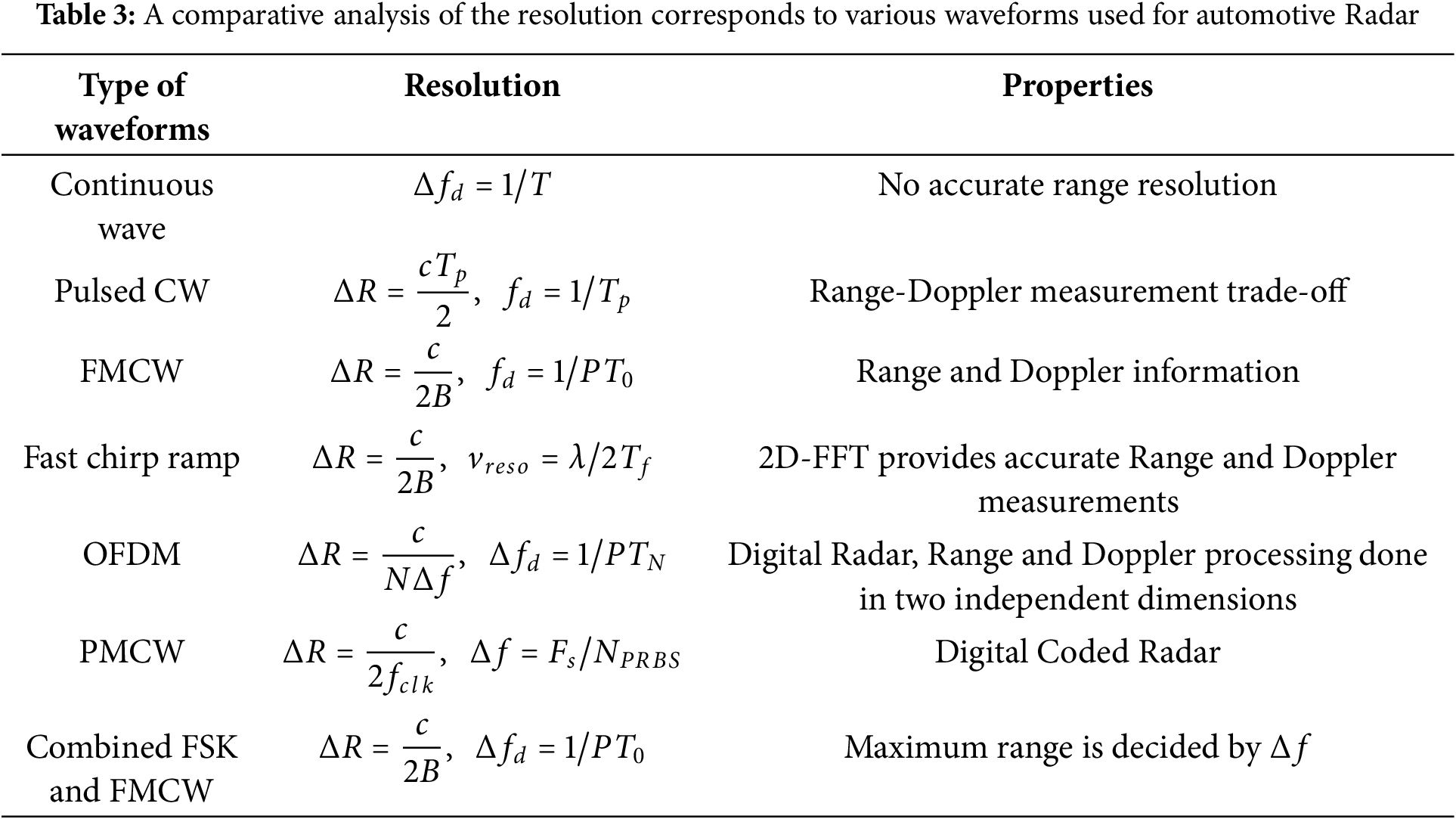
B = Radar bandwidth, T = time duration when data is obtained, N = samples used in CW and carriers used in OFDM,
For automotive Radar, conventionally, the FMCW chirp waveform is used due to the advantage of 2D-FFT processing for accurate range and velocity estimation. An RF sweep bandwidth increases the range resolution, and a fast ramp slope helps to achieve maximum unambiguous relative velocity. The fast ramp slope and wide IF bandwidth facilitate the separation of targets in the beat frequency domain, ensuring that the noise from a strong target produces less interference during the detection of a weak target. Recently, however, PMCW Radar has been preferred for automotive applications due to its capability to separate weak RCS targets from those of strong RCS targets. Binary PMCW Radars also provide no range-Doppler coupling and integration of Radar and communication waveforms. Polyphase-coded spread spectrum Radar system can be used for estimation of RCS over ultra-high-frequency radio channels [1,16,33–35].
2.5 Waveform Interference in Automotive Radar Systems
Interference due to Radars occurs when multiple Radars are in proximity, and the interference level depends on the in-between distance and the waveform pattern [36]. A particular vehicle fitted with an interfering Radar present at a distance R, is considered to create interference for a victim Radar. Here, the interfering radar acts as a target for the radar, which is assumed to be a victim. The interference-to-noise ratio (INR) measures the sensitivity of a victim Radar to interference. It depends on the variables of the interfering Radar and the victim Radar, the interfering Radar’s signal modulation pattern, and the demodulation process of the victim Radar. The interfering Radar is considered to have a bandwidth B, and at the victim, Radar, the power spectral density (PSD) of the interference is written as [6],
where
where
When the victim FMCW signal overlaps with the interfering FMCW signal, this results in a specific type of interference. After down-conversion at the radar receiver, the interference appears as a linear chirp signal that sweeps across the radar’s passband, occupying a wide bandwidth. After bandpass filtering, the interference signal becomes an “impulse-like signal” in the time domain. The slope and relative timing of the frequency modulation of both the victim and interfering radars determine the position and width of this interference signal. The difference in frequency modulation (FM) sweep rates between the interfering radar and the victim radar, along with their timing and frequency alignments, determines the bandwidth of the interference observed after down-conversion in the victim radar. Type A: interfering Radar and Radar assumed to be the victim, sweep with similar time duration
Type B: interfering Radar and victim Radar sweeps with similar time duration
where
This kind of interference is noticed when the “interfering PMCW” signal overlaps the victim PMCW signal. A PMCW interference is assumed with arbitrary, noise-type biphase coding with chirp rate
In both cases of FMCW victim and PMCW interferer or PMCW victim and FMCW interferer, the interference appears like noise in time and frequency domains. The INR is the same.
The techniques for interference mitigation in automotive Radar can be classified into two categories: techniques at the transmitter (such as frequency hopping and timing jitter) and methods at the receiver (such as time domain excision). Transmission techniques are usually designed to ensure that separate Radars transmit in a way where the signals are nearly perpendicular to each other in domains like time, frequency, or polarization. Mostly, interference mitigation is done at the receiver side. For FMCW-FMCW interference, a matched filtering is usually adopted to obtain integration gain for a constant frequency signal considered as a target and the interference spreads as noise [6]. For PMCW on PMCW interference, Code Division Multiple Access (CDMA) ensures that every Radar has a unique spreading code, and the interference becomes a wide-band noise signal. An FMCW interference is similar to a jammer in a spread-spectrum system for a PMCW victim Radar, and adaptive filtering can be used for mitigation. A PMCW interference on an FMCW victim can be reduced by separation in the polarization or frequency domain. Additionally, Neural network (NN) methods can be used for mitigating multi-channel interference [37]. The signal separation neural network can separate the interference from the beat signal, making it interference-free, and reconstruct the signal.
3 Target Detection and DOA Estimation
3.1 Signal Processing for Target Detection
A signal processing framework [17] is required for target detection with automotive Radar. An automotive Radar is considered to transmit a series of identical waveforms (like FMCW chirps, PMCW symbols, or OFDM). These transmitted waveforms are reflected from the targets and clutter and received at the receiver end, where they are down-converted as a combination of various Radar signal echoes along with additional noise from the receiver. The work aims to reduce additive noise and detect and then classify echoes obtained from various objects that are separable in the spectral domains of Doppler, range, and Direction of Arrival (DOA). For i =
where
where
where
where
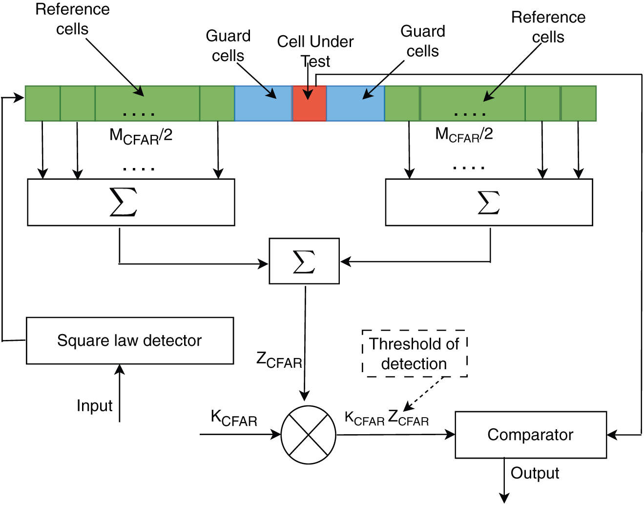
Figure 8: Working principle of the CA-CFAR method
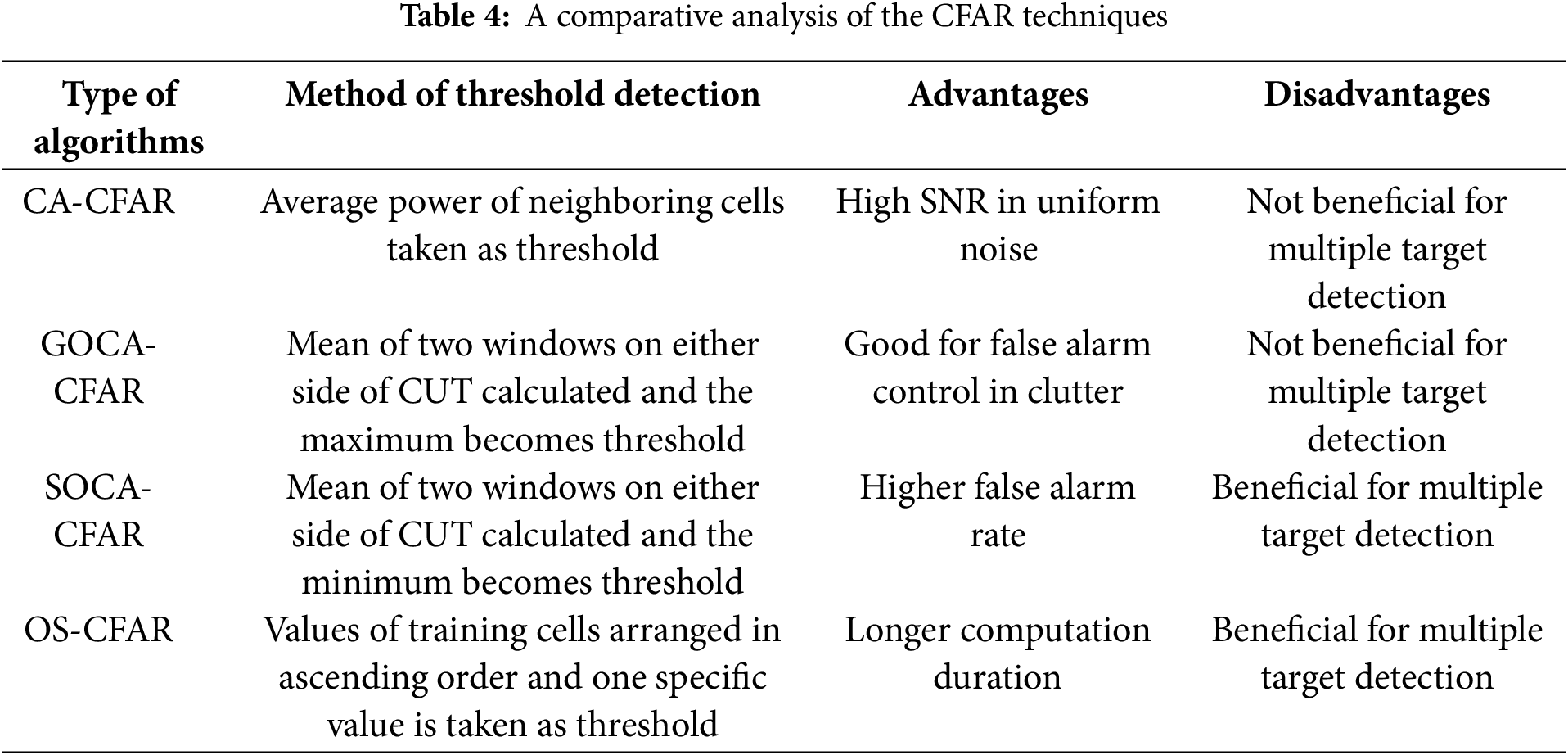
In Greatest-of-cell-averaging (GOCA-CFAR), two windows are considered on either side of the CUT, each having the same number of training/neighbouring cells. The mean of these two windows is calculated, and the maximum value of these mean values is taken as the threshold value. On the other hand, in Smallest-of-cell-averaging (SOCA-CFAR), the mean of the two windows is calculated, and the minimum value of these is taken as the threshold. In Order static CFAR (OS-CFAR), the values of the training cells are organised in ascending order, and one value is selected. This OS-CFAR detector is used in [39] for targets in micro-motion, and to cluster these targets, the image dilation algorithm is applied. Inclusion of deep learning techniques such as Convolutional Neural Network (CNN) [40] provides an increased rate of detection of targets compared to CFAR. A comparative analysis of these CFAR methods is presented in Table 4.
Clustering and tracking methods are adopted for additional detection required for automotive radar. Tracking of the target mainly includes prediction, association, and update procedures, as observed in the case of the Kalman filter. Tracking helps to improve target localization, deduce accurate velocity and trajectory, and create a picture of the target’s surroundings. The final task is called classification, where knowledge of the detected and then tracked target is obtained from echoes received from the target. This is achieved using selected micro-Doppler features, spatial spread, and other parameters.
3.2 Direction of Arrival (DOA) Estimation
Under real-world road conditions, an unknown number of signal echoes from targets in various directions may arrive at the receiver antenna. These target echoes, combined with noise and interference, pose significant challenges for reliable target detection and tracking. To enable accurate beamforming and to place nulls in the direction of interfering signals, precise estimation of the DOA of the desired target signal is essential. Various DOA estimation techniques for target echoes are illustrated in Fig. 9.
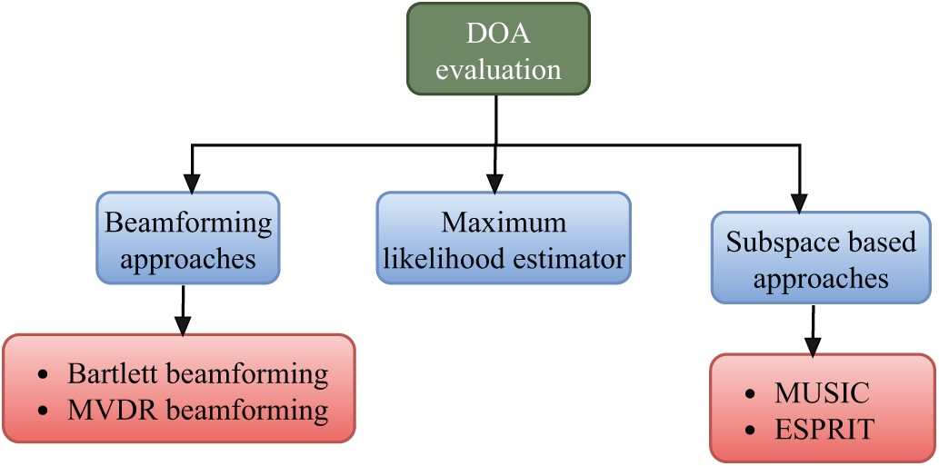
Figure 9: DOA evaluation techniques
A radar signal model is presented in Fig. 10 to estimate the DOA of the received signal.
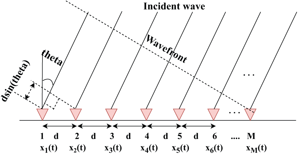
Figure 10: Signal model for DOA estimation
An automotive radar system is considered to contain a series of M antenna elements on which signals from
where
where
With H denoting the Hermitian response. Then the power at the output of the array of sensors is given as,
where E[.] is the expectation operation and
Beamforming is a technique used to create a desired radiation pattern by coherently combining signals from multiple antennas, each weighted according to its appropriate value. This process enhances signals arriving from a specific direction while suppressing interference and noise from undesired directions. The Bartlett algorithm, also known as conventional beamforming, is used to enhance the signal from a specific direction by compensating for the phase shifts of the incoming wavefront. The optimal weight vector in the Bartlett method ca be written as,
The limitations of Bartlett beamforming include: i) Applicable only for a single source of signal, ii) In the presence of multiple sources, it provides low resolution, resulting in ambiguity.
3.2.2 Minimum Variance Distortionless Response (MVDR)
In this algorithm, a persistent gain is maintained for the signal from a desired direction, and a lesser weight is added to the direction of the interfering signal and noise. The weight vector is given as
The weight vector for beamforming angle
The power spectrum at angle
This method provides improved resolution than Bartlett, but not as much as subspace methods. To enhance the angular resolution of beamforming algorithms, a method can be employed to determine the transformation vector that represents the relationship between received signals and create extrapolated elements outside the region of the array’s actual antenna elements [42]. With both original and extrapolated signals, the direction of the target echo is estimated with higher resolution.
3.2.3 Multiple Signal Classification (MUSIC)
This method is based on the subspace approach, where the covariance matrix is decomposed into a signal subspace and a noise subspace. The steering vectors are observed to be orthogonal to the noise. In the spatial power spectrum, a peak provides the required direction. Considering the equation of the received signal as shown in (29) and (30), the covariance matrix is presented as,
where
where the eigenvalues are sorted as,
The parameters can be defined as,
The basic principle of the MUSIC algorithm is that for a real source direction
Therefore,
The MUSIC algorithm observes the angles
The main disadvantages of the MUSIC algorithm are that it requires prior knowledge of the signal sources and its complex computation.
The MUSIC algorithm can be summarised as follows:
1. The sample covariance matrix is computed, using the source covariance matrix
2. The Eigenvalue decomposition of
3. The noise subspace
4. For each angle
5. The DoAs are obtained from the peaks of the pseudo-spectrum.
3.2.4 Estimation of Signal Parameters via Rotational Invariance Techniques (ESPRIT)
This method, ESPRIT, is computationally less complicated than MUSIC as it does not consider all direction vectors. The subspace of incident signals is lengthened by two responses displaced by a recognized vector, using which the DOA can be obtained. The equation of the received signal is presented in (29) and (30). The assumptions for the ESPRIT algorithm can be stated as,
• The array needs to have a structure of translational invariance (e.g., two identical subarrays).
• Prior information is present for the number of sources
• The source signals are considered uncorrelated.
• Likewise, the noise is uncorrelated with the signals and spatially white.
Now two overlapping subarrays of size
where
Hence, the subarray outputs can be written as:
Here,
For the estimation of Subspace, the equation form the data matrix:
The sample covariance matrix is computed as follows:
The eigen-decomposition of
The matrix
For the estimation of Rotational Invariance and Eigenvalue,
It is assumed that,
for an unknown matrix
For the estimation of
Then the he eigenvalues of
Every eigenvalue needs to satisfy the following condition:
Finally, the angle of arrival can be estimated by using:
The ESPRIT algorithm can be summarised as follows:
1.
2. The covariance matrix
3. The signal subspace
4.
5. Estimation of
6. The eigenvalues
7. Finally, estimation of the DoAs is done:
Here, the eigenvalues of
A MUSIC algorithm with enhanced beamspace can lessen the computational complexity and storage space, which is beneficial for automotive Radar [45]. The parameter space can be reduced by utilizing prior information to improve beamformer design. To mitigate the consequences of a lower SNR value and incorrect sample covariance in a single snapshot, a modified estimator can be employed, which considers the relationship between a signal with an interference model of sample covariance and the subspace model. Furthermore, to enhance direction estimation for two closely spaced targets, the averaging of sub-matrices of sample covariance evaluation and the utilization of the Toeplitz structure are employed. This new algorithm offers a higher resolution probability than conventional MUSIC at the same signal-to-noise ratio (SNR). For the processing of range and angle, a single-snapshot MUSIC is used in [46], which reduces the computational complexity. Another process involves obtaining DOA with single-snapshot MUSIC and evaluation of the performance with analog-to-digital allocations [47]. A new way for better resolution of angles is the application of a two-stage MUSIC algorithm [48]. Here, a crude estimation is initially performed using MUSIC. However, this estimation won’t be accurate if the targets are closely placed and have low SNR. Based on these values, each antenna element is directed to specific directions using a calibration technique that focuses on signals coming from particular directions, as presented in the first stage. The Root Mean Squared Error (RMSE) values of this new method with Root-MUSIC are less than those of standard Root-MUSIC in the low SNR region. In [49], a compressive sensing alternating descent conditional gradient (CS-ADCG) algorithm has been used. Using a gridless process and minimization of the atomic norm, the observation scene has been discretized to prepare an atomic set. The signal sources’ angles are obtained by measuring the inner product of this atomic set with fragments from every iteration and are used as primary values for searching. Finally, a function for mapping is made of the sources of the signal, and gradient descent is applied for iterative optimization. This step is conducted in a continuous domain to reduce the off-grid effect. To determine DOA in the presence of interference, the variational mode decomposition method is used. Then, with the signal-to-interference ratio obtained from this algorithm, a weighted MUSIC algorithm is applied for obtaining DOA [50].
The time complexity of MUSIC or MVDR is obtained as
A different method of lowering the computational complexity is by application of digital beam-forming (DBF), which is suitable for dynamic environments as seen in road scenarios of automotive Radar [58]. A 77 GHz automotive Radar uses an improved angular resolution DOA algorithm, which is formed by a bigger virtual array using the relative motion observed between the automotive Radar and targets. The proposed DBF-based method can obtain a crude evaluation of the target angle. The radial velocity produced by the relative motion observed between the radar and targets is taken as if only produced by radar, with the targets motionless. Thus, alongside the vehicle’s moving direction, a velocity that differs from its actual velocity can be measured. Lastly, the positions of the array for
Sparse matrix-based representation of Radar signals can be used for DOA estimation in MIMO Radar [60]. For sparse uniform linear array (ULA) structure, FMCW radar is preferred as it can provide highly accurate range information even in high SNR situations [61]. A sparse matrix depiction is developed for a bistatic model of Radar for 2D-location, i.e., range, DOA, and Doppler estimation [62]. Here, the road is characterized by a Cartesian map using which the targets’ coordinates and total multi-path Doppler for target velocity are estimated. In a sparse version of the raw Radar data, after controlling the bistatic formation’s geometry, the source vectors have a familiar support set, which helps in the application of group-sparsity (GS) based optimization. This algorithm for estimating 2D location and Doppler performs better compared to MUSIC. A further addition to this algorithm is the application of a 3-dimensional (3D) multi-static FMCW signal model, followed by an evaluation of the multi-target location and Doppler method using the GS methodology [63]. Furthermore, an association of multi-target parameters via cross-correlation and an ESPRIT algorithm, as well as based on Least Squares, is demonstrated. The GS joint shows better results than MUSIC at every level of SNR in the evaluation of Doppler and location. Additionally, the GS method can be used to determine the Doppler frequency first, and then the Doppler parameters are used for obtaining range parameters, and finally, the DOA is evaluated with these target parameters [64]. A signal processing method for DOA measurement based on Compressive Sensing (CS) theory is presented, which provides good resolution and accuracy while allowing an improved degree of design [65]. This algorithm enables the utilization of configurations with sparse antennas, featuring a reduced number of transmitter and receiver channels, while maintaining a larger effective antenna aperture. The authors have provided four sparse reconstruction algorithms along with the MUSIC algorithm. Orthogonal Matching Pursuit (OMP) is better suited for automotive Radar applications, as it offers improved detection efficiency and is faster than MUSIC. A method for ghost target detection is shown in [66] where the CS method is used for angle estimation of direct paths and multipaths.
Deterministic maximum likelihood (DML) is a parametric-based DOA estimation approach that estimates DOA by a projection of vectors of the received signal to the steering matrix’s null space. In [67], different transmit signals having orthogonal properties are generated with space-time block codes, and depending on the number of transmit antennas, the transmit signals have their phases shifted at orderly intervals. Each of the signals transmitted is matched to its respective transmitting antenna by applying the DML algorithm to find the proper array for DOA estimation. Upon identifying the signal transmitted from the initial transmitter antenna, the highest velocity to be detected is not compromised, and the accuracy of DOA analysis is improved. When the transmitted signals are not matched, the correlation value of the received echo signal and the steering matrix is degraded, and DOA estimation is worsened, even if the number of targets is appropriately detected. Based on ML assessment [68,69] MARS-a super-resolution real-time DOA used for automotive Radar. Here, the evaluation results from earlier timestamps are used to create an adequate and reduced search space. To decrease computation time, problems at every step are decomposed into separate sub-problems, and the GPU is utilized for parallel computing. Through simulation-type experiments, it has been demonstrated that only MARS can handle up to one hundred bins consisting of reflection points with a resolution of 1∘ within 1 ms. A DOA estimation based on Fast Variational Bayesian method helps to lessen the high sidelobes in sparse arrays and improve resolution for closely placed reflectors [70]. The implementation of sparse Bayesian algorithms for DOA evaluation, which provides improved accuracy and lower hardware costs, is demonstrated in [71].
Machine learning algorithms for DOA measurement can be classified based on Regression, model order methods, and spectrum [72]. To improve DOA estimation and reduce computational complexity, in [73], the authors utilize a look-up table (LUT) based on data storage, which can mitigate measurement errors. Then, the authors propose Support Vector Machine (SVM), an ML classifier, to decrease the high storage complexity. The ideal azimuth selection issue is considered a multi-classification problem, in which a considerable quantity of training samples is obtained from the ultra-SRR and used to improve the classifier. Depending on these data for training, the SVM algorithm is applied to receive more precise azimuth information in SRR. Table 6 contains a detailed analysis of research works available regarding DOA estimation of targets using automotive Radar.
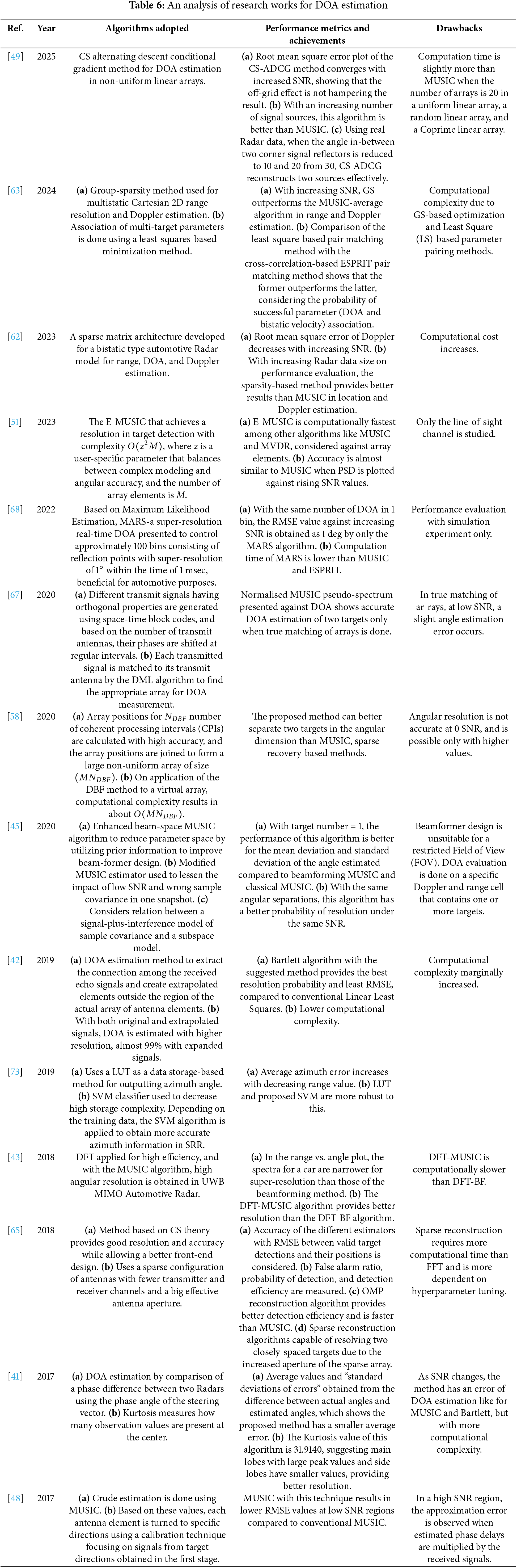
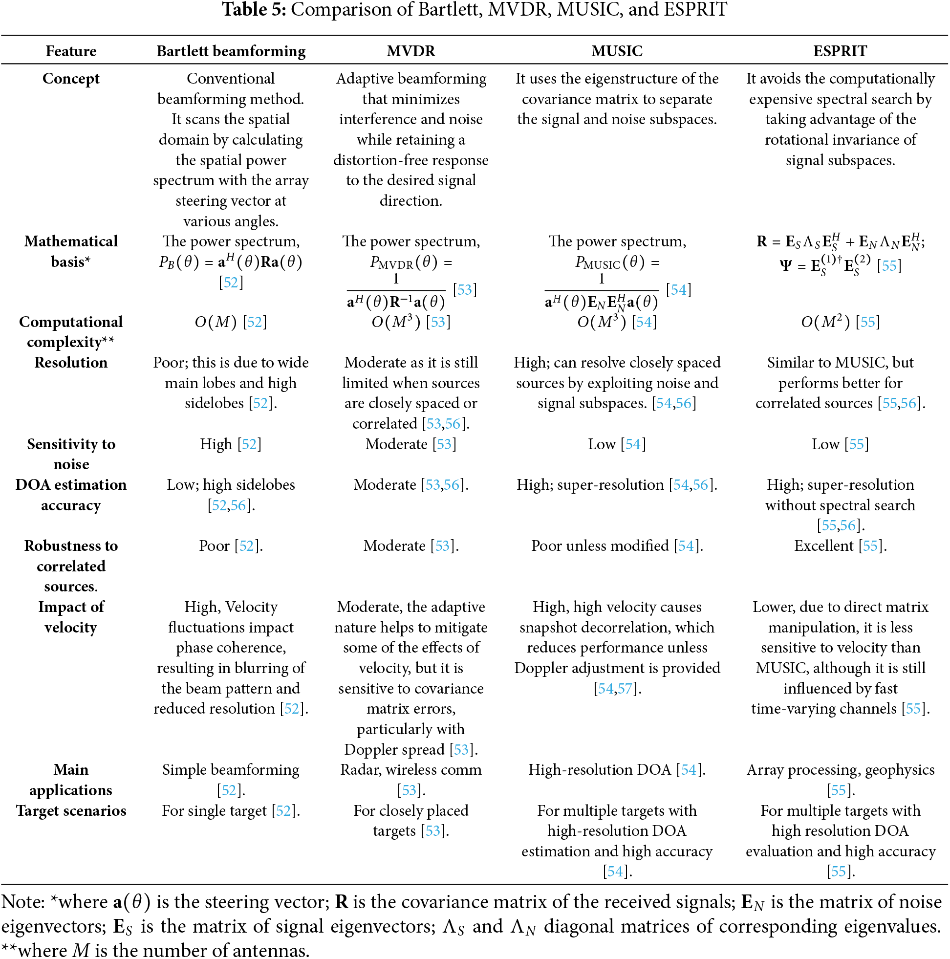
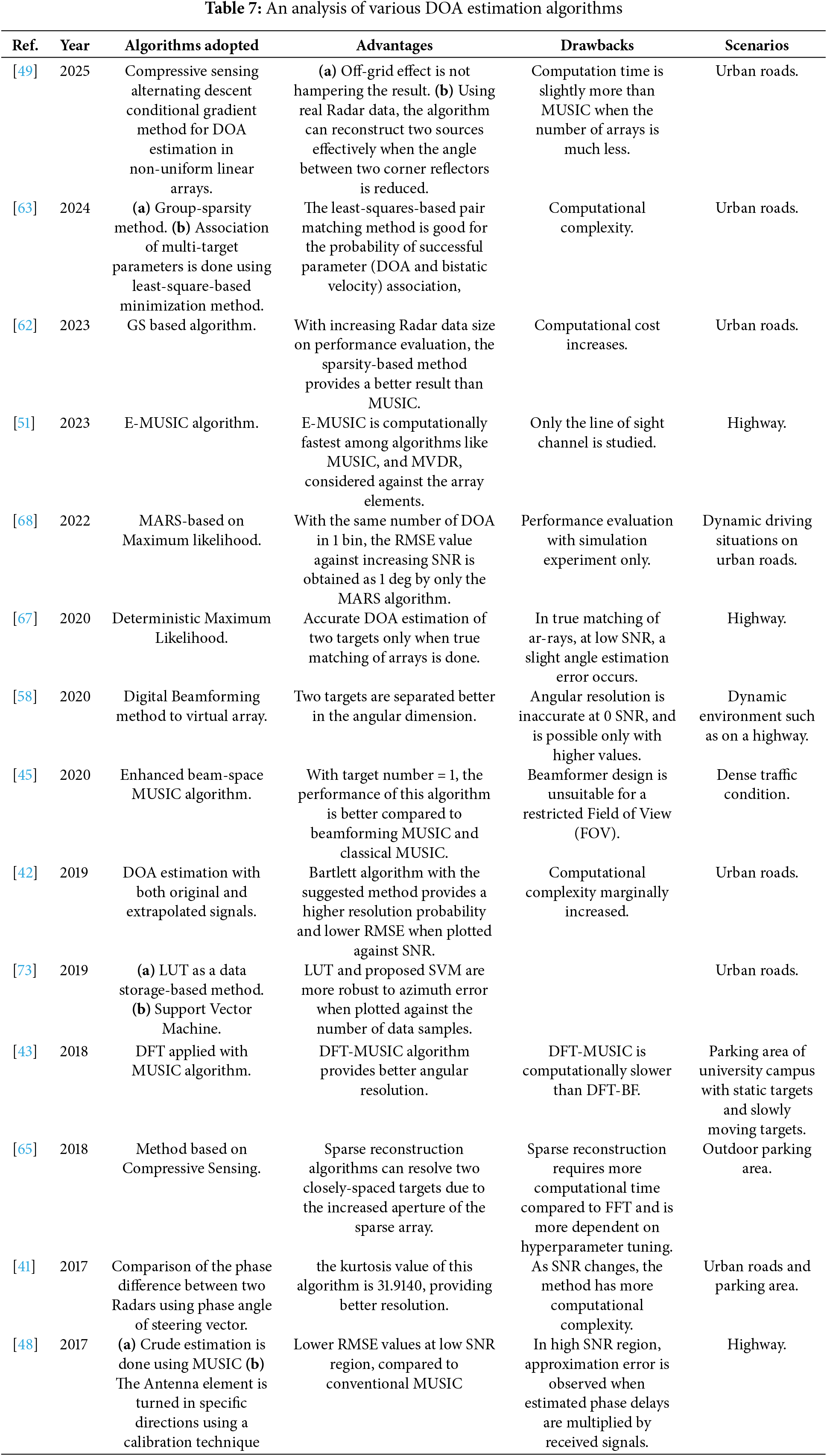
Table 7 contains an analysis of various DOA estimation algorithms.
After target detection by Radar, filtering and tracking techniques for obtaining target motion dynamics are required to stay informed about the target’s position and avoid collision [74,75] as in the ACC application. Different target modeling models are present, like dynamic target modeling and static target modeling, which are further categorized into occupancy grip mapping, amplitude grid mapping, and free space mapping [76]. Fig. 11 draws a flowchart of the target tracking signal processing method.
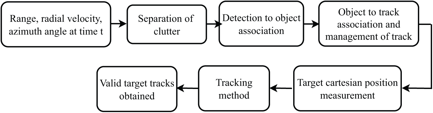
Figure 11: Signal processing for target tracking
The target parameters measured are range, velocity, and azimuth angle obtained at time instant t. The target is separated from clutter by discriminating between moving and stationary targets, where stationary targets are not considered. Object association is achieved by grouping multiple detections from the same target into a single object. When an object does not match any existing track, a new track is initiated, resulting in valid and false tracks. Only valid tracks of real targets are input to the tracking filter. The target position represented in Cartesian coordinates obtained from range and angle measurements is fed to tracking filters. The output from the tracking filter is a valid track for a particular target.
The main characteristics of multi-target tracking are [77,78]:
1. Motion model for the target.
2. Prediction and update of the target state.
3. Data association of measurements of tracks.
4. Target Track Management applied for track initiation, confirmation of track, and termination of track.
To detect a target vehicle, motion models are utilized, where the parameters of the target are assembled from sensor data. These models are designed according to the movement of vehicles and classified as constant velocity (CV), constant acceleration (CA), constant turn rate (CTR), and constant turn rate and acceleration (CTRA).
4.2 Prediction and Update of Target State
Track initiation establishes a sufficiently accurate track in terms of position, velocity, and direction within the shortest time possible. The Kalman filter (KF) is typically used to estimate the location of actual targets at the current instant in time, utilizing prediction and update processes. The Bayesian method is also being introduced for this purpose.
The KF is a recursive filter used to estimate the state of a discrete-time linear type dynamic system from noise-filled measurements. It consists of a Prediction step and an Update step. Prediction step: A new value called the predicted value is assumed based on the initial value, and then the error present in the prediction is obtained according to various noises in the Radar system. Predicted value,
where F is the state transition matrix,
where Q is noise and T stands for transpose. Update step: The actual measurement coming from the Radar is obtained and named as the measured value. The difference between the measured and predicted values is evaluated, and then it is decided which value to keep based on the Kalman gain. Based on the Kalman gain, these new values and new errors are calculated, which will be the predictions done by the KF in the first iteration. The Kalman gain is the parameter that determines the weight assigned to predicted and measured values. It determines whether the actual value is closer to the expected value or the measured value. The output of this Update step is fed back to the predicted state, and this cycle continues until the error between predicted and real values conve rges to zero.
where H is state transition matrix containing no unwanted information,
where
These new
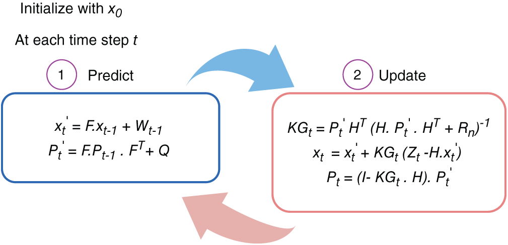
Figure 12: Kalman filter algorithm
4.2.2 Extended Kalman Filter (EKF)
The limitation of the “Kalman filter” is that it works with a Gaussian distribution and linear functions. Radar data involves non-linear functions, which must be approximated to make them linear. This approximation is typically performed using the Taylor series, and the EKF can be applied afterward. Prediction step: The prediction step is similar to the Kalman filter.
where F is a matrix of state transition,
where Q is noise and T stands for transpose. Update step: the difference in-between the measured value and the actual value is given as,
where
where
Fig. 13 shows a pictorial presentation of the Extended Kalman filter method.
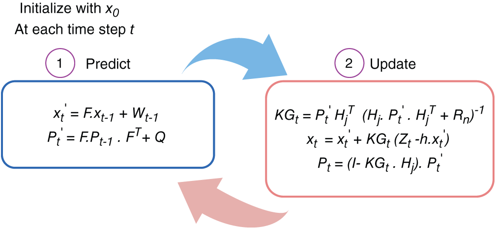
Figure 13: Extended Kalman filter algorithm
4.2.3 Unscented Kalman Filter (UKF)
The UKF is similar to the EKF and tries to address its problems. Here, the transformation is a nonlinear unscented transformation and is considered a replacement for the linearization process in EKF. In this method, a precise nonlinear function is employed to approximate the probability distribution of the state.
To work with non-Gaussian Radar systems, Bayesian filtering and the particle filter (PF) are sometimes employed. With the help of random samples, this method estimates the state Probability Density Function (PDF). The model for the system can be shown as,
where F is a transition matrix and
where H is taken as the transition function and W is taken as zero-mean white noise. The PF algorithm can approximate the posterior PDF P(x(t)|Z(1:t)) by particles, which are a set of weighted random samples. The first prior distribution of the state P(x(0)) and PDF P(x(t−1)| Z(1: t−1)) at time (t−1) are assumed to be known. The PDF is written as,
The prediction is then updated with the help of the current measurement y(t) based on Bayes’ theorem,
in which, P(y(Z)|Z(1:t−1)) is a normalizing constant. The optimal state can be derived as
A limitation of this method is that the unknown integrals are hard to compute, so approximations are needed.
A single target localization method by applying a collocated MIMO-monopulse approach to FFT processing is adopted in a real-life experiment [79]. To improve the velocity uncertainty of a moving target, a cascaded KF as described in [80], can be applied, where KF is first applied on polar coordinates to derive velocity and predict the acceleration. Next, an EKF is used to improve velocity measurements and minimize measurement error when the motion state is in Cartesian coordinates, and measurements are provided in polar coordinates. An improved adaptive EKF is used in [81] to enhance the robustness and accuracy of the tracking process. A cubature Kalman filter (CKF) applies the cubature rules to approximate recursive Bayesian estimation integrals with a Gaussian assumption. The square-root CKF (SRCKF) algorithm distributes the factors, which are the square roots of the predicted and posterior error covariance matrices, to prevent the square rooting of the matrix. The iterative SRCKF algorithm in [82], iteratively optimizes the SRCKF measurement and update processes by the Gauss-Newton method, leading to a lower error component. In [83], a threshold method is first used to filter out ghost targets and empty targets. This is followed by application of the Adaptive Interactive Multiple Model Kalman Filter and the Hungarian algorithm for association and tracking of multiple targets, which reduces the error as compared to conventional UKF algorithms. In [84], a multi-target tracking algorithm based on a 4D Radar point cloud has been proposed for obtaining the intensity, location, velocity, and structure of the targets. The method provides compensation for point cloud clustering, velocity, static state, and dynamic state updates, as well as 3D border generation of the dynamic target using the Kalman filter, contour updates of the static target, and a target trajectory control procedure. Tracking of targets in the presence of velocity ambiguity requires a tracking algorithm with TDM where disambiguation of Doppler is done before angle estimation [85].
A reweighted robust PF (RR-PF) is proven to improve state values in a nonlinear model and is more robust to outliers [86]. The method utilizes inputs from the particle weights of true particles and filters out inputs from unreliable particles through the discriminative treatment of detected Radar data. A track-before-detect (TBD) algorithm uses the targets’ kinematic constraints on road and graph theory algorithms to define every plot as a potential target or clutter [87]. The algorithm involves a discriminant metric, which refers to mathematical calculation rules of a plot and its trajectory, followed by the state transition of the plot, and requires transition conditions. The post-processing is done for motion state estimation of confirmed targets, after which significant results in target detection and effective clutter removal are observed. A multi-frame TBD can adjust the threshold value of detection depending on the existence of mobile targets present within the Radar field-of-view and also considers the self-positioning errors of the ego vehicle [88]. Another application of TBD is the motion compensation technique on the dynamic programming-based TBD [89], which works for ground Radars to decrease the error of the conventional algorithm. In [90], the Cramer-Rao lower bound method is applied to detect the location and velocity of a mobile target, and an active sensing application is further used to improve tracking accuracy.
Linear Regression with KF: A machine learning algorithm like Linear regression can be applied with KF for more accurate estimation of target parameters. Linear regression helps identify a statistical relationship between an independent variable and a dependent variable. Here, time (t) can be assumed as independent and ‘
The motion in both ‘
4.3 Data Association and Measurement of Tracks
Data association is used to combine multiple detections from the same target into a single object. If an object does not match the current track, a new track has to be initialized. Thus, valid and false tracks are produced. The valid tracks are considered for updating the states [91]. In the global nearest neighbor (GNN) algorithm, the association depends on the minimum Euclidean distances between measured and predicted values. However, this algorithm performs poorly in high-clutter regions.
The Joint Probabilistic Data Association Filter (JPDAF) algorithm is more efficient for tracking targets, where the probability of
A micro-Doppler-based leg tracking framework for pedestrian detection to enable behavioral signs within one measurement cycle has been presented in [92]. A model is designed to estimate the spatial movement of the feet, segment the body in a vertical format, and extract the reflection points resulting from leg movement. An elevation-resolving antenna is used. Then, EKF is used for target tracking. After data association is completed with Joint Probabilistic Data Association (JPDA), the reflection points can be assigned to a particular leg. Then the location, kinematic data, and velocity of each foot can be filtered. In [93], an Interacting Multiple Model (IMM) algorithm with the JPDA algorithm is shown to achieve tracking of multiple maneuvering targets. Since the effect of this algorithm is less pronounced in the nonlinear case, UKF with Doppler measurement is applied to achieve better position and velocity accuracy. In [94], the spatial distribution of the measurement model produced by a target vehicle is presented using a variational Gaussian mixture (VGM) model. For mapping of the extended target tracking problem, the Probability Generating Functional formulation has been used.
An adaptive strong tracking extended KF (ASTEKF) helps to lessen the impact of state transitions and parameter changes on the measurement process and for better resilience to interferences [95]. The adaptive attenuation factor is updated whenever the time fading factor changes, helping to mitigate the divergence problem in a tracking process. This algorithm offers enhanced capacity to track abrupt changes in the target’s motion states. A number of clustering algorithms are used for identification, investigation, and tracking of targets [96]. The Density Based Spatial Clustering of Applications with Noise (DBSCAN) clustering algorithm can be applied to range-angle data to obtain the centroids of the cluster points, which then provides the target position [97]. An imaging method for a target moving at high speed utilizes the Doppler Range Processing (DRP) method to achieve velocity and range resolutions, thereby obtaining coherent integration gains through range-Doppler processing [98]. Initially, Doppler processing is performed using the FFT on slow-time samples. A velocity bin interpolation method, and lastly, processing of the range is done via FFT over Doppler migration lines. The complexity of computation of this algorithm is calculated as
A hybrid smooth variable structure filter (SVSF) is presented in [99] by combining generalized time-varying smoothing boundary layer (GVBL) and Tanh-SVSF to prevent parameter sensitivity and control the unwanted chattering matter. A non-linear generalized variable smoothing boundary layer (NGVBL) parameter is used to create a hybrid switching scheme that leads to an ideal Kalman filter (KF) in cases of low model uncertainty. For solving data association and clustering problems, a Deep Neural Network (DNN), called Radar Tracking Network or TrackNet, can be used, which applies point clouds of Radar data from several time stamps to get desired objects on the road and provide the information on tracking [100]. In this architecture, features are extracted independently for each cell and timestamp using a PointNet++- based method that incorporates long-distance point sampling and multi-scale grouping. This is followed by processes of convolution and max-pooling applied to smaller point clouds within each cell. For extended object tracking, a measurement modeling and estimation method, known as the data-region association process, partitions an object into several regions. A simple measurement distribution is performed over each area, and a complex method is applied to the target [101]. Also, a new gating method is used for data association.
For multiple targets, a management process is required to filter false alarms and efficiently track them under changing detectability scenarios [102]. Tracks can be classified into two categories: provisional and verified tracks. After each measurement round, the values are updated and verified in the first phase. The remaining measurements are tested for association with provisional tracks in the second phase. If these measurements do not correlate with known tracks, they initialize new provisional tracks. After further examination, these tracks become either confirmed or deleted. For this purpose, the M/N test can be applied, where a provisional track is confirmed if a minimum M number of detections is obtained for N scans of data. If K or fewer detections are obtained for N scans, the provisional track is rejected. A composite method can be formed by combining two or more M/N tests by a logical OR operation. This will provide more accurate results with little increase in computational difficulty. For target tracking, a medium access control (MAC) technique has been adapted so that automotive Radars can have a common channel and suggest the best MAC parameter for a particular vehicle and corresponding road traffic [103]. Table 8 contains a detailed analysis of research works available regarding target tracking using automotive Radar.
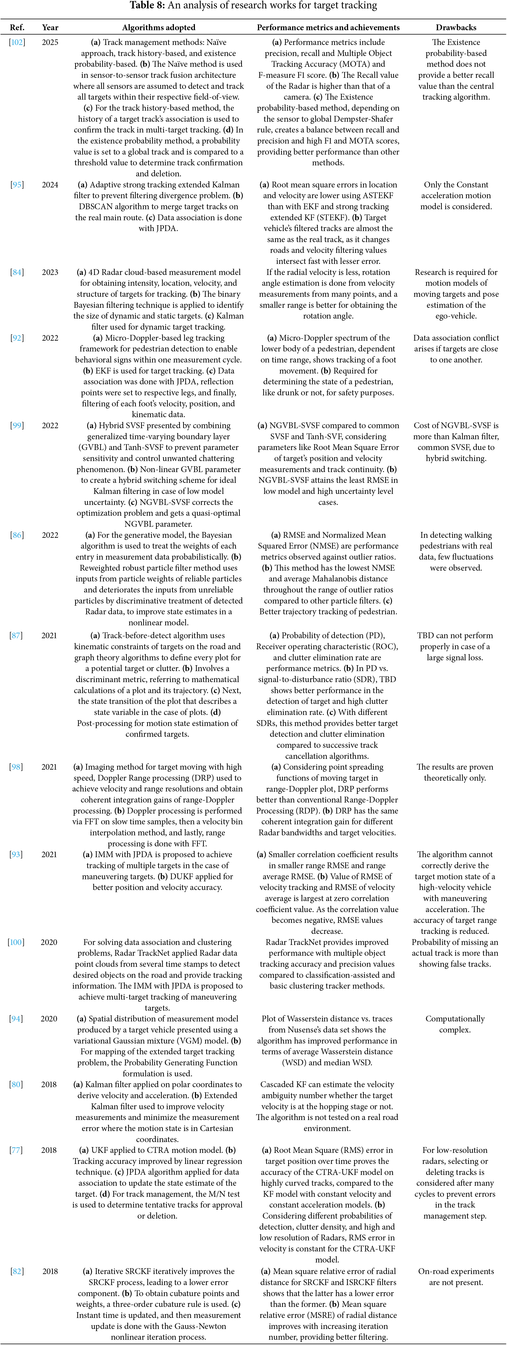
Table 9 contains an analysis of various algorithms for target tracking using automotive Radar.
5 Target Recognition and Classification
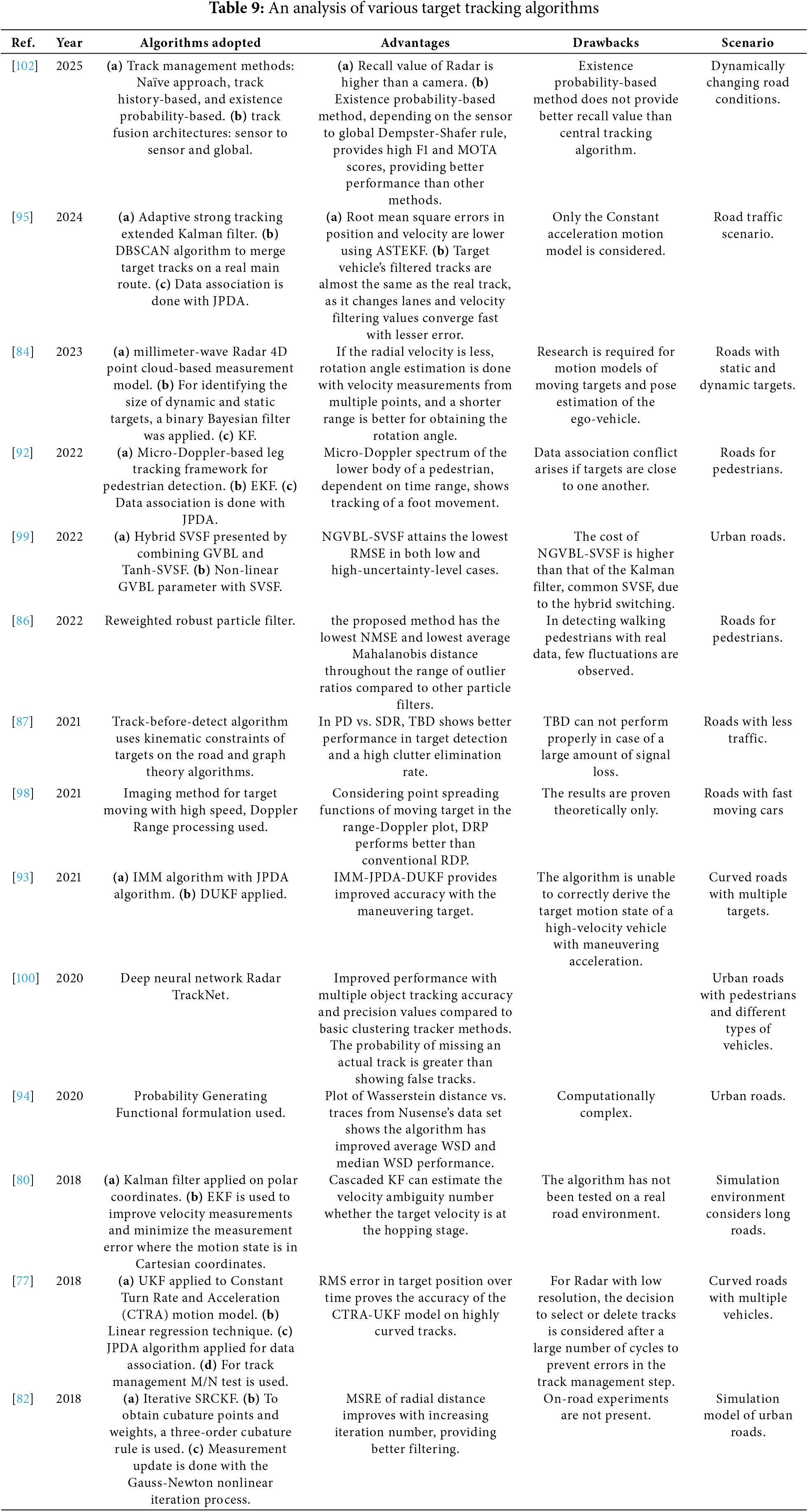
The road scenario in which automotive Radar operates is very cluttered, so the classification of targets with high accuracy is essential. A flowchart for the target recognition and classification process is depicted in Fig. 14. Using the raw Radar data, a potential target is observed and its features like RCS, range, and Doppler are extracted.
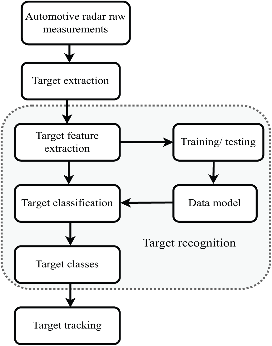
Figure 14: Signal flowchart of automotive radar for target recognition and classification
A training data set containing representative Radar data examples is required. Now, the data measured from the target is considered along with the training data. The result is classifying the new data, i.e., the new target, into different classes or categories. The target recognition problem in Radars can be addressed from an ML algorithm perspective. The principle of an ML is to find the direction from a group of unknown data and then utilize this to predict the next step in advance or classify the remaining data. ML algorithms are divided into three types: Supervised learning algorithms, Semi-supervised learning, and Unsupervised learning algorithms. The supervised methods are applied when training datasets are available to predict the output of the algorithm, and the well-known examples include K-Nearest Neighbor (KNN) algorithm, Support Vector Machine (SVM) algorithm, and Artificial Neural Networks (ANN). Semi-supervised methods are used when labeled data is insufficient and unlabeled data is used for training the algorithm; certain Convolutional Neural Networks (CNNs) fall into this category. Unsupervised algorithms such as K-means clustering and Principal Component Analysis (PCA) are applied when labeled data is not available for training purposes.
5.1 K-Nearest Neighbor (KNN) Algorithm
In the scenario of Automotive Radar data, the supervised learning algorithm, KNN algorithm [104], can be used to classify Radar signals into different categories based on their similarity to other signals. To derive this classifier, a training set containing representative examples of the Radar data is required. Data obtained from the Range-Doppler map is considered. The main steps for the KNN algorithm can be written as:
1. Calculation of distance between the fresh data point, known as query, and every data point in the training dataset with the help of a distance metric, e.g., Euclidean distance as used here:
where
2. This equation is conducted on each existing data point with the new data;
3. Once all distances are obtained, these are sorted in ascending order to find the k-nearest neighbors;
4. The k-nearest neighbors with the smallest distances are selected with
5. Lastly, the class of the query point is obtained based on the majority class among the k-nearest neighbors.
5.2 Support Vector Machine (SVM) Algorithm
The SVM is a set of supervised learning algorithms used to classify targets, regression, and outlier detection [23]. The SVM algorithm chooses the decision threshold from an indefinite quantity of probable ones, leaving the biggest margin between the nearest data point and the hyperplane, called support vectors. A classifier of linear type is of the form,
where
The issue of optimization is stated as,
This problem is expressed by defining the Lagrangian
where
After substituting
The initial problem of optimization can be finally given as,
So, if
A classifier based on bidirectional long short-term memory (LSTM) applies the feature of relative velocity, range, and signal amplitude to classify targets at ground level and targets at overhead on real roads, useful for collision avoidance [105]. FFT and cell-averaging CFAR (CA-CFAR) have been used for the implementation of this LSTM, which provides a precision of around
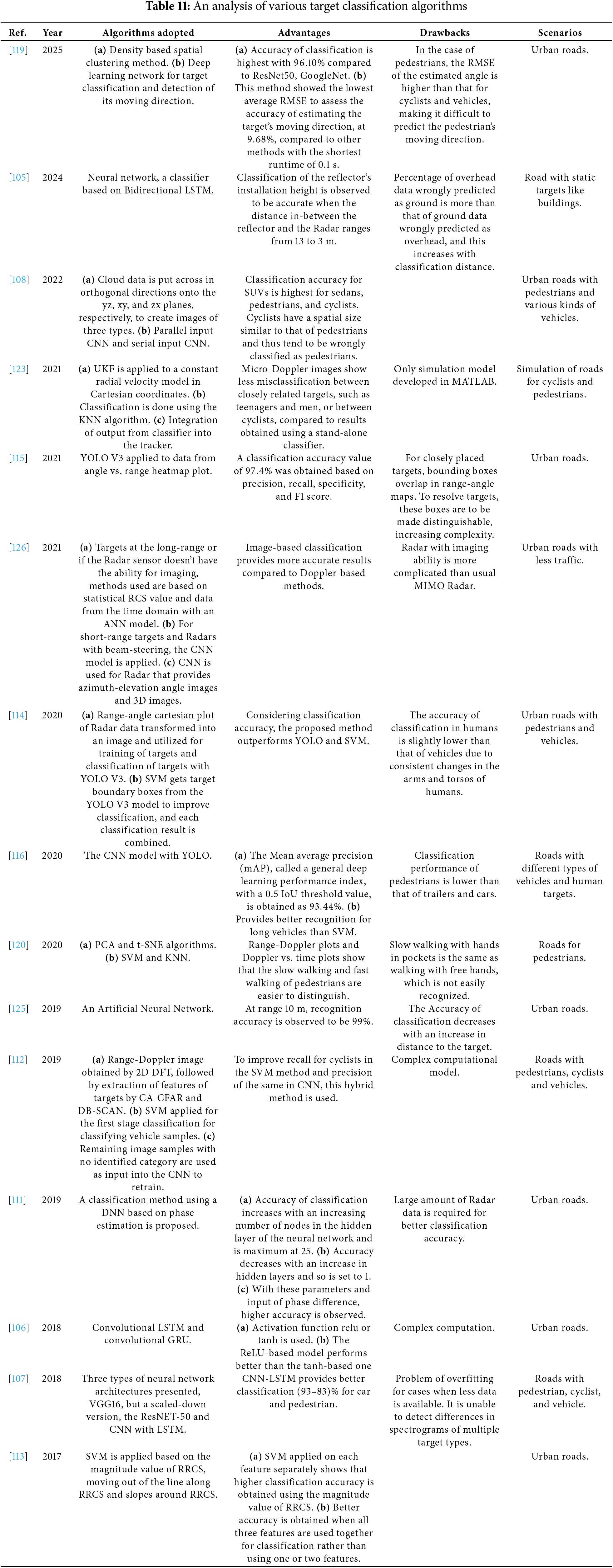
A hybrid method of SVM and CNN techniques for target classification is proposed in [112]. At first, the range-Doppler image is obtained by 2D DFT, followed by the extraction of features of targets by CA-CFAR and a DBSCAN algorithm. Then, SVM is applied for the first stage classification, and finally, the remaining image samples with no identified category are used as input into the CNN to retrain. Based on conventional RCS, Root Radar Cross Section (RRCS) is defined in [113], for real-time target classification using 77 GHz FMCW Radar. The RRCS is determined by using the amplitudes of the received and transmitted signals from the frequency domain. Hence, the reflection characteristics of targets can be extracted from the amplitude of the transmitted signal. The SVM can be applied to pedestrian and vehicle classification based on the proposed characteristics obtained from RRCS. Another method of using SVM in conjunction with a Deep Learning (DL) model, specifically You Only Look Once (YOLO), for classifying vehicles and humans is presented in [114]. The range-angle Cartesian plot is transformed into an image and used for training and classification with the YOLOv3 model. The SVM utilizes target boundary boxes from the YOLO V3 model to enhance classification, and by combining each result, the classification performance is further improved. The YOLO V3 is also presented in [115] for classifying humans, vehicles, and aerial vehicles, such as drones. This is applied after detecting range and angle using a rotating millimeter-wave (mmWave) FMCW Radar, where the range is calculated from Analog-to-Digital converter (ADC) samples, and the angle axis is calculated from the rotational frames. Another application of YOLO trained using a transformed range-angle domain is presented in [116]. In a Radar image, YOLO studies the bounding box and probability of class as a regression problem, assuming the location and type of the target by only looking at the image once, hence the name. These images are partitioned into grid cells, where each cell consists of bounding boxes and a confidence score, representing the likelihood of the target’s presence based on the intersection over union (IoU). The performance of this model is presented in mean average precision (mAP). YOLO V4 is used in [117] also for obtaining IoU values. The YOLO V5 model has been utilized for human classification to achieve improved accuracy [118]. The DL can be applied to data of imaging Radar to classify vehicles, pedestrians, and cyclists and estimate their direction [119].
In [120], the classification of pedestrians’ speed rate and movement of hands is done by applying unsupervised Principal Component Analysis (PCA) for the extraction of features. Then supervised classification algorithms like SVMs and KNN are used to classify between fast walk, slow walk, and slow walk while keeping hands in pockets of pedestrians. A high fidelity physics-based simulation method has been used in [121] for obtaining several spectrograms from the micro-Doppler parameters of the vulnerable road users like pedestrians. This is the training data for a 5-layer convolutional neural network, which achieves nearly
Considering the information obtained from a target’s statistical RCS, the classification accuracy of around
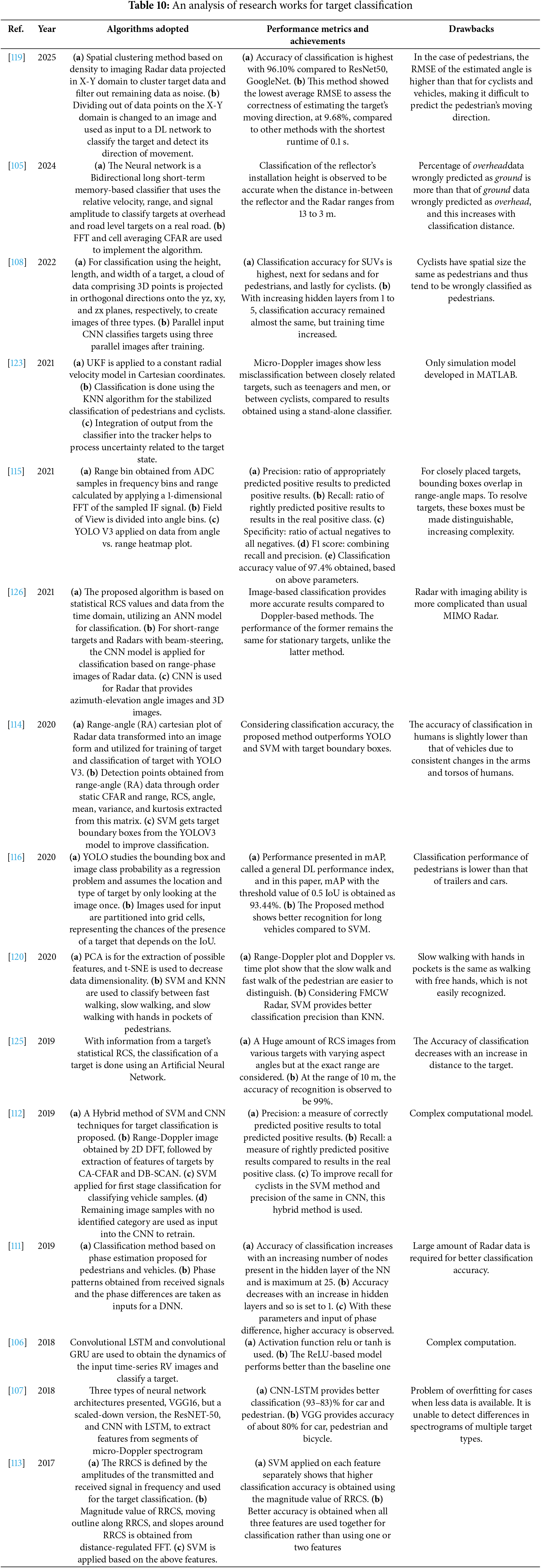
Table 11 contains an analysis of various algorithms used for target classification by automotive Radar.
6 Research Challenges and Future Scope
6.1 Challenges in Automotive Radar Signal Processing
The challenges faced in the signal processing of automotive Radar are explained in brief.
1. Interference—The introduction of more radar-fitted vehicles on the road leads to interference, such as self-interference originating from Radar signals reflected by the vehicle and radome, cross-interference from separate radars on the same vehicle, and cross-interference from Radars on another vehicle. Based on the waveforms, these are primarily FMCW-FMCW and FMCW-PMCW interference, and the interference level depends on the separation between Radars, beam pattern, and signal processing method. Interferences increase the likelihood of false alarms and obscure actual targets.
Solution: Methods like matched filtering for reducing FMCW waveform interference, and CDMA for reducing PMCW waveform interference are used. Recently, neural network-based mitigation methods have been studied.
2. High resolution—Automotive Radar is required to obtain information on the surrounding targets and classify them. For this purpose, high resolution is required in range, Doppler, elevation, and azimuth angles. High resolution is obtained using 2D-FFT in the range-Doppler domain, increasing the processor cost.
Solution: To maintain a balance between angular resolution and unambiguous field of view, in uniform rectangular arrays (URA), the resolution and field of view are monitored by horizontal and vertical antenna spacings. More research is underway to properly calibrate the array after vehicle integration and throughout Radar’s lifespan.
3. Estimation of parameters in Multipath and clutter scenarios—The operation scenario includes various targets like pedestrians, vehicles, animals, bridges, road structures, etc. Automotive Radar has to operate accurately to detect, track, and classify every target even in the presence of multipath propagation in urban road scenarios. The multi-path effect increases false alarms. The tracking of low-altitude targets, such as vehicles, is affected mainly by ground clutter.
Solution: Radar detection methods, based on the Convolutional Neural Network, can be used for complex clutter conditions.
4. Multi-target detection and ghost object removal—The detection of multiple targets is a difficult task as it involves proper clustering of Radar data associated with a specific target and tracking the position of every target in motion. Multi-target tracking algorithms can be applied to track the positions of multiple targets continuously. Sometimes, multiple radar reflections of the Radar signal produce ghost targets, i.e., targets which are not present.
Solution: To eliminate such an ambiguity, neural network-based classifiers can be used.
5. Detection in low SNR environments-Radars can usually operate under low SNR environments, like weather conditions with fog or snow. But in very adverse conditions, especially for automotive purposes, detection problems may occur.
Solution: During extreme bad weather conditions, continuous wave Radars with longer observation time are required for high range detection and range resolution.
6. Real-time constraints in embedded processing. The Operation of automotive Radar is a time-critical process. It is designed to detect and track targets, update target positions, and monitor the surrounding environment, all within a strict time duration, failing which can lead to accidents.
Solution: Adaptive signal processing and efficient algorithms with reduced computational complexities help to provide real-time, accurate Radar data.
7. Dataset scarcity and lack of standardization—Authorities such as EURO NCAP and the New Car Assessment Program for Southeast Asia (ASEAN NCAP) are present for automotive Radar standardization. However, a global standardization for regulations is still unavailable commercially. Additionally, the scarcity of real-time Radar data is another challenge to carry out further research in this field.
Solution: Country-specific Radar datasets are available for public use, which resolves this issue to some extent.
6.2 Innovations and Future Trends
The aim of research in automotive Radar has changed from hardware to millimeter-wave systems and RF signal processing methods. So, recent research has focused on digital modulation techniques, Cognitive Radar, Radar imaging, integrated sensing and communication, machine learning, and Quantum Radar. The research and evolution in this sector are outlined here in a brief [15]:
1. AI-driven Radar and Cognitive Radar-Target classification is required for risk assessment, sensing the resources, and finally, automated control. For target recognition and classification, a machine learning algorithm is usually adopted. In this aspect, a large, real or synthetic Radar dataset is required to be available for further work. Artificial Intelligence and Machine learning algorithms can be further utilized for localization, interference reduction, waveform design, and other specialized technologies. Like, Neural network such as CNN can be applied for the processing of non-clustered target detections [129]. In [130], a Deep Learning and Image Processing-based Height Estimator is applied to create a real time system that uses image data to obtain heights of buildings in the paths of unmanned aerial vehicles. Here, Google Street view images are used, which can be replaced with Radar images. An automated multi-path annotation method converts a conventional large Radar dataset into multi-path labeled data, on which deep learning-based signal processing is applied to challenges present in such scenarios [131]. A Cognitive Radar [132] can sense the environment, reason, and learn with the help of supervised techniques, and finally adapt its parameters to meet the changes in the scenario.
2. Radar imaging and 4D Radar—Imaging Radar is an innovative application, beneficial for measuring target RCS. Here, the echoes from the target are converted into digital form, sent to the data recorder for processing, and finally shown as an image. Range-azimuth imaging can be obtained by application of Super-Resolution Angular Spectra Estimation Network [133]. Another such technique is the 4D Radar [134,135] used to measure elevation and azimuth angles, range, and Doppler of the target, while providing high resolution and wider field-of-view. In the case of 4-dimensional imaging Radar, a waveform for MIMO-PMCW is better suited than the MIMO-FMCW model [136]. Coherent Radar networks can be applied to create a Radar image with better SNR and azimuth resolution and to obtain vectorial velocities of targets [137].
3. Integrated sensing and communication (ISAC)—In case of ISAC, the Radar and communication systems can coexist by either sharing the frequency spectrum, or by sharing the same hardware, or by using waveforms from the communication system for Radar functioning [138]. For understanding ISAC, in-depth knowledge of communication is also required. Like in [139], the structure of cell-free massive MIMO has been described for wireless communication networks and green communication methods.
4. Radar simulation and synthetic data for training—To compensate for the scarcity of real-time Radar data, synthetic data is artificially produced. This is very beneficial for the training process of the ML algorithms used for target tracking and classification.
5. Quantum Radar and metamaterial-based Radars—Recent innovations involve Quantum radar [140], which generates quantum entangled signals related to a reference signal present at the receiver. This Radar works better than conventional ones in low signal echoes and high noise, and is quite resilient to deception and electronic jamming.
6.3 Utility of Autonomous Driving
The main application of automotive Radar is to prevent accidents by using warning signals and automated safety functions, and thus achieve the Vision Zero objectives of zero deaths in traffic accidents. The main utilities of autonomous driving can be listed as
1. Safer Roads—As stated in the introduction, reducing road accidents is one of the most important motivations for autonomous vehicles. Automotive Radar sensors can perceive the environment better than human drivers; thus, driving errors like drunk driving and sleepy driving will be significantly reduced.
2. Improved traffic management and fuel efficiency—Automated vehicles will lead to better traffic management and reduced accident rates. Additionally, as vehicles are designed to enhance efficiency in acceleration and braking, fuel efficiency is expected to improve, resulting in reduced carbon emissions. Thus, helping the environment as a whole.
3. Free time for drivers—In levels 3, 4, and 5 of automation, most of the driving tasks will be done by automation, so drivers will have more time to spend on themselves. Accidents caused by drowsy drivers are a widespread incident, with automation, and drivers can rest on long rides.
4. Improved way of living—Even disabled persons and older citizens would be able to experience driving instead of relying on others.
5. Providing newer job opportunities—Job opportunities will be made in automobile, electronics, and software engineering, among others. With the mass production of automated cars, their price will eventually decrease and become more affordable for the general public.
7 Benchmark Datasets and Standards for Automotive Radar
Recent innovations in automotive Radar for target detection, tracking, and classification are being achieved by using ML algorithms. For the training data of the ML algorithms, a large Radar dataset is required, which contains an authentic and detailed description of the surrounding environment. Several Radar datasets are available publicly, and the important datasets are described concisely in this work. These datasets are presented in a comparative table in the following Table 12.
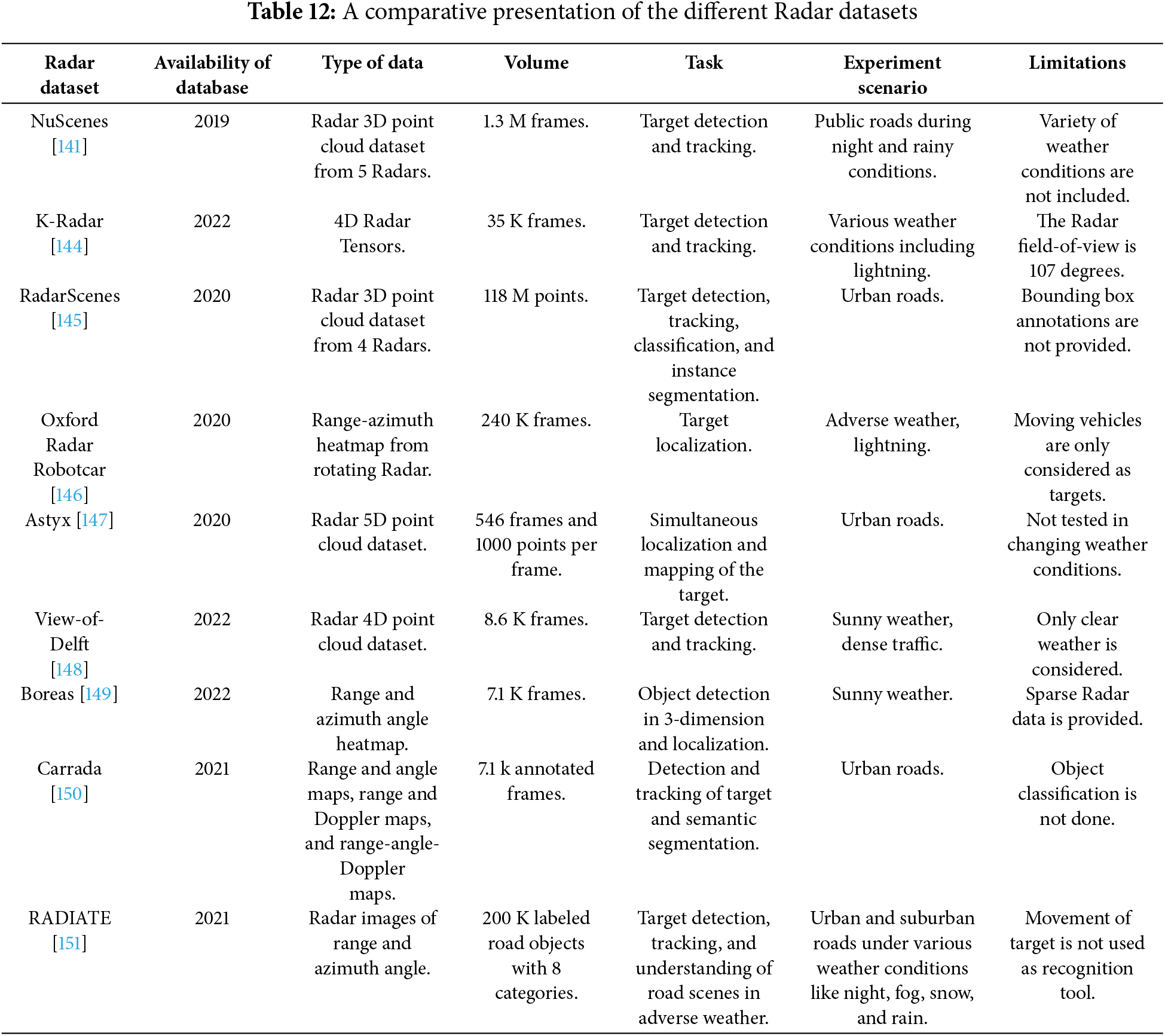
The nuScenes dataset [141] is the most well-known one that provides a large-scale Radar point cloud dataset obtained from 3-dimensional Radars [142]. This multimodal dataset offers 360-degree coverage of the entire surroundings, encompassing data from nighttime and rainy weather conditions, as well as features of objects and a detailed description of scenes. Stochastic geometry is used for modeling large automotive Radar networks in crowded urban scenarios, where interfering radar and clutter are assumed to be instances of a spatial stochastic point process [143].
The KAIST-Radar (K-Radar) [144] dataset is a 3-dimensional target detection dataset using the 4-dimensional Radar tensor, which describes a wide variety of scenarios. The 4-dimensional Radar tensor (DRT) consists of range, elevation, azimuth, Doppler, and power measurements, which help to preserve 3-dimensional spatial information for a proper 3-dimensional impression of targets.
Another dataset, the RadarScenes [145], is mainly available for models that have point-wise interpretations. This dataset is helpful for the development of ML algorithms used for mobile targets on the road, labeling them into 11 categories, including car, truck, train, bus, pedestrian, animal, and others.
The Oxford Radar Robotcar dataset [146] contains range and azimuth heatmap data used for target localization and fusion models of Lidar-Radar. This dataset comprises approximately 240,000 scans from a Navtech Radar, covering various weather conditions, lightning situations, and traffic scenarios.
In the Astyx dataset [147], the radar provides a 5-D point cloud data comprising range, elevation, azimuth, relative radial velocity, and a feedback magnitude. The feedback magnitude defines the reflection strength of the target detected by the Radar.
The main feature of the View-of-Delft (VoD) [148] automotive dataset is the (3 + 1D) Radar data, which includes range, elevation, and azimuth angles with Doppler, along with data from 3-dimensional Lidar and a stereo camera. The dataset has about 123,100+ 3-dimensional bounding box annotations of stagnant and moving objects. It also provides details of the semantic map and localization data of vehicles collected from urban road scenarios.
The Borreas [149] dataset for autonomous driving was accumulated by driving on a specific route map for one year. In this set, over 350 km of driving data are provided, including data collected under harsh weather conditions such as rain and snow. The sensors used here include a 360-degree Navtech Radar, a Lidar, and a camera. This dataset is utilized for object detection in 3D, metric localization, and odometry.
The Camera and Automotive Radar (Carrada) dataset [150] consists of synchronized Radar and camera data with range-angle-Doppler mapping. This is used as a basis for semantic segmentation with range-DOA or range-Doppler Radar presentations for target detection.
Radar Dataset In Adverse Weather (RADIATE) dataset [151] is used for target detection, tracking, and understanding of different road scenarios under various weather conditions like sunny, overcast, nighttime, rain, fog and snow. The unique feature of RADIATE is that eight road objects are labeled here, which include van, bus, truck, car, motorbike, cycle, group of pedestrians, and single pedestrian.
7.2 Standards and Evaluation Metrics
The standards and evaluation metrics are required for the performance evaluation of automotive Radar and comply with regulations. Two of the important standards defined are IEEE Standards Association P3116 [152], and European Telecommunications Standards Institute (ETSI) EN 302 264 [153]. The IEEE standard is used for the evaluation of performance metrics and testing techniques for applications of ADAS and the Automated Driving System (ADS). This standard defines the static parameter metrics, e.g., range, DOA, and velocity resolution, and the Field-of-View, and the dynamic parameter metrics like automotive Radar’s ability to resolve different targets in separate trajectories. The ETSI standard is applicable for short-range Radar with the operating frequency of 77 to 81 GHz. This contains technical specifications, tests for integrated transceivers, and separate transmit and receive systems.
The static evaluation metrics of automotive Radar include range, DOA, and Doppler resolution, Field-of-View, maximum and minimum detectable range, maximum and minimum detectable velocity, and RCS.
The dynamic evaluation metrics of automotive Radar include the probability of detection of targets, the ability to detect targets present in separate trajectories, detection in various adverse weather conditions, and the probability of false alarm rate.
This paper provides an overview of conventional automotive radar signal processing algorithms, highlighting their advantages and limitations for applicability to vehicular radar scenarios, and offers insights into new approaches for performance improvements. In particular, range-Doppler processing, target location and direction detection, tracking, and classification methods are discussed, specifically for high-resolution automotive Radars.
• Overview of Automotive Radar: A brief evolution of Automotive Radar and its application in the ADAS of autonomous vehicles and economic development is provided. A signal processing methodology is described, including the mathematical model for range and velocity measurement, to give information on the basic working principle of automotive Radar. A brief review of the different waveforms used in automotive Radar, along with their respective mathematical equations, is presented. A comparative analysis of these waveforms is presented in a tabular format to help determine the specific waveform for different functions. This article also examines common waveform interference problems from different types of radars, which are assumed to be the source of interference, and radars assumed to be the victims.
• Target detection and DOA estimation: The target detection signal processing architecture is briefly described. Various DOA evaluation algorithms, along with their numerical models, are studied, including Bartlett beamforming, MVDR beamforming, MUSIC, and ESPRIT. This article presents an extensive study of various relevant algorithms used by researchers for angle estimation. Analytical comparisons of all these algorithms are presented in tabular form, highlighting their merits and demerits. DOA estimation of a target is a primary requirement, and this section provides in-depth knowledge on this.
• Target tracking: After target detection, filtering and tracking techniques for obtaining target motion dynamics are required to stay informed about the target’s position. Target tracking involves a motion model for the target, filtering for target state estimation and data association, and track management. The filtering techniques mainly include the KF, the EKF, the UKF, and the Bayesian filter. Tracking targets is essential to avoid a collision, as in the ACC scenario. This paper provides an overview of various relevant algorithms that researchers use for tracking processes. Analytical comparisons of all these algorithms are presented in tabular form, highlighting their merits and demerits.
• Target recognition and classification: It is necessary to classify Radar signals into different categories based on their similarity to other signals. The algorithms used for this purpose include KNN and SVM, among others. This article provides detailed information on various relevant algorithms used by researchers for target classification, helping to better understand the process. Analytical comparisons of all these algorithms are presented in tabular form, highlighting their merits and demerits.
• Research challenges and future scope: Some of the major challenges for automotive Radar cases include interference mitigation, high resolution, parameter estimation in multipath scenarios, and target classification with Machine Learning. A brief knowledge of the various future scopes, like AI Radar, and integrated Radar and communication, is required to understand how the world is progressing in the automotive applications of Radar
• Benchmark datasets for automotive Radar: New research on automotive Radar is done mainly with the help of ML algorithms. For training these algorithms, a large amount of training data is required. An overview of the publicly available Radar datasets, highlighting their types of data and the tasks they can accomplish, is beneficial. Additionally, the standards and metrics for evaluating the parameters of automotive Radars are presented for further research.
As the vehicle industry moves towards full automation, various challenges will arise, and innovative solutions will be researched. Improved signal processing techniques will be introduced to utilize automotive Radar efficiently. As per the Automotive Radar Market Size, Share, Analysis Report, this industry is predicted to reach US Dollars 22.83 billion by 2032. There is a vast global demand for ADAS technologies, and the dominant sensor for this is the automotive Radar. Hence, this extensive picture of Radar signal processing is of utmost importance. Automotive radar signal processing techniques, along with a comparative analysis of various waveforms, are summarized here to enhance understanding of the working principles. I have a detailed review of the target detection and various DOA estimation algorithms for you, which is a necessary piece of research on this topic. Along with conventional MUSIC and ESPRIT algorithms, innovative ones such as E-MUSIC, group-sparsity-based, DML-based, and digital beamforming techniques are reviewed, highlighting their benefits and a few complexities. After target positioning, real-time tracking of the target is necessary, for which various algorithms have been discussed here, along with comparison tables highlighting their respective advantages and disadvantages. The tracking filters, such as KF, EKF, and Bayesian filters, as well as improved versions, like SRCKF and track-before-detect methods, are studied. Also, the entire tracking method, with data associated with measuring tracks and track management, is discussed. Classification of targets is required in real road scenarios to avoid clutter and false targets. It has been observed that target recognition and classification using machine learning (ML) algorithms are becoming increasingly important research topics. Algorithms for this technology have been thoroughly discussed, along with their importance and limitations. For the training purpose of these ML algorithms, a large amount of training data is required to understand the Radar environment. Some databases are openly available for conducting new research. A survey of the radar datasets is presented here, which shows the type of data and the tasks they can accomplish. Standards and parameter metrics of automotive radar are also provided here. The challenges faced in the automotive Radar signal processing field have also been described here to aid in further work to overcome them. A comprehensive picture of the signal processing technique typically used for automotive Radar is provided here to help better understand and inform future research in this area.
Acknowledgement: Pallabi Biswas and Samarendra Nath Sur acknowledge administrative and technical support from Sikkim Manipal Institute of Technology, Sikkim Manipal University, Sikkim, India.
Funding Statement: This work was supported in part by the National Science and Technology Council, Taiwan: NSTC 113-2410-H-030-077-MY2.
Author Contributions: Conceptualization: Samarendra Nath Sur and Rabindranath Bera; Investigation: Pallabi Biswas and Samarendra Nath Sur; Methodology: Rabindranath Bera, Samarendra Nath Sur and Chun-Ta Li; Supervision: Samarendra Nath Sur and Rabindranath Bera; Visualization: Pallabi Biswas and Agbotiname Lucky Imoize; Writing—original draft: Pallabi Biswas, Samarendra Nath Sur and Agbotiname Lucky Imoize; Writing—review and editing: Samarendra Nath Sur, Agbotiname Lucky Imoize and Chun-Ta Li. All authors reviewed the results and approved the final version of the manuscript.
Availability of Data and Materials: Data sharing not applicable to this article as no datasets were generated during the current study.
Ethics Approval: Not required.
Conflicts of Interest: The authors declare no conflicts of interest to report regarding the present study.
Abbreviations
| ADAS | Advanced Driver Assistance System |
| ACC | Adaptive Cruise Control |
| AEB | Automotive Emergency Braking |
| LRR | Long Range Radar |
| MRR | Medium Range Radar |
| SRR | Short Range Radar |
| FMCW | Frequency Modulated Continuous Wave |
| SNR | Signal to Noise Ratio |
| DOA | Direction of Arrival |
| RCS | Radar Cross Section |
| MUSIC | Multiple Signal Classification |
| ESPRIT | Estimation of Signal Parameters via Rotational Invariance Technique |
| PMCW | Phase Modulated Continuous Wave |
| PRF | Pulse Repetition Frequency |
| MIMO | Multiple Input Multiple Output |
| TDM/FDM | Time Division Multiplexing/Frequency Division Multiplexing |
| DDM | Dopple Division Multiplexing |
| PSD | Power Spectral Density |
| CFAR | Constant False Alarm Rate |
| GOCA-CFAR | Greatest of Cell Averaging Constant False Alarm Rate |
| SOCA-CFAR | Smallest of Cell Averaging Constant False Alarm Rate |
| OS-CFAR | Order Static Constant False Alarm Rate |
| MVDR | Minimum Variance Distortionless Response |
| CS | Compressive Sensing |
| SVM | Support Vector Machine |
| CTR | Constant Turn Rate |
| CTRA | Constant Turn Rate and Acceleration |
| KF | Kalman filter |
| EKF | Extended Kalman filter |
| UKF | Unscented Kalman filter PDF Probability Density Function |
| CKF/SRCKF | Cubature Kalman Filter/Square root Cubature Kalman Filter |
| JPDAF | Joint Probabilistic Data Association Filter |
| DRP | Doppler Range Processing |
| PD | Probability of Detection |
| SDR | Signal to Disturbance Ratio |
| RMSE | Root Mean Square Error |
| KNN | K-Nearest Neighbor |
| LSTM | Long Short Term Memory |
| CNN | Convolutional Neural Network |
| PCA | Principal Component Analysis |
References
1. Sur SN, Bera S, Bera R, Bhaskar D, Shome S. Spread spectrum radar for vehicular application. In: 2018 IEEE MTT-S International Microwave and RF Conference (IMaRC). Kolkata, India: IEEE; 2018. p. 1–4. [Google Scholar]
2. World Health Organization. Global Status Report on Road Safety. Geneva: World Health Organization; 2023. [cited 2025 Feb 1]. Available from: https://www.who.int/publications/i/item/global-status-report-on-road-safety-2023. [Google Scholar]
3. Kukkala VK, Tunnell J, Pasricha S, Bradley T. Advanced driver-assistance systems: a path towards autonomous vehicles. IEEE Consum Electron Mag. 2018;7(5):18–25. doi:10.1109/mce.2018.2828440. [Google Scholar] [CrossRef]
4. Giuffrida L, Masera G, Martina M. A survey of automotive radar and lidar signal processing and architectures. Chips. 2023;2(4):243–61. doi:10.3390/chips2040015. [Google Scholar] [CrossRef]
5. Barbosa FM, Osório FS. Camera-radar perception for autonomous vehicles and ADAS: concepts, datasets and metrics. arXiv:2303.04302. 2023. [Google Scholar]
6. Alland S, Stark W, Ali M, Hegde M. Interference in automotive radar systems. IEEE Signal Process Mag. 2019;36(5):45–59. [Google Scholar]
7. Yan B, Roberts IP. Advancements in millimeter-wave radar technologies for automotive systems: a signal processing perspective. Electronics. 2025;14(7):1436. doi:10.3390/electronics14071436. [Google Scholar] [CrossRef]
8. Waldschmidt C, Hasch J, Menzel W. Automotive radar—from first efforts to future systems. IEEE J Microw. 2021;1(1):135–48. doi:10.1109/jmw.2020.3033616. [Google Scholar] [CrossRef]
9. Magosi ZF, Eichberger A. A novel approach for simulation of automotive radar sensors designed for systematic support of vehicle development. Sensors. 2023;23(6):3227. doi:10.3390/s23063227. [Google Scholar] [PubMed] [CrossRef]
10. Abd El-Hameed AS, Ouf EG, Elboushi A, Seliem AG, Izumi Y. An improved performance radar sensor for K-band automotive radars. Sensors. 2023;23(16):7070. doi:10.3390/s23167070. [Google Scholar] [PubMed] [CrossRef]
11. Patole S, Torlak M, Wang D, Ali M. Automotive radars: a review of signal processing techniques. IEEE Signal Process Mag. 2017;34(2):22–35. doi:10.1109/msp.2016.2628914. [Google Scholar] [CrossRef]
12. Loeffler A, Zergiebel R, Wache J, Mejdoub M. Advances in automotive radar for 2023. In: 2023 24th International Radar Symposium (IRS). Berlin, Germany; 2023. p. 1–8. [Google Scholar]
13. Tavanti E, Rizik A, Fedeli A, Caviglia DD, Randazzo A. A short-range FMCW radar-based approach for multi-target human-vehicle detection. IEEE Trans Geosci Remote Sens. 2022;60:1–16. doi:10.1109/tgrs.2021.3138687. [Google Scholar] [CrossRef]
14. Händel C, Konttaniemi H, Autioniemi M. State-of-the-Art Review on Automotive Radars and Passive Radar Reflectors. Arctic Challenge Research Project; 2018. [cited 2024 Dec 1]. Available from: https://urn.fi/URN:ISBN:978-952-316-223-5. [Google Scholar]
15. Engels F, Heidenreich P, Wintermantel M, Stäcker L, Kadi MA, Zoubir AM. Automotive radar signal processing: research directions and practical challenges. IEEE J Sel Top Signal Process. 2021;15(4):865–78. doi:10.1109/jstsp.2021.3063666. [Google Scholar] [CrossRef]
16. Bera S, Sur SN, Singh AK, Bera R. RCS measurement and ISAR imaging radar in VHF/UHF radio channels. Int J Remote Sens. 2024;45(7):2159–81. doi:10.1080/01431161.2024.2326533. [Google Scholar] [CrossRef]
17. Bilik I, Longma O, Villeval S, Tabrikian J. The rise of radar for autonomous vehicles: signal processing solutions and future research directions. IEEE Signal Process Mag. 2019;36(5):20–31. doi:10.1109/msp.2019.2926573. [Google Scholar] [CrossRef]
18. SAE International. SAE J3016 Update; 2021. [cited 2025 Mar 13]. Available from: https://www.sae.org/blog/sae-j3016-update. [Google Scholar]
19. Malaquin C, Bonnabel A. Radar and Wireless for Automotive: Market and Technology Trends 2019; 2019. [cited 2025 Feb 1]. Available from: https://medias.yolegroup.com/uploads/2019/03/YD19009_Radar_and_Wireless_for_Automotive_2019_Sample-2.pdf. [Google Scholar]
20. Srivastav A, Mandal S. Radars for autonomous driving: a review of deep learning methods and challenges. IEEE Access. 2023;11:1–22. doi:10.1109/access.2023.3312382. [Google Scholar] [CrossRef]
21. Gerstmair M, Melzer A, Onic A, Huemer M. On the safe road towards autonomous driving. IEEE Signal Process Mag. 2019;36(5):60–99. [Google Scholar]
22. Venon A, Dupuis Y, Vasseur P, Merriaux P. Millimeter wave FMCW RADARs for perception, recognition and localization in automotive applications: a survey. IEEE Trans Intell Veh. 2022;7(3):533–55. doi:10.1109/tiv.2022.3167733. [Google Scholar] [CrossRef]
23. Gamba J. Radar signal processing for autonomous driving. In: Signals and communication technology. Singapore: Springer Nature Singapore Pte Ltd.; 2020. [Google Scholar]
24. Sun S, Zhang YD. 4D automotive radar sensing for autonomous vehicles: a sparsity-oriented approach. IEEE J Sel Top Signal Process. 2021;15(4):879–91. doi:10.1109/jstsp.2021.3079626. [Google Scholar] [CrossRef]
25. Thornton CE, Howard WW, Buehrer RM. Online learning-based waveform selection for improved vehicle recognition in automotive radar. In: ICASSP 2023–2023 IEEE International Conference on Acoustics, Speech and Signal Processing (ICASSP). Greece: Rhodes Island; 2023. p. 1–5. [Google Scholar]
26. Ramasubramanian K, Ginsburg B. AWR1243 Sensor: Highly Integrated 76-81 GHz Radar Front-End for Emerging ADAS Applications. Texas Instruments; 2017. [cited 2025 Feb 1]. Available from: https://www.ti.com/lit/wp/spyy005/spyy005.pdf. [Google Scholar]
27. Hakobyan G, Yang B. High-performance automotive radar: a review of signal processing algorithms and modulation schemes. IEEE Signal Process Mag. 2019;36(5):32–44. doi:10.1109/msp.2019.2911722. [Google Scholar] [CrossRef]
28. Caffa M, Biletta F, Maggiora R. Binary-phase vs. frequency modulated radar measured performances for automotive applications. Sensors. 2023;23(11):5271. doi:10.3390/s23115271. [Google Scholar] [PubMed] [CrossRef]
29. Kahlert M, Fei T, Tebruegge C, Gardill M. Stepped-frequency PMCW waveforms for automotive radar applications. IEEE Trans Radar Syst. 2025;3:233–45. doi:10.1109/trs.2025.3528773. [Google Scholar] [CrossRef]
30. Shome S, Bera R, Maji B, Sur SN, Bera S. Embedded digital MIMO radar using SDR for target detection and RCS measurement. IETE J Res. 2016;62(1):100–5. doi:10.1080/03772063.2015.1084244. [Google Scholar] [CrossRef]
31. Sun S, Petropulu AP, Poor HV. MIMO radar for advanced driver-assistance systems and autonomous driving. IEEE Signal Process Mag. 2020;37(4):98–117. doi:10.1109/msp.2020.2978507. [Google Scholar] [CrossRef]
32. Uysal F, Sanka S. Mitigation of automotive radar interference. In: 2018 IEEE Radar Conference (RadarConf18). Oklahoma City, OK, USA: IEEE; 2018. [Google Scholar]
33. Sur SN, Bera S, Bera R, Shome S. Spread spectrum radar for target characterization. Telecommun Radio Eng. 2019;78(14):1223–31. [Google Scholar]
34. Tamang ND, Sur SN, Bera S, Bera R. A review on spread spectrum radar. In: Advances in electronics, communication and computing: ETAEERE-2016. Singapore: Springer; 2017. p. 653–64 doi:10.1007/978-981-10-4765-7_68. [Google Scholar] [CrossRef]
35. Sur SN, Bera S, Singh AK, Shome S, Bera R, Maji B. Polyphase coded radar for target characterization in the open range environment. Measurement. 2021;167:108247. doi:10.1016/j.measurement.2020.108247. [Google Scholar] [CrossRef]
36. Mazher KU, Graff A, González-Prelcic N, Heath RW. Automotive radar interference characterization: FMCW or PMCW? In: ICASSP 2024–2024 IEEE International Conference on Acoustics, Speech and Signal Processing (ICASSP). Seoul, Republic of Korea; 2024. p. 13406–10. [Google Scholar]
37. Chen S, Klemp M, Taghia J, Kühnau U, Pohl N, Martin R. Improved target detection through DNN-based multi-channel interference mitigation in automotive radar. IEEE Trans Radar Syst. 2023;1:75–89. doi:10.1109/trs.2023.3279013. [Google Scholar] [CrossRef]
38. Kazazi J, Kamarei M, Fakharzadeh M. RD-CFAR: fast and accurate constant false alarm rate algorithm for automotive radar application. TechRxiv. 2025 Feb 07. doi:10.36227/techrxiv.173895066.68496282/v1. [Google Scholar] [CrossRef]
39. Zhang J, Fang C, Zheng Q, Tong Z. A novel method for micro-motion target detection and ghost track suppression in automotive radar. IET Conf Proc. 2024;2023(47):883–8. doi:10.1049/icp.2024.1203. [Google Scholar] [CrossRef]
40. Kazazi J, AleMohammad SMM, Kamarei M. U-Net-based automotive radar target detection and recognition. In: 2024 32nd International Conference on Electrical Engineering (ICEE). Tehran, Iran; 2024. p. 1–5. [Google Scholar]
41. Cho S, Song H, You KJ, Shin HC. A new direction-of-arrival estimation method using automotive radar sensor arrays. Int J Distrib Sens Netw. 2017;13(6):155014771771362. doi:10.1177/1550147717713628. [Google Scholar] [CrossRef]
42. Sim H, Lee S, Kang S, Kim SC. Enhanced DOA estimation using linearly predicted array expansion for automotive radar systems. IEEE Access. 2019;7:47714–27. doi:10.1109/access.2019.2910120. [Google Scholar] [CrossRef]
43. Xu S, Wang J, Yarovoy A. Super resolution DOA for FMCW automotive radar imaging. In: IEEE Conference on Antenna Measurements & Applications (CAMA). Sweden: IEEE; 2018. p. 1–4. [Google Scholar]
44. Sun R, Suzuki K, Owada Y, Takeda S, Umehira M, Wang X, et al. A millimeter-wave automotive radar with high angular resolution for identification of closely spaced on-road obstacles. Sci Rep. 2023;13(1):1–15. doi:10.1038/s41598-023-30406-4. [Google Scholar] [PubMed] [CrossRef]
45. Li Y, Zhang C, Song Y, Huang Y. Enhanced beamspace MUSIC for cost-effective FMCW automotive radar. IET Radar, Sonar Navig. 2020;14(2):257–67. [Google Scholar]
46. Maisto MA, Dell’Aversano A, Brancaccio A, Russo I, Solimene R. A computationally light MUSIC based algorithm for automotive RADARs. IEEE Trans Comput Imaging. 2024;10:446–60. doi:10.1109/tci.2024.3369412. [Google Scholar] [CrossRef]
47. Kahlert M, Xu L, Fei T, Gardill M, Sun S. High-resolution DOA estimation using single-snapshot music for automotive radar with Mixed-ADC allocations. In: 2024 IEEE 13rd Sensor Array and Multichannel Signal Processing Workshop (SAM). Corvallis, OR, USA; 2024. p. 1–5. doi:10.1109/sam60225.2024.10636418. [Google Scholar] [CrossRef]
48. Lee S, Yoon YJ, Lee JE, Sim H, Kim SC. Two-stage DOA estimation method for low SNR signals in automotive radars. IET Radar Sonar Navig. 2017;11(11):1613–9. [Google Scholar]
49. Shao M, Fan Y, Zhang Y, Zhang Z, Zhao J, Zhang B. A novel gridless non-uniform linear array direction of arrival estimation approach based on the improved alternating descent conditional gradient algorithm for automotive radar system. Remote Sens. 2025;17(2):303. doi:10.3390/rs17020303. [Google Scholar] [CrossRef]
50. Zaherfekr A, Ghoreishian MJ, Ebrahimzadeh A. DOA estimation in FMCW automotive radars with interference: ML and VMD approaches. In: 2024 11th International Symposium on Telecommunications (IST). Tehran, Iran; 2024. p. 795–800. [Google Scholar]
51. Karim BA, Ali HK. Computationally efficient MUSIC-based DOA estimation algorithm for FMCW Radar. J Electr Sci Technol. 2023;21(1):100192. doi:10.1016/j.jnlest.2023.100192. [Google Scholar] [CrossRef]
52. Van Trees HL. Optimum array processing: Part IV of detection, estimation, and modulation theory. New York, NY, USA: John Wiley & Sons; 2002. [Google Scholar]
53. Capon J. High-resolution frequency-wavenumber spectrum analysis. Proc IEEE. 1969;57(8):1408–18. doi:10.1109/proc.1969.7278. [Google Scholar] [CrossRef]
54. Schmidt R. Multiple emitter location and signal parameter estimation. IEEE Trans Antennas Propag. 1986;34(3):276–80. doi:10.1109/tap.1986.1143830. [Google Scholar] [CrossRef]
55. Roy R, Kailath T. ESPRIT-estimation of signal parameters via rotational invariance techniques. IEEE Trans Acoust Speech Signal Process. 1989;37(7):984–95. doi:10.1109/29.32276. [Google Scholar] [CrossRef]
56. Mehta P, Appaiah K, Velmurugan R. Robust direction-of-arrival estimation using array feedback beamforming in low SNR scenarios. IEEE Access. 2023;11:80647–55. doi:10.1109/access.2023.3300709. [Google Scholar] [CrossRef]
57. Godara LC. Application of antenna arrays to mobile communications. II. Beam-forming and direction-of-arrival considerations. Proc IEEE. 1997;85(8):1195–245. doi:10.1109/5.622504. [Google Scholar] [CrossRef]
58. Zhang W, Wang P, He N, He Z. Super resolution DOA based on relative motion for FMCW automotive Radar. IEEE Trans Veh Technol. 2020;69(8):8698–709. doi:10.1109/tvt.2020.2999640. [Google Scholar] [CrossRef]
59. Yuan S, Fioranelli F, Yarovoy AG. Vehicular-motion-based DOA estimation with a limited amount of snapshots for automotive MIMO Radar. IEEE Trans Aerosp Electr Syst. 2023;59(6):7611–25. doi:10.1109/taes.2023.3291335. [Google Scholar] [CrossRef]
60. Amani N, Jansen F, Filippi A, Ivashina MV, Maaskant R. Sparse automotive MIMO radar for super-resolution single snapshot DOA estimation with mutual coupling. IEEE Access. 2021;9:146822–9. doi:10.1109/access.2021.3122967. [Google Scholar] [CrossRef]
61. Xu Z, Chen Y, Zhang P. A sparse uniform linear array DOA estimation algorithm for FMCW radar. IEEE Signal Process Lett. 2023;30:823–7. doi:10.1109/lsp.2023.3292739. [Google Scholar] [CrossRef]
62. Moussa A, Liu W. A two-stage sparsity-based method for location and doppler estimation in bistatic automotive radar. In: 2023 IEEE Statistical Signal Processing Workshop (SSP). Hanoi, Vietnam: IEEE; 2023. p. 487–91. doi:10.1109/ssp53291.2023.10207941. [Google Scholar] [CrossRef]
63. Moussa A, Liu W, Zhang YD, Greco MS. Multi-target location and doppler estimation in multistatic automotive radar applications. IEEE Trans Radar Syst. 2024;2(2):215–25. doi:10.1109/trs.2024.3362706. [Google Scholar] [CrossRef]
64. Moussa A, Liu W. Estimation of doppler, range, and direction of targets in wideband bistatic automotive radar. In: ICASSP, 2025–2025 IEEE International Conference on Acoustics, Speech and Signal Processing (ICASSP). Hyderabad, India; 2025. p. 1–5. [Google Scholar]
65. Correas-Serrano A, González-Huici MA. Experimental evaluation of compressive sensing for DoA estimation in automotive radar. In: 19th International Radar Symposium (IRS). Bonn, Germany: IEEE; 2018. p. 1–10. [Google Scholar]
66. Zheng L, Long J, Lops M, Liu F, Hu X, Zhao C. Detection of ghost targets for automotive radar in the presence of multipath. IEEE Trans Signal Process. 2024;72(3):2204–20. doi:10.1109/tsp.2024.3384750. [Google Scholar] [CrossRef]
67. Sim H, Kang S, Lee S, Kim SC. Improved DOA estimation method by distinction of different transmit signals in automotive MIMO frequency-modulated continuous wave radar systems. IET Radar Sonar Navig. 2020;14(8):1135–42. doi:10.1049/iet-rsn.2019.0634. [Google Scholar] [CrossRef]
68. Wu Y, Li C, Hou YT, Lou W. Real-time DOA estimation for automotive radar. In: 18th European Radar Conference (EuRAD). London, UK: IEEE; 2022. p. 437–40. [Google Scholar]
69. Wu Y, Li C, Hou YT, Lou W. A real-time super-resolution doa estimation algorithm for automotive radar sensor. IEEE Sensors J. 2024;24(22):37947–61. doi:10.1109/jsen.2024.3462350. [Google Scholar] [CrossRef]
70. Jauch A, Meinl F, Blume H. DoA estimation in automotive MIMO radar with sparse array via fast variational bayesian method. In: 2023 IEEE Conference on Antenna Measurements and Applications (CAMA); Genoa, Italy; 2023. p. 892–7. [Google Scholar]
71. Jauch A, Meinl F, Blume H. Hardware-friendly variational bayesian method for DoA estimation in automotive MIMO radar. In: 2024 9th International Conference on Frontiers of Signal Processing (ICFSP). Paris, France; 2024. p. 174–8. [Google Scholar]
72. Fuchs J, Gardill M, Lübke M, Dubey A, Lurz F. A machine learning perspective on automotive radar direction of arrival estimation. IEEE Access. 2022;10:6775–97. doi:10.1109/access.2022.3141587. [Google Scholar] [CrossRef]
73. Song Y, Li Y, Zhang C, Huang Y. Data driven low-complexity DOA estimation for ultra-short range automotive radar. In: 2019 IEEE International Workshop on Signal Processing Systems (SiPS). Nanjing, China: IEEE; 2019. p. 313–7. doi:10.1109/sips47522.2019.9020602. [Google Scholar] [CrossRef]
74. Chen M. Short-range target tracking using high-resolution automotive radars [doctoral dissertation]. Hamilton, ON, Canada: McMaster University; 2024. [cited 2025 Jan 3]. Available from: http://hdl.handle.net/11375/29759. [Google Scholar]
75. Shamsfakhr F, Macii D, Palopoli L, Corrà M, Ferrari A, Fontanelli D. A multi-target detection and position tracking algorithm based on mmWave-FMCW radar data. Measurement. 2024;234(11):114797. doi:10.1016/j.measurement.2024.114797. [Google Scholar] [CrossRef]
76. Zhou T, Yang M, Jiang K, Wong H, Yang D. MMW radar-based technologies in autonomous driving: a review. Sensors. 2020;20(24):7283. [Google Scholar] [PubMed]
77. Eltrass A, Khalil M. Automotive radar system for multiple-vehicle detection and tracking in urban environments. IET Intell Trans Syst. 2018;12(8):783–92. doi:10.1049/iet-its.2017.0370. [Google Scholar] [CrossRef]
78. Khalil M, Eltrass AS, Elzaafarany O, Galal B, Walid K, Tarek A, et al. An improved approach for multi-target detection and tracking in automotive radar systems. In: International Conference on Electromagnetics in Advanced Applications (ICEAA). Cairns, QLD, Australia: IEEE; 2016. p. 480–3. [Google Scholar]
79. Uysal F, Aubry PJ, Yarovoy A. Accurate target localization for automotive radar. In: 2019 IEEE Radar Conference (RadarConf). Boston, MA, USA: IEEE; 2019. p. 1–5. [Google Scholar]
80. Li Y, Liang C, Lu M, Hu X, Wang Y. Cascaded Kalman filter for target tracking in automotive radar. J Eng. 2018;2019(19):6264–7. doi:10.1049/joe.2019.0159. [Google Scholar] [CrossRef]
81. Song S, Wu J, Zhang S, Liu Y, Yang S. Research on target tracking algorithm using millimeter-wave radar on curved road. Math Probl Eng. 2020;2020(4):1–21. doi:10.1155/2020/3749759. [Google Scholar] [CrossRef]
82. Wang CL, Xiong X, Liu HJ. Target tracking algorithm of automotive radar based on iterated square-root CKF. J Phys: Conf Ser. 2018;976:012010. doi:10.1088/1742-6596/976/1/012010. [Google Scholar] [CrossRef]
83. Liu Q, Song K, Xie H, Meng C. Research on invalid target filtering and target tracking algorithm optimization in millimeter-wave radar technology. In: SAE Technical Paper Series. Xi’an, China: SAE International; 2025. doi:10.4271/2025-01-7035. [Google Scholar] [CrossRef]
84. Tan B, Ma Z, Zhu X, Li S, Zheng L, Huang L, et al. Tracking of multiple static and dynamic targets for 4D automotive millimeter-wave radar point cloud in urban environments. Remote Sens. 2023;15(11):2923. doi:10.3390/rs15112923. [Google Scholar] [CrossRef]
85. Koloushani M, Naghsh MM, Reza Taban M, Karbasi SM. Multitarget tracking in the presence of velocity ambiguity for automotive radar. In: ICASSP 2024–2024 IEEE International Conference on Acoustics, Speech and Signal Processing (ICASSP). Seoul, Republic of Korea; 2024. p. 8851–5. [Google Scholar]
86. Wu Q, Chen L, Li Y, Wang Z, Yao S, Li H. Reweighted robust particle filtering approach for target tracking in automotive radar application. Remote Sens. 2022;14(21):5477. doi:10.3390/rs14215477. [Google Scholar] [CrossRef]
87. Chen Y, Wang Y, Qu F, Li W. A graph-based track-before-detect algorithm for automotive radar target detection. IEEE Sens J. 2021;21(5):6587–99. doi:10.1109/jsen.2020.3042079. [Google Scholar] [CrossRef]
88. Li W, Miao Q, Yuan Y, Tian Y, yi W, Teh K. Automotive radar multi-frame track-before-detect algorithm considering self-positioning errors. IEEE Trans Intell Transp Syst. 2025;1–16. doi:10.1109/tits.2025.3565733. [Google Scholar] [CrossRef]
89. Miao Q, Li PMM, Li W, Yi W. Motion compensation based track-before-detect methods for automotive radar system. In: 2024 Photonics & Electromagnetics Research Symposium (PIERS). Chengdu, China: IEEE; 2024. p. 1–10. [Google Scholar]
90. Jacobs L, Veelaert P, Steendam H, Philips W. On the accuracy of automotive radar tracking. In: 2023 IEEE 97th Vehicular Technology Conference (VTC2023-Spring). Florence, Italy: IEEE; 2023. p. 1–6. [Google Scholar]
91. Manjunath A, Liu Y, Henriques B, Engstle A. Radar based object detection and tracking for autonomous driving. In: IEEE MTT-S International Conference on Microwaves for Intelligent Mobility (ICMIM). Munich, Germany: IEEE; 2018. p. 1–4. [Google Scholar]
92. Held P, Steinhauser D, Koch A, Brandmeier T, Schwarz UT. A novel approach for model-based pedestrian tracking using automotive radar. IEEE Trans Intell Trans Syst. 2022;23(7):7082–95. doi:10.1109/tits.2021.3066680. [Google Scholar] [CrossRef]
93. Huang F, Zhou J, Zhao X. An improved multi-target tracking algorithm for automotive radar. J Phys: Conf Ser. 2021;1971(1):012076. doi:10.1088/1742-6596/1971/1/012076. [Google Scholar] [CrossRef]
94. Honer J, Kaulbersch H. Bayesian extended target tracking with automotive radar using learned spatial distribution models. In: IEEE International Conference on Multisensor Fusion and Integration for Intelligent Systems (MFI). Karlsruhe, Germany: IEEE; 2020. p. 316–22. [Google Scholar]
95. Tian F, Guo X, Fu W. Target tracking algorithm based on adaptive strong tracking extended kalman filter. Electronics. 2024;13(3):652. doi:10.3390/electronics13030652. [Google Scholar] [CrossRef]
96. de Ramos DC, Ferreira LR, Santos MMD, Teixeira ELS, Yoshioka LR, Justo JF, et al. Evaluation of cluster algorithms for radar-based object recognition in autonomous and assisted driving. Sensors. 2024;24(22):1–31. [Google Scholar]
97. Ren J, Zhang L, Liu J. Research and implementation of 77 GHz automotive radar target detection technology. In: 2023 6th International Conference on Information Communication and Signal Processing (ICICSP). Xi’an, China; 2023. p. 517–21. [Google Scholar]
98. Xu L, Lien J, Li J. Doppler-range processing for enhanced high-speed moving target detection using LFMCW automotive radar. IEEE Trans Aerosp Electr Syst. 2021;58(1):568–80. doi:10.1109/taes.2021.3101768. [Google Scholar] [CrossRef]
99. Li Y, Li G, Liu Y, Zhang XP, He Y. A hybrid SVSF algorithm for automotive radar tracking. IEEE Trans Intell Trans Syst. 2022;23(9):15028–42. doi:10.1109/tits.2021.3136170. [Google Scholar] [CrossRef]
100. Tilly JF, Haag S, Schumann O, Weishaupt F, Duraisamy B, Dickmann J, et al. Detection and tracking on automotive radar data with deep learning. In: 2020 IEEE 23rd International Conference on Information Fusion (FUSION). Rustenburg, South Africa: IEEE; 2020. p. 1–7. [Google Scholar]
101. Cao X, Lan J, Li XR, Liu Y. Automotive radar-based vehicle tracking using data-region association. IEEE Trans Intell Trans Syst. 2022;23(7):8997–9010. doi:10.1109/tits.2021.3089676. [Google Scholar] [CrossRef]
102. Lindenmaier L, Aradi S, Bécsi T, Fekete B. Comparison of track management strategies in automotive track-to-track fusion algorithms. In: 2025 IEEE 23rd World Symposium on Applied Machine Intelligence and Informatics (SAMI). Stará Lesná, Slovakia: IEEE; 2025. [Google Scholar]
103. Ghatak G. Target tracking: statistics of successive successful target detection in automotive radar networks. arXiv:2411.18252. 2024. [Google Scholar]
104. Lee KC. Radar target recognition by machine learning of K-nearest neighbors regression on angular diversity RCS. ACES J. 2019;34(1):75–81. [Google Scholar]
105. Park C, Kwak S, Lee H, Lee S. Bidirectional LSTM-based overhead target classification for automotive radar systems. IEEE Trans Instrum Meas 2024;73(2):1–11. doi:10.1109/tim.2023.3343741. [Google Scholar] [CrossRef]
106. Kim S, Lee S, Doo S, Shim B. Moving target classification in automotive radar systems using convolutional recurrent neural networks. In: 26th European Signal Processing Conference (EUSIPCO). Rome, Italy: IEEE; 2018. p. 1482–6. [Google Scholar]
107. Angelov A, Robertson A, Murray-Smith R, Fioranelli F. Practical classification of different moving targets using automotive radar and deep neural networks. IET Radar Sonar Navig. 2018;12(10):1082–9. [Google Scholar]
108. Kwak S, Kim H, Kim G, Lee S. Multi-view convolutional neural network-based target classification in high-resolution automotive radar sensor. IET Radar Sonar Navig. 2022;17(1):15–26. doi:10.1049/rsn2.12320. [Google Scholar] [CrossRef]
109. Wen Q, Cao S. Radar range-doppler flow: a radar signal processing technique to enhance radar target classification. IEEE Trans Aerosp Electronic Syst. 2024;60(2):1519–29. doi:10.1109/taes.2023.3337757. [Google Scholar] [CrossRef]
110. Richter Y, Balal N, Pinhasi Y. Neural-network-based target classification and range detection by CW MMW radar. Remote Sens. 2023;15(18):4553. doi:10.3390/rs15184553. [Google Scholar] [CrossRef]
111. Lim S, Lee S, Yoon J, Kim SC. Phase-based target classification using neural network in automotive radar systems. In: IEEE Radar Conference (RadarConf). Boston, MA, USA: IEEE; 2019. p. 1–6. [Google Scholar]
112. Gao T, Lai Z, Mei Z, Wu Q. Hybrid SVM-CNN classification technique for moving targets in automotive FMCW radar system. In: 11th International Conference on Wireless Communications and Signal Processing (WCSP). Xi’an, China: IEEE; 2019. p. 1–6. [Google Scholar]
113. Lee S, Yoon YJ, Lee JE, Kim SC. Human-vehicle classification using feature-based SVM in 77-GHz automotive FMCW radar. IET Radar Sonar Navig. 2017;11(10):1589–96. doi:10.1049/iet-rsn.2017.0126. [Google Scholar] [CrossRef]
114. Kim W, Cho H, Kim J, Kim B, Lee S. Target classification using combined YOLO-SVM in high-resolution automotive FMCW radar. In: IEEE Radar Conference (RadarConf20). Florence, Italy: IEEE; 2020. p. 1–5. [Google Scholar]
115. Gupta S, Rai PK, Kumar A, Yalavarthy PK, Cenkeramaddi LR. Target classification by mmWave FMCW radars using machine learning on range-angle images. IEEE Sens J. 2021;21(18):19993–20001. doi:10.1109/jsen.2021.3092583. [Google Scholar] [CrossRef]
116. Kim W, Cho H, Kim J, Kim B, Lee S. YOLO-based simultaneous target detection and classification in automotive FMCW radar systems. Sensors. 2020;20(10):2897. doi:10.3390/s20102897. [Google Scholar] [PubMed] [CrossRef]
117. Sohail M, Khan AU, Sandhu M, Shoukat I, Jafri M, Shin H. Radar sensor based machine learning approach for precise vehicle position estimation. Sci Rep. 2023;13(1):13837. doi:10.1038/s41598-023-40961-5. [Google Scholar] [PubMed] [CrossRef]
118. Lamane M, Tabaa M, Klilou A. Classification of targets detected by mmWave radar using YOLOv5. Procedia Comput Sci. 2022;203(18):426–31. doi:10.1016/j.procs.2022.07.056. [Google Scholar] [CrossRef]
119. Lee H, Kwak S, Lee S. Multiple-output network for simultaneous target classification and moving direction estimation in automotive radar systems. Expert Syst Appl. 2025;259(10):125280. doi:10.1016/j.eswa.2024.125280. [Google Scholar] [CrossRef]
120. Senigagliesi L, Ciattaglia G, De Santis A, Gambi E. People walking classification using automotive radar. Electronics. 2020;9(4):588. doi:10.3390/electronics9040588. [Google Scholar] [CrossRef]
121. Chipengo U, Sligar AP, Canta SM, Goldgruber M, Leibovich H, Carpenter S. High fidelity physics simulation-based convolutional neural network for automotive radar target classification using micro-doppler. IEEE Access. 2021;9:82597–617. doi:10.1109/access.2021.3085985. [Google Scholar] [CrossRef]
122. Lee Y, Kim J, Kim S, Lee H, Lee S. Estimation of moving direction and size of vehicle in high-resolution automotive radar system. IEEE Trans Intell Trans Syst. 2024;25(7):7174–86. doi:10.1109/tits.2023.3339811. [Google Scholar] [CrossRef]
123. Dubey A, Santra A, Fuchs J, Lübke M, Weigel R, Lurz F. Integrated classification and localization of targets using bayesian framework in automotive radars. In: ICASSP 2021-IEEE International Conference on Acoustics, Speech and Signal Processing (ICASSP). Toronto, ON, Canada: IEEE; 2021. p. 4060–4. [Google Scholar]
124. Kanona MEA, Alias MY, Hassan MK, Mohamed KS, Khairi MHH, Hamdan M, et al. A machine learning based vehicle classification in forward scattering radar. IEEE Access. 2022;10(2):64688–700. doi:10.1109/access.2022.3183127. [Google Scholar] [CrossRef]
125. Cai X, Sarabandi K. A Machine learning based 77 GHz radar target classification for autonomous vehicles. In: 2019 IEEE International Symposium on Antennas and Propagation and USNC-URSI Radio Science Meeting. Atlanta, GA, USA: IEEE; 2019. p. 371–2. [Google Scholar]
126. Cai X, Giallorenzo M, Sarabandi K. Machine learning-based target classification for MMW radar in autonomous driving. IEEE Trans Intell Veh. 2021;6(4):678–89. doi:10.1109/tiv.2020.3048944. [Google Scholar] [CrossRef]
127. Duong S, Kahrizi D, Mettler S, Klöck C. Moving target classification with a dual automotive FMCW radar system using convolutional neural networks. In: 2021 21st International Radar Symposium (IRS). Berlin, Germany; 2021. p. 1–9. [Google Scholar]
128. Ulrich M, ser Glä C, Timm F. DeepReflecs: deep learning for automotive object classification with radar reflections. In: 2021 IEEE Radar Conference (RadarConf21). Atlanta, GA, USA; 2021. p. 1–6. [Google Scholar]
129. Kung YC, Zhou X, Shen H, Ahn J, Wang J. Convolutional neural networks for interpreting unclustered radar data in automotive applications. In: 2023 IEEE International Automated Vehicle Validation Conference (IAVVC). Austin, TX, USA; 2023. p. 1–6. [Google Scholar]
130. Pattanaik S, Imoize AL, Li CT, Francis SAJ, Lee CC, Roy DS. Data-driven diffraction loss estimation for future intelligent transportation systems in 6G networks. Mathematics. 2023;11(13):3004. doi:10.3390/math11133004. [Google Scholar] [CrossRef]
131. Danino S, Bilik I. Automatic multipath annotation for conventional automotive radar datasets. IEEE Sens J. 2024;24(8):13500–17. doi:10.1109/jsen.2024.3364497. [Google Scholar] [CrossRef]
132. Gurbuz SZ, Griffiths HD, Charlish A, Rangaswamy M, Greco MS, Bell K. An overview of cognitive radar: past, present, and future. IEEE Aerosp Electr Syst Mag. 2019;34(12):6–18. doi:10.1109/maes.2019.2953762. [Google Scholar] [CrossRef]
133. Zheng R, Sun S, Caesar H, Chen H, Li J. Redefining automotive radar imaging: a domain-informed 1D deep learning approach for high-resolution and efficient performance. 2024. doi:10.48550/arXiv.2406.07399. [Google Scholar] [CrossRef]
134. Fan L, Wang J, Chang Y, Li Y, Wang Y, Cao D. 4D mmWave radar for autonomous driving perception: a comprehensive survey. IEEE Trans Intell Veh. 2024;9(4):4606–20. doi:10.1109/tiv.2024.3380244. [Google Scholar] [CrossRef]
135. Chan PH, Shahbeigi Roudposhti S, Ye X, Donzella V. A noise analysis of 4D RADAR: robust sensing for automotive? IEEE Sens J. 2025;25(10):18291–301. doi:10.36227/techrxiv.24517249.v1. [Google Scholar] [CrossRef]
136. Sichani NK, Ahmadi M, Raei E, Alaee-Kerahroodi M, M.R. BS, Mehrshahi E, et al. Waveform selection for FMCW and PMCW 4D-imaging automotive radar sensors. In: 2023 IEEE Radar Conference (RadarConf23). San Antonio, TX, USA; 2023. p. 1–6. [Google Scholar]
137. Gottinger M, Hoffmann M, Christmann M, Schütz M, Kirsch F, Gulden P, et al. Coherent automotive radar networks: the next generation of radar-based imaging and mapping. IEEE J Microw. 2021;1(1):149–63. doi:10.1109/jmw.2020.3034475. [Google Scholar] [CrossRef]
138. Dong F, Wang W, Li X, Liu F, Chen S, Hanzo L. Joint beamforming design for dual-functional MIMO radar and communication systems guaranteeing physical layer security. IEEE Trans Green Commun Netw. 2023;7(1):537–49. doi:10.1109/tgcn.2022.3233863. [Google Scholar] [CrossRef]
139. Imoize AL, Obakhena HI, Anyasi FI, Sur SN. A review of energy efficiency and power control schemes in ultra-dense cell-free massive MIMO systems for sustainable 6G wireless communication. Sustainability. 2022;14(17):11100. doi:10.3390/su141711100. [Google Scholar] [CrossRef]
140. Maccone L, Ren C. Quantum radar. Phys Rev Lett. 2020;124:1–5. [Google Scholar]
141. Caesar H, Bankiti V, Lang AH, Vora S, Liong VE, Xu Q, et al. NuScenes: a multimodal dataset for autonomous driving. In: 2020 IEEE/CVF Conference on Computer Vision and Pattern Recognition (CVPR). Seattle, WA, USA: IEEE; 2020. p. 11618–28. [Google Scholar]
142. Muckenhuber S, Museljic E, Stettinger G. Performance evaluation of a state-of-the-art automotive radar and corresponding modeling approaches based on a large labeled dataset. J Intell Trans Syst. 2022;26(6):655–74. doi:10.1080/15472450.2021.1959328. [Google Scholar] [CrossRef]
143. Ram SS, Ghatak G. Emerging trends in radar: automotive radar networks. IEEE Aerosp Electron Syst Mag. 2025;40(6):54–9. doi:10.1109/maes.2025.3539254. [Google Scholar] [CrossRef]
144. Paek DH, Kong SH, TirtaWijaya K. K-radar: 4D radar object detection for autonomous driving in various weather conditions. In: 36th Conference on Neural Information Processing Systems (NeurIPS 2022) Track on Datasets and Benchmarks. New York, USA: Neurips; 2022. p. 1–8. [Google Scholar]
145. Schumann O, Hahn M, Scheiner N, Weishaupt F, Tilly JF, Dickmann J, et al. RadarScenes: a real-world radar point cloud data set for automotive applications. In: 2021 IEEE 24th International Conference on Information Fusion (FUSION). Sun City, South Africa: IEEE; 2021. p. 1–8. [Google Scholar]
146. Barnes D, Gadd M, Murcutt P, Newman P, Posner I. The oxford radar robotcar dataset: a radar extension to the oxford robotcar dataset. In: 2020 IEEE International Conference on Robotics and Automation (ICRA). Paris, France: IEEE; 2020. p. 6433–8. [Google Scholar]
147. Meyer M, Kuschk G. Automotive radar dataset for deep learning based 3D object detection. In: 2019 16th European Radar Conference (EuRAD). Paris, France: IEEE; 2019. p. 129–32. [Google Scholar]
148. Palffy A, Pool E, Baratam S, Kooij JFP, Gavrila DM. Multi-class road user detection with 3+1D radar in the view-of-delft dataset. IEEE Robot Autom Lett. 2022;7(2):4961–8. doi:10.1109/lra.2022.3147324. [Google Scholar] [CrossRef]
149. Burnett K, Yoon DJ, Wu Y, Li AZ, Zhang H, Lu S, et al. Boreas: a multi-season autonomous driving dataset. Int J Rob Res. 2023;42(1–2):33–42. doi:10.1177/02783649231160195. [Google Scholar] [CrossRef]
150. Ouaknine A, Newson A, Rebut J, Tupin F, Pérez P. CARRADA dataset: camera and automotive radar with range-angle-doppler annotations. In: 2020 25th International Conference on Pattern Recognition (ICPR). Milan, Italy: IEEE; 2021. p. 5068–75. [Google Scholar]
151. Sheeny M, De Pellegrin E, Mukherjee S, Ahrabian A, Wang S, Wallace A. RADIATE: a radar dataset for automotive perception in bad weather. In: 2021 IEEE International Conference on Robotics and Automation (ICRA). Xi’an, China: IEEE; 2021. p. 1–7. [Google Scholar]
152. Rafieinia F, Castro R, Wyglinski A, Mcnew J. Standard for automotive radar performance metrics and testing methods for advanced driver assistance systems (ADAS) and automated driving system(ADS) applications. IEEE; 2019. [cited 2025 Feb 1]. Available from: https://standards.ieee.org/ieee/3116/10712/. [Google Scholar]
153. Short Range Devices; Transport and Traffic Telematics (TTT); Short Range Radar equipment operating in the 77 to 81 GHz band. Harmonised Standard covering the essential requirements of article 3.2 of Directive 2014/53/EU; 2017. [cited 2025 Jan 3]. Available from: https://www.etsi.org/deliver/etsi_en/302200_302299/302264/02.01.01_30/en_302264v020101v.pdf. [Google Scholar]
Cite This Article
 Copyright © 2025 The Author(s). Published by Tech Science Press.
This work is licensed under a Creative Commons Attribution 4.0 International License , which permits unrestricted use, distribution, and reproduction in any medium, provided the original work is properly cited.
 Downloads
 Citation Tools