A New Extension Odd Generalized Exponential Model Using Type-II Progressive Censoring and Its Applications in Engineering and Medicine

1  Introduction

Researchers and statisticians have been focusing close attention to new normalized distributions in recent years due to their flexibility in statistical modeling and wide use in nearly all scientific domains. Marshall and Olkin [1] proposed adding a parameter to the survival function G¯(X)=1−G(X), where G(X) is the cumulative distribution function (CDF) of the baseline distribution, to define the exponentiated—G class of distributions based on Lehmann—type alternatives, see [2].

As per Gupta and Kundu, Gupta [3] explored the two-parameter generalized-exponential (GE) distribution, extending it from the exponential distribution with a Lehmann type I alternative. Numerous researchers have examined its characteristics and suggested comparisons with alternative distributions due to its widespread applications in modeling power system equipment, rainfall data, software reliability, animal behavior analysis, and various other fields.

Olabad conducted a series of studies [4–7] exploring various types of extended generalized logistic distributions, including type I extended forms [4], negatively skewed versions [5], symmetric distributions [6], and extended generalized exponential formulations [7], highlighting the flexibility of logistic-type models in capturing a wide range of distributional shapes.

Alizadeh et al. [8] further expanded this framework by introducing the Kumaraswamy odd log-logistic family, which demonstrated greater flexibility in modeling complex hazard shapes and tail behaviors in applied datasets. Cordeiro and de Castro [9] contributed by proposing a new family of generalized distributions through innovative transformation techniques, opening new directions for statistical inference and distribution theory. Similarly, Maiti [10] introduced the odd generalized exponential–exponential distribution, emphasizing its mathematical properties and usefulness in fitting real data.

Finally, Tahir et al. [11] introduced a new generalization of the odd generalized exponential family (OEGE−E) based on replacing x in the CDF of the model given by

FOGE−E(x,β,λ)=(1−e−λx)β,x>0,β>0,λ>0.(1)

where β,λ are positive parameters; by G(x,Λ)G¯(x,Λ) where G(x;Λ) and G¯(x,Λ) are the CDF and the survival function of parent distribution with a parameter vector Λ, respectively. So, the CDF of the OEGE family can be written as:

F(x;β,λ,Λ)=(1−e−λ(G(x;Λ)G¯(x;Λ))β(2)

and the probability density function (PDF) is given by:

f(x;β,λ,Λ)=βλg(x;Λ)G¯(x;Λ)e−λ(G(x;Λ))G¯(x;Λ)(1−e−λ(G(x;Λ))G¯(x;Λ))β−1,(3)

where g(x;Λ) is the baseline (probability density function) PDF with vector of parameters Λ.

Recent studies have proposed compound and transformed versions of the GE distribution to better model skewed, heavy-tailed, or multimodal data:

Andrade et al. [12] introduced the Exponentiated Generalized Extended Exponential (EGEE) distribution, a four-parameter model capable of modeling diverse hazard functions, including bathtub and unimodal shapes.

Sah Telee et al. [13] developed the Exponentiated Generalized Exponential Geometric (EGEG) distribution, which compounds the GE and geometric distributions. This model offers improved goodness-of-fit for count and reliability data, and supports various estimation methods such as MLE, LSE, and Cramér–von Mises.

Abonongo [14] presented the Exponentiated Generalized Weibull Exponential (EGWE) model, combining features of the Weibull and GE distributions to address more complex hazard structures.

On the other hand, lifetime distributions are crucial in modelling real-world phenomena. As a result, many lifetime distributions have been used to model various types of data in various branches of applied sciences (medicine, engineering, and finance, for example). Existing distributions may not be suitable for certain real-life data sets due to various issues. Researchers can propose new or improve existing lifetime distributions to better match real-world data. Recent advances in distribution modeling [15–17] highlight the need for flexible models like EOEGE–E. In this paper, the flexible Odd Exponential Generalized Exponential-Exponential distribution. EOEGE−E(Λ) is introduced to fit different data sets; it has a hazard function that can take different non-monotonic shapes in addition to monotonic ones, allowing it to fit a wider range of data sets. The statistical properties of the (EOEGE−E(Λ)) distribution are discussed, as well as the estimation of its four unknown parameters. For the estimation process, the parameters were estimated by six different methods, namely, maximum likelihood estimation, ordinary least squares, weighted least squares, maximum product of spacing, Cramér-von Mises and Anderson-Darling estimation. Simulation experiments were performed with different sample sizes.

Statisticians have devoted significant effort to studying the failure of components and units, which are the fundamental elements of operational systems in industrial and mechanical engineering. Their research involves monitoring the performance of these units until failure, recording their lifespans, utilizing statistical inference methods on the collected data, and estimating the system’s overall reliability and hazard functions based on this information. However, in cases where experimental units are costly and highly reliable, it becomes necessary to minimize both the number of units tested and the duration of the experiments. The progressive type-II censoring (PTIIC) scheme addresses this need by enabling the collection of reliable estimators while preserving some units from failure during the testing process. There are several types of censorship systems, including right, left, interval, single, and multiple censoring. For this reason, we consider a PTIIC scheme, which is a more general censoring method. Several sources, including [18] and [19], provide additional information on the PTIIC data. The stages of PTIIC scheme is depicted in Fig. 1.

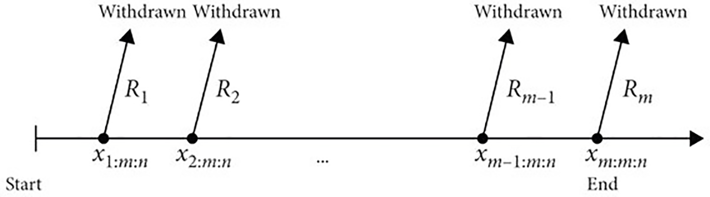
Figure 1: PTIIC scheme

Statistical modeling of lifetime data in engineering and medicine requires flexible distributions to capture complex behaviors like non-monotonic hazard rates and heavy-tailed distributions. Existing models, such as Weibull and Generalized Exponential, often fail to fit datasets with diverse shapes. EOEGE–E distribution offers unique advantages over existing models like Weibull and Generalized Exponential distributions. Its ability to model both monotonic and non-monotonic hazard rates (e.g., bathtub-shaped) makes it suitable for complex datasets in engineering (e.g., reliability analysis) and medicine (e.g., survival analysis). Unlike simpler models, the EOEGE–E captures heavy-tailed and skewed data, providing superior fit, as demonstrated in Section 6.

The remainder of the paper is structured as follows: Section 2 outlines the cumulative distribution function, density function, survival function, and hazard rate function of the extended odd exponential generalized exponential-exponential (EOEGE−E(Λ)) distribution, where Λ represents a vector of parameters. Additionally, graphical representations of the probability density function (pdf), cumulative distribution function (cdf), and hazard rate function of the EOEGE−E(Λ) distribution are presented. In Section 3, various statistical properties such as the quantile function, skewness, kurtosis, moments, and moment generating function are examined. The six estimation methods are studied in Section 4. In Section 5, Simulation is conducted to compare the performance of six proposed estimation methods. In Section 6, three complete real data are analysed for illustrating the usefulness of the proposed distribution. In Section 7, Simulation is conducted to compare the performance of two proposed estimation methods under PTIIC. Conclusion remarks is presented in Section 8.

2  The EOEGE-E Model

In this section, we develop a new class of odd generalized exponential-exponential model, known as Extended Odd Exponential Generalized Exponential distribution (EOEGE−E) with vector Λ=(α,β,λ,γ). The CDF of EOEGE − E is given as:

F(x;Λ)=(1−e−λ(eαxγγ−1))β,(4)

where x≥0 and Λ=(α,β,λ,γ)>0. The PDF, the SF and the HRF have the following forms

f(x;Λ)=αλβxγ−1eαxγγe−λ(eαxγγ−1)(1−e−λ(eαxγγ−1))β−1,(5)

where β is a shape parameter, λ>0, α and γ are scale parameters.

The survival function (SF) is given by

S(x;Λ)=1−(1−e−λ(eαxγγ−1))β.(6)

The hazard rate function (HRF) is given by

h(x;Λ)=βλαxγ−1eαxγγe−λ(eαxγγ−1)(1−e−λ(eαxγγ−1))β−11−(1−e−λ(eαxγγ−1))β.(7)

The graphical representations in Figs. 2 and 3 illustrate the remarkable flexibility and adaptability of the EOEGE–E distribution, driven by its parameters α,β,λ and γ. PDF plots demonstrate the ability of the distribution to exhibit symmetric, right- or left-skewed shapes depending on parameter values. For example, higher β values yield more symmetric densities profiles, suitable for balanced datasets, while lower γ values increase skewness, making the distribution ideal for modeling heavy-tailed engineering failure times. Survival function (SF) plots consistently show decreasing survival probabilities, a critical feature for reliability analysis in engineering applications. Furthermore, the hazard rate function (HRF) can exhibit increasing bathtub or bathtub shapes, such as with α=0.5,β=1.3, which is particularly valuable to model medical survival data with initial high-risk periods. These characteristics underscore the robustness of the EOEGE–E distribution, making it a powerful tool for statistical analysis in engineering, medicine, and other applied sciences.

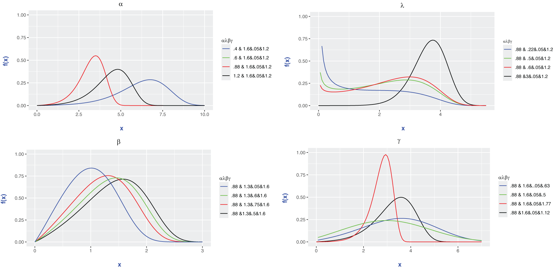
Figure 2: Shape and behaviour of pdf plots with several values of parameters α, β, λ and γ

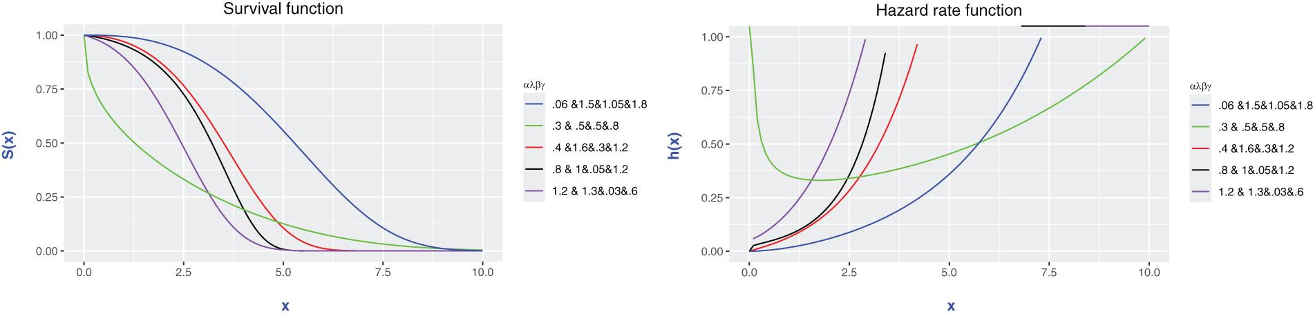
Figure 3: Survival function and Hazard rate function

3  Several Statistical Properties

In the beginning of this section, several useful expansions of the PDF and CDF of the new EOEGE − E distribution are shown below using a well-known generalized binomial and power series expansion. It is presented to justify the analytical divergence of some basic distribution features. The expansions of the generalized binomial and power series are as follows:

∑j=0∞(b−1j)(−1)jzj=(1−z)b−1,e−x=∑j=0∞(−1)jxjj!.(8)

The EOEGE − E distribution’s PDF and CDF are then displayed as follows:

f(x;Λ)=αβ∑j=0∞∑i=0∞∑k=0∞(jk)(β−jj)(1+j)iλj+1(−1)j+i+kj!xγ−1e−α(k−j−1)xγγ,(9)

F(x;Λ)=∑j=0∞(β−jj)(−1)je−λj(eαxγγ−1).(10)

3.1 Quantile Function

The quantile function of the EOEGE–E distribution is derived in Appendix A.

In particular, the Galton skewness coefficient and Moors kurtosis coefficient is applicable for calculating skewness and kurtosis as following

Sk=(x0.75−2x0.5+x0.25)(x0.75−x0.25),(11)

Kv=x0.875−x0.625+x0.375+x0.125x0.75−x0.25.(12)

Figs. 4–9 display the skewness and kurtosis plot for the EOEGE–E distribution with different parameter values. The EOEGE–E distribution is found to be symmetric, positively skewed, and slightly negatively skewed. It could also be mesokurtic, platykurtic, or leptokurtic.

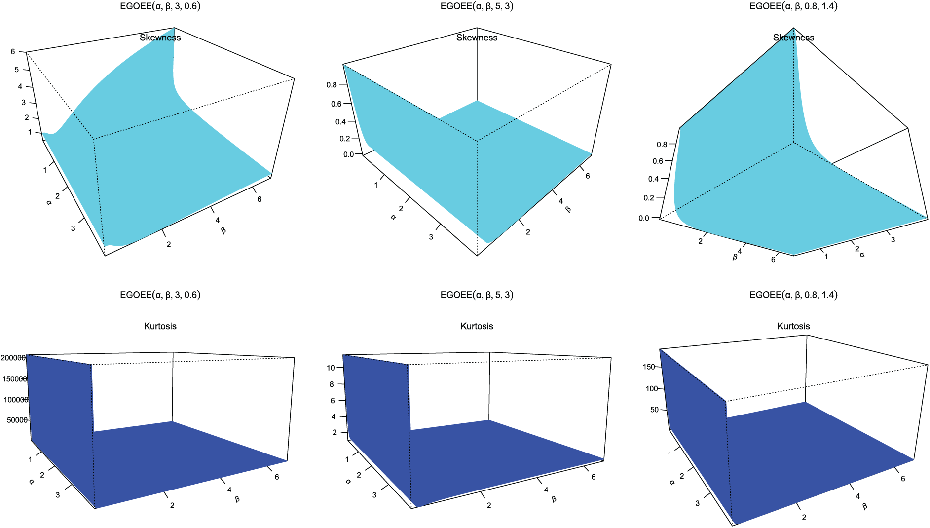
Figure 4: Skewness and kurtosis plots for EOEGE-E parameters α and β

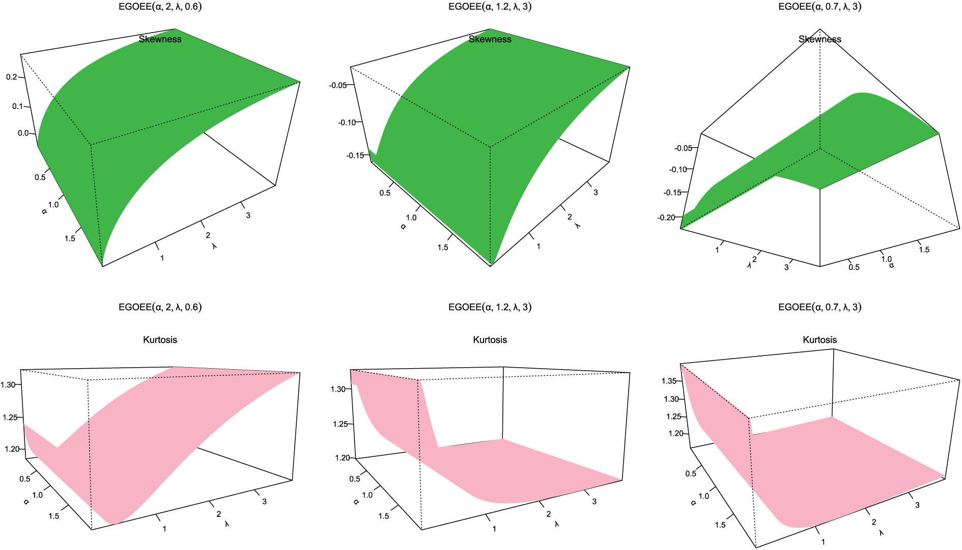
Figure 5: Skewness and kurtosis plots for EOEGE-E parameters α and λ

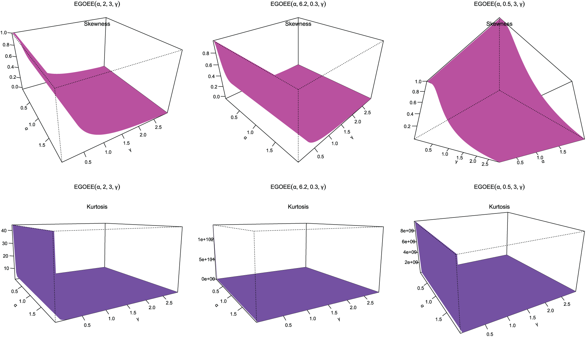
Figure 6: Skewness and kurtosis plots for EOEGE-E parameters α and γ

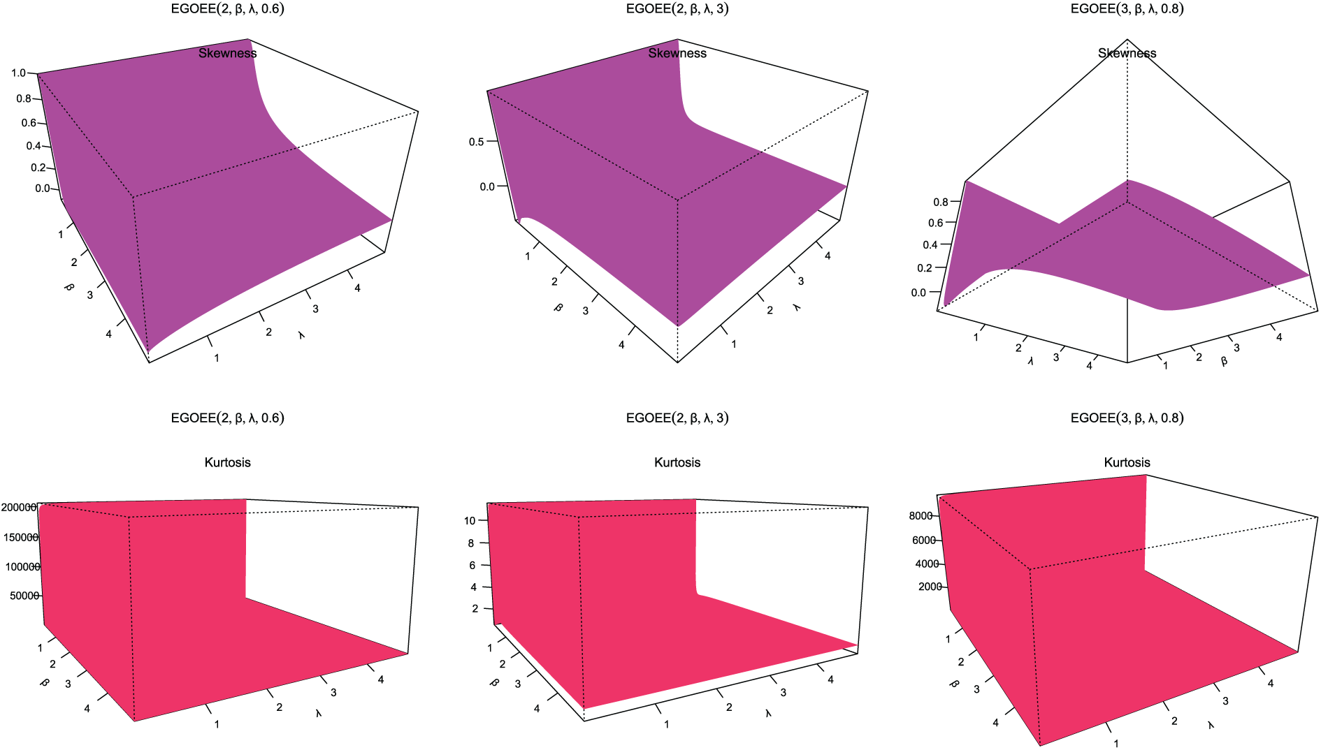
Figure 7: Skewness and kurtosis plots for EOEGE-E parameters β and λ

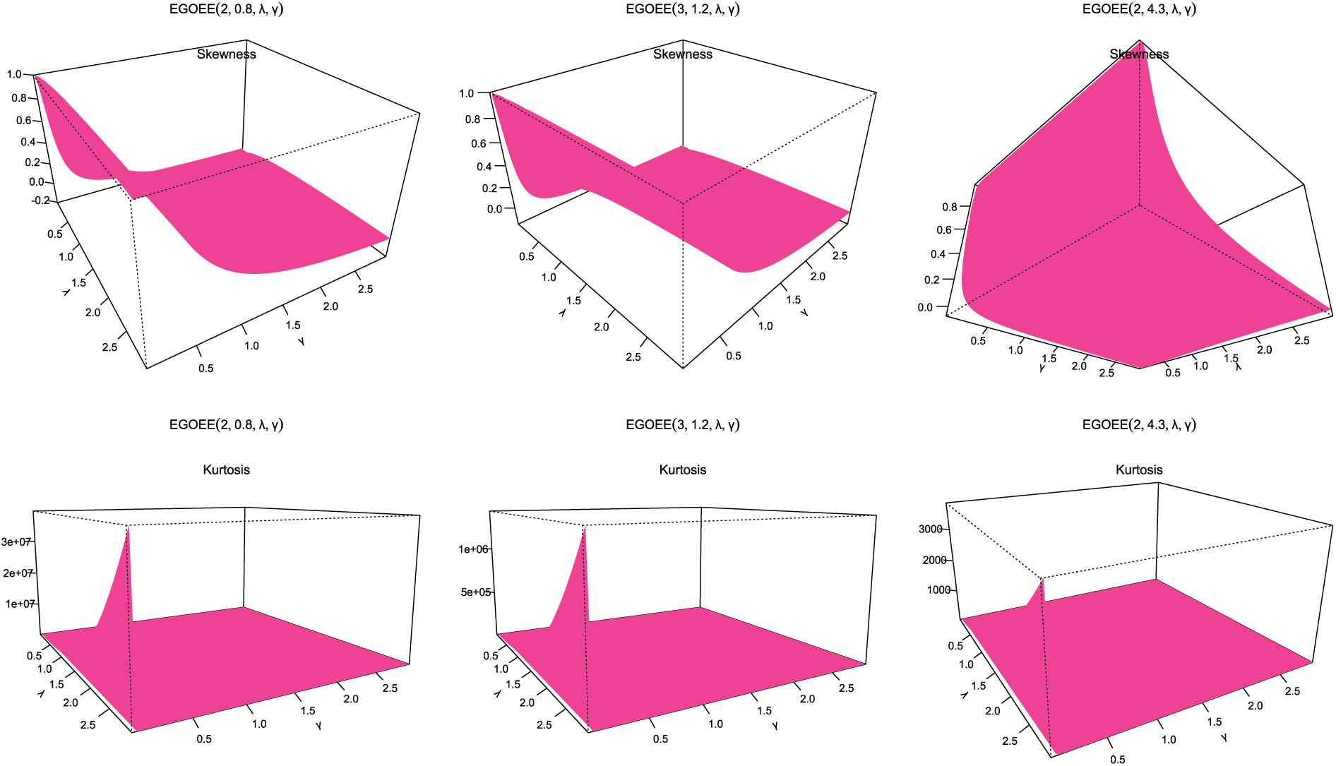
Figure 8: Skewness and kurtosis plots for EOEGE-E parameters λ and γ

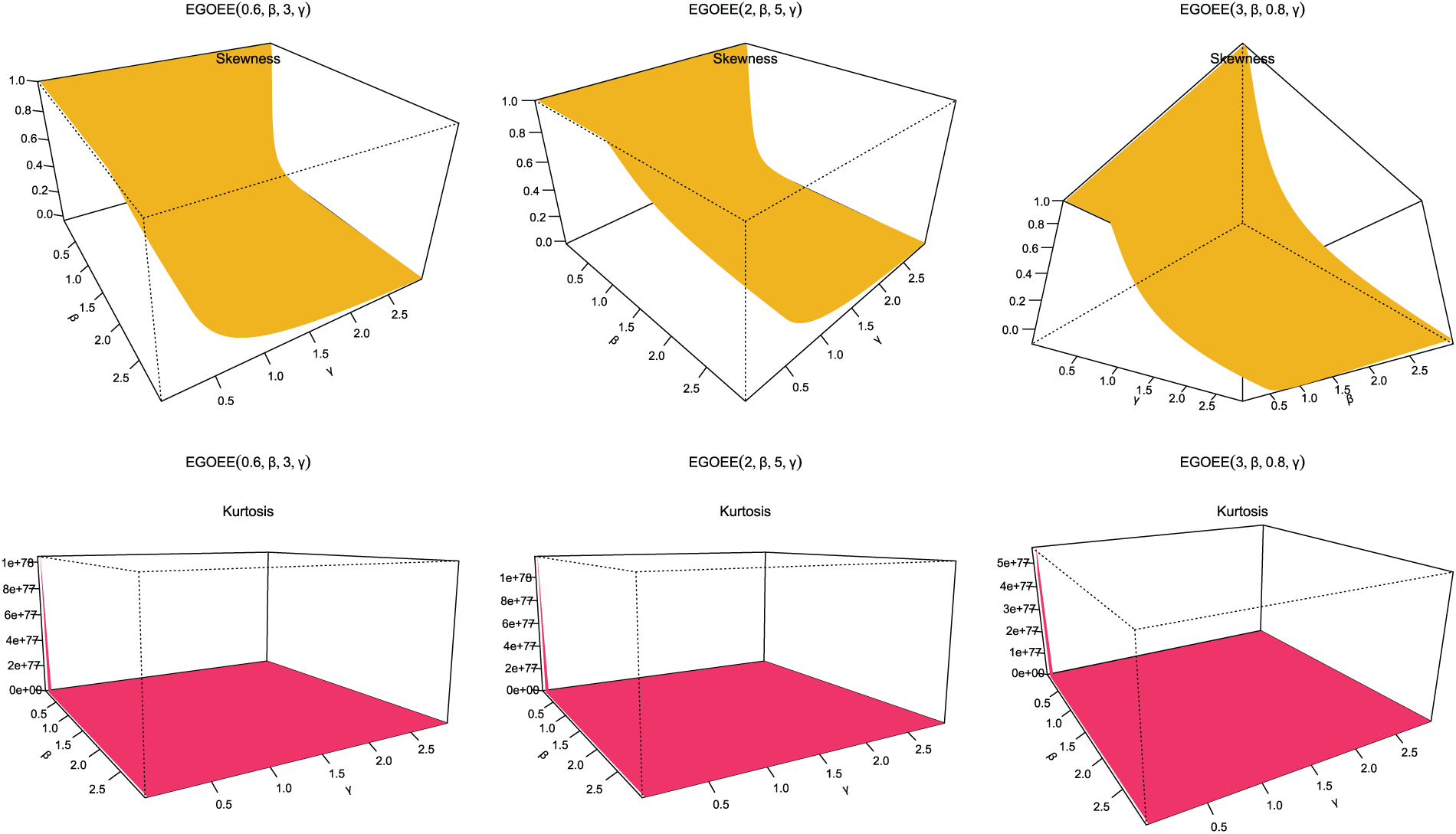
Figure 9: Skewness and kurtosis plots for EOEGE-E parameters β and γ

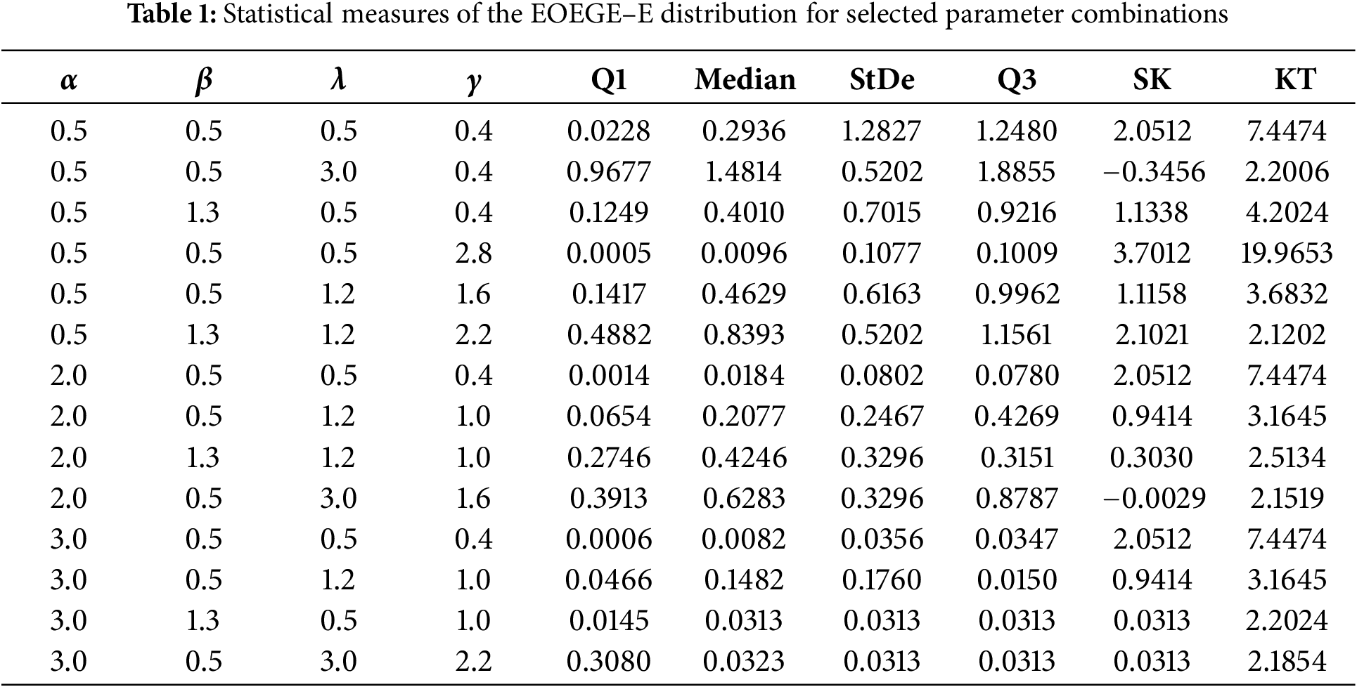
Table 1 displays key statistical measures for the EOEGE–E distribution across 14 parameter combinations with α=0.5,2,3 and varying β, λ, and γ. These measures include the first quartile (Q1), median, mean, standard deviation (StDe), third quartile (Q3), skewness (SK), and kurtosis (KT). The table highlights the distribution’s ability to model symmetric, skewed, or heavy-tailed data effectively. It shows a wide range of skewness (SK: −0.3456 to 3.7012) and kurtosis (KT: 2.1202 to 19.9653), making it adaptable to diverse datasets. For instance, a high γ (e.g., γ=2.8) results in strong positive skewness (SK = 3.7012), while higher γ values tend to reduce skewness and kurtosis, creating more symmetric distributions. Conversely, a high λ (e.g., λ=3) can lead to negative skewness (SK = −0.3456), and a lower λ increases variability, ideal for analyzing engineering failure times. Additionally, a higher α (e.g., α=3) paired with β=1.3 produces nearly symmetric data (SK = 0.0313). These properties demonstrate the EOEGE–E distribution’s versatility for engineering and medical data applications.

3.2 The r-th Moments

r-th moments of the EOEGE–E distribution are derived in Eq. (A1).

3.3 The Moment Generating Function

We derive the moment generating function using an infinite expansion of the EOEGE−E distribution, as follows: The moment generating functions of random variable Xr is provided by

MX(t)=E(etXr)=∫0∞etxrf(x)dx(13)

using series expansion etxr, we obtain

MX(t)=∑r=0∞trr!E(Xr).(14)

Substiuting from Eq. (5), we get The moment generating function MX(t) of random variable X∼EOEGE−E is

MX(t)=(−1)rγαβ(γ)rγΓ(1+rγ)∑r=0∞∑j=0∞∑i−0∞∑k=0∞tr(1α(k−j−1))r+γγ(jk)(β−1j)(1+j)iλj+1(−1)j+i+kr!j!,(15)

for any Λ=(α,β,λ,γ)>0.

3.4 Order Statistics

Consider n independent and identically distributed random variables, denoted as X1,…,Xn, following the EOEGE−E distribution. Let X(1)≤X(2)≤…≤X(n) represent the order statistic derived from these n variables. The probability density function (pdf) of the r-th order statistic, denoted as fr:n(x), is defined as follows:

fr:n(x)=Cr:nf(x)[F(x)]r−1[1−F(x)]n−r,r=1,2,…,n,(16)

where Cr:n=n!(r−1)!(n−r)!. Then

fr:n(x)=Cr:nf(x)∑j=0n−r(−1)j(n−rj)[F(x)]r+j−1

Substituting cdf and pdf given by Eqs. (4) and (5) in Eq. (16), respectively, then the rth order statistics of EOEGE−E distribution is

fr:n(x)=Cr:nf(x)∑j=0n−r(−1)j(r+j)(n−rj)f(x,α,(r+j)β,λ,γ),(17)

where f(x,α,(r+j)β,λ,γ) denotes the pdf of EOEGE−E distribution with parameters α,(r+j)β,λ and γ. So, the density function of EOEGE−E order statistics is a mixture of EOEGE−E densities.

4  Estimation Methods

In this context, six estimation methods are employed to estimate the parameters Λ=(α,β,γ) of the EOEGE–E distribution. These methods include maximum likelihood estimation (MLE), ordinary least squares estimation (OLSE), weighted least squares estimation (WLSE), maximum product spacing estimation (MPSE), Cramér-von Mises estimation (CVME), and Anderson-Darling estimation (ADE). The six estimation methods (MLE, OLS, WLS, MPS, CVM, AD) were chosen to balance computational efficiency and statistical robustness. Unlike simpler methods (e.g., method of moments), these approaches leverage the EOEGE–E’s likelihood structure, ensuring accurate parameter estimates for complex datasets. MLE and MPS are extended to censored data in Section 7, justified by their superior performance in simulation studies (Tables 2–5).

4.1 Maximum Likelihood Estimation (MLE)

Let X1,X2,…,Xn is a random sample of size n from new EOEGE−E, then the likelihood function L(Λ)=∏i=1nf(xi;Λ) is given by

L(Λ)=∏i=1n(αλβxiγ−1eαxiγγe−λ(eαxiγγ−1)(1−e−λ(eαxiγγ−1))β−1).

The function expressing the natural logarithm of the likelihood is provided as follows:

ℓ(Λ)=nln⁡(αβλ)+(γ−1)∑i=1nln⁡xi−∑i=1nλ(eαxiγγ−1)+λγ∑i=1nxiγ+(β−1)∑i=1nln⁡[1−eλ(eαxiγγ−1)].

Partial derivatives of previous equation for (α,β,λ,γ), respectively, yield

∂ℓ∂α=nα−λ∑i=1nxiγγeαxiγγ+(β−1)∑i=1nλxiγγeαxiγγ(eλ(eγxiγγ−1)−1))=0∂ℓ∂λ=nλ−∑i=1n(eαxiγγ−1)+(β−1)∑i=1n(eαxiγγ−1)(eλ(eαxiγγ−1)−1)=0∂ℓ∂β=nβ+∑i=1n[1−e−λ(eαxiγγ−1)]=0

∂ℓ∂γ=∑i=1nln⁡(xi)+αγ2∑i=1nxiγ−αγ∑i=1nxiγln⁡xi−λαγ2∑i=1nxiγ(1−γln⁡xi)eαxiγγ

+(β−1)αλγ2∑i=1n(xiγ(1−γln⁡xi)(eαxiγγ−1)(eλ(eαxiγγ−1)−1)=0

Estimators of maximum likelihood (MLEs) of the four above systems of non-linear equations can be found numerically for α,β,λ and γ equations, but there is no analytical solution for MLEs. As a result, iterative techniques such as the Newten-Raphsen type algorithm are an appropriate choice for supporting the simulation research of MLEs.

4.2 Ordinary Least Squares (OLS) and Weighted Least Squares (WLS)

Consider a random sample X(1),X(2),…,X(n) drawn from the EOEGE–E distribution with parameters Λ=(α,β,γ). The Ordinary Least Squares (OLS) and Weighted Least Squares (WLS) estimators for the parameters can be obtained by minimizing the following function with respect to the parameters:

S(Λ)=∑i=1nwi[(1−e−λ(eαx(i)γγ−1))β−in+1]2,

where wi=1 for OLSE and wi=(n+1)2(n+2)i(n+1−i) for WLSE. OLS and WLS estimators can be determined by solving the non linear equations

∂S∂α=2∑i=1nwiD1(x(i))[(1−e−λ(eαx(i)γγ−1))β−in+1],

∂S∂β=2∑i=1nwiD2(x(i))[(1−e−λeαx(i)γγ−1))β−in+1],

∂S∂λ=2∑i=1nwiD3(x(i))[(1−e−λ(eαx(i)γγ−1))β−in+1],

∂S∂γ=2∑i=1nwiD4(x(i))[(1−e−λ(eαx(i)γγ−1))β−in+1],

where

D1(x(i),Λ)=βλγx(i)γeαx(i)γγe−λ(eαx(i)γγ−1)(1−e−λ(eαx(i)γγ−1))β−1,(18)

D2(x(i),Λ)=(1−e−λ(eαx(i)γγ−1))βln⁡(1−e−λ(eαx(i)γγ−1)),(19)

D3(x(i),Λ)=β(1−e−λ(eαx(i)γγ−1))β−1eαx(i)γγe−λ(eαx(i)γγ−1)(20)

and

D4(x(i),Λ)=βλαγx(i)γeαx(i)γγe−λ(eαx(i)γγ−1)(1−e−λ(eαx(i)γγ−1))β−1(ln⁡(x(i))−γ−1).(21)

4.3 Maximum Product of Spacing (MPS)

Let X(1),X(2),…,X(n) be a random sample from EOEGE−E distribution with parameters Λ=(α,β,γ). The idea of MPSE is to maximize the following equation

P(Λ)=1n+1∑i=1n+1log⁡[(1−e−λ(eαx(i)γγ−1))β−(1−e−λ(eαx(i−1)γγ−1))β],

with respect to Λ. We can identify the MPS estimators by solving the following equations:

∂P∂α=1n+1∑i=1n+1[D1(x(i),Θ)−D1(x(i−1),Θ)(1−e−λ(eαx(i)γγ−1))β−(1−e−λ(eαx(i−1)γγ−1))β],

∂P∂β=1n+1∑i=1n+1[D2(x(i),Θ)−D2(x(i−1),Θ)(1−e−λ(eαx(i)γγ−1))β−(1−e−λ(eαx(i−1)γγ−1))β],

∂P∂λ=1n+1∑i=1n+[D3(x(i),Θ)−D3(x(i−1),Θ)(1−e−λ(eαx(i)γγ−1))β−(1−e−λ(eαx(i−1)γγ−1))β],

∂P∂γ=1n+1∑i=1n+1[D4(x(i),Θ)−D4(x(i−1),Θ)(1−e−λ(eαx(i)γγ−1))β−(1−e−λ(eαx(i−1)γγ−1))β],

and D1(x(i),Λ),D2(x(i),Λ),D3(x(i),Λ) and D4(x(i),Λ) are defined in Eqs. (18)–(21).

4.4 Cramer Von-Mises (CVM)

Consider a random sample X(1),X(2),…,X(n) drawn from the EOEGE–E distribution. The CVM estimators can be obtained by minimizing the following equation

C(Λ)=112n+∑i=1n[(1−e−λ(eαx(i)γγ−1))β−2i−12n]2,

with respect to Λ. In addition, We can identify the CVM estimators by solving the following equations:

∂C∂α=2∑i=1nD1(x(i),Θ)[(1−e−λ(eαx(i)γγ−1))β−2i−12n],

∂C∂β=2∑i=1nD2(x(i),Θ)[(1−e−λ(eαx(i)γγ−1))β−2i−12n],

∂C∂λ=2∑i=1nD3(x(i),Θ)[(1−e−λ(eαx(i)γγ−1))β−2i−12n],

∂C∂γ=2∑i=1nD4(x(i),Θ)[(1−e−λ(eαx(i)γγ−1))β−2i−12n],

where D1(x(i),Λ),D2(x(i),Λ),D3(x(i),Λ) and D4(x(i),Λ) are defined in Eqs. (18)–(21).

4.5 Anderson-Darling (AD)

Consider a random samples X(1),X(2),…,X(n) drawn from the EOEGE–E distribution. The AD estimators can be obtained by minimizing the following equation

A(Λ)=−1n−n∑i=1n(2i−1)[log⁡(1−e−λ(eαx(i)γγ−1))β+log⁡(1−e−λ(eαx(n+1−i)γγ−1))β],

with respect to Λ. In addition, We can identify the AD estimators by solving the following equations:

∂A∂α=−n∑i=1n(2i−1)[D1(x(i),Θ)(1−e−λ(eαx(i)γγ−1))β+D1(x(n+1−i),Θ)(1−e−λ(eαx(n+1−i)γγ−1))β],

∂A∂β=−n∑i=1n(2i−1)[D2(x(i),Θ)(1−e−λ(eαx(i)γγ−1))β+D2(x(n+1−i),Θ)(1−e−λ(eαx(n+1−i)γγ−1))β],

∂A∂λ=−n∑i=1n(2i−1)[D3(x(i),Θ)(1−e−λ(eαx(i)γγ−1))β+D3(x(n+1−i),Θ)(1−e−λ(eαx(n+1−i)γγ−1))β],

∂A∂γ=−n∑i=1n(2i−1)[D4(x(i),Θ)(1−e−λ(eαx(i)γγ−1))β+D4(x(n+1−i)(1−e−λ(eαx(n+1−i)γγ−1))β],

where D1(x(i),Λ),D2(x(i),Λ),D3(x(i),Λ) and D4(x(i),Λ) are defined in Eqs. (18)–(21).

The non-linear equations derived from the log-likelihood are solved using the Newton-Raphson method. For parameters Λ=(α,β,λ,γ), the algorithm iterates as

Λk+1=Λk−H−1(Λk)∇ℓ(Λk),

where ∇ℓ is the gradient and H is the Hessian of the log-likelihood. Initial guesses are set based on moment estimates, and convergence is achieved when |Λk+1−Λk|<10−6. Computations were performed in R using the ‘optim’ function, ensuring robust solutions.

5  Simulation Study

A Monto Carlo (MC) simulation study is carried out to explore and assess the behavior of MLEs of EOEGE–E model via R program. We consider 1000 MC-replicates under different sample sizes n = 50, 100, 200, and 300.

The samples have been drawn for different cases as follows:

•   Case 1: α=2.5,β=1.5,λ=0.8,γ=0.5.

•   Case 2: α=0.75,β=1.5,λ=0.8,γ=0.5.

•   Case 3: α=0.75,β=0.5,λ=1.6,γ=2.

•   Case 4: α=0.75,β=0.5,λ=0.8,γ=0.5.

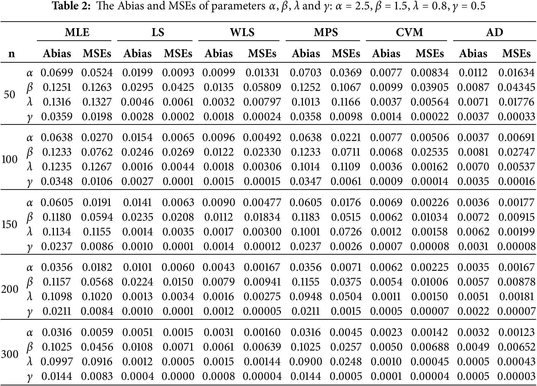
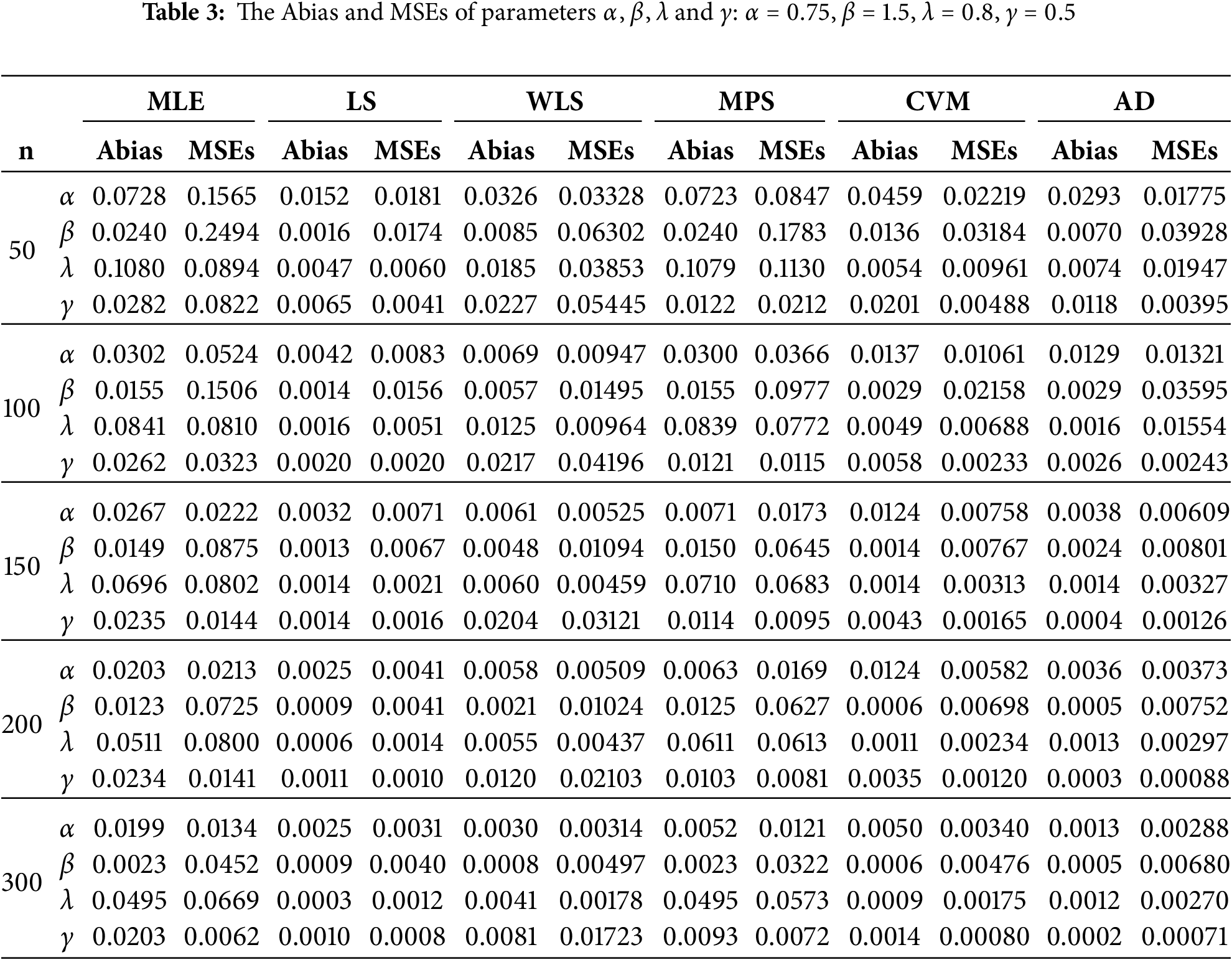
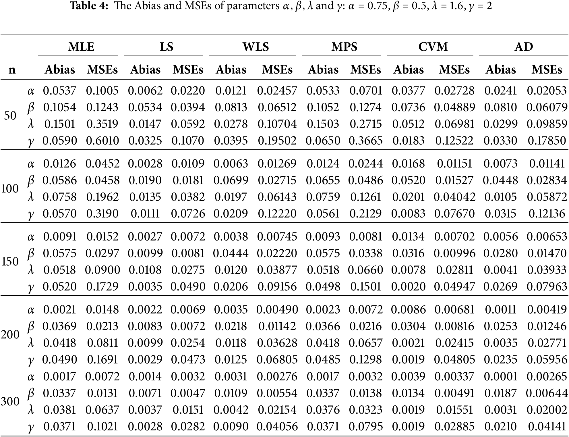
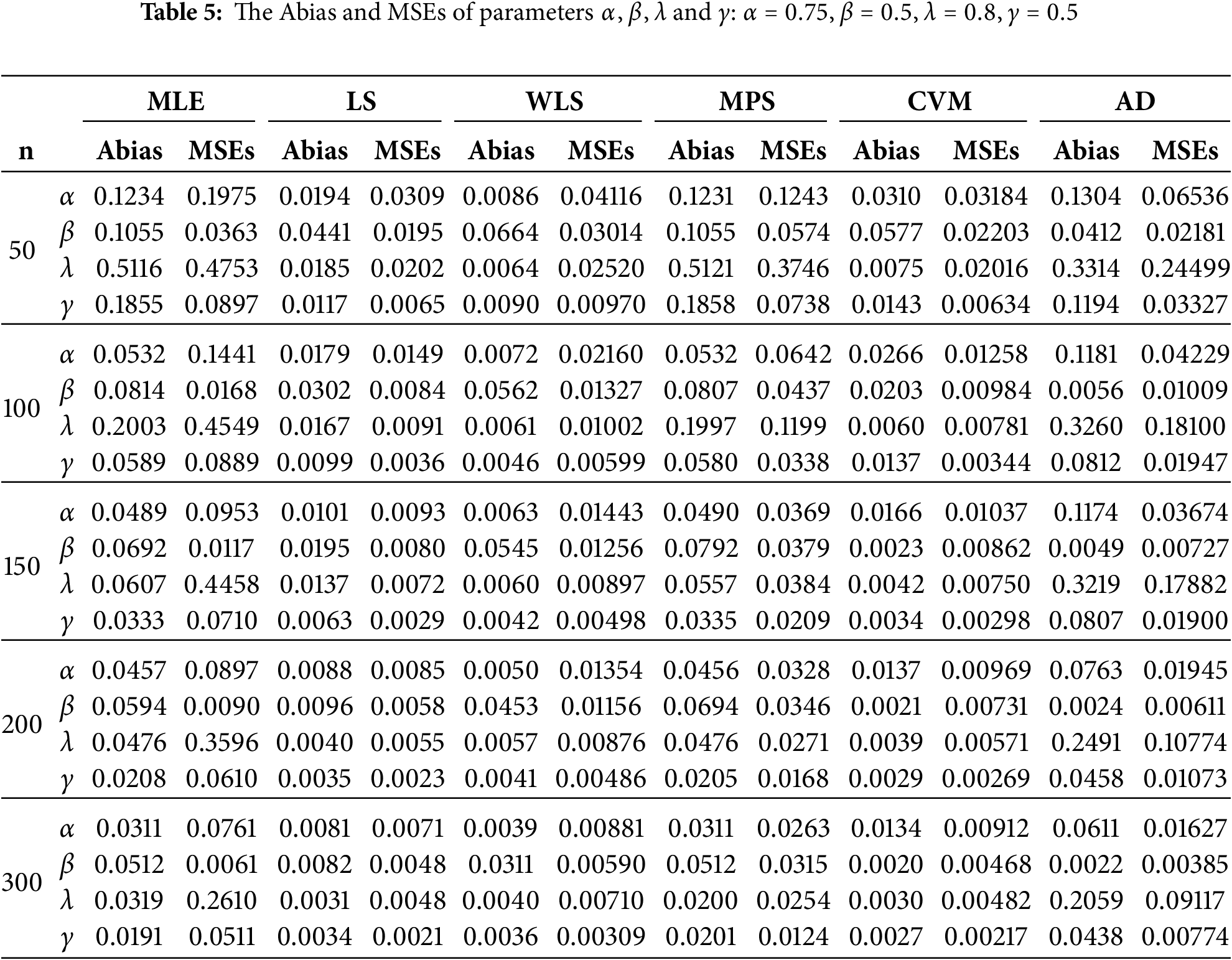
For each sample size, we compute the MLE, LS, WLS, MPS, CVM, and AD with different measures as Absolute Biases (ABias) and mean square error (MSEs) for all estimates methods. All simulation experiments were conducted using the R software. The likelihood function was optimized using the optim function with the Nelder-Mead algorithm. These methods are well-established in statistical analysis and contribute to the reliability and accuracy of the obtained results. The results obtained after performing the MC simulation and ABias and MSEs are presented in Tables 2–5. The following conclusions can be made based on the data presented in Tables 2–5:

•   With larger sample sizes (n), there is a decrease in both the Abias and MSEs of all estimators, indicating better precision in estimating model parameters, indicating consistency behaviour.

•   The methods yielding the least biased parameters across different sample sizes (n) are CVM, and WLS methods.

•   Across all n’s, the Abias of the estimators tends to approach zero, indicating unbiased estimation.

The simulation results indicate that the MPSE often provides more accurate estimates in terms of both bias and mean squared error, particularly for small and moderate sample sizes. This can be attributed to the spacing-based nature of the MPSE, which tends to perform better under skewed or heavy-tailed distributions—features that characterize the proposed EOEGE–E distribution. While the MLE is asymptotically efficient, its performance may deteriorate when the likelihood function is complex or when the sample size is small. The OLSE and WLSE exhibit sensitivity to heteroscedasticity in the transformed data, leading to less stable estimates. The CVME and ADE methods show balanced performance, with ADE particularly effective in the presence of extreme values due to its emphasis on tail behavior. These findings suggest that the choice of estimation method should be informed by the sample size and the underlying characteristics of the data.

6  Real Data Analysis

Three real data sets applications to illustrate the importance and flexibility of the family are presented.

Data set 1. Failure time of 69 components. Badar and Priest [20] discussed the data set of sample size 69 observed failure times, the dataset is represented the data measured in GPA (Gigapascals), for single carbon fibers and impregnated 1000 carbon fiber The data set values are: 0.562, 0.564, 0.729, 1.216, 1.474, 1.632, 1.816, 2.020, 2.317, 1.247, 1.490, 1.676, 1.824, 2.023, 2.334, 1.256, 1.503, 1.684, 1.836, 2.050, 2.340, 0.802, 1.271, 1.520, 1.685, 1.879, 2.059, 2.346, 0.950, 1.277, 1.522, 1.728, 1.883, 2.068, 2.378, 1.053, 1.305, 1.524, 1.740, 1.892, 2.071, 2.483, 1.111, 1.348, 1.551, 1.764, 1.934, 2.130, 2.835, 1.115, 1.313, 1.551, 1.761, 1.898, 2.098, 2.683, 1.194, 1.390, 1.609, 1.785, 1.947, 2.204, 2.835, 1.208, 1.429, 1.632, 1.804, 1.976, 2.262. For data set 1, the MLEs of the parameters, Kolmogorov-Smirnov (KS) and the p value are calculated and displayed in Table 6 demonstrated the commonly used well-known model selection information criterion, namely, AIC, CAIC (Consistent Akaike Information Criterion), BIC, and HQIC with important measures including Anderson-Darling (AD) and Cramer-von Mises (CVM). The EOEGE–E distribution is compared with other competitive models as: Alpha power exponential (APEx) [21], The exponentiated generalized alpha power family (EGAPEx) [22], Half logistic exponentiated inverse Rayleigh distribution (HLEIRD) [23], the exponentiated generalized exponential (EGEx) [24], alpha power generalized exponential (APGEx) [25] and exponential (Ex) distributions. Fig. 10 includes six diagnostic plots (A–F) assessing the EOEGE–E distribution’s fit to the 69 failure times in Dataset I.

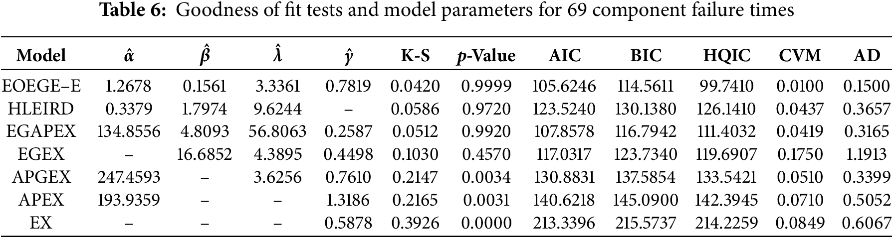
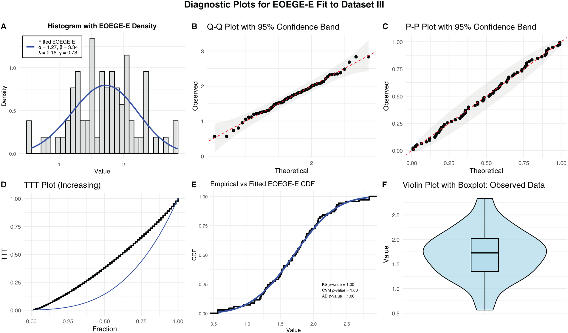
Figure 10: Diagnostic plots for EOEGE-E Fit to dataset I

The EOEGE–E distribution provides an exceptional fit to Dataset I, numerically, Table 6 shows EOEGE–E’s lowest Kolmogorov-Smirnov (K-S) statistic (0.0420), highest p-value (0.9999), and lowest Akaike Information Criterion (AIC, 105.6246), Bayesian Information Criterion (BIC, 114.5611), Hannan-Quinn Information Criterion (HQIC, 99.7410), Cramér-von Mises (CVM, 0.0100), and Anderson-Darling (AD, 0.1568) values, outperforming HLEIRD, EGAPEX, EGEX, APGEX, APEX, and EX. Visually, Fig. 10’s diagnostic plots confirm this:

•   The histogram and violin plots (A, F) show EOEGE–E capturing the right-skewed, heavy-tailed distribution.

•   Q-Q and P-P plots (B, C) validate quantile and probability alignment within 95% confidence bands.

•   The Total Time on Test (TTT) plot (D) confirms an increasing hazard rate, which EOEGE–E models accurately.

•   The cumulative distribution function (CDF) plot (E) shows near-perfect overlap with the empirical CDF.

Dataset I’s right-skewed failure times and increasing hazard rate, indicative of carbon fiber fatigue under stress, are ideally suited to EOEGE–E’s four-parameter flexibility. This makes EOEGE–E a powerful tool for reliability engineering, enabling accurate failure predictions and material design optimization. Competing models, especially EX, fail to capture these characteristics, highlighting EOEGE–E’s superiority.

Data set 2. Service times of 50 aircraft windshields. The second data presents the contains information on the “service times” of 50 aircraft windshields. Murthy et al.’s study [24] contains this information. Data are as follows: 1.0030, 1.436, 0.1400, 0.2800, 1.7940, 2.819, 2.592, 0.3130, 0.0460, 1.9150, 2.820, 0.3890, 1.9200, 2.878, 3.1020, 0.9520, 2.0650, 3.3040, 0.9960, 2.1170, 3.483, 1.0030, 2.1370, 3.500, 0.487, 1.9630, 2.950, 0.6220, 1.978, 3.0030, 0.9000, 2.0530, 1.0100, 2.141, 3.6220, 1.492, 2.600, 0.150, 1.580, 2.163, 3.6650, 1.092, 2.183, 3.6950, 1.1520, 2.2400, 4.015, 2.670, 0.248, 1.7190. Table 7 defines the parameter estimates, their standard errors (SE), are enclosed in bracket, Anderson-Darling (AD), Cram’er-von Mises (CVM), and Kolmogrov-Smirnov (K-S) tests and p values. The EOEGE–E distribution is compared with the well-known models in publications Al-Essa et al. [26], Chesneau and Yousof [27], Cordeiro et al. [28], Lemonte et al. [29] and Yousof et al. [30].

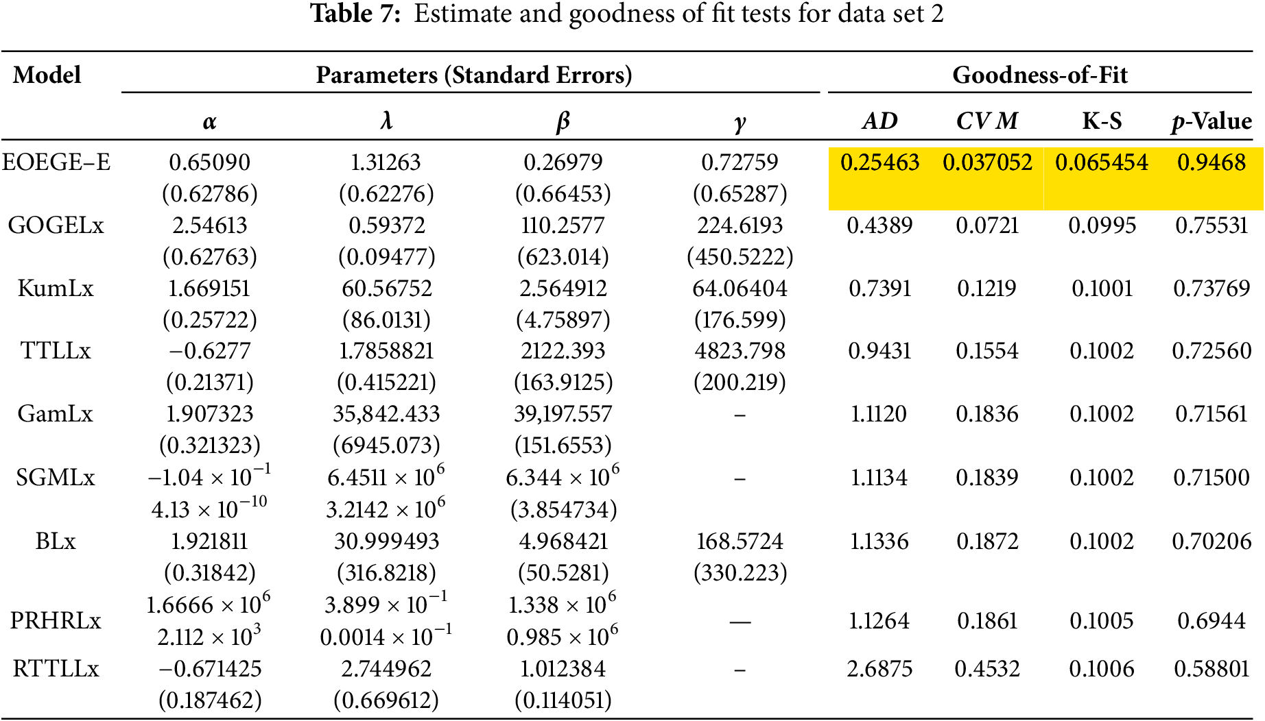
Fig. 11 and Table 7 demonstrate that the EOEGE–E distribution provides an excellent fit to Dataset II (service times of 50 aircraft windshields). Numerically, Table 7 shows EOEGE–E’s lowest Anderson-Darling (AD, 0.25463), Cramér-von Mises (CVM, 0.037052), and Kolmogorov-Smirnov (K-S, 0.065454) statistics, and highest p-value (0.9468), outperforming GOGELx, KumLx, TTLLx, GamLx, SGMLx, BLx, PRHRLx (Proportional Reversed Hazard Rate Lomax), and RTTLLx. Visually, Fig. 11’s diagnostic plots confirm this:

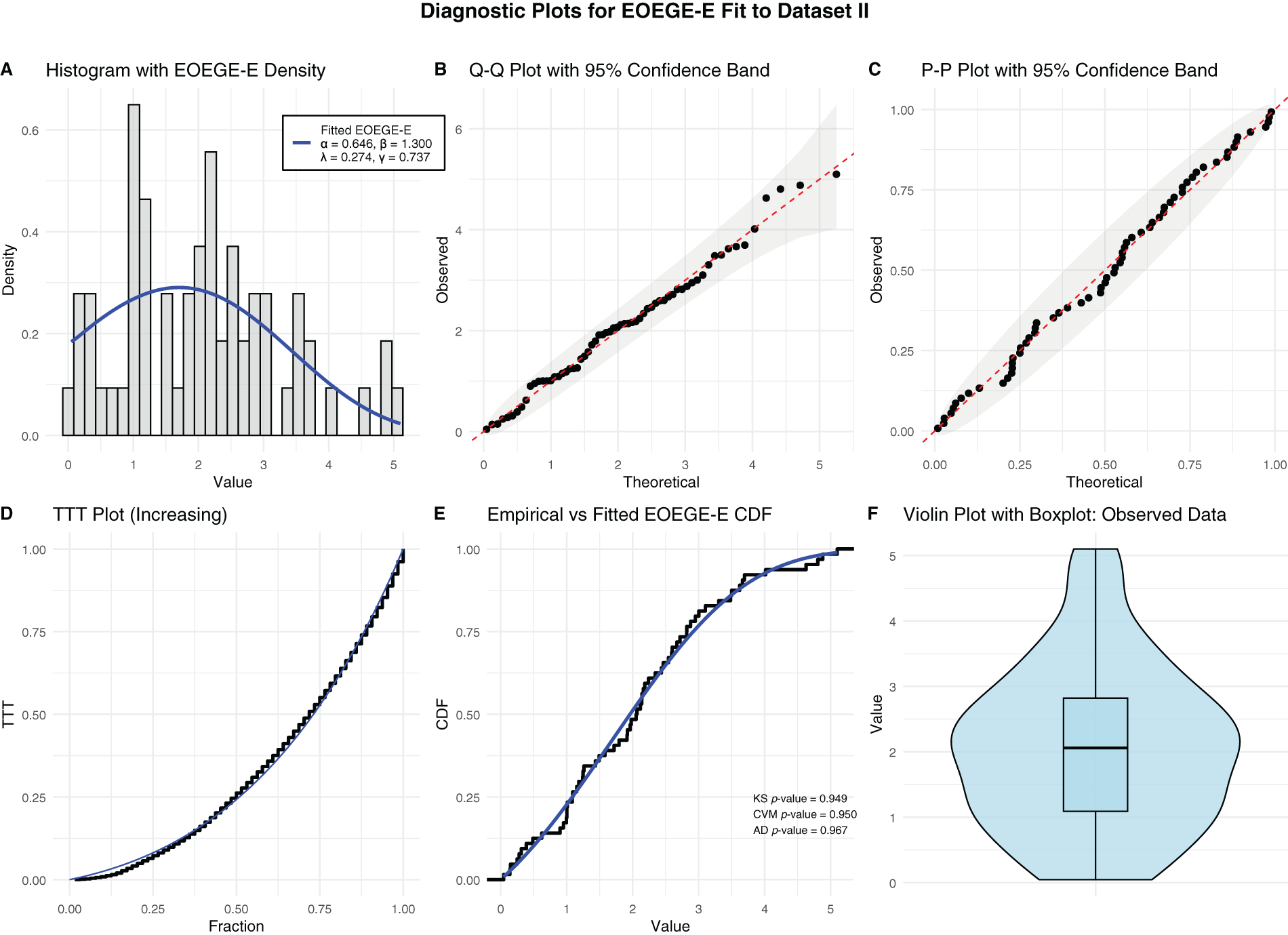
Figure 11: Diagnostic plots for EOEGE–E fit to dataset II

•   The histogram and violin plots (A, F) show EOEGE–E capturing the slightly left-skewed, long-tailed distribution.

•   Q-Q and P-P plots (B, C) validate quantile and probability alignment within 95% confidence bands.

•   The Total Time on Test (TTT) plot (D) confirms an increasing hazard rate, accurately modeled by EOEGE–E.

•   The cumulative distribution function (CDF) plot (E) shows near-perfect overlap with the empirical CDF.

Compared to Dataset I (right-skewed carbon fiber failure times), Dataset II’s different skewness and smaller sample size result in a slightly less precise fit, but EOEGE–E’s four-parameter flexibility ensures superior performance in both cases. This makes EOEGE–E a powerful tool for reliability engineering.

Data set 3. Blood cancer data set. The life time (in years) of a 40 blood cancer (leukemia) patients from one of Ministry of health hospitals in Saudi Arabia. This actual data are as follows: ‘0.315, 0.496, 0.616, 1.145, 1.208, 1.263, 1.414, 2.025, 2.036, 2.162, 2.211, 2.370, 2.532, 2.693, 2.805, 2.910, 2.912, 3.192, 3.263, 3.348, 3.348, 3.427, 3.499, 3.534, 3.767, 3.751, 3.858, 3.986, 4.049, 4.244, 4.323, 4.381, 4.392, 4.397, 4.647, 4.753, 4.929, 4.973, 5.074, 5.381’. For data set 3, the MLEs of the parameters, the commonly used wellknown model selection information criterion, namely, AIC and BIC with important measures including Anderson–Darling (AD), Cram’er–von Mises (CVM), and Kolmogrov–Smirnov (K–S) test and p value are computed and displayed in Table 8. The EOEGE–E distribution is compared with other some competitive models, including the exponentiated generalized Weibull Rayleigh distribution (EGWR) (Alsulami, 2025) [31], gamma log-logistic Weibull (GmLLW) (Foya et al., 2017) [32], Burr III Extended Exponentiated Weibull Distribution (BIIIEEW) (Hussian et al., 2023) [33], generalized odd beta prime Weibull (GOBPW) (Suleiman et al., 2022) [34], gamma generalized modified Weibull (GmGMoW) (Oluyede et al., 2015) [35] and beta modified Weibull (BMoW) (Silva et al., 2010) [36].

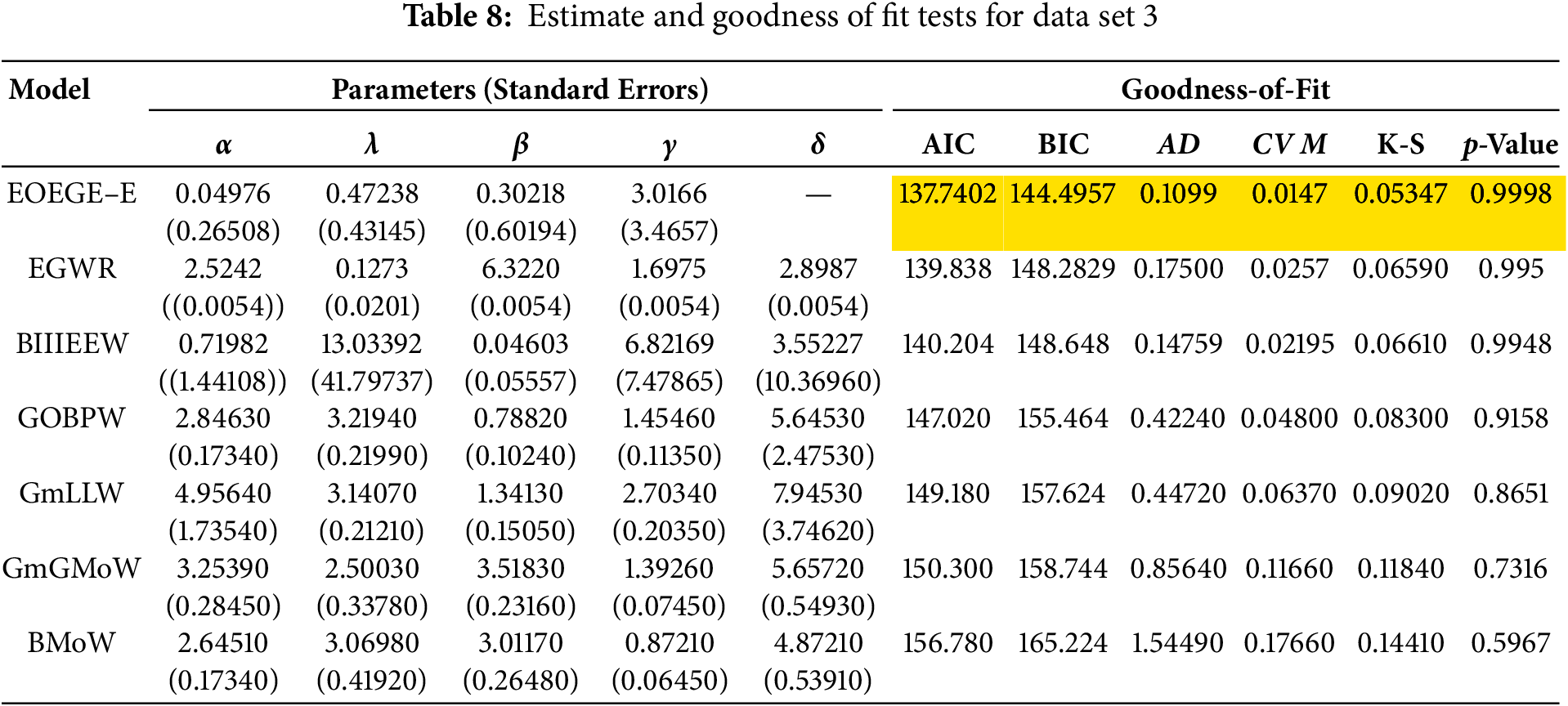
Table 8 demonstrates that the EOEGE–E distribution provides an exceptional fit to Dataset 3 and shows EOEGE–E’s lowest Akaike Information Criterion (AIC, 137.7402), Bayesian Information Criterion (BIC, 144.4957), Anderson-Darling (AD, 0.1099), Cramér-von Mises (CVM, 0.0147), and Kolmogorov-Smirnov (K-S, 0.05347) statistics, and highest p-value (0.9998), outperforming EGWR, BIIIEEW, GOBPW, GmLLW, GmGMoW, and BMoW. Accorging Fig. 12, EOEGE–E is expected to capture the left-skewed distribution (mean = 3.0859 < median = 3.3055) and likely increasing hazard rate, similar to Datasets 1 and 2, with:

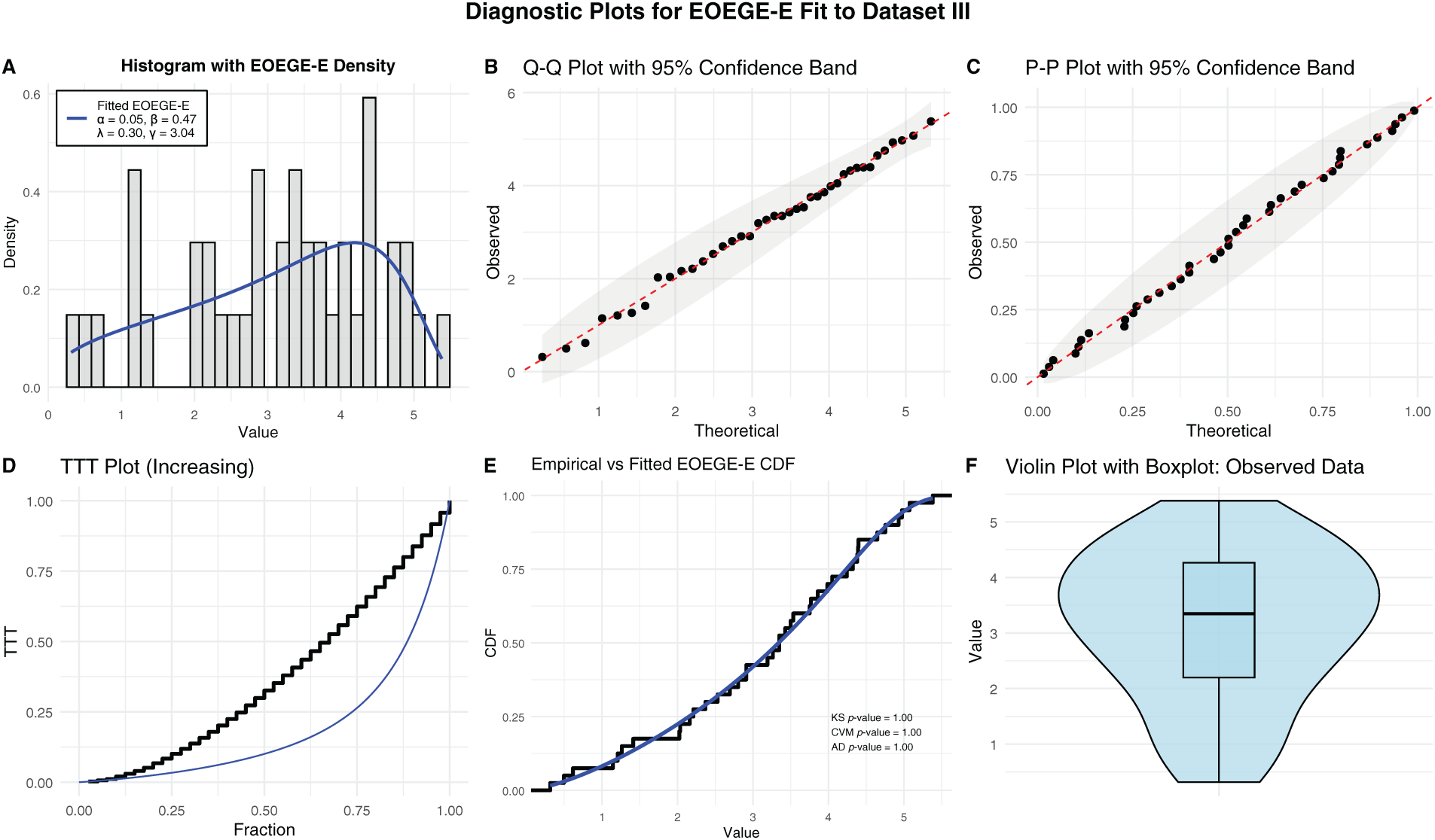
Figure 12: Diagnostic plots for EOEGE–E fit to dataset III

•   Histogram and violin plots showing alignment with the left-skewed, moderate-tailed distribution.

•   Q-Q and P-P plots validating quantile and probability alignment within 95% confidence bands.

•   A Total Time on Test (TTT) plot confirming an increasing hazard rate, reflecting disease progression.

•   A cumulative distribution function (CDF) plot showing near-perfect overlap with the empirical CDF.

Compared to Dataset 1 (right-skewed carbon fiber failure times, K-S = 0.0420, p-value = 0.9999) and Dataset 2 (slightly left-skewed windshield service times, K-S = 0.065454, p-value = 0.9468), Dataset 3’s fit is comparable to Dataset 1’s and superior to Dataset 2’s, despite the smaller sample size (n = 40 vs. 69 and 50). EOEGE–E’s four-parameter flexibility ensures robust modeling of diverse distributions and increasing hazard rates across material durability (Dataset 1), aviation maintenance (Dataset 2), and medical survival (Dataset 3). This makes EOEGE–E a powerful tool for reliability and survival analysis, enabling accurate prognosis prediction in healthcare and failure modeling in engineering.

Data set 4. Lifetime Data of Electronic Components The lifetimes of twenty electronic components, as reported by Murthy (2004, p. 100), are given in appropriate units as follows: 0.03, 0.12, 0.22, 0.35, 0.73, 0.79, 1.25, 1.41, 1.52, 1.79, 1.80, 1.94, 2.38, 2.40, 2.87, 2.99, 3.14, 3.17, 4.72, 5.09. These data represent the durations until failure for each component. For data set 4, the MLEs of the parameters, the commonly used wellknown model measures including Anderson–Darling (AD), Cram’er–von Mises (CVM), and Kolmogrov–Smirnov (K–S) test and p value are computed and displayed in Table 9. The EOEGE–E distribution is compared with other some competitive the extended odd weibull Lindley (ExOW-Li) (Alizadeh et al., 2018) [37], the new odd log-logistic (NOLL-L) model (Alizadeh et al., 2019) [38], the Topp-Leone Lindley distribution (TL-Li) (Al-Shomarni et al., 2016) [39], Odd log-logistic Lindley (OLL-Li) model (Ozel et al, 2017) [40], the Modefied half logistic (MHL) model (Mohammad, 2021) [41] and the Weighted Exponentiated class of Distributions (WExp-G) (Shaheed, 2025) [42].

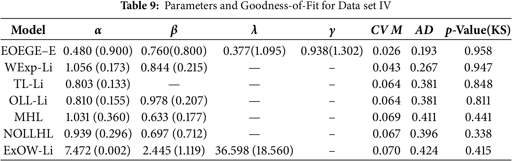
The Dataset IV lifetimes, with their right-skewed distribution, are best modeled by the EOEGE–E distribution, which achieves the lowest CVM (0.026), AD (0.193), and highest KS p-value (0.958). The EOEGE–E model’s fit is validated through six diagnostic plots in Fig. 13, which confirm its ability to capture Dataset IV’s characteristics:

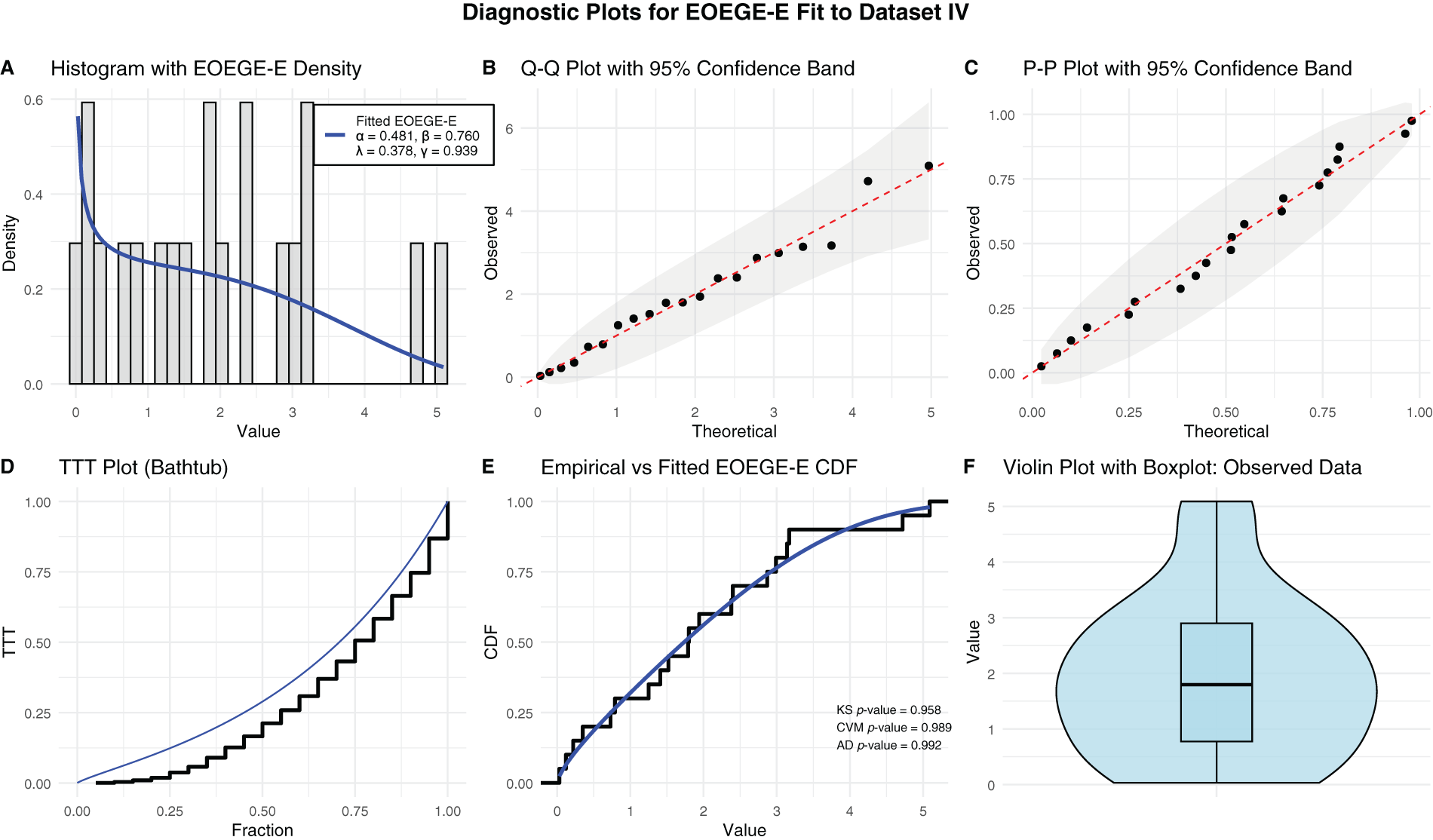
Figure 13: Diagnostic plots for EOEGE–E fit to dataset IV

•   Histogram and violin plots show alignment with the right-skewed, moderate-tailed distribution, capturing early failures and longer lifetimes effectively.

•   Q-Q and P-P plots validate quantile and probability alignment, with most points within 95% confidence bands, indicating minimal deviation from the observed data.

•   A Total Time on Test (TTT) plot confirms a bathtub-shaped hazard rate, reflecting electronic components’ early burn-in failures, stable operational period, and late wear-out, which EOEGE–E models accurately.

•   A cumulative distribution function (CDF) plot shows near-perfect overlap with the empirical CDF, consistent with the KS p-value of 0.958.

7  Progressive Type-II Censored Sample

The progressive type-II censoring scheme is commonly described as follows: Initially, n independent and identical units are subjected to a lifetime experiment. When the first failure occurs at time x(1), a random selection of r1 units is removed from the remaining n−1 surviving units. Subsequently, when the second failure occurs at time x(2), r2 units are randomly removed from the n−r1−2 surviving units. This process continues until the m-th failure is observed at time x(m), at which point the remaining rm=n−m−∑i=1m−1ri units are removed from the test. The censoring scheme, denoted as R=(R1,R2,…,Rm), is referred to as the progressive type-II censoring scheme. In progressive type-II right censoring, the censoring scheme R is predetermined before the experiment begins. Notably, type-II censoring is a special case of progressive type-II censoring, where the scheme is R=(0,0,…,n−m) (see [43]). Let X1:m:n,X2:m:n,…,Xm:m:n;1≤m≤n be a progressively type-II censored sample observed from a lifetime test involving n units and r1,r2,…,rm being the censoring scheme. The joint PDF of a progressively type-II censored sample is given by

f(x1:m:n,x2:m:n,…,xm:m:n)=C∏i=1mf (xi:m:n)[1−F(xi:m:n)]ri,(22)

where C may be a constant defined as

C=n (n−r1−1)⋯(n−∑i=1m−1(ri+1)). For more details, see [15–17,43].

We discussed the MLE and MPS for parameter estimator of the EOEGE-E distribution based on progressive type-II censored sample. Let X1:m:n,X2:m:n,…,Xm:m:n, 1≤m≤n be a progressively type-II censored sample observed from a life test involving n units taken from a population with PDF f(x) and CDF F(x) given in Eqs. (4) and (5), with the censoring scheme (R1,R2,…,Rm).

7.1 Maximum-Likelihood Estimation

From Eq. (22) the likelihood function of is then given by

L(Λ∣x¯)=αnrλnrβnre∑i=1nrαxi:m:nγγe−λ∑i=1nr(eαxi:m:nγγ−1)∏i=1nrxi:m:nγ−1(1−e−λ(eαxi:m:nγγ−1))β−1(1−(1−e−λ(eαxi:m:nγγ−1))β)Ri,

where x=x1:m:n,x2:m:n,…,xm:m:n.

The corresponding log-likelihood function for the parameters θ is

ℓ=log⁡L(Λ∣x¯)=nr(log⁡α+log⁡λ+log⁡β)+∑i=1nrαxi:m:nγγ−λ∑i=1nr(eαxi:m:nγγ−1)+(γ−1)∑i=1nrlog⁡xi:m:n+(β−1)∑i=1nrlog⁡(1−e−λ(eαxi:m:nγγ−1))+∑i=1nrRilog⁡(1−(1−e−λ(eαxi:m:nγγ−1))β).(23)

Since, derivatives of Eq. (23) for parameters does not has closed-form solution, the MLEs of α,β,λ and γ are obtained by maximizing the log-likelihood function given in Eq. (23). This results in a non-linear optimization problem, for which explicit solutions are generally not available. Consequently, numerical methods are employed to find the MLEs. The Newton–Raphson iteration method is employed to get the estimates.

To solve the system of nonlinear likelihood equations for the parameters α, β, λ, and γ, we employ the Newton-Raphson iterative method. This algorithm updates parameter estimates based on the following rule:

θ(k+1)=θ(k)−[∂2ℓ(θ)∂θ2]−1[∂ℓ(θ)∂θ],

where θ(k) denotes the estimate vector at the k-th iteration, and ℓ(θ) is the log-likelihood function. The iterations continue until convergence is achieved based on a predefined tolerance level (e.g., 10−6). The partial derivatives (gradient) and second derivatives (Hessian matrix) are computed numerically due to the complexity of the log-likelihood function.

7.2 Maximum Product of Spacing Method

According to [44], the MPS under progressive type-II censored sample as:

Di:m:n(Λ)=∏i=1nr+1(F(xi:m:n,Λ)−F(xi−1:m:n,Λ))∏i=1nr(1−F(xi:m:n,Λ))Ri(24)

Let X1:m:n,X2:m:n,…,Xm:m:n;1≤m≤n be a progressively type-II censored sample from EOEGE-E distribution with parameters Λ=(α,β,λγ). The idea of MPSE is to maximize the following equation

P(Λ)=∑i=1nr+1log⁡[(1−e−λ(eαx(i)γγ−1))β−(1−e−λ(eαx(i−1)γγ−1))β]+∑i=1nr+1Rilog⁡(1−(1−e−λ(eαxi:m:nγγ−1))β).(25)

Further, the log-MPS of the EOEGE-E parameter can also be obtained by solving the first partial derivatives of log-MPS with relation to Λ and equating to zero, we get the MPS estimate by using the Newton–Raphson iteration method.

7.3 Simulation

In this section, Monte Carlo simulations are conducted using progressive Type-II censored samples to compare the performance of MLE, and MPS estimates of the EOEGE-E parameter. The simulations are designed to evaluate and report the results in terms of Abias, MSE, and length of asymptotic confidence intervales (LACI). Moreover, 95% confidence intervals for the parameters were obtained based on the estimated variances derived from the inverse of the observed Fisher information matrix. These functions and tools are standard in statistical analysis and ensure the accuracy and reliability of the obtained results. For various parameter combinations, 10,000 random samples are generated from the EOEGE-E distribution, considering sample sizes of n=50, 100, 150, and 200, as well as different ratio of censored sample (r=mn) = 0.7 and 0.9, and censoring schemes, as outlined below:

•   Scheme 2: R=(n−m,0(∗m−1)).

•   Scheme 1: R=(0(∗m−1),n−m).

To Generate an ordinary progressive Type-II censored samples (Xi,Ri) for i=1,2,…,m using the algorithm described in [45]:

1.    Generate H independent observations of size m=nr, denoted by H1,H2,…,Hnr.

2.    Given the values of n, nr, and Ri for i=1,2,…,nr, compute

Vi=(Hi+∑j=nr−i+1nrRj)−1,i=1,2,…,nr.

3.    Define

Ui=1−VnrVnr−1⋯Vnr−i+1,i=1,2,…,nr,

where {Ui} represents a progressive Type-II censored sample of size nr from the U(0,1) distribution.

4.    Invert Eq. (4) for a given value of Λ to obtain

Xi:m:n=F−1(Ui;Λ),i=1,2,…,nr,

thus generating the progressive Type-II censored sample from the EOEGE − E distribution (Λ) distribution.

All simulation experiments were carried out using R software. The optimization of the likelihood function was implemented using the optim function with the Nelder-Mead algorithm. To obtain the maximum likelihood estimates via the Newton-Raphson (NR) method, we used the “maxlike” package, and the Hessian matrix was computed to assess the precision of the estimates. These functions and tools are standard in statistical analysis and ensure the accuracy and reliability of the obtained results. The 95% confidence interval (CI) for each parameter estimate Λ^ was calculated using the following formula:

Λ^±Z1−δ/2⋅Var⁡(Λ^)

where Z1−δ/2=1.96 is the critical value from the standard normal distribution, and Var⁡(θ^) is the estimated variance of θ^, obtained from the inverse of the observed Fisher information matrix (i.e., the inverse of the Hessian matrix).

The most straightforward estimation method is often the one that minimizes Abias, MSE, and LACI. The simulation results, including values for Abias, and MSE are presented in Tables 10 and 11. These tables summarize the findings for different parameter scenarios.

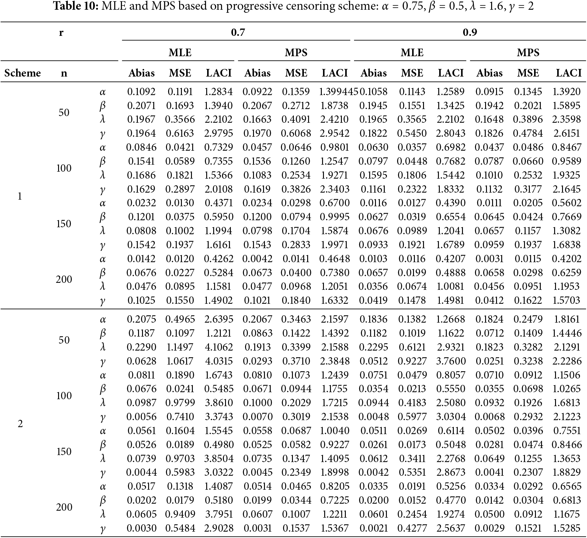
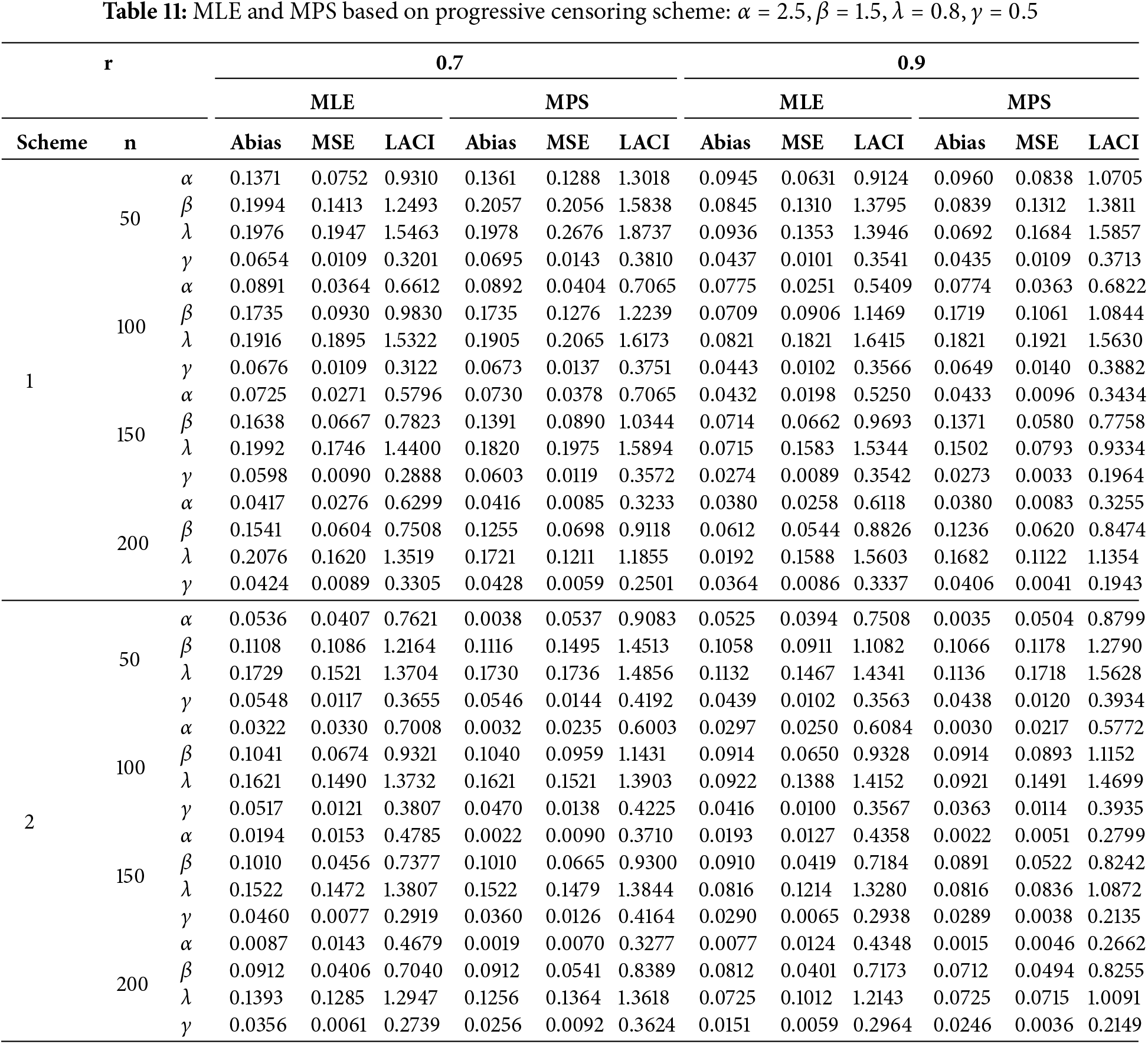
The key observations derived from Tables 10 and 11 are summarized as follows:

1.   Effect of Sample Size: ABias, and MSE decrease as the sample size (n) increases.

2.   Effect of Stages (m): ABias, and MSE reduce as the number of censoring stages (m) increases.

3.   Comparison of Methods: The MLE estimates outperform other methods in most studied cases of the EOEGE-E distribution under progressive Type-II censored samples.

7.4 Application

This subsection presents the application of Maximum Likelihood Estimation (MLE) to estimate the parameters of the EOEGE–E using progressively Type II censored data under different schemes and datasets. Table 12 provides a comprehensive summary of the estimates and their standard errors (StEr) for various parameter values, sample sizes, and censoring schemes.

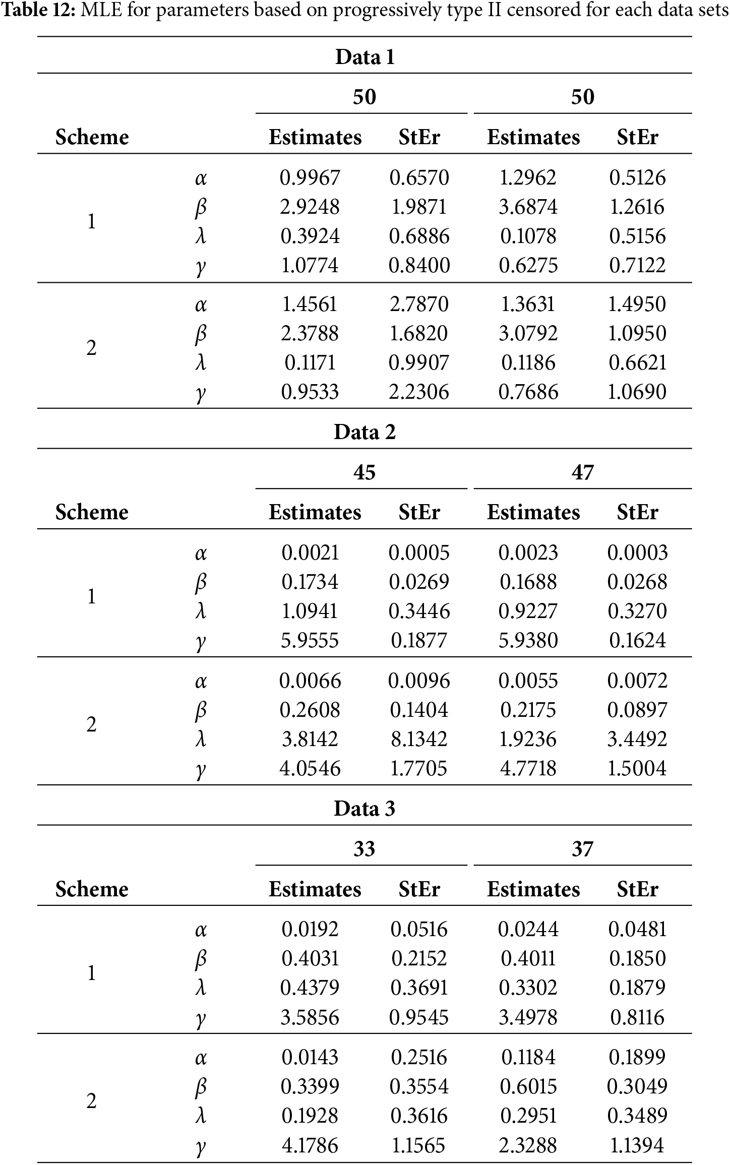
Table 12 presents the application of Maximum Likelihood Estimation (MLE) for parameter estimation under progressively Type II censored schemes across three datasets (Data 1, Data 2, and Data 3) with varying sample sizes and two censoring schemes. The parameters α, β, λ, and γ were estimated, with their corresponding standard errors (StEr) reported. Larger sample sizes consistently improved the reliability of estimates by reducing standard errors, while Scheme 1 generally provided more precise estimates compared to Scheme 2.

8  Conclusion

The Exponentiated Odd Generalized Exponential-Exponential (EOEGE–E) distribution, parameterized by Λ={α,β,λ,γ}, offers exceptional flexibility for lifetime modeling in engineering and medicine. Its versatile PDF and hazard rate functions capture symmetric, skewed, and heavy-tailed data, with skewness from −0.3456 to 3.7012 and kurtosis from 2.1202 to 19.9653. Six estimation methods for complete samples and two (MLE, MPS) for progressive Type-II censoring were evaluated, with MLE showing superior performance. Applied to Datasets 1–4, EOEGE–E achieved excellent goodness-of-fit, modeling material durability, aviation maintenance, medical survival, and electronic reliability. Its robust handling of complete and censored data makes EOEGE–E a valuable tool for reliability and survival analysis. Future work could explore hybrid censoring or competing risks models to enhance its predictive capabilities. The EOEGE–E distribution, despite its flexibility in modeling lifetime data, faces several limitations. Estimating its four parameters (α, β, λ, γ) is computationally intensive, particularly for MLE and MPS, with potential convergence issues in numerical methods like Newton-Raphson for small or censored samples. The study’s focus on Progressive Type-II Censoring limits its applicability to other schemes, such as Type-I or hybrid censoring. Additionally, the EOEGE–E assumes data conforms to its hazard rate shapes, which may not suit highly irregular or multimodal distributions. Future work could explore alternative optimization methods, extend to other censoring schemes, and validate the model across diverse datasets.

Acknowledgement: We express our sincere gratitude to the anonymous reviewers and editors for their insightful and valuable comments, which significantly improved the quality and clarity of this manuscript.

Funding Statement: The authors received no specific funding for this study.

Author Contributions: The authors confirm contribution to the paper as follows: Study conception and design: Zohra A. Esaadi, Rabab S. Gomaa; Data collection: Rabab S. Gomaa, Ehab M. Almetwally; Analysis and interpretation of results: Alia M. Magar, Rabab S. Gomaa, Beih S. El-Desouky; Draft manuscript preparation: Rabab S. Gomaa, Alia M. Magar, Ehab M. Almetwally. All authors reviewed the results and approved the final version of the manuscript.

Availability of Data and Materials: All data generated or analyzed during this study are included in this published article.

Ethics Approval: Not applicable.

Conflicts of Interest: The authors declare no conflicts of interest to report regarding the present study.

Appendix A Derivations

Quantile Function

By inverting the (4), we obtain EOEGE–E quantile function as follows:

xq=[γαlog⁡(1−log⁡(1−q1β)λ)]1γ,(A1)

where q∼uniform(0,1).

Moments

r-th moments of the EOEGE–E distribution are derived by Eq. (9).

E(Xr)=∫0∞xrf(x)dx=αβ∑j=0∞∑i−0∞∑k=0∞(jk)(β−1j)(1+j)iλj+1(−1)j+i+kj!∫0∞xr+γ−1e−α(k−j−1)xγγdx

If, we put

wj,k=∫0∞xr+γ−1e−α(k−j−1)xγγdx(A2)

Then,

E(Xr)=αβ∑j=0∞∑i−0∞∑k=0∞(jk)(β−1j)(1+j)iλj+1(−1)j+i+kj!wj,k(A3)

Substituting z=α(k−j−1)xγγ in (2), we obtain

wi,j,k=(−1)rγ(γ)rγΓ(1+rγ)(1α(k−j−1))r+γγ.(A4)

By Substituting Eq. (4) in Eq. (3), the rth moments of random variable X∼EOEGE−E is

μr′=(−1)rγαβ(γ)rγΓ(1+rγ)∑j=0∞∑i−0∞∑k=0∞(1α(k−j−1))r+γγ(jk)(β−1j)(1+j)iλj+1(−1)j+i+kj!.(A5)

References

1. Marshall AN, Olkin I. A new method for adding a parameter to a family of distributions with applications to the exponential and Weibull families. Biometrika. 1997;84(3):641–52. doi:10.1093/biomet/84.3.641. [Google Scholar] [CrossRef]
2. Ordeiro GM, Lemonté AJ, Cunha DCC. The exponentiated generalized class of distributions. J Data Sci. 2013;11:1–27. [Google Scholar]
3. Gupta RD, Kundu D. Generalized exponential distributions. Aust N Z J Stat. 1999;41(2):173–88. [Google Scholar]
4. Olabad AK. On extended type I generalized logistic distribution. Int J Math Math Sci. 2004;57(57):3069–74. doi:10.1155/s0161171204309014. [Google Scholar] [CrossRef]
5. Olabad AK. On negatively skewed extended generalized logistic distribution. KragujevacJ Math. 2005;27:175–82. [Google Scholar]
6. Olabad AK. On symmetric extended generalized logistic distribution. J Statist Res Iran. 2006;3:177–90. [Google Scholar]
7. Olabad AK. On extended generalized exponential distribution. Br J Math Comput Sci. 2014;4(9):1280–9. [Google Scholar]
8. Alizadeh M, Emadi M, Doostparast M, Cordeiro GM, Ortega EMM, Pescim RR. Kumaraswamy odd log-logistic family of distributions: properties and applications. Hacet J Math Stat. 2014. [Google Scholar]
9. Cordeiro GM, de Castro M. A new family of generalized distributions. J Stat Comput Simul. 2011;81:883–93. [Google Scholar]
10. Maiti S. Odd generalized exponential-exponential distributin. J Data Sci. 2015;13(4):733–54. [Google Scholar]
11. Tahir MH, Cordeiro GM, Alizadeh M, Mansoor M, Zubair M, Hamedani GG. The odd generalized exponential family of distributions with applications. J Stat Distrib Appl. 2015;2(1):1. doi:10.1186/s40488-014-0024-2. [Google Scholar] [CrossRef]
12. de Andrade TA, Bourguignon M, Cordeiro GM. The exponentiated generalized extended exponential distribution. J Data Sci. 2022;14(3):393–413. [Google Scholar]
13. Telee LBS, Karki M, Kumar V. Exponentiated generalized exponential geometric distribution: model, properties and applications. Interdiscip J Manag Soc Sci. 2022;3(2):37–60. doi:10.3126/ijmss.v3i2.50261. [Google Scholar] [CrossRef]
14. Abonongo AIL, Abonongo J. Exponentiated generalized weibull exponential distribution: properties, estimation and applications. Comput J Math Stat Sci. 2024;3(1):57–84. doi:10.21608/cjmss.2023.243845.1023. [Google Scholar] [CrossRef]
15. Aboul-Fotouh Salem S, Abo-Kasem OE, Abdelgaied Khairy A. Inference for generalized progressive hybrid type-II censored weibull lifetimes under competing risk data. Comput J Math Stat Sci. 2024;3(1):177–202. doi:10.21608/cjmss.2024.256760.1035. [Google Scholar] [CrossRef]
16. Almetwally EM, Khaled OM, Barakat HM. Inference based on progressive-stress accelerated life-testing for extended distribution via the marshall-olkin family under progressive type-II censoring with optimality techniques. Axioms. 2025;14(4):244. doi:10.3390/axioms14040244. [Google Scholar] [CrossRef]
17. Elsherpieny EA, Abdel-Hakim A. Statistical analysis of Alpha-Power exponential distribution using unified Hybrid censored data and its applications. Comput J Math Stat Sci. 2025;4(1):283–315. doi:10.21608/cjmss.2025.346134.1094. [Google Scholar] [CrossRef]
18. Balakrishnan N, Cramer E. The art of progressive censoring, statistics for industry and technology. Birkhauser, NY, USA: Springer; 2014. [Google Scholar]
19. Balakrishnan N. Progressive censoring methodology: an appraisal. Test. 2007;16(2):211–59. doi:10.1007/s11749-007-0061-y. [Google Scholar] [CrossRef]
20. Bader MG, Priest AM. Statistical aspects of fibre and bundle strength in hybrid composites. Progress Sci Eng Compos. 1986;1129–36. [Google Scholar]
21. Alotaibi R, Mutairi AA, Almetwally EM, Park C, Rezk H. Optimal design for a bivariate step-stress accelerated life test with alpha power exponential distribution based on type-i progressive censored samples. Symmetry. 2022;14(4):830. doi:10.3390/sym14040830. [Google Scholar] [CrossRef]
22. El-Sherpieny EA, Almetwally EM. The exponentiated generalized alpha power family of distribution: properties and applications. Pak J Stat Oper Res. 2022;18(2):349–67. [Google Scholar]
23. Kamnge JS, Chacko M. Half logistic exponentiated inverse Rayleigh distribution: properties and application to life time data. PLoS One. 2025;20(1):e0310681. doi:10.1371/journal.pone.0310681. [Google Scholar] [PubMed] [CrossRef]
24. Sarhan AM, EL-Baset Abd AA, Alasbahi IA. Exponentiated generalized linear exponential distribution. Appl Math Model. 2013;37(5):2838–49. [Google Scholar]
25. Yan Z, Wang N. Statistical analysis based on adaptive progressive hybrid censored sample from alpha power generalized exponential distribution. IEEE Access. 2020;8:54691–7. doi:10.1109/access.2020.2981497. [Google Scholar] [CrossRef]
26. Al-Essa LA, Eliwa MS, El-Morshedy M, Alqifari H, Yousof HM. Flexible extension of the lomax distribution for asymmetric data under different failure rate profiles: characteristics with applications for failure modeling and service times for aircraft windshields. Processes. 2023;11(7):2197. doi:10.3390/pr11072197. [Google Scholar] [CrossRef]
27. Chesneau C, Yousof HM. On a special generalized mixture class of probabilistic models. J Nonlinear Model Anal. 2021;3:71–92. [Google Scholar]
28. Cordeiro GM, Ortega EM, Popovi’c BV. The gamma-Lomax distribution. J Stat Comput Simul. 2015;85:305–19. [Google Scholar]
29. Lemonte AJ, Cordeiro GM. An extended Lomax distribution. Statistics. 2013;47(4):800–16. doi:10.1080/02331888.2011.568119. [Google Scholar] [CrossRef]
30. Yousof HM, Alizadeh M, Jahanshahiand SMA, Ramires TG, Ghosh I, Hamedani GG. The Transmute-Topp-Leone G family of distributions: theory, characterizations and applications. J Data Sci. 2017;15:723–40. [Google Scholar]
31. Alsulami D. A new extension of the Rayleigh distribution: properties, different methods of estimation, and an application to medical data. AIMS Math. 2025;10(4):7636–63. doi:10.3934/math.2025350. [Google Scholar] [CrossRef]
32. Foya S, Oluyede BO, Fagbamigbe AF, Makubate B. The gamma log-logisticWeibull distribution: model, properties, and application. Electron J Appl Stat Anal. 2017;10:206–41. [Google Scholar]
33. Hussain S, Ul Hassan M, Rashid MS, Ahmed R. Families of extended exponentiated generalized distributions and applications of medical data using burr III extended exponentiated weibull distribution. Mathematics. 2023;11(14):3090. doi:10.3390/math11143090. [Google Scholar] [CrossRef]
34. Suleiman AA, Othman M, Ishaq AI, Abdullah ML, Indawati R, Daud H, et al. A new statistical model based on the novel generalized odd beta prime family of continuous probability distributions with applications to cancer disease data sets. Comput Sci Math. 2022;71:20. doi:10.3390/iocma2023-14429. [Google Scholar] [CrossRef]
35. Oluyede BO, Huang S, Yang T. A new class of generalized modified weibull distribution with applications. Aust J Stat. 2015;44(3):45–68. doi:10.17713/ajs.v44i3.36. [Google Scholar] [CrossRef]
36. Silva GO, Ortega EM, Cordeiro GM. The beta modified Weibull distribution. Lifetidata Anal. 2010;16(3):409–30. doi:10.1007/s10985-010-9161-1. [Google Scholar] [PubMed] [CrossRef]
37. Alizadeh M, Emadi M, Doostparast M. A modified half-logistic distribution: properties and applications. J Stat Res Iran. 2018;15(1):1–20. [Google Scholar]
38. Alizadeh M, MirMostafaee SMTK, Ghosh I. A new odd log-logistic half-logistic distribution with applications to lifetime data. Commun Stat Simul Comput. 2019;50(11):3911–34. [Google Scholar]
39. Al-Shomarni AA, Arif OH, Shawky AI. The Topp-Leone Lindley distribution. J Stat Theory Appl. 2016;15(4):351–66. [Google Scholar]
40. Ozel G, Alizadeh M, Cakmakyapan S. The odd log-logistic Lindley distribution. Commun Stat-Theory Methods. 2017;46(24):12347–64. [Google Scholar]
41. Shaheed G. A new two-parameter modified half-logistic distribution: properties and applications. Stat, Optimiz Inf Comput. 2021;10(2):589–605. doi:10.19139/soic-2310-5070-1210. [Google Scholar] [CrossRef]
42. Shaheed G. A Weighted exponentiated class of distributions: properties with applications for modelling reliability data. Stat, Optimiz Inf Comput. 2025;13(3):1144–61. doi:10.19139/soic-2310-5070-1858. [Google Scholar] [CrossRef]
43. Balakrishnan, Aggarwala R. Progressive censoring: theory, methods, and applications. Berlin/Heidelberg, Germany: Springer Science & Business Media; 2000. [Google Scholar]
44. Ng HKT, Luo L, Hu Y, Duan F. Parameter estimation of three-parameter Weibull distribution based on progressively type-II censored samples. J Stat Comput Simul. 2012;82(11):1661–78. doi:10.1080/00949655.2011.591797. [Google Scholar] [CrossRef]
45. Balakrishnan N, Sandhu RA. A simple simulational algorithm for generating progressive Type-II censored samples. Am Stat. 1995;49(2):229–30. doi:10.1080/00031305.1995.10476150. [Google Scholar] [CrossRef]
Cite This Article
Copyright © 2025 The Author(s). Published by Tech Science Press.
This work is licensed under a Creative Commons Attribution 4.0 International License , which permits unrestricted use, distribution, and reproduction in any medium, provided the original work is properly cited.
Downloads
Citation Tools