
 Submit a Paper
 Propose a Special lssue
 Open Access
ARTICLE
Big Texture Dataset Synthesized Based on Gradient and Convolution Kernels Using Pre-Trained Deep Neural Networks
1 Electrical Engineering Department, College of Engineering, Prince Sattam bin Abdulaziz University, Al-Kharj, 11942, Saudi Arabia
2 Department of Computer Sciences, College of Computer and Information Sciences, Princess Nourah bint Abdulrahman University, Riyadh, 11671, Saudi Arabia
3 Department of Computer Science, College of Computer & Information Sciences, Prince Sultan University, Rafha Street, Riyadh, 11586, Saudi Arabia
4 Department of Computer Engineering, Faculty of Engineering, Arak University, Arak, 38156-8-8349, Iran
* Corresponding Author: Faten Khalid Karim. Email:
Computer Modeling in Engineering & Sciences 2025, 144(2), 1793-1829. https://doi.org/10.32604/cmes.2025.066023
Received 27 March 2025; Accepted 21 July 2025; Issue published 31 August 2025
 View Full Text
 Download PDF
Abstract
Deep neural networks provide accurate results for most applications. However, they need a big dataset to train properly. Providing a big dataset is a significant challenge in most applications. Image augmentation refers to techniques that increase the amount of image data. Common operations for image augmentation include changes in illumination, rotation, contrast, size, viewing angle, and others. Recently, Generative Adversarial Networks (GANs) have been employed for image generation. However, like image augmentation methods, GAN approaches can only generate images that are similar to the original images. Therefore, they also cannot generate new classes of data. Texture images present more challenges than general images, and generating textures is more complex than creating other types of images. This study proposes a gradient-based deep neural network method that generates a new class of texture. It is possible to rapidly generate new classes of textures using different kernels from pre-trained deep networks. After generating new textures for each class, the number of textures increases through image augmentation. During this process, several techniques are proposed to automatically remove incomplete and similar textures that are created. The proposed method is faster than some well-known generative networks by around 4 to 10 times. In addition, the quality of the generated textures surpasses that of these networks. The proposed method can generate textures that surpass those of some GANs and parametric models in certain image quality metrics. It can provide a big texture dataset to train deep networks. A new big texture dataset is created artificially using the proposed method. This dataset is approximately 2 GB in size and comprises 30,000 textures, each 150 × 150 pixels in size, organized into 600 classes. It is uploaded to the Kaggle site and Google Drive. This dataset is called BigTex. Compared to other texture datasets, the proposed dataset is the largest and can serve as a comprehensive texture dataset for training more powerful deep neural networks and mitigating overfitting.Keywords
Today, Artificial Intelligence (AI) tools are widely used in many applications [1–4]. A big dataset is an essential requirement for most novel AI tools, such as deep neural networks. The generation of big datasets has increased significantly over the last decade. Most of these datasets have been provided from raw digital data. Large amounts of digital data are generated by the use of numerous devices and applications, including smartphones, cameras, social networks, satellites, sensors, and others. According to research, approximately 2.5 exabytes were generated each day in 2012 [5]. The IDC (International Data Corporation) reported that 4.4 Zettabytes (ZB) of data were generated in 2013. It is doubling every 2 years. Based on the IDC information, the volume of generated data reached 40 ZB in 2020 [6]. Most of this digital data cannot be used for AI tools. They must be labeled and organized into a specific arrangement to be used as a dataset for AI applications.
Among all types of information, image data plays a main role in most computer vision and AI tools. In other words, one of the most important types of datasets is related to image datasets. A dataset of images can be provided by a camera or smartphone. However, generating the big image dataset is an exhaustive operation. Image augmentation is a common method for increasing the number of images in a dataset. Image augmentation is easier than other types of data augmentation, such as text and voice augmentation [7]. Common methods for increasing the number of images through image augmentation involve changes in rotation, view angle, illumination, size, horizontal or vertical projection, contrast, and image size [8]. The main challenge of these methods is that the generated images are very similar to the original images, and in deep networks, they lack sufficient diversity to train them efficiently. Because these new data do not make fundamental changes in the images, and only some simple visual changes are applied to the original images. One of the most complex types of images, with numerous challenges in image processing and machine vision, is texture. Texture images have a special complexity for processing due to their small and repeating, symmetrical, and asymmetrical structures [9]. Therefore, generating a big texture dataset is more complicated than generating other image datasets.
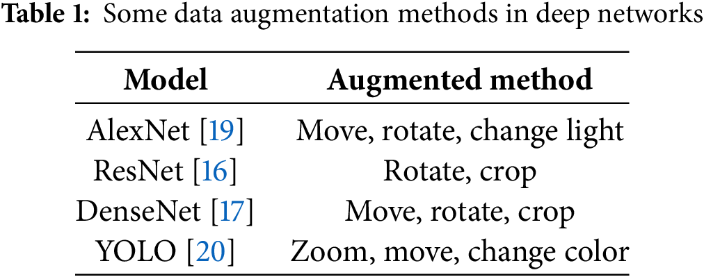
Big datasets can help address some of the challenges associated with training deep neural networks. One of the most significant challenges in training deep networks is overfitting [10]. Different methods have been proposed to mitigate its effects. In recent decades, it has been emphasized that simplifying neural networks and reducing the number of hidden layers or neurons can help solve this problem. However, reducing the number of layers will make the network less powerful and can limit its ability to solve more complex problems. In contrast, increasing the number of layers can lead to overfitting [11]. Several methods have been proposed to address overfitting, including reducing the number of training steps, utilizing evaluation data, randomly removing neurons during training, incorporating a regularization term into the loss function, and employing transfer learning and pre-training networks. However, all of these methods can only partially solve the overfitting challenge in a deep network. The most important and main solution is related to increasing the amount of data and its diversity. Especially discriminative big data that has a high variety and is free of noise and outliers [12]. Today, for training deep neural networks to achieve higher accuracy, a big dataset is much more necessary than in previous years [13]. Preparing big and diverse data is one of the significant challenges for artificial intelligence tools, such as deep neural networks [14]. Without sufficient data, not only are deep neural networks not useful, but they also cause the problem of overfitting and high error rates in the test data. As mentioned earlier, the key method to address this challenge is to increase the amount of data [15]. If the amount of data is not enough, this number can be increased using techniques such as data augmentation. In most deep networks, data augmentation methods have been utilized to increase the image data. Table 1 lists some deep networks [16–20] that employ various methods to augment their data.
In general, image augmentation methods are divided into three groups: model-free, model-based, and optimization-based methods. The first category, namely model-free methods, utilizes image processing techniques, while the model-based approach employs image generation models to combine images. On the other hand, methods based on optimization aim to find an optimal combination of images [21]. In most image datasets with labels, image augmentation can alter the label of an image, posing challenges in training the networks. Xu et al. reviewed several image augmentation techniques [8] to generate new image classes. Takase et al. [22] proposed Self-Paced Augmentation (SPA), which automatically selects the best samples for data augmentation by training a neural network. It increases the generalization of the data. Bochkovskiy et al. [23] provided the YOLOv4 (You Only Look Once) framework for object detection. In this research, image augmentation is achieved through the linear integration of other images. Hendrycks et al. [24] proposed a method that first generates several images from a single image and then produces a new image by combining those images. Dwibedi et al. [25] proposed a method for separating objects from the background. In this approach, new images are generated by replacing the backgrounds. This technique, known as copy-paste [26], is widely employed to generate new images. Baek et al. [27] presented a method based on mask optimization that combines two images using statistical information. They generated a new image from two images. First, each pair of images is divided into smaller pieces. Then, the pieces are spatially combined, and the edges of each part are linearly merged. Li and Wand [28] proposed a method that combines a generative Markov random field and trained deep convolutional neural networks (dCNNs). The Markov random field operates at higher levels of a dCNN feature pyramid and determines the texture layout to enhance visual scenes.
As mentioned earlier, texture images are more complex than general images. Therefore, generating the texture includes more challenges. There are two main techniques for texture generation. The first methodology involves creating a new texture by using individual pixels or patches from the original texture [29]. These non-parametric techniques can produce high-quality textures [30]. However, these methods do not establish a formal model for natural textures. The second type of methodology for texture synthesis is related to the parametric texture models. These methods include a collection of statistical measurements derived from the spatial dimensions of the image. This framework provides a texture characterized by the results of the measurements, and any image that has the same results belongs to the same texture. This approach was initially proposed by Julesz, who indicated that a visual texture can be uniquely represented by the Nth-order joint histograms of its pixels [31]. One of the most effective parametric models for texture synthesis was introduced by Portilla and Simoncelli [32]. This model used a set of statistical coefficients corresponding to basis functions at adjacent spatial locations, orientations, and scales.
Another novel technique to generate high-quality texture is self-tuning. This technique was introduced by Kaspar et al. [33]. They introduced a novel approach to generating high-resolution textures from limited exemplars. This method employed self-tuning texture optimization to address key challenges in texture synthesis, including maintaining visual fidelity and avoiding repetitive patterns. This technique concentrates on three challenges of texture synthesis. Irregular large-scale structures are faithfully reproduced through the use of automatically generated and weighted guidance channels. Also, repetition and smoothing of texture patches are avoided by new spatial uniformity constraints. Finally, a smart initialization strategy is employed to enhance the synthesis of regular and near-regular textures, without compromising textures that do not exhibit regularities. Qian et al. [34] proposed the Self-similarity matching method to synthesize exemplars of textures, performing distance error matching and alignment via the sum of self-similarity. This method expands the search range of the suture from one patch to all patches in the horizontal direction, eliminating the broken features of overlaps in the outputs. Dong et al. proposed an exemplar-based method [35] for texture synthesis based on support vector machines. They improved the texture synthesis methods based on patch sampling and pasting. It can generate realistic textures with a similar appearance to a small sample. However, the sample usually must be used throughout the synthesis stage. In contrast, the learned representation of the textures is more compact and discriminative, and can also yield good synthesis results. This approach benefits from the merits of Support Vector Machine (SVM), which allows the sample texture pattern to be learned using a model, and the sample itself can be discarded during the synthesis stage. The approach is also utilized to synthesize three-dimensional surface textures. Yang et al. [36] employed the Self-tuning technique with a transfer dynamic convolution autoencoder to predict quality prediction features. This method extracts inner dynamics and utilizes private spatiotemporal information.
In recent years, generative deep neural network models have achieved remarkable results in texture synthesis. Goodfellow et al. [37] are the pioneers in developing Generative Adversarial Networks (GANs) for this purpose. These networks consist of two distinct components: a discriminator and a generator, with various implementations developed for generating new data. Mirza and Osindero proposed the Conditional GAN (CGAN) [38], which allows for the generation of new images by incorporating target information (labels) into both the training and generated images. Kim et al. [39] introduced a generative neural network known as spatial GAN (SAGAN), which is utilized for producing geological texture images. An important property of this approach is related to its capability to generate large-sized textures. Bergmann et al. created larger images by selecting patches of texture and replicating them alongside other textures [40]. This method cannot generate new texture patterns because it only replicates the previous patterns. Accordingly, some approaches employed covariance-based techniques for creating and analyzing texture heterogeneity [41].
Guan et al. [42] developed Texture-constrained Multichannel Progressive GAN (TMP-GAN) to enhance medical images by using textures. They introduced a generation method to decompose the challenge of augmentation. Zdunek [43] proposed a hybrid texture synthesis method for interpolating image structures to facilitate texture combination. This method cannot generate an image entirely; however, it generates the missed regions of each texture. This method combines radial basis function interpolation with texture synthesis to generate incomplete parts of textures. Radford et al. developed a deep convolutional GAN (DCGAN) neural network for generative networks to stabilize the training process against variations in its parameters [44]. Jetchev et al. presented a model of a spatial generative adversarial network (SGAN) [45] that efficiently uses only convolutional layers, without fully connected layers, to generate the texture. Although this method operates very fast, it encounters some challenges in determining the texture types. Fan et al. [46] proposed a texture synthesis method based on texture optimization. This method employs global optimization to address the challenge of non-homogeneous texture synthesis. It increases the convergence rate and enhances the quality of texture synthesis. Some papers, such as [47], proposed a novel approach for generating textures of infinite size by using Generative Adversarial Networks (GANs) based on a patch-by-patch paradigm. It utilized spatial stochastic modulation to allow for local variations and improve pattern alignment in the large image. Salari and Azimifar [48] proposed a hybrid model to improve the quality of generated textures. They combined the Vision Transformers (ViTs) with SGAN and used a self-attention mechanism to capture long-range dependencies in textures.
Generative adversarial networks have some limitations. These types of networks include two deep neural networks, and the training step requires high computational complexity. Therefore, the process of image generation is relatively slow. In addition, they can generate only a similar texture to the original images. Hence, Fan et al. [49] enhanced the VGG network by adding batch normalization layers to improve the texture generation speed. Also, they applied noise to the original images to make changes in the output images compared to the original textures. In addition to Generative Adversarial Network (GAN) methods, traditional approaches such as Hidden Markov Models [50] and various non-parametric techniques [51] were proposed for texture generation. However, these methods have more limitations and challenges compared to deep neural networks. Using pre-trained networks is another technique to address some limitations of GAN methods. Pre-trained networks have played a crucial role in deep learning [52]. Due to the limitations of memory and processing units, it is not possible to train most big datasets on general hardware. The pre-trained networks address this challenge in most AI applications [53–55]. In this study, some pre-trained networks are employed to generate a new class of textures. All of the networks used in this study are trained on the ImageNet dataset [56], which includes 1000 classes of image data. Some of these networks are VGG [19], Xception [57], ResNet [16], and DenseNet [17]. This study utilizes VGG16, ResNet152, and DenseNet169 to generate an example of a big dataset of textures.
This study proposes a deep neural network-based approach that offers several advantages over GAN methods. One important advantage is that, unlike adversarial networks, this approach does not require original images for training. In addition, the generated textures have a higher quality than those produced by the GAN methods. In terms of speed, the proposed method can provide the output textures rapidly. The speed of this operation is considerably greater than that of adversarial neural networks.
The rest of this paper is organized as follows: Section 2 describes the models of texture generation and presents the local binary pattern (LBP) [58]. It is a texture descriptor employed to distinguish between complete and incomplete textures. Section 3 develops the proposed methods. Experimental results and conclusions are reported in Sections 4 and 5, respectively.
This section reviews various types of image augmentation methods is done. Another part of this section is related to a texture descriptor that is used in the proposed method.
Model-free methods refer to those that do not utilize a model for image augmentation. These approaches perform image augmentation by using one or several images. It can be achieved through translation, color and brightness adjustments, and geometric transformations. Some methods perform image augmentation using one image, such as Hide-and-Seek [59], GridMask [60], Cutout [61], and Random Erasing [62]. However, other techniques use several images to generate a new image. Some of the most important research related to these techniques is Sample Pairing [63], CutMix [64], Mixup [65], BC learning [66], and AugMix [24].
In general, model-based methods are often equivalent to generative models. These methods perform image generation based on a generative model and a discriminative model. These methods are time-consuming and can be divided into three types [27]. Some methods are unconditional, the second type is conditional on the label or class, and the third type is conditional on the image itself. If the images have no class or label, their generation is unconditional, as seen in models such as the Deep Convolutional Generative Adversarial Network (DCGAN) [47] and CutPas [67]. When the images have a class, it is necessary to use conditional types. These methods can preserve the image label after data augmentation, such as AugGAN [68], or in some cases, the class of the new image is changed, such as GAN-MBD [69] and EmoGAN [70].
2.3 Methods Based on Optimization
These types of image augmentation methods can be done by reinforcement learning approaches [71] or generative adversarial networks [72]. The first method uses reinforcement learning to determine the optimal strategy, while the second type employs generative adversarial networks (GANs). GAN-based methods can be applied to both model-based and optimization techniques. The goal of model-based methods is to directly generate images, whereas the optimization method [73] utilizes an optimizer to minimize the loss function, providing better images. There are papers based on reinforcement learning, such as BPA [74], MADAO [75], Faster AA [76], Rand Augment [77], and LDA [78]. In addition, some researchers have proposed techniques based on adversarial networks to generate images, such as CDST-DA [79], ADA [80], and Ada Transform [81].
2.4 Methods Based on Image Processing
These methods are special types of model-free techniques for image augmentation. However, because of the importance of these approaches in this section, the details of these methods are discussed. The image augmentation based on image processing can be divided into the following techniques [82].
The flip for image augmentation can be horizontal or vertical. Horizontal flipping is much more common than vertical flipping. Because it can generate incorrect images due to vertical projection. This method is one of the easiest ways to increase images [9].
Applying changes to the color channels is another method for generating new images. The change in color involves some steps. First, separate the color channels, such as R (red), G (green), or B (blue). In addition, the RGB values can be easily adjusted through image processing operations to alter the image’s illumination. The color changes should not alter the classification of the data. For example, the leaves of the tree should not change to a blue color [27].
Image cropping can be performed as a step in image processing and transformation to resize images to different dimensions. Random cropping can be utilized to generate new images. This change can remove useful information from the image. In addition, most datasets require the exact image size. Therefore, to maintain the size of the image, the size of the cropped image must be enlarged, or the empty areas must be filled with data from the adjacent parts [22].
One of the most effective and straightforward ways to increase image data is through rotation. This method is performed by rotating the image on an axis between 1 and 360 degrees. The degree of rotation should be determined by the degree of rotation parameter. Minor rotations in the negative and positive limits can be useful for most tasks, but as the degree of rotation increases, the image label cannot be preserved. Therefore, the important point is that the rotation should not be greater than a threshold value. For example, a ball can be rotated to any degree, but some images must be rotated at a maximum of 20 or 30 degrees. Because in reality, for example, there is no vertical car [22].
Moving images left, right, up, or down can be useful for generating new images. For example, if the images in the dataset are centered, such as in face datasets, they can be augmented by shifting. When the original image is shifted in one direction, the empty space can be filled with a fixed or random value, or the values of neighboring points can fill it. The important point is that incorrect information can be created in the background of the image due to displacement, which should be corrected [21].
This method adds random noise to the image using a noise matrix, which is typically drawn from a Gaussian distribution. Adding noise to images can help networks learn noise-tolerant features [9]. It is important to apply a low level of noise to preserve the local details of the image.
Images can be zoomed in or out. This zooming can make the image smaller or larger. The zoom operation is performed digitally, and image quality can be enhanced with various image processing methods, such as interpolation and more advanced techniques [22].
Convolution is a popular operation in image processing that allows for the application of special effects to images. The effect of convolution is related to the kernel or filter used. The convolution filter can be divided into two categories: low-pass and high-pass. The first category removes noise by smoothing the image. It also removes some details and edges. The second type increases the sharpness of images. In deep convolutional networks, these types of filters play a significant role in extracting features from input images. This study uses these filters by combining them with an ascending gradient to produce textured images. In common methods, applying a filter or convolution mask to the image only makes minor changes in the edge or local information of the image and does not create a new image. However, in the proposed method, a new textured image is created [83].
This method is complex and has some challenges. Combining two images can be done by using the average of their pixels. However, it is a less common approach for image augmentation. The images produced by this approach cannot appear naturally and do not convey the correct sense to a human [30].
The proposed method introduces a novel approach to generating new textures. This section reviews a robust texture descriptor, which plays a vital role in many aspects of the proposed algorithm.
The Local Binary Pattern (LBP) [58] is an effective statistical technique for extracting features from textures. There are other well-known texture descriptors such as the Gray Level Co-occurrence Matrix (GLCM) [84]. However, despite the LBP, GLCM is sensitive to illumination and rotation. LBP has been used in various applications, including facial recognition [85] and medical image analysis [86]. The first LBP operator was introduced by Ojala et al. [85]. It involves generating binary codes based on comparing P points from neighboring pixels with the central pixel. A binary code of 0 is assigned if the value of the neighboring pixel is lower than that of the central pixel; otherwise, it is set to 1. Then the binary code is multiplied by the corresponding weights and combined to produce the LBP code. The calculation of LBP value is expressed in Eq. (1):
where
Fig. 1 illustrates the calculation of the LBP code. This example uses the square neighborhood that is not rotation-invariant. The circular neighborhood must be utilized to provide the rotation-invariant property. Different versions of LBP have been proposed, and most of them are not rotation-invariant. Therefore, the original LBP was developed to
where riu2 is the rotation-invariant uniform patterns [88]. These patterns have U = 0 or U = 2. The calculation of U is illustrated in relation 5. The U value indicates the measure of uniformity. It represents the number of transitions, specifically the bitwise 0/1 alterations between adjacent bits within the circular structure. Fig. 2 illustrates some uniform and non-uniform patterns. Most patterns of general textures are uniform, and these patterns play a critical role in the extraction of texture features.
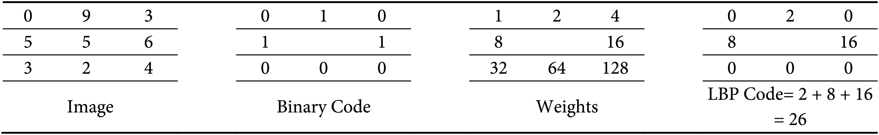
Figure 1: Process of calculating the LBP code
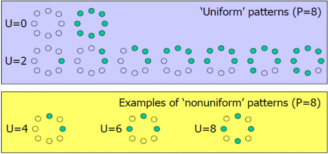
Figure 2: Uniform (U = 0 and U = 8) and non-Uniform Pattern for P = 8 neighborhood
Relations 3 to 5 indicate the LBP_S (sign LBP) with mapping of riu2. In Step 3-1 of the proposed method, LBP_M (magnitude LBP) is used [89]. LBP_M is the same as LBP_S, but it compares the difference between the center and each neighbor point to a magnitude threshold. LBP_S, LBP_M, and LBP_C (center LBP) combine together, and CLBP (complete LBP) is made [89].
3 Proposed Method and Parameters
This section discusses the proposed algorithm and its parameters.
This section describes the proposed framework. This framework can generate a new texture dataset based on some pre-trained deep neural networks. The proposed method consists of five steps, with the primary step being the second one. The entire steps are given in Table 2. It includes two main parts. In the first part (steps 1–3), a new class of texture is generated. In the next part (steps 4 and 5), this new texture is reproduced through image augmentation and saved in each class.
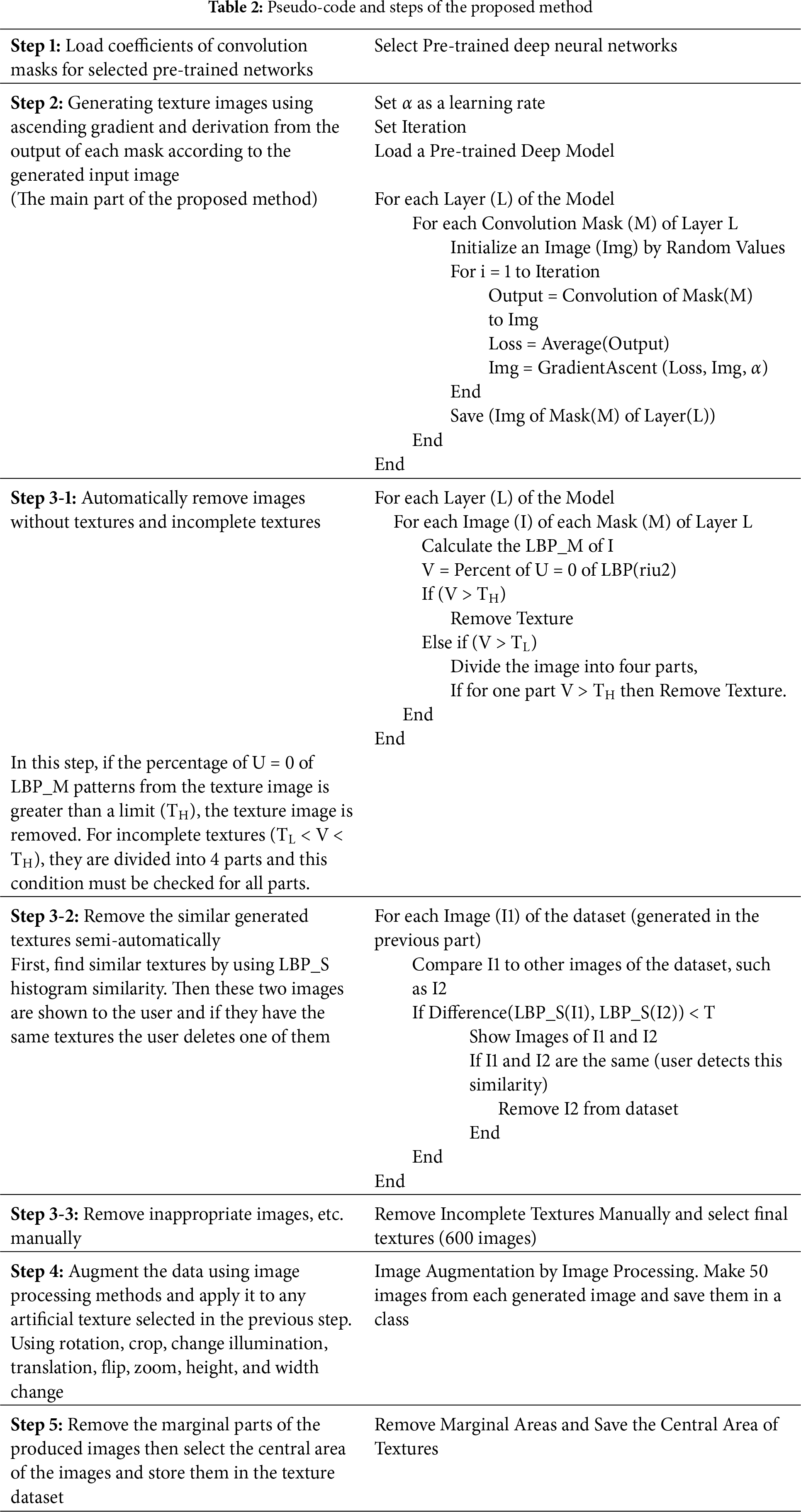
The proposed framework combines gradient optimization and image augmentation. In this method, texture images are created in steps 1 and 2. Some incomplete and similar generated textures are automatically and semi-automatically deleted by the proposed techniques in step 3. Then, in the 4th step, the image augmentation operation is performed to increase the number of images for each texture class. In some research [83], the gradient technique is applied to the output of convolution masks. Each of the convolution masks is utilized to display the extracted features and to generate a heat map of the classified images. It displays the important parts of the image to determine the image’s class [90]. The convolution kernels of several pre-trained neural networks, such as VGG16, DenseNet169, and ResNet152, are utilized to extract the texture patterns of each image. These networks are trained on the ImageNet dataset [20], and their convolutional parameters are utilized for texture generation.
A layer of a pre-trained network is selected in each loop of the proposed algorithm. This layer has some masks or convolution kernels. One of these kernels is selected for each run of the main loop. In the main loop of the algorithm, a random image is generated. Then, the output of the convolution operation using the selected kernel and this image is employed for the gradient ascent operation. In each iteration of this loop, this image is changed to increase the output of that kernel. The gradient of the output of the convolution mask is calculated relative to this image. In each loop, this gradient must be increased. The loss function is the sum of the output values of the convolution operation. This value increases in a loop by changing the image using an ascending gradient. These changes eventually lead to generating a new texture image. A loop with sufficient repetition (100 times) is applied to the initial random image, and a new texture is generated.
Each kernel extracts some features of the input image. If the input image does not possess those features, the output kernel is inactive for those features. In addition, some kernels of a pre-trained network cannot provide good coefficients due to low iteration loops and training operations. Therefore, these kernels cannot generate texture, and the output image is not a texture. An example of this output is shown in Fig. 3. Some kernels only extract the color information of an image, as illustrated in Fig. 3b. In addition, some output images can include incomplete textures, such as Fig. 3c–e. All of these inappropriate textures are deleted in step 3-1 automatically.
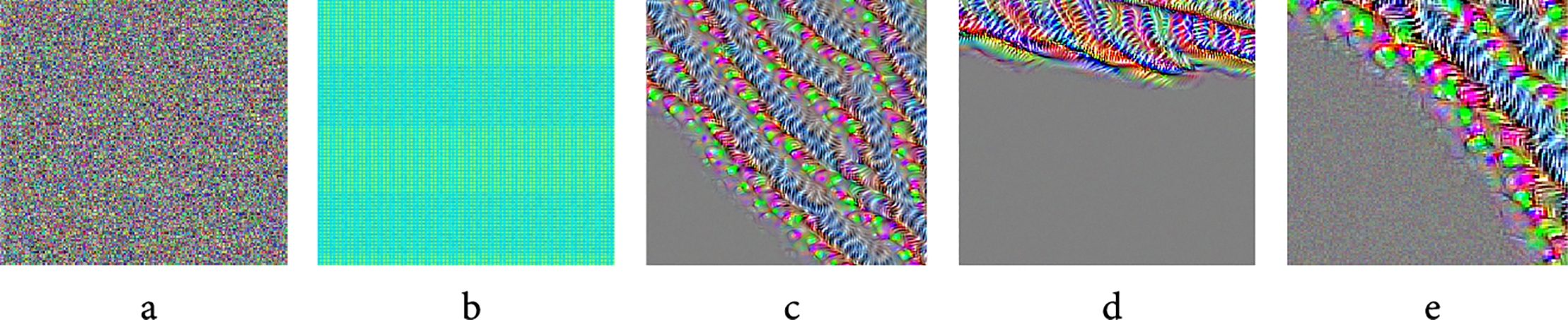
Figure 3: Sample images that are automatically deleted in step 3
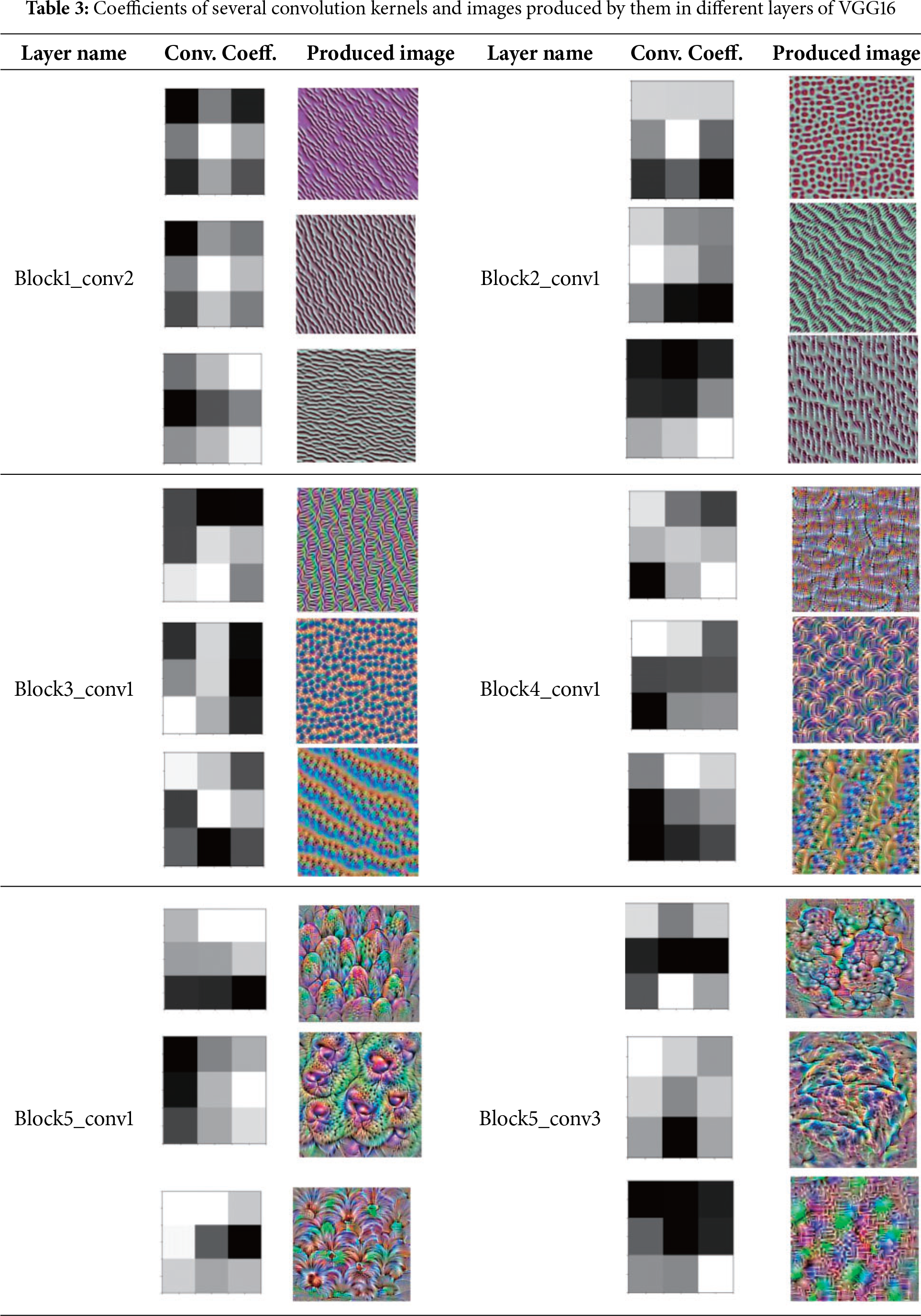
A pre-trained network includes different layers. The layers near the output of a deep network have more specific features; therefore, they can contain more inactive kernel outputs. This is because most of the specific features can not exist in input images. These outputs cannot provide complete textures, such as in Fig. 3. Fig. 3a shows an example of the output of an inactive kernel. For example, in the VGG16 network, the block4_conv2 layer, one of the last convolutional layers, includes 330 inactive kernels. This layer has 512 kernels. This study presents an automatic method in step 3-1 to detect and remove these images. Table 3 lists examples of VGG16 kernels and their corresponding output textures. As it is mentioned in most of the research, such as [83], the initial layer of each deep network extracts general features, such as points, edges, lines, and others. When the data feedforward through the network, the features (the output of each convolution layer) are changed into more specific features. In other words, the features of convolutional layers that are near the output are more specific than those of previous layers. Table 3 indicates that the texture features of the initial layers are fine, whereas the textures of the layers near the output are more specific and include more complicated patterns. Therefore, in the proposed method, most of the textures were extracted from the last convolutional layers. In addition, the features that belong to the near layer are similar to each other; therefore, the layers that are far from each other are employed in the proposed method. The more specific features, the more inactive output can be provided by the main loop of the proposed method. This is because most of the images cannot include some of the specific features; therefore, the output of the loop cannot generate those features (textures). An automatic technique is proposed in this study to detect inactive textures, such as the one shown in Fig. 3a (Step 3-1).
An automatic method is proposed to detect incomplete or inactive output. Based on some research [91], the percentage of uniform patterns in general textures is higher than in other images. Therefore, the proposed method (in Step 3-1) uses this fact to detect the incomplete textures or inactive kernel outputs. Fig. 2 shows that the uniform patterns include patterns with U = 0 and U = 2. Generally, the high percentage of uniform patterns belongs to U = 2. The implementations indicate that for incomplete textures or inactive kernel outputs (such as those in Fig. 3), the high percentage of uniform patterns corresponds to U = 0 rather than U = 2. Therefore, this study employed it to detect incomplete textures. In addition, LBP_M offers better distension than LBP_S for this purpose. Therefore, in this step, LBP_M is employed to detect incomplete textures.
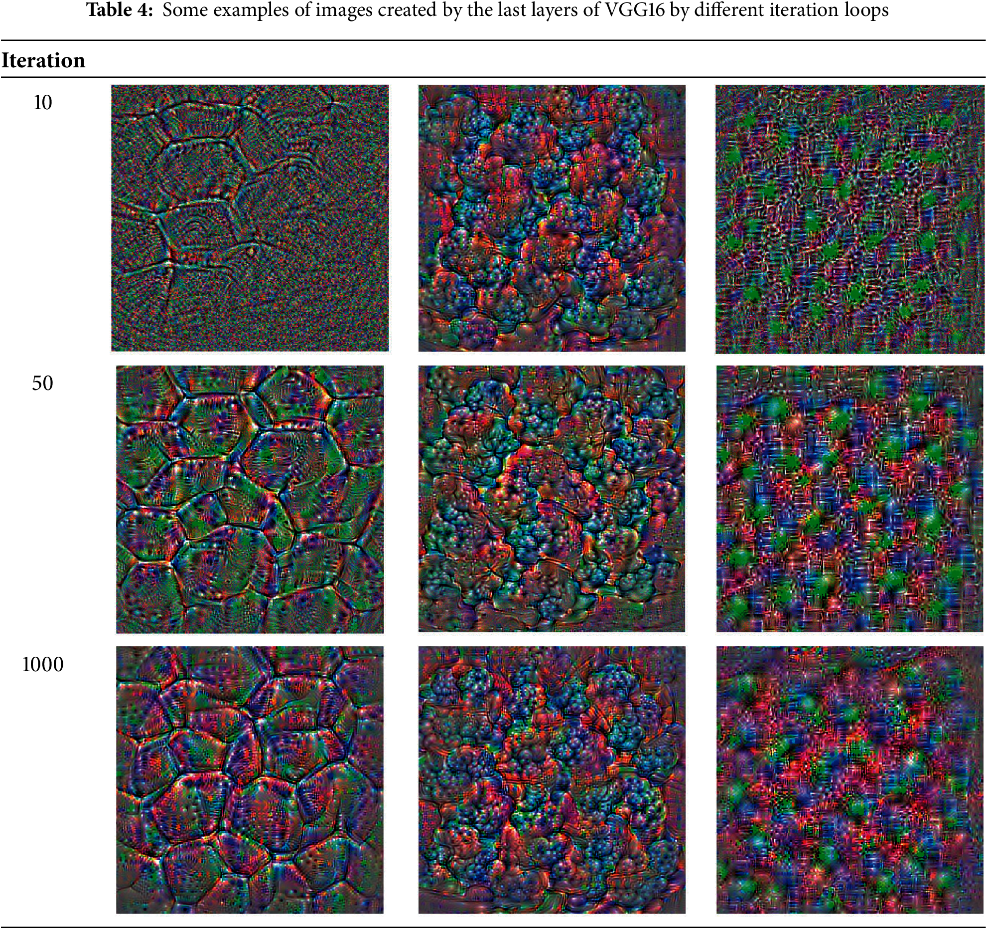
The analysis of the LBP_M indicates that the higher percentage of the U = 0 belongs to the smooth non-texture area. In other words, the incomplete textures include a higher percentage of U = 0 than general textures. At the beginning of step 3-1, the local binary pattern is calculated for the generated texture, and then the percentage of uniform patterns with U = 0 is determined. If this percentage exceeds a specific limit, the texture is not generated well and is removed automatically. Some of these images, along with the percentage of U = 0, are illustrated in Fig. 4. It shows some non-texture images with different histograms. The sum of the first and last bins of uniform patterns (patterns with U = 0) of these images is higher than a threshold value. (00000000 and 11111111 LBP codes for P = 8). Therefore, they are removed in this step. Fig. 5 shows different selected textures and their histogram of uniform parts of LBP. This figure is related to an LBP (riu2) with R = 1 and P = 8. Fig. 5 indicates that for all texture images, the percentage of patterns with U = 2 is higher than U = 0. These textures are selected automatically in step 3-1. Fig. 4 indicates that the percentage of U = 0 patterns of these images is greater than T_H. Therefore, they are removed in step 3-1 automatically. Some images, such as Fig. 3c–e, illustrate incomplete textures. For these images, the percentage of U = 0 patterns can be between T_L and T_H. These images are divided into four parts, and if the percentage of U = 0 patterns is higher than T_H for one or more parts, the images are removed. It is possible to divide images into 3 × 3 or more parts and check this condition to remove incomplete texture precisely. T_H and T_L are two threshold values to detect incomplete textures. In this study, T_H is the average value of the two largest values in the LBP_M histogram and T_L is 0.6 × T_H. In step 2, the iteration value is set to 100. The incomplete textures, such as Fig. 3c–e, can be removed or the iteration value increased to provide a complete texture. Table 4 shows examples of images generated by the last layers of VGG16 based on the number of different iteration loops.
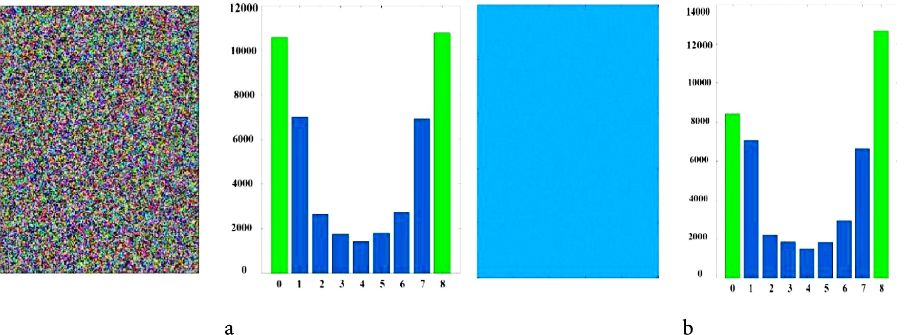
Figure 4: Removing incomplete textures automatically (Step3)
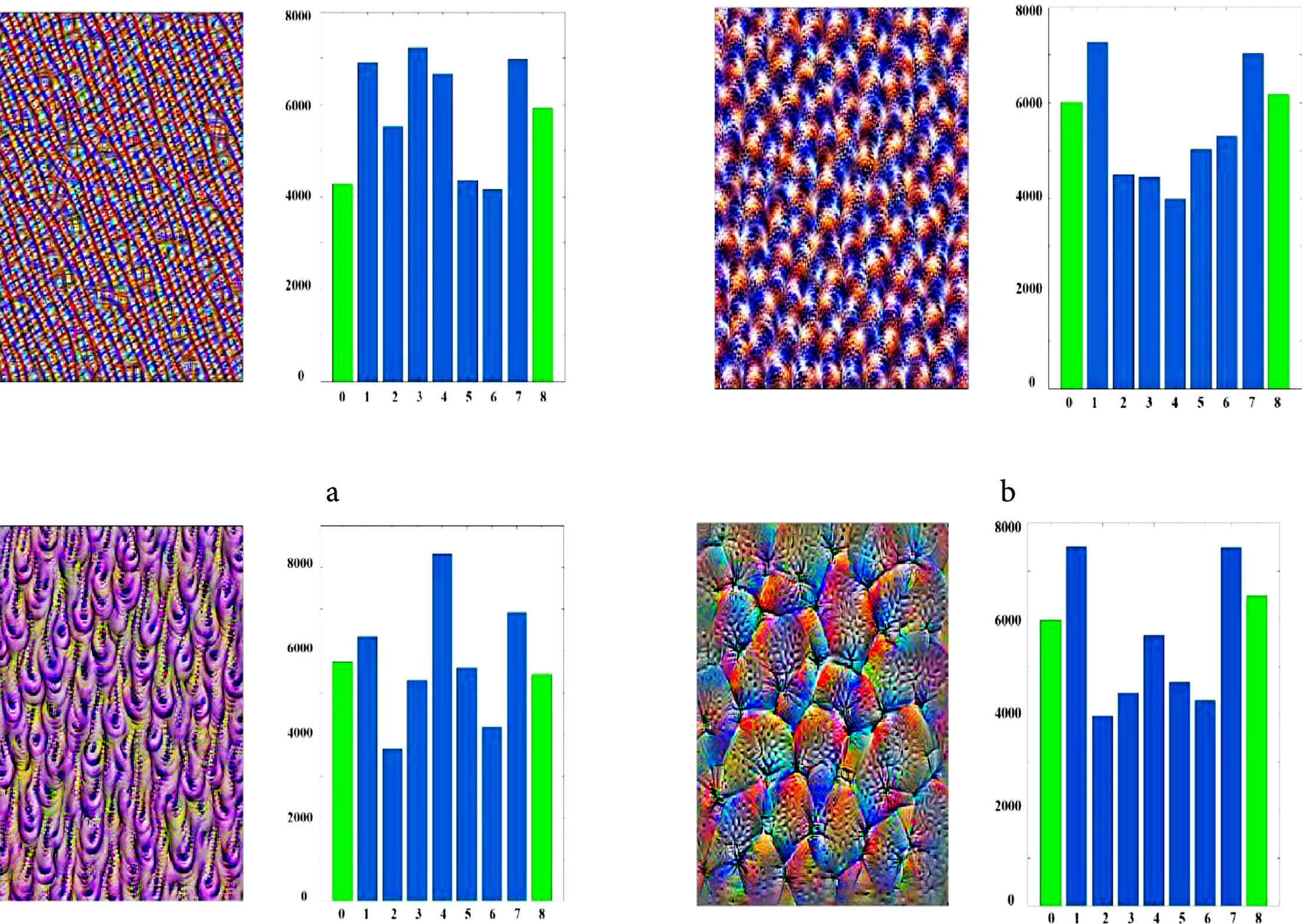
Figure 5: Selection of completed textures (Step3)
After removing the incomplete textures, the similar generated textures must be removed. This operation is performed semi-automatically in step 3-2. Each kernel of each layer of a pre-trained network can generate a new class of texture. However, some similar kernels, especially in the two near layers, can generate similar textures. Therefore, the proposed method does not use the kernels of all layers for texture generation. The employed layers must be spaced far apart to generate different textures. However, it is possible to produce two similar textures from two different kernels. In step 3-2, these similar textures are determined and removed semi-automatically. For this purpose, all of the generated textures after step 3-1 are compared to each other by using LBP vectors. If the difference in LBP vectors between two textures is lower than a threshold, such as T, these textures are displayed to the user, and the user removes one of them if they are visually similar. It is possible to use the strict threshold to automatically remove most similar textures without user supervision. However, a strict threshold can remove some different textures. This is because, in some cases, two different textures can provide nearly or similarly similar LBP feature vectors.
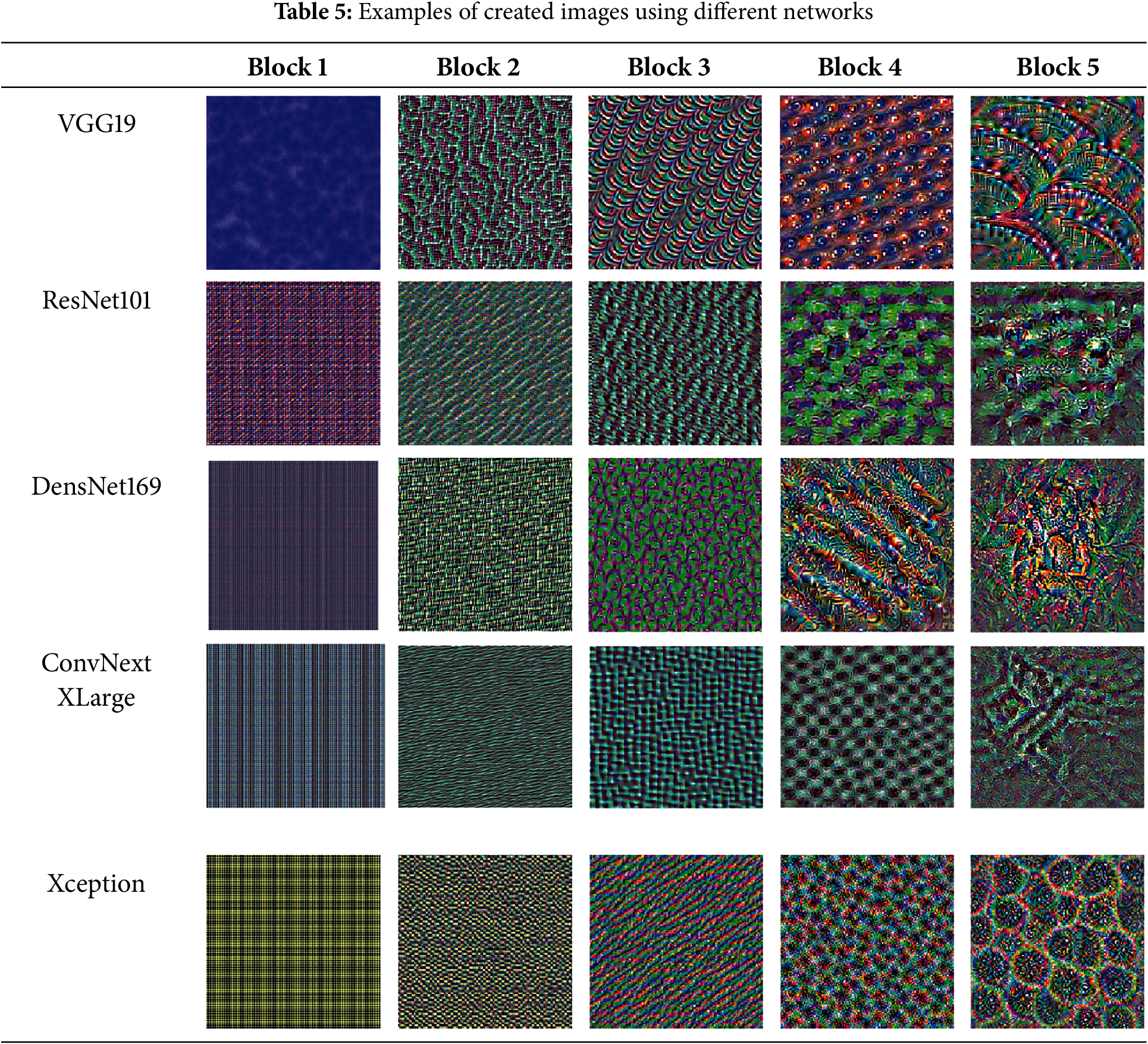
At the end of the third step in step 3-3, the user manually deletes some textures, and finally, 600 textures are selected to generate the dataset. Table 5 presents examples of these images for various layers of different networks. It indicates that some images contain finer and more general texture patterns. These images are generated by using the convolution channels close to the input layer. On the other hand, the images obtained from the convolution layers near the output layer are more complex. This is because these images contain more specific features.
In the fourth step of the proposed method, image augmentation is employed to enhance texture. This step involves various operations, including rotation, light adjustment, contrast adjustment, horizontal flipping, zooming, and others. Table 6 lists all image modification methods used in the augmentation part.
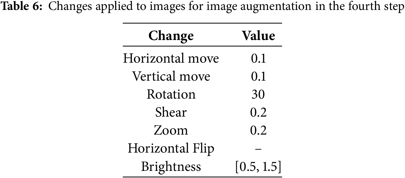
Image augmentation applies the transformations to each image without changing its semantic content. Such transformations are performed randomly or systematically at the training step. Common augmentation techniques that can be applied to images include geometric transformations such as rotation, flipping, cropping, translating (or shifting), and zooming. Another technique for enhancing images is through color transformations. Adjusting brightness, contrast, hue, and saturation are just a few examples. Noise injection is another method of image augmentation that can be used with Gaussian noise or speckle noise for this purpose. However, it can decrease the quality of the textures. Therefore, it is not used in this study. There are some more advanced techniques for image augmentation. Cutout is a technique that masks out random patches of the image. Mixing methods combine two images into one. The image augmentation should preserve the label of each image.
In the proposed method, image augmentation causes some challenges in images. As a result of rotating, shifting, or zooming (shrinking) the image, some empty spaces appear, which common data augmentation methods fill inappropriately, as seen in the images in Fig. 6. The margins of the generated image are removed by 50 pixels on each side, and the central area of each image is selected as the final texture for the dataset, addressing these problems in the last step. As a result, the 250 × 250 images are resized to 150 × 150 and stored in the final dataset.
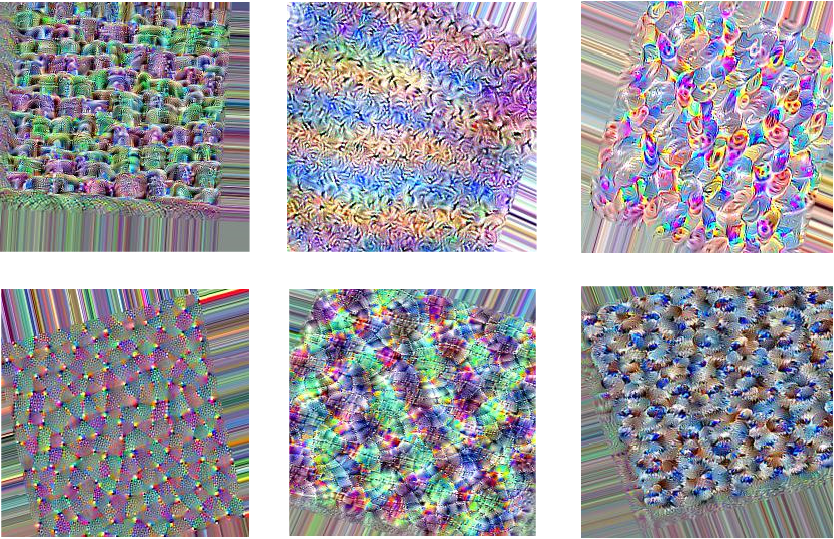
Figure 6: Some images from step 4
3.2 Discussion of Proposed Method
The loop operation is applied to all the masks of different convolutional layers, and the resulting images are saved. At the end of the application of the loop, there is a set of images, each of which corresponds to a convolution layer, and each contains a number of images equal to the number of channels or filters of each layer. Only a subset of kernels is selected from each layer. The closer the convolution layer is to the input layer, the finer and simpler the textures in the generated images are, and the images of the last convolution layers are more complex.
3.3 Some Important Points to Generate Textures
• If the kernel belongs to the first layers of the deep network, the output image in step 2 has finer textures or is textureless. In other words, the kernels belonging to the last layers provide textures with more details and more complex patterns. This is because the initial layers of convolution extract more general features, while the later layers extract more specific features. It is shown in Tables 3 and 5.
• The kernels of the first layers of different pre-trained networks provide general features. In other words, they generate the same output. The outputs often include only color or very fine textures. Therefore, in step 2, most of the kernels of the last layers (near the output layers) are used because these kernels provide more specific features, and for different networks, they provide different textures.
• The peer kernels of the two near layers in a deep network generate similar textures. Therefore, in step 2, for each block (which includes some layers), only one layer is utilized to generate texture.
• The significant number of kernels in each layer is inactive and does not generate texture images. The closer layer to the output, the number of inactive kernels increases significantly [83].
• Each kernel of the convolutional network not only extracts the details of the edges and structures of input images but can also extract their colors. Therefore, to create a texture dataset, it is necessary to pay attention to it. In other words, it is necessary to remove similar textures with the same structure and colors.
• Fig. 3c–e indicate that some outputs of step 2 include incomplete textures. The “Iteration” value that determines the repeating time of the main loop in step 2 should be increased to complete these types of textures. However, increasing this value significantly increases the computation time. Instead of increasing the loop execution time, these incomplete textures are automatically detected and removed in step 3. The Iteration value is set to 100 to provide fast operations. Table 4 indicates some of the outputs with different “Iteration” values.
• As mentioned in some studies, such as [83]: “The first layers act as a collection of various edge detectors. At that stage, the activations retain almost all of the information present in the initial picture. The activations become increasingly abstract and less visually interpretable when they go deeper. They begin to encode higher-level concepts such as “cat ear” and “cat eye.” Deeper presentations carry increasingly less information about the visual contents of the image, and increasingly more information related to the class of the image. The sparsity of the activations increases with the depth of the layer: in the first layer, almost all filters are activated by the input image, but in subsequent layers, an increasing number of filters remain inactive. This means the pattern encoded by the filter is not found in the input image” [83]. When a kernel is not activated during the training step, it means it cannot extract significant features for an input image. Some of these kernels can be activated, but they are not fully activated. Therefore, they do not include good coefficients. In other words, these kernels cannot generate complete textures.
• The closer the kernel is to the output layers of the network, the greater the possibility of producing incomplete textures, because as the input image progresses through the network layers, the extracted features become more specific and move away from a general state. As a result, the probability of a kernel being disabled increases because the kernel depends on more specific features, and some of these features cannot be present in the input image.
• The learning rate in the main loop of the algorithm controls the speed of texture generation. The larger the learning rate, the faster the algorithm’s speed. However, if the learning rate is too large, the output cannot converge to a stable texture.
• A texture dataset with 600 classes and 50 textures in each class is generated and uploaded to Kaggle using the proposed method. Fig. 7 illustrates some of these textures.
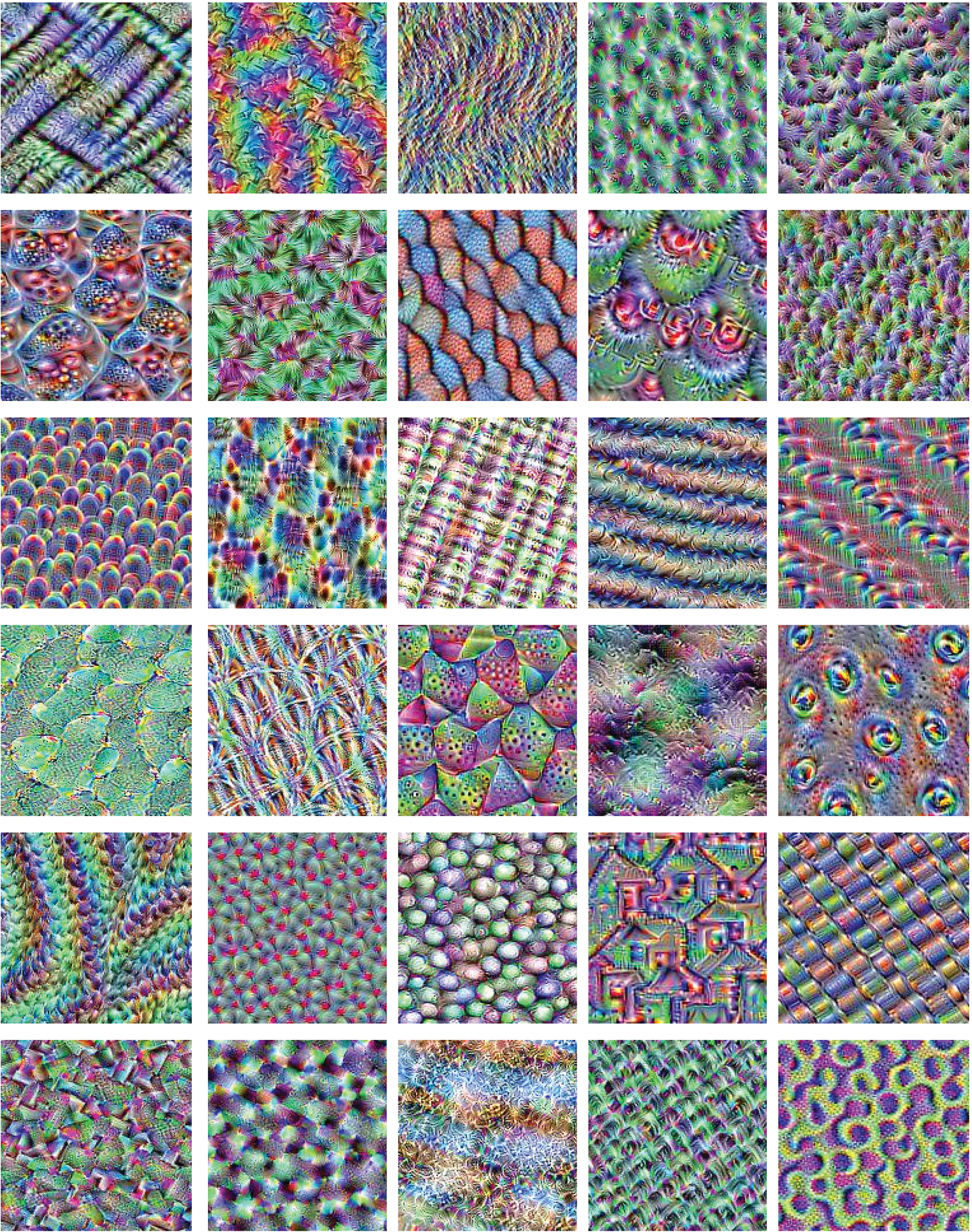
Figure 7: Some examples of artificial textures of BigTex
The image generation loop of step 2 has several parameters, and adjusting these parameters will result in changes to both the quality of the results and the processing speed. In this section, the parameters of this loop are discussed.
3.4.1 Selection Kernel for Texture Production
Each of the kernels in a pre-trained network is most sensitive to a specific pattern, which is extracted in step 2. The image patterns extracted by the kernels of the first layers contain general information and features, so the textures generated by these kernels often only contain color information or fine textures. These patterns are nearly identical across all networks. In addition, kernels from nearby layers extract similar features, so there is no need to utilize all network kernels. The kernels close to the output extract specific and more complex textures. Therefore, in this study, most of the selected kernels belong to the last layers (near the output) with a sufficient distance.
In step 2 of the proposed method, the ascending gradient loop is repeated 100 times. The texture result will also change when the repetition rate is altered. Table 4 shows some examples of these textures based on the number of loop repetitions. Based on this table, the more repetitions of the loop, the better and more complete textures are generated. In addition, many repetitions of the loop do not yield significant changes to the image. Therefore, this study considers the number of repetitions to be 100.
The learning rate of the loop should be selected in the proper range to generate appropriate images. If this value is chosen too small, the appropriate textures will not be generated, and most of the textures have blurred edges, which requires many repetition loops to solve this problem. If the learning rate is too high, it is possible that the loop does not converge and cannot generate proper texture. This value is set to 0.01.
3.4.4 Initial Values of the Input Image
The initial values of the image are randomly selected in the range near zero. Based on the implemented parts, the initial values of the input image have a minimal effect on the final result; however, it is advisable to set these values to small, near-zero values.
The initial dimension of the input image is 300 × 300 × 3. A value of 3 is to produce three color channels. The generated images are 300 × 300, which will be reduced during the following steps to remove margin points, often of lower quality than the rest of the image. Based on Table 4, the margin points of the generated textures include lower quality and blurred pixels. Therefore, at the end of the algorithm, 25 points are removed from each margin of the generated texture, resulting in a final dimension of 250 × 250.
Once again, in step 4, after applying image augmentation to increase the number of textures, the size of these textures is decreased. This is because applying image processing operations, such as shift, rotation, and zoom, created inappropriate margins that must be removed. Some of these examples are illustrated in Fig. 6. Therefore, 50 points are removed from each side of the textures, and the middle points of the 150 × 150 image are selected as the final image.
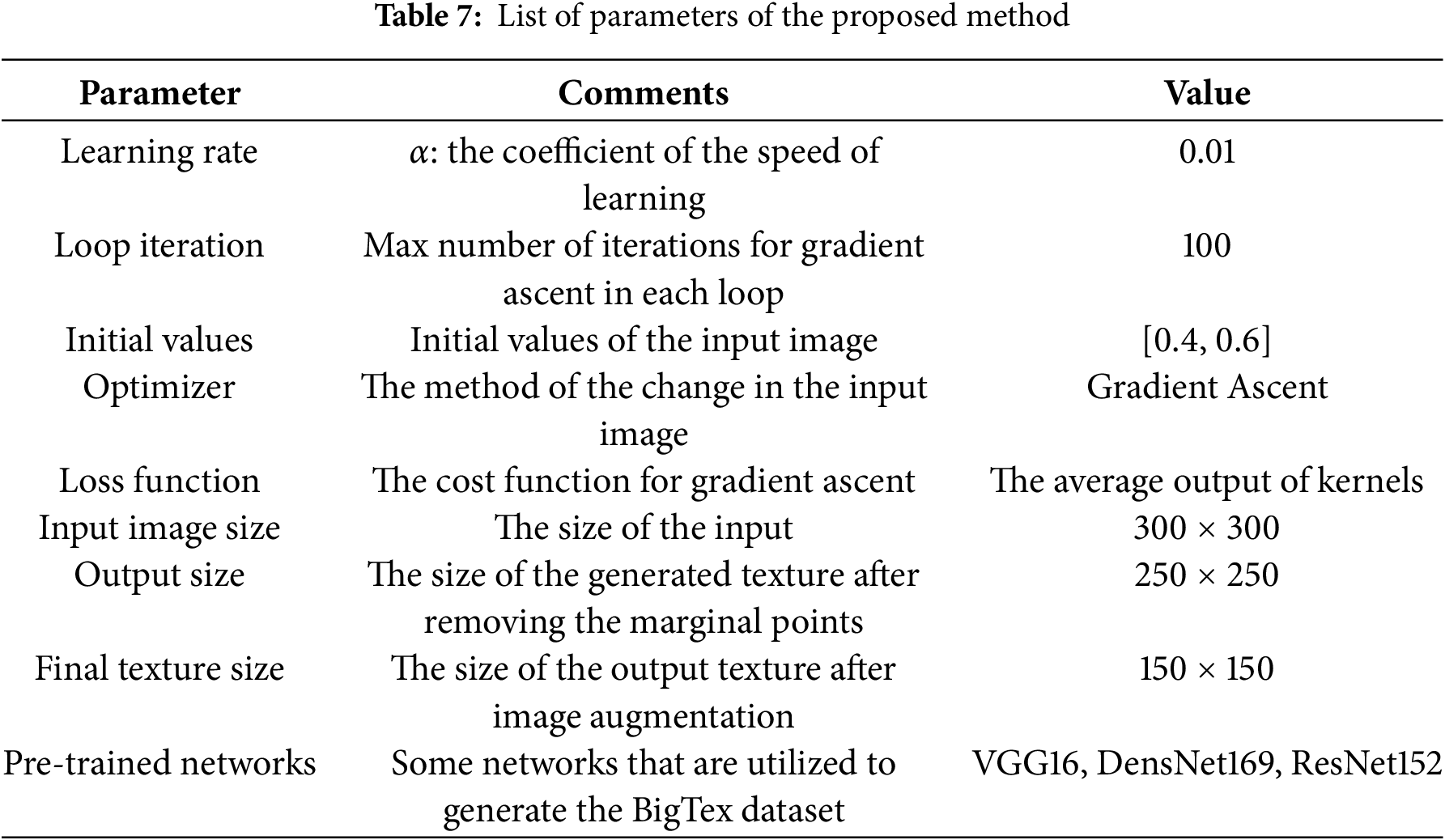
The loss function in the second step is the average of the output points of each convolution kernel. It should be maximized to generate the texture of each image. The gradient ascent increases this value in each step of the loop. When the output is maximized, the current image is used as a generated texture. In other words, each texture image generated from each kernel shows the highest sensitivity of that kernel to that image. Table 7 presents the list of all parameters for the proposed method, along with their values and explanations.
3.4.7 Image Augmentation and Its Parameters
This study uses only image augmentation to increase the number of textures for each class. In other words, it does not contribute to the generation of the new texture. Data augmentation possesses some desirable properties in most datasets. Generalization: Enables models to generalize effectively on unseen data. Efficiency of Data: Reduces the need for large annotated datasets. Minimization of Bias: Reduces overfitting to training artifacts. Robustness: Trained models using augmentations are robust against noise, occlusions, and mild distortions. Over-augmentation can harm performance if transformations render the image unrecognizable or alter the label’s meaning.
Table 6 indicates that some properties of the images are altered to reproduce them and increase the number. Horizontal move, vertical move, rotation, shear, zoom, horizontal flip, and brightness are some of these properties that are changed for texture augmentation in the proposed method. These properties and their values are only an example of changing the properties of texture images. Some other properties are not used for the image augmentation. Some of these include color, vertical flip, viewpoint, contrast, and illumination. These methods can be used for image augmentation as part of the proposed framework. However, some other image augmentation methods should not be used in this method. This is because these methods are not suitable for the texture and have a destructive effect on its properties. Some of these methods are image fusion, elastic transform, adding noise, and random erasing.
In terms of the value of each change in the texture property for augmentation, some properties, such as rotation, can be done with any value. However, for other properties, increasing the value of each change can remove most of the texture information, causing a large empty margin in the new images. Another important point for image augmentation is related to the features that can be extracted and their applications. For example, some local descriptors, such as the GLCM (gray level co-occurrence matrix) [84], are sensitive to illumination and rotation. In other words, the change in illumination and rotation for augmentation causes some challenges for clustering or classification by using GLCM features. Some other texture descriptors, such as LBP (local binary pattern), provide rotation-invariant and illumination-invariant features from each texture. In other words, rotation and illumination do not pose any challenge for these descriptors. LBP is not a scale-invariant descriptor; therefore, image augmentation by changing the zoom property poses a challenge for clustering or classification using LBP features.
3.5 Detect Incomplete and Similar Textures by Clustering
This section discusses some analysis methods for implementing texture detection to identify similar and incomplete textures. Several clustering methods can be employed for anomaly detection. If incomplete textures are assumed to be an anomaly in textures. It is possible to use some clustering, such as DBScan, to detect them. The first challenge for this issue is related to the feature vector of each texture. A large number of texture descriptors [87,88] are available for feature extraction from textures. Based on most previous research [89–91], some advanced local binary pattern methods (LBP) can extract more discriminative features from textures. CLBP is one of these methods. Table 8 presents the clustering results for detecting incomplete and similar textures using the CLBP feature vector. For similar texture, the results depend on several parameters, including the feature vectors, the number of clusters, the threshold value used for similarity, and the distance metric. In addition, the results can change significantly by adjusting the initial centers in specific methods, such as k-means.
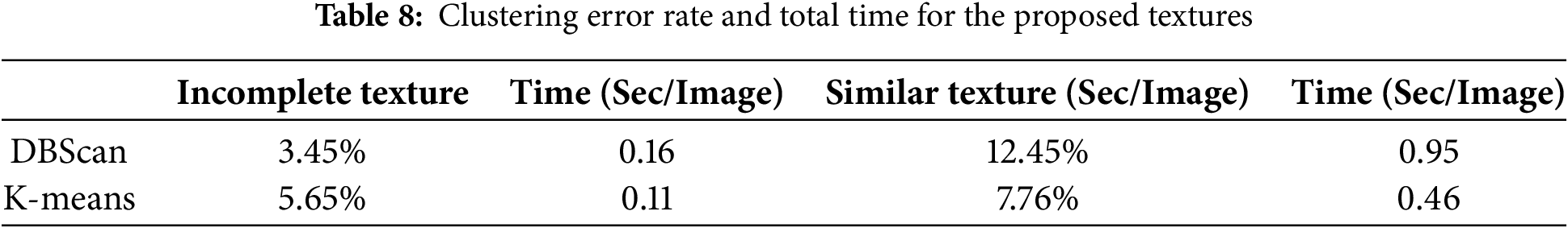
Table 8 indicates that using the clustering method to detect incomplete textures provides an acceptable error compared to the proposed method in step 3-2. However, for similar texture detection, the semi-automatic proposed method (steps 3-3) provides better error rates than clustering methods. This is because some textures have similar feature vectors, despite being visually different. Any change in the feature descriptor significantly alters the clustering results. If the semi-automatic or manual results are used as the benchmark, the error rate for similar textures reveals the difference between the manual results and the semi-automatic or manual results.
An artificial texture dataset called BigTex is generated from DensNet169, VGG16, and ResNet152 kernels, which contains 600 classes and 50 images per class.
Initially, 1000 new classes of texture were generated with the proposed method to create this dataset. Then, some similar and incomplete textures are removed. Finally, 600 texture classes were selected for image augmentation. Then, by using the common change in the image described in Table 6. Around 50 images were generated from each texture by using image augmentation and saved into each class. This dataset contains 30,000 color texture images with a size of 150 × 150. The size of its compressed file is around 2 GB.
4.1 Comparison to the Largest Texture Datasets
Table 9 lists the most famous and largest texture datasets. CUReT [92], Outex [93], Stex [94], and UIUC [95] are among the most well-known texture datasets. Brodatz [96] and MeasTex [97] are two other texture datasets that have been widely used in scientific studies over the past two decades. The largest texture dataset used in scientific papers is ALOT [98], which comprises 27,500 texture images across 250 classes. In terms of the most extensive variety of classes, the STex dataset has the largest number of texture classes, with 476 classes. Most of these data have no color and are single-channel or grayscale images.Trunk12 [99] and Virus [100] are two datasets with the highest and lowest resolution in this table.
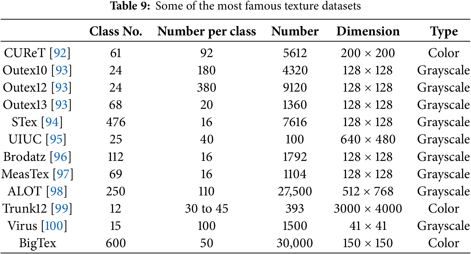
Table 9 indicates that almost all existing texture datasets cannot be classified as part of the big datasets. The dataset generated in this study (BigTex) is a color texture that utilizes only certain kernels from specific layers of the VGG, DenseNet, and ResNet networks. If kernels from other networks are employed, more classes can be generated, allowing for the creation of larger datasets. The number of images in each class increases by 50 times (50 images per class) through image processing for image augmentation. It is possible to increase this number to any desired number and create a bigger texture dataset.
4.2 Comparison of Image Quality
This section presents visual comparisons between the proposed method and some well-known methods. In generative networks, similar images are generated using original images. These methods are very time-consuming, and in most cases, the generated images have lower quality than the original images. Fig. 8 illustrates some examples of a visual comparison between texture images generated in the BigTex dataset and those generated using a generative network [101,102]. The quality of the textures produced by the proposed method is significantly better than that of generative methods. In addition, as mentioned earlier, the new texture class is generated using the proposed method. However, the generative networks produce images that are similar to the original textures. Most generative networks do not create a new texture class. The generative networks provide texture images from the original texture [102], which, in most cases, have many differences from the initial image and cannot be considered a new texture.
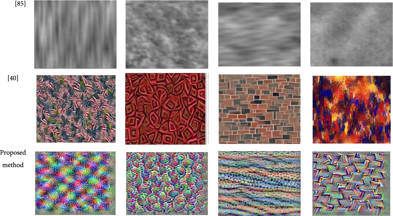
Figure 8: Comparison of images produced by the proposed method and some other methods
A visual comparison between the generated textures and some other methods is illustrated in Fig. 8. In some papers, several image quality metrics have been utilized to measure the clarity and quality of images. These metrics are divided into two groups: referenced and non-referenced metrics. The first group of metrics is employed to compare generated or output images with the original images. In other words, they used referenced or original images to estimate the quality of generated images. Some of these metrics include MSE (Mean Square Error), PSNR (Peak Signal-to-Noise Ratio), SSIM (Structural Similarity Index Measure) [103], correlation, and STSIM (Structural Texture Similarity Index Measure) [104]. The second metric is a reference-less metric that estimates the quality of generated images without any original images. Some of these criteria are G (Gradient) [105], Entropy [106], PIQE (Perception-based Image Quality Evaluator) [107], NIQE (Naturalness Image Quality Evaluator) [108], and BRISQUE (Blind/Referenceless Image Spatial Quality Evaluator) [109].
This study employs a proposed method to generate textures without relying on original images. Therefore, it is necessary to use either referenced or non-referenced metrics for comparing the generated textures to other texture images. Figs. 9 and 10 illustrate a comparison of the generated textures from the proposed method with other textures. Entropy and Gradient criteria are positive metrics, and PIQE, NIQE, and BRISQUE are negative metrics. In other words, in positive metrics, the greater the metric value, the better the result, and in negative metrics, the lower the metric value, the better the result. The BRISQUE and NIQE algorithms assess the quality score of an image with high computational efficiency once the model is trained. In contrast, PIQE provides local quality assessments alongside a global quality score. The gradient of an image represents a directional change in its intensity or color.
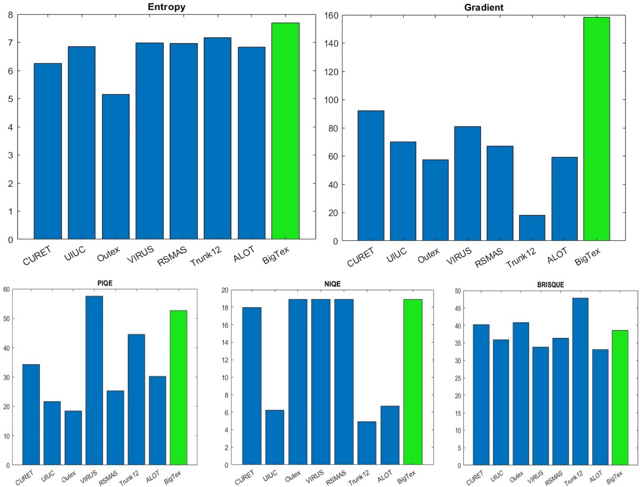
Figure 9: Comparing the quality of textures of the proposed method and some well-known texture datasets
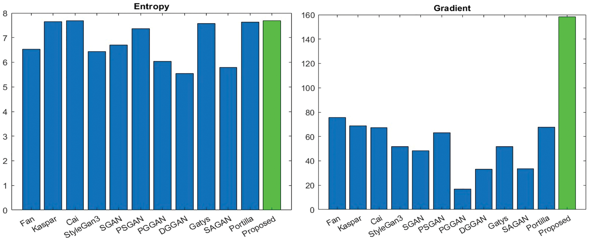
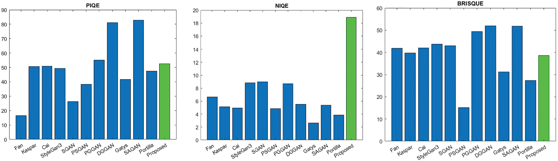
Figure 10: Comparing the quality of generated textures of the proposed and some other methods
Gradient [105] indicates the local details and information of the image. The higher the gradient, the better the image quality. The entropy, or average information, of an image can be determined approximately from its histogram. The histogram shows the different grey-level probabilities in the image. The higher entropy indicates a better quality of the image. It can be used for specific applications, such as autofocusing images [106].
PIQE integrates two fundamental aspects of the human visual system: background illumination and spatial frequency. These elements are essential for the precise assessment of image quality [110]. It estimates the quality of each image in the range of [0, 100] by calculating image distortion. NIQE is another image quality metric based on natural models. It is calculated in the range [0, inf) and it illustrates the naturalness of the image through the analysis of its statistical characteristics. NIQE is used when reference images are not accessible, and it can be applied to medical imaging and real-time applications. It is computed from images of natural scenes. A smaller score indicates better perceptual quality [111].
PIQE is inversely correlated to the perceptual quality of an image. The low value of PIQE indicates high perceptual quality, while the high value indicates low perceptual quality.
BRISQUE is another quality metric of image in the range [0, 100], and it relies on the natural scene statistics inherent in images. It concentrates on the spatial domain to determine image quality. A BRISQUE model is trained to estimate the quality of images with the same type of distortion [112]. The NIQE metric cannot correlate with human perception of quality as much as the BRISQUE metric. All of the PIQE, NIQE, and BRISQUE have a negative aspect. In other words, the lower the value for each of these metrics, the better the image quality.
Fig. 9 illustrates that the proposed method generates textures of higher quality, as assessed by both the Gradient and Entropy criteria. The average values of the gradient and entropy for all textures in each dataset are estimated. CUReT textures include very similar classes of textures. Outex is one of the most usable textures in most of the papers. UIUC is a dataset with very high details and sharp edges. The virus dataset includes small and low-resolution textures. Despite the Virus, the Trunk12 dataset includes high-resolution textures. RSMAS is a special texture dataset of Coral reefs, and ALOT is one of the largest available texture datasets. Fig. 9 indicates that, in terms of Entropy, the proposed method generates better textures with higher entropy than all other textures. In terms of the Gradient, the proposed method provides the textures with higher gradients or local details than other textures.
Fig. 9 shows some negative metrics (PIQE, NIQE, and BRISQUE) for comparing the quality of the textures. It indicates that the proposed method generates good textures; however, the quality of some other datasets is better than that of the proposed method. It illustrates that for the PIQE criteria, BigTex only provides better textures than Virus textures. In terms of the NIQE metric, the BigTex textures have the same quality as those of CURET, Outex, Virus, and RSMAS. However, the quality of UIUC, ALOT, and Trunk12 is better than that of the proposed textures.
Table 9 lists textures using the proposed method. Fig. 9 indicates that, for the BRISQUE metric, the proposed method generates a quality similar to that of some well-known datasets, such as CUReT and Outex. This criterion is high for huge textures such as Trunk12. Other textures, such as UIUC, Virus, RSMAS, and ALOT, provide better BRISQUE than BigTex.
Fig. 9 compares the quality of BigTex to that of different well-known texture datasets. Fig. 10 compares the quality of generated textures to some textures generated by some state-of-the-art GAN methods such as Fan et al. [49], Kapar [52], Cai et al. [113], StyleGan3 [114], sketch GAN (SGAN) [115], Periodic Spatial GAN (PSGAN) [40], Progressively Growing Generative Adversarial Network (PGGAN) [101], Deep Convolutional Generative Adversarial Network (DCGAN) [43], Gatys et al. [102] and Spatially Assembled Generative Adversarial Network (SAGAN) [44]. It also compares the results to a well-known parametric method, such as the method described in [41]. This figure shows that the proposed method provides significantly higher quality textures than all other methods, as measured by the Gradient metric. In addition, the proposed textures exhibit higher quality than other textures, as measured by the Entropy metric. Despite these two metrics, BigTex has lower quality than all other datasets according to the NIQE criterion. This is because this metric depends on the sizes of the textures, and the proposed textures have smaller sizes than other textures. As mentioned before, it is possible to enhance the quality of the generated textures by increasing the size of the output textures. Fig. 10 indicates that, by using the PIQE metric, the proposed method generates texture that is significantly better than that of DGGAN (Depth-image Guided Generative Adversarial Networks) and SAGAN. In addition, it performs slightly better than PGGAN. For the BRISQUE metric, the quality of the proposed textures is better than that of all other textures, except for the Potilla and Gytes methods.
Fig. 10 indicates that the proposed textures exhibit high distortion due to their low PIQE value. However, the NIQE metric value for the proposed textures indicates that they have a lower natural quality. This is due to the artificial textures generated by the proposed method.
4.4 Comparison of Processing Time
One of the significant challenges of processing in deep networks is the issue of training time, memory, and processor limitations. There are different methods to overcome this limitation. One of these methods is related to the use of pre-trained networks. In the proposed method, the training phase is omitted because a pre-trained network is used. The primary component of the proposed method’s processing time is the loop in the second step of Table 2, which takes approximately 2.3 s to generate the initial images of the second step, each with dimensions of 300 × 300, across 100 repetitions. Then, during the next step, incomplete textures are removed, and the margins around the generated images are cut after the data augmentation to create 150 × 150 images. For each image, the next two steps of the proposed method also require less than 1 s. Therefore, the average time to generate a texture is about 3.3 s. Table 9 presents a comparison of the time required to generate a texture image using the proposed method with the corresponding times in several generating networks. One of these methods for texture production is PGGAN [101]. The average processing time required for an image in the proposed method is much less than in the generative method. Google Colab is used in the proposed method for processing. Powerful hardware, including two Xenon 6138 20C 2.0 GHz processors with 192 GB of memory and two NVIDIA Tesla V100 graphics processors, is used in the PGGAN method [101]. In this method, 5 days are spent producing 1000 images with dimensions of 1024 × 1024, i.e., on average, 433 s are spent generating each texture.
A comparison of the processing time of some methods is listed in Table 10. This study must compare the processing time based on the dimensions of the output images. In this case, the proposed method requires approximately 94 s for each image with dimensions of 1024 × 1024, which is around 5 times faster than the PGGAN method. In addition, the hardware and processor used in the PGGAN method are significantly more powerful than those available on the free Google Colab.
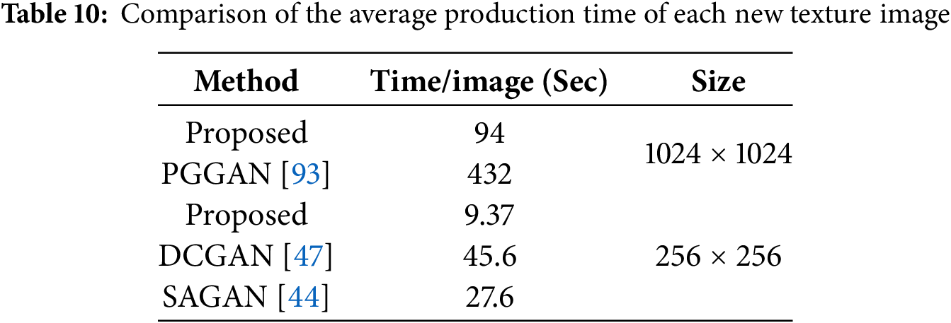
Table 10 details the time of two other well-known GAN methods for image generation [47]. Based on this table, the two methods, DCGAN [47] and SAGAN [48], require 45.6 and 27.6 s, respectively, to generate 256 × 256 textures. The proposed method generated each texture with this dimension in 9.37 s. This time is around 3 and 5 times faster than SAGAN and DCGAN, respectively.
4.5 Explanations about Quality Metrics and Computational Cost
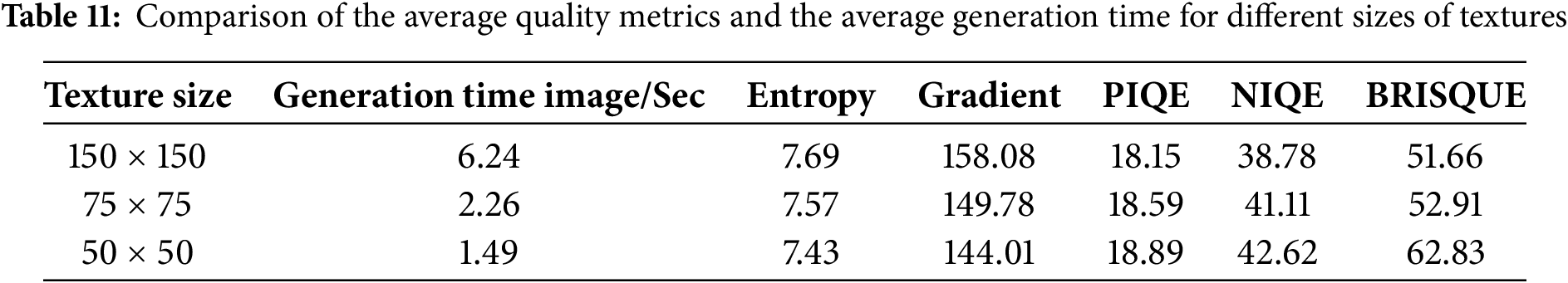
Table 11 presents the trade-offs between the quality of the generated textures of BigTex and the computational time required for each texture. This table indicates that for some quality metrics, such as PIQE and Entropy, the quality of textures slightly decreases when their size is decreased. However, for some other metrics, such as Gradient, this change is significant. In terms of the relationship between computational time and texture size, when the number of pixels is reduced to 1/4, the computation time decreases by approximately 1/3. This is because some operations are fixed and are performed every time, and they are not dependent on the size of the output textures.
4.6 Distinction Evaluation of the Generated Textures and Some Existing Textures
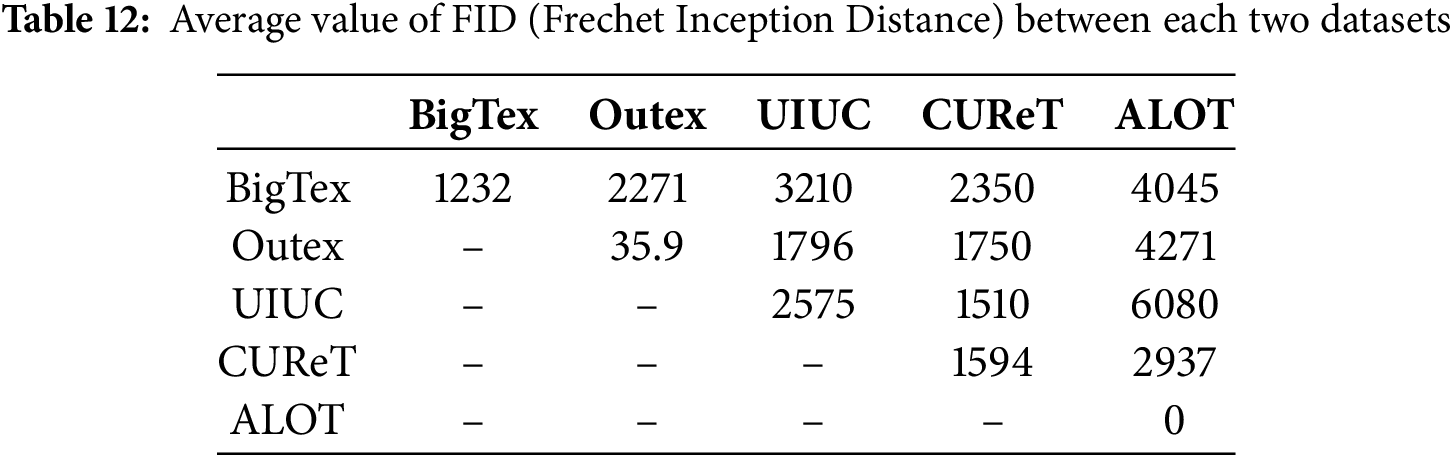
Fréchet inception distance (FID) [116] is a metric for quantifying the realism and diversity of images generated artificially. It is a special metric for evaluating the quality of images generated by models such as GANs. It measures the distance between two distributions, one from real images and one from generated images. It is estimated by comparing the mean and covariance of the features extracted. Relation 6 shows this metric. It includes the mean and covariance of the real and generated images. In addition, Tr is the trace operator, which calculates the sum of the diagonal elements.
FID is a positive value. However, it can be calculated as a minimal negative value. In this state, it must be set to zero. In this section, this metric is employed to distinguish the generated textures from various natural texture datasets. Table 12 indicates this metric for the proposed textures and some well-known textures. In terms of the FID criterion, the ALOT textures are more similar to each other because they have the lowest FID value. This metric for ALOT is a small negative value, and as mentioned in FID [116], when this value is small and negative, it should be set to zero. This metric indicates that the highest distinction lies between the ALOT and the UIUC textures. The BigTex artificial textures have enough distinction from other natural textures.
4.7 Evaluation of the Features of Textures by Feature Extraction and Classification
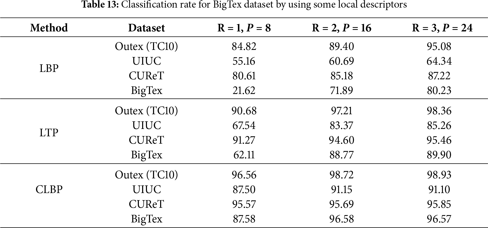
This section utilizes local descriptors to extract texture features, which are then used for classification. The classification results indicate that the generated textures include discriminative features, which can provide a high classification rate. In all datasets, half of the images for each class are used for training, and the remaining images are used for testing. K-NN with k = 1 is used for classification. In each method, the features of texture are extracted using LBP, Local Ternary Patterns (LTP) [117], and CLBP (LBP_S/M/C) [89] for three different neighborhood sizes. These methods employed the riu2 mapping [80] (relation 3). These results indicate the classification rate for the LBP features. These descriptors are rotation-invariant and illumination-invariant. However, they are not scale-invariant. Therefore, for BigTex textures that used zoom operation for image augmentation, LBP descriptors cannot extract robust features, especially for small neighborhoods. LTP is an LBP version that provides the noise-robust features. CLBP combines LBP (LBP_S), LBP_M (magnitude), and LBP_C (LBP center) and provides more discriminative features. Table 13 indicates these results.
4.8 Pre-Trained Networks: The Limitations and Advantages of the Proposed Method
Pre-trained networks have been developed for various purposes [83], such as decreasing the training computational time and processing burden. However, it includes some limitations, such as different types of pre-trained data and new data, input and output constraints, and accessibility restrictions.
This study utilizes the pre-trained networks proposed in the following section, which have both advantages and disadvantages. The main advantage of using these networks is that they can generate new texture classes without requiring high-complexity and large deep neural networks. In other words, it is possible to generate a new class of texture without powerful GPU units and high computational operations. Another advantage of the proposed method is that it generates new classes of texture that did not exist before. In other words, despite the GAN methods that generate new images similar to the input images, the proposed method can generate new texture classes without using any input textures.
In contrast, the proposed method includes some limitations. For example, the generated textures are produced artificially and cannot include all natural properties. The proposed method includes some semi-automatic steps that can be improved to make it fully automatic. In addition, the proposed method only utilizes pre-trained networks that were trained on ImageNet. This is due to the limitation of accessing other pre-trained networks. In other words, the pre-trained models used can have biases based on the original training dataset. Another limitation that can be addressed in future work is related to generating specific textures with specific properties. In other words, design an interpretable framework to generate textures specifically.
This research proposes a fast method based on convolution kernels and pre-trained networks to generate new texture images. Unlike the generative networks, the proposed method does not require initial images because it utilizes the same convolution coefficients as those calculated by the pre-trained network. In addition, unlike generative networks, this method has a significantly higher speed and does not require intensive processing. The primary motivation of the proposed method is to generate a new class of textures without relying on original textures.
The proposed algorithm consists of two manual and semi-automatic parts. It is possible to use specific techniques to automate these steps. For example, to delete similar textures, a stricter threshold can be used. However, it can remove some different textures. A more effective solution involves the use of advanced LBP versions [89,118,119] that yield more discriminative feature vectors for texture comparisons. Another solution is to use clustering methods to find similar textures and remove them. However, using these methods increases the computational cost of the algorithm.
Comparing the quality metrics for different texture datasets and generative texture methods reveals that, in terms of the Gradient and Entropy metrics, the proposed texture has better quality than all other datasets and models. The proposed method can be utilized to generate a bigger dataset by generating more than 50 images per class through image augmentation. In addition to avoiding data leakage, it is possible to increase the number of textures for each class by using more than one new texture.
The proposed method utilizes pre-trained networks that were trained on ImageNet. This is because only these networks are accessible at this time. The proposed method can be applied to any pre-trained network trained on various types of data. In other words, it is possible to generate various textures based on the initial training data.
One of the important points that can be addressed in the future is improving the quality of the generated textures for practical applications. One of the most important suggestions for future research is the provision of texture maps, for example, for printing on fabrics, carpets, and the weaving industry. The output of these textures is artificial and unlimited. In addition, some clustering methods, such as single-link clustering, can detect incomplete and similar textures from other textures. However, it drastically increases the computational complexity of texture generation.
Acknowledgement: This study is supported via funding from Prince Sattam bin Abdulaziz University project number (PSAU/2025/R/1446). Princess Nourah bint Abdulrahman University Researchers Supporting Project number (PNURSP2025R300). The authors would like to thank Prince Sultan University for their support.
Funding Statement: This study is supported via funding from Prince Sattam bin Abdulaziz University (PSAU/2025/R/1446), Princess Nourah bint Abdulrahman University (PNURSP2025R300), and Prince Sultan University.
Author Contributions: The authors confirm contribution to the paper as follows: Conceptualization, Farhan A. Alenizi and Faten Khalid Karim; methodology, Mohammad Hossein Shakoor; software, Farhan A. Alenizi; validation, Farhan A. Alenizi, Alaa R. Al-Shamasneh and Faten Khalid Karim; formal analysis, Mohammad Hossein Shakoor; investigation, Farhan A. Alenizi; resources, Mohammad Hossein Shakoor; data curation, Alaa R. Al-Shamasneh; writing—original draft preparation, Mohammad Hossein Shakoor; writing—review and editing, Faten Khalid Karim; visualization, Alaa R. Al-Shamasneh; supervision, Mohammad Hossein Shakoor; project administration, Faten Khalid Karim; funding acquisition, Farhan A. Alenizi and Faten Khalid Karim. All authors reviewed the results and approved the final version of the manuscript.
Availability of Data and Materials: Publicly available BigTex dataset here: https://drive.google.com/file/d/19z-QYSEGSMJOZ5Tr5p0EDIm55afbwVPU/view?usp=sharing (accessed on 20 July 2025).
Ethics Approval: Not applicable.
Conflicts of Interest: The authors declare no conflicts of interest to report regarding the present study.
Abbreviations
| IDC | International Data Corporation |
| GAN | Generative Adversarial Network |
| ZB | Zeta Byte |
| LBP | Local Binary Pattern |
| CLBP | Complete Local Binary Pattern |
| VGG | Visual Geometry Group |
| U | Uniform |
| TMP-GAN | Texture-constrained Multichannel Progressive Generative Adversarial Network |
| YOLO | You Only Look Once |
| CGAN | Conditional Generative Adversarial Network |
| SAGAN | Spatially Assembled Generative Adversarial Network |
| SGAN | Spatial Generative Adversarial Network |
| DCGAN | Deep Convolutional Generative Adversarial Network |
| PGGAN | Progressively Growing Generative Adversarial Network |
| MSE | Mean Square Error |
| PSNR | Peak Signal-to-Noise Ratio |
| SSIM | Structural Similarity Index Measure |
| STSIM | Structural Texture Similarity Index Measure |
| SPA | Self-Paced Augmentation |
| G | Gradient |
| PIQE | Perception-based Image Quality Evaluator |
| NIQE | Naturalness Image Quality Evaluator |
| BRISQUE | Blind/Referenceless Image Spatial Quality Evaluator |
References
1. Bin Inqiad W, Javed MF, Siddique MS, Alarifi SS, Alabduljabbar H. A comparative analysis of boosting and genetic programming techniques for predicting mechanical properties of soilcrete materials. Mater Today Commun. 2024;40(10):109920. doi:10.1016/j.mtcomm.2024.109920. [Google Scholar] [CrossRef]
2. Ala’a R, Al-Shamasneh R, Mahmoodzadeh NG, El Ouni MH. Forecasting mechanical properties of soilcrete enhanced with metakaolin employing diverse machine learning algorithms. Geomech Eng. 2025;40(2):123–37. doi:10.12989/gae.2025.40.2.123. [Google Scholar] [CrossRef]
3. Inqiad WB, Khan MS, Mehmood Z, Khan NM, Bilal M, Sazid M, et al. Utilizing contemporary machine learning techniques for determining soilcrete properties. Earth Sci Inform. 2025;18(1):176. doi:10.1007/s12145-024-01520-2. [Google Scholar] [CrossRef]
4. Hemdan EE, Al-Atroush ME. An efficient IoT-based soil image recognition system using hybrid deep learning for smart geotechnical and geological engineering applications. Multimed Tools Appl. 2024;83(25):66591–612. doi:10.1007/s11042-024-18230-y. [Google Scholar] [CrossRef]
5. McAfee A, Brynjolfsson E, Davenport TH, Patil DJ, Barton D. Big data: the management revolu-tion. Harv Bus Rev. 2012;90(10):60–8. [Google Scholar] [PubMed]
6. Kune R, Konugurthi PK, Agarwal A, Chillarige RR, Buyya R. The anatomy of big data computing. Softw Pract Exp. 2016;46(1):79–105. doi:10.1002/spe.2374. [Google Scholar] [CrossRef]
7. Fu Y, Li X, Ye Y. A multi-task learning model with adversarial data augmentation for classification of fine-grained images. Neurocomputing. 2020;377(10):122–9. doi:10.1016/j.neucom.2019.10.002. [Google Scholar] [CrossRef]
8. Xu M, Yoon S, Fuentes A, Park DS. A comprehensive survey of image augmentation techniques for deep learning. Pattern Recognit. 2023;137(1):109347. doi:10.1016/j.patcog.2023.109347. [Google Scholar] [CrossRef]
9. Di Cataldo S, Ficarra E. Mining textural knowledge in biological images: applications, methods and trends. Comput Struct Biotechnol J. 2017;15(7):56–67. doi:10.1016/j.csbj.2016.11.002. [Google Scholar] [PubMed] [CrossRef]
10. Srivastava N, Hinton G, Krizhevsky A, Sutskever I, Salakhutdinov R. Dropout: a simple way to prevent neural networks from overfitting. J Mach Learn Res. 2014;15:1929–58. [Google Scholar]
11. Selmy HA, Mohamed HK, Medhat W. Big data analytics deep learning techniques and applications: a survey. Inf Syst. 2024;120:102318. doi:10.1016/j.is.2023.102318. [Google Scholar] [CrossRef]
12. Wang J, Perez L. The effectiveness of data augmentation in image classification using deep learning. Convolutional Neural Netw Vis Recognit. 2017;11(2017):1–8. [Google Scholar]
13. Tosi D, Kokaj R, Roccetti M. 15 years of big data: a systematic literature review. J Big Data. 2024;11(1):73. doi:10.1186/s40537-024-00914-9. [Google Scholar] [CrossRef]
14. Berloco F, Bevilacqua V, Colucci S. Distributed analytics for big data: a survey. Neurocomputing. 2024;574(1):127258. doi:10.1016/j.neucom.2024.127258. [Google Scholar] [CrossRef]
15. Shorten C, Khoshgoftaar TM. A survey on image data augmentation for deep learning. J Big Data. 2019;6(1):60. doi:10.1186/s40537-019-0197-0. [Google Scholar] [CrossRef]
16. Szegedy C, Vanhoucke V, Ioffe S, Shlens J, Wojna Z. Rethinking the inception architecture for computer vision. arXiv:1512.00567. 2015. [Google Scholar]
17. He K, Zhang X, Ren S, Sun J. Deep residual learning for image recognition. arXiv:1512.03385. 2016. [Google Scholar]
18. Huang G, Liu Z, van der Maaten L, Weinberger KQ. Densely connected convolutional networks. arXiv:1608.06993. 2016. [Google Scholar]
19. Krizhevsky A, Sutskever I, Hinton GE. ImageNet classification with deep convolutional neural networks. In: Advances in neural information processing systems. La Jolla, CA, USA: NIPS; 2012. 25 p. doi:10.1145/3065386. [Google Scholar] [CrossRef]
20. Redmon J, Divvala S, Girshick R, Farhadi A. You only look once: unified, real-time object de-tection. arXiv.1506.02640. 2016. [Google Scholar]
21. Wan D, Lu R, Xu T, Shen S, Lang X, Ren Z. Random Interpolation Resize: a free image data augmentation method for object detection in industry. Expert Syst Appl. 2023;228(24):120355. doi:10.1016/j.eswa.2023.120355. [Google Scholar] [CrossRef]
22. Takase T, Karakida R, Asoh H. Self-paced data augmentation for training neural networks. Neurocomputing. 2021;442(11):296–306. doi:10.1016/j.neucom.2021.02.080. [Google Scholar] [CrossRef]
23. Bochkovskiy A, Wang CY, Liao HYM. Yolov4: optimal speed and accuracy of object detection. arXiv:2004.10934. 2020. [Google Scholar]
24. Hendrycks D, Mu N, Cubuk ED, Zoph B, Gilmer J, Lakshminarayanan B. Augmix: a simple method to improve robustness and uncertainty under data shift. In: International Conference on Learning Representations; 2020 Apr 30; Addis Ababa, Ethiopia. [Google Scholar]
25. Dwibedi D, Misra I, Hebert M. Cut, paste and learn: surprisingly easy synthesis for instance detection. In: 2017 IEEE International Conference on Computer Vision (ICCV); 2017 Oct 22–29; Venice, Italy. p. 1310–9. doi:10.1109/iccv.2017.146. [Google Scholar] [CrossRef]
26. Ghiasi G, Cui Y, Srinivas A, Qian R, Lin TY, Cubuk ED et al. Simple copy-paste is a strong data augmentation method for instance segmentation. In: 2021 IEEE/CVF Conference on Computer Vision and Pattern Recognition (CVPR); 2021 Jun 20–25; Nashville, TN, USA. p. 2917–27. doi:10.1109/cvpr46437.2021.00294. [Google Scholar] [CrossRef]
27. Baek K, Bang D, Shim H. Gridmix: strong regularization through local context mapping. Pattern Recognit. 2021;109(1):107594. doi:10.1016/j.patcog.2020.107594. [Google Scholar] [CrossRef]
28. Li C, Wand M. Combining Markov random fields and convolutional neural networks for image synthesis. In: 2016 IEEE Conference on Computer Vision and Pattern Recognition (CVPR); 2016 Jun 27–30; Las Vegas, NV, USA. p. 2479–86. doi:10.1109/CVPR.2016.272. [Google Scholar] [CrossRef]
29. Efros AA, Freeman WT. Image quilting for texture synthesis and transfer. In: Proceedings of the 28th Annual Conference on Computer Graphics and Interactive Techniques; 2001 Aug 12–17; Los Angeles, CA, USA. p. 341–6. doi:10.1145/383259.383296. [Google Scholar] [CrossRef]
30. Wei L, Lefebvre S, Kwatra V, Turk G. State of the art in example-based texture synthesis. In: Eurographics 2009, state of the art report, EG-STAR. Eindhoven, The Netherlands: Eurographics Association; 2009. p. 93–117. [Google Scholar]
31. Julesz B. Visual pattern discrimination. IRE Trans Inf Theory. 1962;8(2):84–92. doi:10.1109/tit.1962.1057698. [Google Scholar] [CrossRef]
32. Portilla J, Simoncelli EP. A parametric texture model based on joint statistics of complex wavelet coefficients. Int J Comput Vis. 2000;40(1):49–70. [Google Scholar]
33. Kaspar A, Neubert B, Lischinski D, Pauly M, Kopf J. Self tuning texture optimization. Comput Graph Forum. 2015;34(2):349–59. doi:10.1111/cgf.12565. [Google Scholar] [CrossRef]
34. Qian W, Cao J, Xu D, Nie R, Guan Z. Synthesis of exemplar textures by self-similarity matching. J Electron Imaging. 2018;27(6):063034. doi:10.1117/1.JEI.27.6.063034. [Google Scholar] [CrossRef]
35. Dong X, Dong J, Sun G, Duan Y, Qi L, Yu H. Learning-based texture synthesis and automatic inpainting using support vector machines. IEEE Trans Ind Electron. 2019;66(6):4777–87. doi:10.1109/TIE.2018.2866043. [Google Scholar] [CrossRef]
36. Yang C, Liu Q, Wang C, Ding J, Cheung YM. Self-tuning transfer dynamic convolution autoencoder for quality prediction of multimode processes with shifts. IEEE Trans Ind Inform. 2024;20(9):11295–305. doi:10.1109/TII.2024.3399932. [Google Scholar] [CrossRef]
37. Goodfellow IJ, Pouget-Abadie J, Mirza M, Xu B, Warde-Farley D, Ozair S et al. Generative adversarial nets. In: Proceedings of the 28th International Conference on Neural Information Processing Systems, NIPS’14. Cambridge, MA, USA: MIT Press; 2014. p. 2672–80. [Google Scholar]
38. Mirza M, Osindero S. Conditional generative adversarial nets. arXiv:1411.1784. 2014. [Google Scholar]
39. Kim SE, Yoon H, Lee J. Fast and scalable earth texture synthesis using spatially assembled generative adversarial neural networks. J Contam Hydrol. 2021;243(4):103867. doi:10.1016/j.jconhyd.2021.103867. [Google Scholar] [PubMed] [CrossRef]
40. Bergmann U, Jetchev N, Vollgraf R. Learning texture manifolds with the periodic spatial GAN. In: Precup D, Teh YW, editors. Proceedings of the 34th International Conference on Machine Learning. Westminster, UK: PMLR; 2017. p. 469–77. [Google Scholar]
41. Li X, Mariethoz G, Lu D, Linde N. Patch-based iterative conditional geostatistical simulation using graph cuts. Water Resour Res. 2016;52(8):6297–320. doi:10.1002/2015wr018378. [Google Scholar] [CrossRef]
42. Guan Q, Chen Y, Wei Z, Heidari AA, Hu H, Yang XH, et al. Medical image augmentation for lesion detection using a texture-constrained multichannel progressive GAN. Comput Biol Med. 2022;145:105444. doi:10.1016/j.compbiomed.2022.105444. [Google Scholar] [PubMed] [CrossRef]
43. Zdunek R. Hybrid texture synthesis and interpolated structure image completion. Procedia Comput Sci. 2022;207:2464–73. doi:10.1016/j.procs.2022.09.304. [Google Scholar] [CrossRef]
44. Radford A, Metz L, Chintala S. Unsupervised representation learning with deep convolutional generative adversarial networks. arXiv:1511.06434. 2015. doi: 10.48550/arXiv.1511.06434. [Google Scholar] [CrossRef]
45. Jetchev N, Bergmann U, Vollgraf R. Texture synthesis with spatial generative adversarial networks. arXiv:1611.08207. 2016. [Google Scholar]
46. Fan J, Shi XY, Zhou Z, Tang Y. A fast texture-by-numbers synthesis method based on texture optimization. In: Proceedings of the 5th International Symposium on Visual Information Communication and Interaction; 2012 Sep 27–28; Hangzhou, China. p. 1–10. doi:10.1145/2397696.2397697. [Google Scholar] [CrossRef]
47. Abdellatif A, Elsheikh AH. Generating infinite-resolution texture using GANs with patch-by-patch paradigm. arXiv:2309.02340. 2023. [Google Scholar]
48. Salari E, Azimifar Z. Texture image synthesis using spatial GAN based on vision transformers. arXiv:2502.01842. 2025. [Google Scholar]
49. Fan W, Fang J, Huang G. An improved image texture synthesis based on algorithm convolution neural network. Phys Commun. 2024;66(5):102395. doi:10.1016/j.phycom.2024.102395. [Google Scholar] [CrossRef]
50. Paget R, Longstaff ID. Texture synthesis via a noncausal nonparametric multiscale Markov random field. IEEE Trans Image Process. 1998;7(6):925–31. doi:10.1109/83.679446. [Google Scholar] [PubMed] [CrossRef]
51. Efros AA, Leung TK. Texture synthesis by non-parametric sampling. In: Proceedings of the Seventh IEEE International Conference on Computer Vision; 1999 Sep 20–27; Kerkyra, Greece. p. 1033–8. doi:10.1109/ICCV.1999.790383. [Google Scholar] [CrossRef]
52. Erhan D, Bengio Y, Courville A, Manzagol PA, Vincent P. Why does unsupervised pre-training help deep learning? J Mach Learn Res. 2010;11:625–60. [Google Scholar]
53. Miguel JPM, Neves LA, Martins AS, do Nascimento MZ, Tosta TAA. Analysis of neural networks trained with evolutionary algorithms for the classification of breast cancer histological images. Expert Syst Appl. 2023;231(1):120609. doi:10.1016/j.eswa.2023.120609. [Google Scholar] [CrossRef]
54. Singh SA, Kumar AS, Desai KA. Comparative assessment of common pre-trained CNNs for vision-based surface defect detection of machined components. Expert Syst Appl. 2023;218(6):119623. doi:10.1016/j.eswa.2023.119623. [Google Scholar] [CrossRef]
55. Gowthamy J, Ramesh S. A novel hybrid model for lung and colon cancer detection using pre-trained deep learning and KELM. Expert Syst Appl. 2024;252(10):124114. doi:10.1016/j.eswa.2024.124114. [Google Scholar] [CrossRef]
56. Deng J, Dong W, Socher R, Li LJ, Li K, Li F. ImageNet: a large-scale hierarchical image dataset. In: 2009 IEEE Conference on Computer Vision and Pattern Recognition; 2009 Jun 20–25; Miami, FL, USA. p. 248–55. [Google Scholar]
57. Simonyan K, Zisserman A. Very deep convolutional networks for large-scale image recognition. arXiv:1409.1556. 2014. [Google Scholar]
58. Ojala T, Pietikäinen M, Harwood D. A comparative study of texture measures with classification based on featured distributions. Pattern Recognit. 1996;29(1):51–9. doi:10.1016/0031-3203(95)00067-4. [Google Scholar] [CrossRef]
59. Singh KK, Lee YJ. Hide-and-seek: forcing a network to be meticulous for weakly-supervised object and action localization. In: 2017 IEEE International Conference on Computer Vision (ICCV); 2017 Oct 22–29; Venice, Italy. p. 3544–53. doi:10.1109/ICCV.2017.381. [Google Scholar] [CrossRef]
60. Chen P, Liu S, Zhao H, Jia J. Grid mask data augmentation. arXiv:2001.04086. 2020. [Google Scholar]
61. DeVries T, Taylor GW. Improved regularization of convolutional neural networks with cutout. arXiv:1708.04552. 2017. [Google Scholar]
62. Zhong Z, Zheng L, Kang G, Li S, Yang Y. Random erasing data augmentation. Proc AAAI Conf Artif Intell. 2020;34(7):13001–8. doi:10.1609/aaai.v34i07.7000. [Google Scholar] [CrossRef]
63. Inoue H. Data augmentation by pairing samples for images classification. arXiv:1801.02929. 2018. [Google Scholar]
64. Yun S, Han D, Chun S, Oh SJ, Yoo Y, Choe J. CutMix: regularization strategy to train strong classifiers with localizable features. In: 2019 IEEE/CVF International Conference on Computer Vision (ICCV); 2019 Oct 27–Nov 2; Seoul, Republic of Korea. p. 6022–31. doi:10.1109/iccv.2019.00612. [Google Scholar] [CrossRef]
65. Zhang H, Cisse M, Dauphin YN, Lopez-Paz D. Mixup: beyond empirical risk minimization. arXiv:1710.09412. 2017. [Google Scholar]
66. Tokozume Y, Ushiku Y, Harada T. Between-class learning for image classification. In: 2018 IEEE/CVF Conference on Computer Vision and Pattern Recognition; 2018 Jun 18–23; Salt Lake City, UT, USA. p. 5486–94. doi:10.1109/CVPR.2018.00575. [Google Scholar] [CrossRef]
67. Moradi M, Madani A, Karargyris A, Syeda-Mahmood TF. Chest X-ray generation and data augmentation for cardiovascular abnormality classification. In: Medical Imaging 2018: Image Processing; 2018 Feb 10–15; Houston, TX, USA. doi:10.1117/12.2293971. [Google Scholar] [CrossRef]
68. Huang SW, Lin CT, Chen SP, Wu YY, Hsu PH, Lai SH. AugGAN: cross domain adaptation with GAN-based data augmentation. In: Computer vision–ECCV 2018. Cham, Switzerland: Springer International Publishing; 2018. p. 731–44. doi: 10.1007/978-3-030-01240-3_44. [Google Scholar] [CrossRef]
69. Zheng Z, Yu Z, Wu Y, Zheng H, Zheng B, Lee M. Generative Adversarial Network with Multi-branch Discriminator for imbalanced cross-species image-to-image translation. Neural Netw. 2021;141(1):355–71. doi:10.1016/j.neunet.2021.04.013. [Google Scholar] [PubMed] [CrossRef]
70. Zhu X, Liu Y, Li J, Wan T, Qin Z. Emotion classification with data augmentation using generative adversarial networks. In: Advances in knowledge discovery and data mining. Cham, Switzerland: Springer International Publishing; 2018. p. 349–60. doi: 10.1007/978-3-319-93040-4_28. [Google Scholar] [CrossRef]
71. Xiong X, Shen C, Wu J, Lü S, Zhang X. Combined data augmentation framework for generalizing deep reinforcement learning from pixels. Expert Syst Appl. 2025;264(2):125810. doi:10.1016/j.eswa.2024.125810. [Google Scholar] [CrossRef]
72. Lu Y, Chen D, Olaniyi E, Huang Y. Generative adversarial networks (GANs) for image augmentation in agriculture: a systematic review. Comput Electron Agric. 2022;200(7):107208. doi:10.1016/j.compag.2022.107208. [Google Scholar] [CrossRef]
73. Fawzi A, Samulowitz H, Turaga D, Frossard P. Adaptive data augmentation for image classification. In: 2016 IEEE International Conference on Image Processing (ICIP); 2016 Sep 25–28; Phoenix, AZ, USA. p. 3688–92. doi:10.1109/ICIP.2016.7533048. [Google Scholar] [CrossRef]
74. Ho D, Liang E, Chen X, Stoica I, Abbeel P. Population based augmentation: efficient learning of augmentation policy schedules. In: Proceedings of the 36th International Conference on Machine Learning; 2019 Jun 9–15; Long Beach, CA, USA. p. 2731–41. [Google Scholar]
75. Hataya R, Zdenek J, Yoshizoe K, Nakayama H. Meta approach to data augmentation optimization. In: 2022 IEEE/CVF Winter Conference on Applications of Computer Vision (WACV); 2022 Jan 3–8; Waikoloa, HI, USA. p. 3535–44. doi:10.1109/WACV51458.2022.00359. [Google Scholar] [CrossRef]
76. Hataya R, Zdenek J, Yoshizoe K, Nakayama H. Faster AutoAugment: learning augmentation strategies using backpropagation. In: Computer vision–ECCV 2020. Cham: Springer International Publishing; 2020. p. 1–16. doi: 10.1007/978-3-030-58595-2_1. [Google Scholar] [CrossRef]
77. Cubuk ED, Zoph B, Shlens J, Le QV. Randaugment: practical automated data augmentation with a reduced search space. In: 2020 IEEE/CVF Conference on Computer Vision and Pattern Recognition Workshops (CVPRW); 2020 Jun 14–19; Seattle, WA, USA. p. 3008–17. doi:10.1109/cvprw50498.2020.00359. [Google Scholar] [CrossRef]
78. Zoph B, Cubuk ED, Ghiasi G, Lin TY, Shlens J, Le QV. Learning data augmentation strategies for object detection. In: Computer Vision – ECCV 2020. Cham: Springer International Publishing; 2020. p. 566–83. doi: 10.1007/978-3-030-58583-9_34. [Google Scholar] [CrossRef]
79. Ratner AJ, Ehrenberg HR, Hussain Z, Dunnmon J, Ré C. Learning to compose domain-specific transformations for data augmentation. Adv Neural Inf Process Syst. 2017;30:3239–49. [Google Scholar] [PubMed]
80. Li P, Liu X, Xie X. Learning sample-specific policies for sequential image augmentation. In: Proceedings of the 29th ACM International Conference on Multimedia; 2021 Oct 20–24; Online. p. 4491–500. doi:10.1145/3474085.3475602. [Google Scholar] [CrossRef]
81. Tang Z, Peng X, Li T, Zhu Y, Metaxas D. AdaTransform: adaptive data transformation. In: 2019 IEEE/CVF International Conference on Computer Vision (ICCV); 2019 Oct 27–Nov 2; Seoul, Republic of Korea. p. 2998–3006. doi:10.1109/ICCV.2019.00309. [Google Scholar] [CrossRef]
82. Sun D, Dornaika F, Charafeddine J. LCAMix: local-and-contour aware grid mixing based data augmentation for medical image segmentation. Inf Fusion. 2024;110(1):102484. doi:10.1016/j.inffus.2024.102484. [Google Scholar] [CrossRef]
83. Chollet F. Deep learning with Python. Shelter Island, NY, USA: Manning; 2017. [Google Scholar]
84. Haralick RM, Shanmugam K, Dinstein I. Textural features for image classification. IEEE Trans Syst Man Cybern. 1973;SMC-3(6):610–21. doi:10.1109/TSMC.1973.4309314. [Google Scholar] [CrossRef]
85. Karanwal S, Diwakar M. OD-LBP: orthogonal difference-local binary pattern for Face Recognition. Digit Signal Process. 2021;110(10):102948. doi:10.1016/j.dsp.2020.102948. [Google Scholar] [CrossRef]
86. Tian G, Fu H, Dagan Feng D. Automatic medical image categorization and annotation using LBP and MPEG-7 edge histograms. In: 2008 International Conference on Information Technology and Applications in Biomedicine; 2008 May 30–31; Shenzhen, China. p. 51–3. doi:10.1109/ITAB.2008.4570523. [Google Scholar] [CrossRef]
87. Ojala T, Pietikainen M, Maenpaa T. Multiresolution gray-scale and rotation invariant texture classification with local binary patterns. IEEE Trans Pattern Anal Mach Intell. 2002;24(7):971–87. doi:10.1109/TPAMI.2002.1017623. [Google Scholar] [CrossRef]
88. Shakoor MH, Boostani R. Extended mapping local binary pattern operator for texture classification. Int J Patt Recogn Artif Intell. 2017;31(6):1750019. doi:10.1142/s0218001417500197. [Google Scholar] [CrossRef]
89. Guo Z, Zhang L, Zhang D. A completed modeling of local binary pattern operator for texture classification. IEEE Trans Image Process. 2010;19(6):1657–63. doi:10.1109/TIP.2010.2044957. [Google Scholar] [PubMed] [CrossRef]
90. Ramprasaath RS, Cogswell M, Das A, Vedantam R, Parikh D, Batra D. Grad-CAM: visual explanations from deep networks via gradient-based localization. arXiv:1610.02391. 2017. [Google Scholar]
91. Bianconi F, Fernández A. On the occurrence probability of local binary patterns: atheoretical study. J Math Imag Vis. 2011;40(3):259–68. doi:10.1007/s10851-011-0261-7. [Google Scholar] [CrossRef]
92. Dana KJ, van Ginneken B, Nayar SK, Koenderink JJ. Reflectance and texture of real-world surfaces. ACM Trans Graph. 1999;18(1):1–34. doi:10.1145/300776.300778. [Google Scholar] [CrossRef]
93. Ojala T, Mäenpää T, Pietikäinen M, Viertola J, Kyllönen J, Huovinen S. Outex—new framework for empirical evaluation of texture analysis algorithm. In: 2002 International Conference on Pattern Recognition; 2002 Aug 11–15; Quebec City, QC, Canada. p. 701–6. [Google Scholar]
94. Backes AR, Casanova D, Bruno OM. Color texture analysis based on fractal descriptors. Pattern Recognit. 2012;45(5):1984–92. doi:10.1016/j.patcog.2011.11.009. [Google Scholar] [CrossRef]
95. Lazebnik S, Schmid C, Ponce J. A sparse texture representation using local affine regions. IEEE Trans Pattern Anal Mach Intell. 2005;27(8):1265–78. doi:10.1109/TPAMI.2005.151. [Google Scholar] [PubMed] [CrossRef]
96. Brodatz P. Textures: a photographic album for artists and designers. New York, NY, USA: Dover Publications, 1966. doi:10.2307/1571915. [Google Scholar] [CrossRef]
97. Smith G. MeasTex image texture dataset and test suite centre for sensor signal and information processing. [Dataset]. Brisbane, QLD, Australia: The University of Queensland; 1998. [Google Scholar]
98. Burghouts GJ, Geusebroek JM. Material-specific adaptation of color invariant features. Pattern Recogn Lett. 2009;30(3):306–13. doi:10.1016/j.patrec.2008.10. [Google Scholar] [CrossRef]
99. Ratajczak R, Bertrand S, Crispim CJ, Tougne L. Efficient bark recognition in the wild. In: Proceedings of the 14th International Joint Conference on Computer Vision, Imaging and Computer Graphics Theory and Applications; 2019 Feb 25–27; Prague, Czech Republic. p. 240–8. [Google Scholar]
100. Kylberg G. Virus Texture Dataset V. 1.0. 2012 [Internet]. [cited 2025 Jul 20]. Available from: http://www.cb.uu.se/~gustaf/virustexture. [Google Scholar]
101. Eastwood J, Newton L, Leach R, Piano S. Generation and categorisation of surface texture data using a modified progressively growing adversarial network. Precis Eng. 2022;74:1–11. doi:10.1016/j.precisioneng.2021.10.020. [Google Scholar] [CrossRef]
102. Gatys A, Ecker AS, Bethge M. A neural algorithm of artistic style. arXiv:1508. 06576. 2015. [Google Scholar]
103. Wang Z, Bovik AC, Sheikh HR, Simoncelli EP. Image quality assessment: from error visibility to structural similarity. IEEE Trans Image Process. 2004;13(4):600–12. doi:10.1109/TIP.2003.819861. [Google Scholar] [PubMed] [CrossRef]
104. Zujovic J, Pappas TN, Neuhoff DL. Structural texture similarity metrics for image analysis and retrieval. IEEE Trans Image Process. 2013;22(7):2545–58. doi:10.1109/TIP.2013.2251645. [Google Scholar] [PubMed] [CrossRef]
105. Jacobs D. Image gradients. In: Class notes for CMSC 426. Ho Chi Minh City, Vietnam: HCMC University of Technology (HCMUT); 2005. [Google Scholar]
106. Ch T. Measurement of the entropy of an image with application to image focusing. Opt Acta Int J Opt. 1984;31(2):203–11. doi:10.1080/713821475. [Google Scholar] [CrossRef]
107. Venkatanath N, Praneeth D, Bh MC, Channappayya SS, Medasani SS. Blind image quality evaluation using perception based features. In: 2015 Twenty First National Conference on Communications (NCC); 2015 Feb 27–Mar 1; Mumbai, India. p. 1–6. doi:10.1109/NCC.2015.7084843. [Google Scholar] [CrossRef]
108. Mittal A, Soundararajan R, Bovik AC. Making a “completely blind” image quality analyzer. IEEE Signal Process Lett. 2013;20(3):209–12. doi:10.1109/LSP.2012.2227726. [Google Scholar] [CrossRef]
109. Mittal A, Moorthy AK, Bovik AC. No-reference image quality assessment in the spatial domain. IEEE Trans Image Process. 2012;21(12):4695–708. doi:10.1109/TIP.2012.2214050. [Google Scholar] [PubMed] [CrossRef]
110. Saghri JA, Cheatham PS, Habibi A. Image quality measure based on a human visual system model. Opt Eng. 1989;28(7):813–18. doi:10.1117/12.7977038. [Google Scholar] [CrossRef]
111. Kastryulin S, Zakirov J, Pezzotti N, Dylov DV. Image quality assessment for magnetic resonance imaging. IEEE Access. 2023;11(3):14154–68. doi:10.1109/access.2023.3243466. [Google Scholar] [CrossRef]
112. Callet PL, Barba D. A robust quality metric for color image quality assessment. In: Proceedings 2003 International Conference on Image Processing; 2003 Sep 14–17; Barcelona, Spain. p. 437–40. doi:10.1109/ICIP.2003.1246992. [Google Scholar] [CrossRef]
113. Cai X, Song B, Fang Z. Exemplar based regular texture synthesis using LSTM. Pattern Recognit Lett. 2019;128(12):226–30. doi:10.1016/j.patrec.2019.09.006. [Google Scholar] [CrossRef]
114. Karras T, Aittala M, Laine S, Arkonen E, Hellsten J, Lehtinen J, et al. Alias free generative ad-versarial networks. In: Advance neural information processing systems. Vol. 34. San Jose, CA, USA: Curran Associates, Inc.; 2021. p. 852–63. [Google Scholar]
115. Guo J, Liu Y. Image completion using structure and texture GAN network. Neurocomputing. 2019;360:75–84. doi:10.1016/j.neucom.2019.06.010. [Google Scholar] [CrossRef]
116. Kynkaanniemi T, Karras T, Aittala M, Aila T, Lehtinen J. The role of imagenet classes in fréchet inception distance. arXiv:2203.06026. 2022. doi: 10.48550/arXiv.2203.06026. [Google Scholar] [CrossRef]
117. Tan X, Triggs B. Enhanced local texture feature sets for face recognition under difficult lighting conditions. IEEE Trans Image Process. 2010;19(6):1635–50. doi:10.1109/TIP.2010.2042645. [Google Scholar] [PubMed] [CrossRef]
118. Shakoor MH, Boostani R. Radial mean local binary pattern for noisy texture classification. Multimed Tools Appl. 2018;77(16):21481–508. doi:10.1007/s11042-017-5440-0. [Google Scholar] [CrossRef]
119. Shakoor MH. A general descriptor based-on weighted local binary pattern for infrared images retrieval. J Mach Vis Image Process. 2021;8(3):1–12. [Google Scholar]
Cite This Article
 Copyright © 2025 The Author(s). Published by Tech Science Press.
This work is licensed under a Creative Commons Attribution 4.0 International License , which permits unrestricted use, distribution, and reproduction in any medium, provided the original work is properly cited.
 Downloads
 Citation Tools