
 Submit a Paper
 Propose a Special lssue
 Open Access
ARTICLE
A Time-Continuous Model for an Untreated HIV-Infection and a Novel Non-Standard Finite-Difference-Method for Its Discretization
1 Department of Engineering and Natural Sciences, University of Applied Sciences Merseburg, Eberhard-Leibnitz-Str. 2, Merseburg, 06217, Germany
2 Faculty of Management, Social Work and Construction, HAWK, Haarmannplatz 3, Holzminden, 37603, Germany
3 Computational Epidemiology and Public Health Research Group, Institute for Medical Epidemiology, Biometrics and Informatics, Interdisciplinary Center for Health Sciences, Martin Luther University Halle-Wittenberg, Magdeburger Str. 8, Halle, 06112, Germany
* Corresponding Author: Jan Christian Schlüter. Email:
(This article belongs to the Special Issue: Advances in Mathematical Modeling: Numerical Approaches and Simulation for Computational Biology)
Computer Modeling in Engineering & Sciences 2025, 144(2), 2191-2229. https://doi.org/10.32604/cmes.2025.067397
Received 02 May 2025; Accepted 08 July 2025; Issue published 31 August 2025
 View Full Text
 Download PDF
Abstract
In this work, we re-investigate a classical mathematical model of untreated HIV infection suggested by Kirschner and introduce a novel non-standard finite-difference method for its numerical solution. As our first contribution, we establish non-negativity, boundedness of some solution components, existence globally in time, and uniqueness on a time interval for an arbitrary for the time-continuous problem which extends known results of Kirschner’s model in the literature. As our second analytical result, we establish different equilibrium states and examine their stability properties in the time-continuous setting or discuss some numerical tools to evaluate this question. Our third contribution is the formulation of a non-standard finite-difference method which preserves non-negativity, boundedness of some time-discrete solution components, equilibria, and their stabilities. As our final theoretical result, we prove linear convergence of our non-standard finite-difference-formulation towards the time-continuous solution. Conclusively, we present numerical examples to illustrate our theoretical findings.Keywords
For more than four decades, infections with human immunodeficiency virus (HIV) have become a global epidemic, with approximately 40 million people currently living with this infection [1–3]. However, nearly 5.5 million people do not know about their HIV infection [3]. In the absence of medical treatment of such infections, cellular mechanisms and their time development within human individuals have been well studied and understood [4–7]. Over time, many scientists have developed mathematical models for the evolution of an infection with HIV which are summarized in different reviews [8–10].
1.1 Motivation on Mathematical Modeling
Mathematical models and, in particular, differential equations play an important role in many branches of sciences. A growing field is a mathematical or theoretical biology where, for example, models for brain cancer [11] or models for competing species [12] are considered. Ethanol metabolism in the human body can be described by differential equations as well [13,14]. Temporal development of calcium-ion concentrations in liver cells can be modeled in a similar way as well [15]. In recent years, epidemiology has seen a large growth due to modeling approaches [16–18]. Further fields are chemistry [19–21] or computer science [22,23]. Mathematical modeling has also been an invaluable tool for understanding HIV-1 dynamics within human individuals. Let us first consider one basic mathematical model of untreated HIV dynamics within human hosts described by Stafford and co-workers [24], Perelson [25] or presented in Alizon’s and Magnus’s review article [8]. Here, we assume human blood as our compartment for our modeling idea as a non-linear system of ordinary differential equations. Since
where
From a mathematical modeling point of view, different adaptations of (1) exist in the literature [8–10]. Let us chronologically summarize some important studies in this regard. In 1991, Nowak and May mainly investigated numerically a simple mathematical model for antigenic variation with multiple virus strains in HIV infections [26]. Based on (1), Perelson, Kirschner and De Boer focused on stability and simulation of an extension of (1) by latently and actively infected
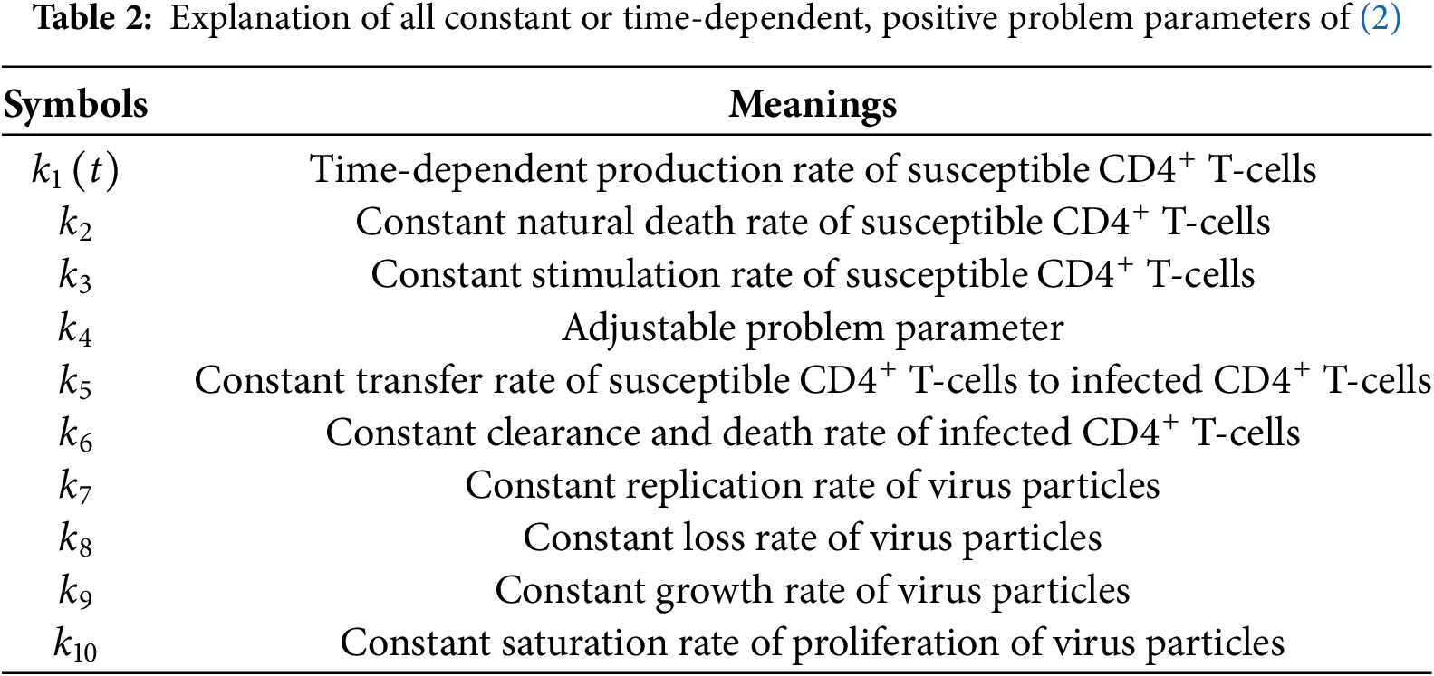
Before we continue our chronological summary of different contributions to the field of mathematical modeling of primary HIV infection, we want to introduce our model under consideration which is excellently described by Kirschner [29]. Again, we denote the density of susceptible, uninfected
where
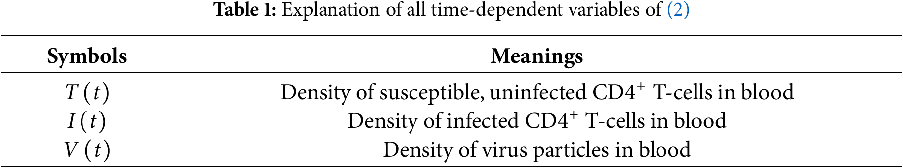
In the first equation of (2),
Now, we can complete our brief overview on mathematical modeling of primary HIV infections. In 1996, Perelson and co-authors suggested an adjustment of (1) by an infectious pool and a non-infectious pool of virions after introducing a pharmacological therapy [30]. One year later, Perelson and co-workers proposed a changed dynamical model of HIV infection under combination therapy [31]. In 1999, Perelson and Nelson reviewed some fundamental mathematical models, especially regarding the stability of systems of ordinary differential equations concerning primary HIV-infections [32]. In 2000, Stafford and co-authors specifically investigated parameter estimation of model (1) concerning data from different patients [24]. Two years later, Perelson reviewed some basic models regarding primary HIV infection with and without medical treatment [25].
A delay-based system of integro-differential equations of cell-to-cell spread of primary HIV infections was introduced by Culshaw et al. in 2003 [33]. Based on (1), Stilianakis and Schenzle recommended a time-dependent infection rate [34]. In 2009, Kamp examined different strains under HIV coreceptor switch from a dynamical perspective, where investigation of stability was mainly focused [35]. One year later, Elaiw proposed an alternation of (1) by latently infected and actively infected
We also like to briefly highlight stochastic approaches for the solution of within-host HIV models, such as those presented by Mbogo [51] and co-authors in 2013 or by Umar and co-workers [52] in 2022.
1.2 Motivation on Numerical Discretizations
While many works on mathematical models of HIV infections exist, numerical solution of these models, such as time-discrete variants of time-continuous models, is an important research topic as well. We want to summarize some studies with regard to this matter.
Many classical time integration methods such as Runge-Kutta schemes can be applied to such systems of ordinary differential equations [53,54]. As an alternative approach, Mickens popularized the concept of non-standard finite-difference methods for solving differential equations [55,56]. Let
be a system of ordinary differential equations. Often, we want to find preferably a finite-difference-scheme of the form
where
1.
2.
In 2013, Obaid et al. established a non-standard finite-difference method of development of HIV infections between hosts in a population [57]. In 2016, Yang and co-authors presented one non-standard finite-difference method for a diffusive within-host dynamics model with both virus-to-cell and cell-to-cell transmissions [58]. These authors mainly focused on analyzing stability properties for their suggested discretization method. Elaiw and Alshaikh examined the global stability of different time-discrete HIV dynamical models with three categories of infected
All in all, many studies focused mainly on stability properties of (2) and only a few non-standard finite-difference methods exist in the literature. Henceforth, our contributions can be stated as follows:
1. First, we extend some analytical results of (2) by proofs of non-negativity, boundedness of
2. As our main contribution, we suggest a novel non-standard finite-difference-method
with non-equidistant time-step sizes
3. Finally, we illustrate our theoretical findings by numerical examples.
Our work is organized as follows. After stating our main goals in Section 1, we provide analytical results of the time-continuous model (2) in Section 2. In Section 3, we examine our proposed non-standard finite-difference-method (3) thoroughly and show evidence of our theoretical results by numerical experiments in Section 4. Conclusively, we summarize our findings and possible future research directions in Section 5.
2 Analysis of the Time-Continuous Problem Formulation
Since the vectorial right-hand-side function of (2) is at least continuous, we can conclude that all solution components are at least continuously differentiable.
Before providing our analytical results, we want to summarize some important results that we need for our investigation. Let us consider the general initial-value problem
where all state variables are included in
where
holds for all
Theorem 1. If
holds for all
for all
2.2 Non-Negativity, Boundedness of
First, we want to show that possible solutions of (2) remain non-negative for all
Theorem 2. Solutions of (2) stay non-negative for all
Proof. Since all solution components of (2) are continuous, there exists a time point
holds. Let us assume that
is valid for all
Additionally, we notice that
holds for all
for all
holds for all
for all
Next, we want to prove the boundedness of
Lemma 1. The solution components
Proof. We separate this proof into two parts.
1. It has already been proven that the inequality
for all
which proves our first assertion.
2. It has also been shown that the inequality
holds because of the non-negativity of all solution components. Again, applying the comparison principle, we obtain
for all
This finishes our proof. □
As our last result of this subsection, we prove that
Lemma 2. The solution component
Proof. The differential equation for
due to the non-negativity of all solution components. Consequently, it holds
by the comparison principle for all
2.3 Existence Globally in Time
Let us define
as the right-hand-side function of (2). We notice that this function is locally Lipschitz-continuous on
Theorem 3. Solutions of (2) exist for all
Proof. We need to estimate all components of
1. We see that
holds.
2. Additionally, we notice that
is valid.
3. Furthermore, we obtain
4. Conclusively, these three inequalities yield
Finally, this proves the existence of solutions of (2) globally in time since all assumptions of Theorem 1 are fulfilled. □
By applying [[65], Corollary 2, Subchapter 2.4] and [[65], Theorem 4, Subchapter 2.4], we obtain a uniqueness result globally in time on
Theorem 4. Solutions of (2) exist uniquely for all
Proof. Let us construct the open set
holds for all
For searching equilibrium states of system (2), we need to solve the system of non-linear equations
where
2.5.1 Virus-Free Equilibrium State
It can be seen from (7) that the virus-free equilibrium state reads
Let us define the basic reproduction number
which is going to be motivated in the proof of our next statement.
Theorem 5. If
Proof. We divide our proof into different parts.
1. We first calculate the Jacobian matrix, denoted by
with entries
holds.
2. If we plug our virus-free equilibrium state (8), we obtain
Calculating the characteristic polynomial
is valid. Both eigenvalues
This finishes our argument. □
2.5.2 Virus-Endemic Equilibrium State
Here, we assume that
holds. From (7), we obtain
Since
Plugging all results of (11) into our previous equation, we get
and we can re-establish zeros of (12) by finding zeros of
Let us define the coefficients
Hence, finding zeros of (13) is equivalent to solving
Normalizing this cubic polynomial yields
This equation can be solved analytically by applying Tschirnhaus-transformation and setting
Conclusively, all solutions of (16) read
Since there is a complex interplay between initial values, problem parameters and stability of our possibly three computed equilibrium states, we want to provide a numerical algorithm for solving this problem. Our procedure is given in Algorithm 1.

We want to conclude our analytical results here with this remark.
Remark 1. As already mentioned above, we have a complex situation in case of
We would like to point out that all qualitative properties of our time-continuous model are important features that should transfer to the time-discrete setting. For that reason, we note that it is always important to examine properties of the time-continuous case rigorously. Consequently, it becomes easier to build time-discrete approximations which fulfill all these requirements.
3 Analysis of the Time-Discrete Problem Formulation Based on a Non-Standard Finite-Difference- Method
Here, we want to consider a non-equidistant partition
of our simulation time interval
for all
at a time point
at a time point
3.1 Time-Discrete Problem Formulation and Unique Solvability
Discretizing (2) by (3), we propose our non-standard finite-difference-method based solely on non-local approximations by
for all time indices
holds from the first equation of (19). The second equation of (19) implies
From the last equation of (19), we obtain
Now, we summarize our solution algorithm for (19) in Algorithm 2.
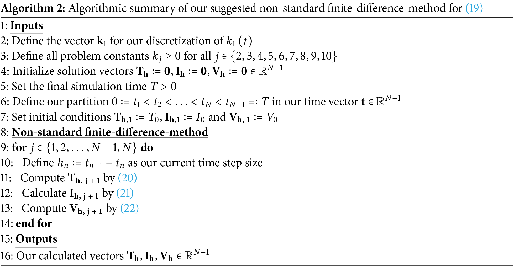
Here, we can show the unique solvability of our Algorithm 2.
Theorem 6. Our numerical solution approach in Algorithm 2 is uniquely solvable.
Proof. Since our initial conditions
3.2 Non-Negativity, Boundedness of
Let us first show that all solution components of Algorithm 2 stay non-negative.
Theorem 7. All components of our solution vectors
Proof. Our initial conditions
Now, we want to prove that every component of
Theorem 8. It holds
Proof. We separate this proof into two steps. Keep in mind that
Step 1: Let us first consider
for all
and this implies
Step 2: We want to prove our claim by induction. It obviously holds
Conclusively, our upper bound
Next, we want to show that every component of
Theorem 9. It holds
Proof. We separate this proof into two steps. Keep in mind that
Step 1: It holds
for all time-discrete indices
for all
Step 2: We want to prove our claim by induction. It obviously holds
Conclusively, our upper bound
Finally, we show that every component of
Theorem 10. It holds
Proof. We observe that
holds for an arbitrary
for an arbitrary time-discrete index
Now, we want to show our claim by induction. For
Let us now assume that
holds for an arbitrary
which finishes our claim’s proof. □
For simplicity of presentation, let us assume that
holds. Furthermore, we notice that
is valid by using (25). By applying (25) and (26), we obtain
Hence, comparing (7) and (25)–(27), we conclude that our proposed non-standard finite-difference-method possesses the same equilibrium states as the time-continuous model (2).
3.4 Convergence towards the Time-Continuous Problem Solution
To finish our theoretical observations of Algorithm 2, we show that it converges linearly towards the time-continuous solution of model (2). To begin with, we summarize all our assumptions for linear convergence of our time-discrete solution components of Algorithm 2 towards the time-continuous solution components of model (2).
(A1) We consider the time interval
(A2) Initial conditions of the time-continuous and the time-discrete problems coincide;
(A3) The time-continuous rate function
(A4) Time-continuous solution components
(A5) Set
Theorem 11. Let all aforementioned assumptions (A1)–(A5) be fulfilled. Then the time-discrete solution components converge linearly towards the time-continuous solution components if
Proof. We briefly outline our proof plan because it is relatively technical. First, let us assume that all time-continuous solution components coincide with all time-discrete solution components at a certain time point
1. For local error propagation, we assume that
hold for an arbitrary
1.1. We see that
is valid. Additionally, we observe that
holds. Application of the mean value theorem yields
Another application of the mean value theorem implies
After defining our constant
we obtain
1.2. We see that
is valid. This implies
By similar argument as before, we obtain
and
By defining the constant
we conclude
1.3. It holds
Furthermore, we obtain
By similar arguments as before, we get the estimates
and
Defining the constant
we obtain
2. In general, the points
by boundedness of all time-continuous solution components on our simulation interval
by boundedness of all time-discrete solution components for all
for all
and
for all
2.1. We see that
is valid and
and
By defining the constant
we obtain the estimate
2.2. With similar, but lengthier arguments as before, there exist non-negative constants
and
hold. Conclusively, this implies
3. Let us define
It holds
by the results of our first two steps and this can be iterated inductively. Finally, we see that
is valid because
This finishes our proof of convergence. □
We want to conclude our investigation on our proposed non-standard finite-difference method (19) with one final remark.
Remark 2. Here, we managed to show that our proposed non-standard finite-difference-method (19) is unconditionally non-negativity-preserving. Additionally, we were able to demonstrate that this time-discrete version of (2) also preserves upper bounds for
However, we would also like to discuss some potential limitations of our time-discrete analysis. In contrast to [62], we were not able to prove the global asymptotic stability of our equilibrium states. While their dynamical system consists of a polynomial right-hand-side vectorial function, we have rational functions. Additionally, we showed that even our time-continuous model possesses at most linear growth of
Here, we want to illustrate our theoretical findings by different numerical examples. In our examples, we choose an equidistant mesh, i.e., that our chosen time step size
First, we want to show that our non-standard finite-difference-method (NSFDM), in contrast to other traditional explicit time discretizations such as the explicit Eulerian method (EE) or a second-order Runge-Kutta scheme (RK2), preserves non-negativity independent of our chosen time step sizes
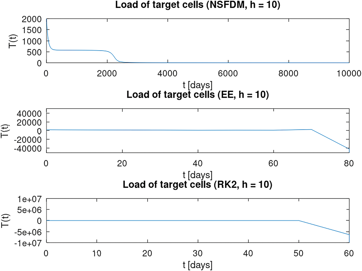
Figure 1: Numerical results of a load of target cells for
We observe that only our proposed non-standard finite-difference method from Algorithm 2 can capture non-negativity over a long time interval for a larger equidistant time step size

Figure 2: Numerical results of a load of target cells for
In this example, we want to distinguish three different situations of equilibrium states.
4.2.1 Situation 1: Virus-Free Equilibrium State
Let us take all problem parameters from Section 4.1. The exceptions are
for our example. Our numerical results can be seen in Fig. 3. Here, solid lines represent our solution components of a load of target cells, a load of infected target cells, and a load of virus cells. Dashed lines give our coordinates of the virus-free equilibrium state which are computed by

Figure 3: Numerical results of our setting in Section 4.2.1 where solid lines represent the solution components while dashed lines stand for the coordinates of the virus-free equilibrium state
We observe that our suggested non-standard finite-difference method converges to the computed coordinates of the virus-free equilibrium state.
4.2.2 Situation 2: Virus-Endemic Equilibrium State
Let us take all problem parameters from Section 4.2.1. The exception is
in this example. Our numerical results can be seen in Fig. 4. Here, solid lines represent our solution components of a load of target cells, a load of infected target cells, and load of virus cells. Dashed lines give our coordinates of the virus-free equilibrium state which are computed by

Figure 4: Numerical results of our setting in Section 4.2.2 where solid lines represent the solution components while dashed lines stand for the coordinates of the virus-endemic equilibrium state
We observe that our suggested non-standard finite-difference method converges to the computed coordinates of the virus-endemic equilibrium state.
4.2.3 Situation 3: Linear Growth of
Let us take all problem parameters from Section 4.2.1. The exception is

Figure 5: Numerical results of our setting in Section 4.2.3 where solid lines represent the solution components
4.2.4 Situation 4: Real-World Application with Some Estimated Parameters from Clinical Trials and Some Calibrated Parameters from Numerical Simulations
In this numerical experiment, we take some estimated parameter values from Kirschner’s work [29] and from [27] which have been evaluated from different clinical trials. Here, we want to show that, in particular, the load of susceptible
In Fig. 6, we see numerical approximations of our presented setting. As mentioned in [44], Kirschner’s model can capture important features of the acute and the latent phase. We observe a steep decrease of susceptible
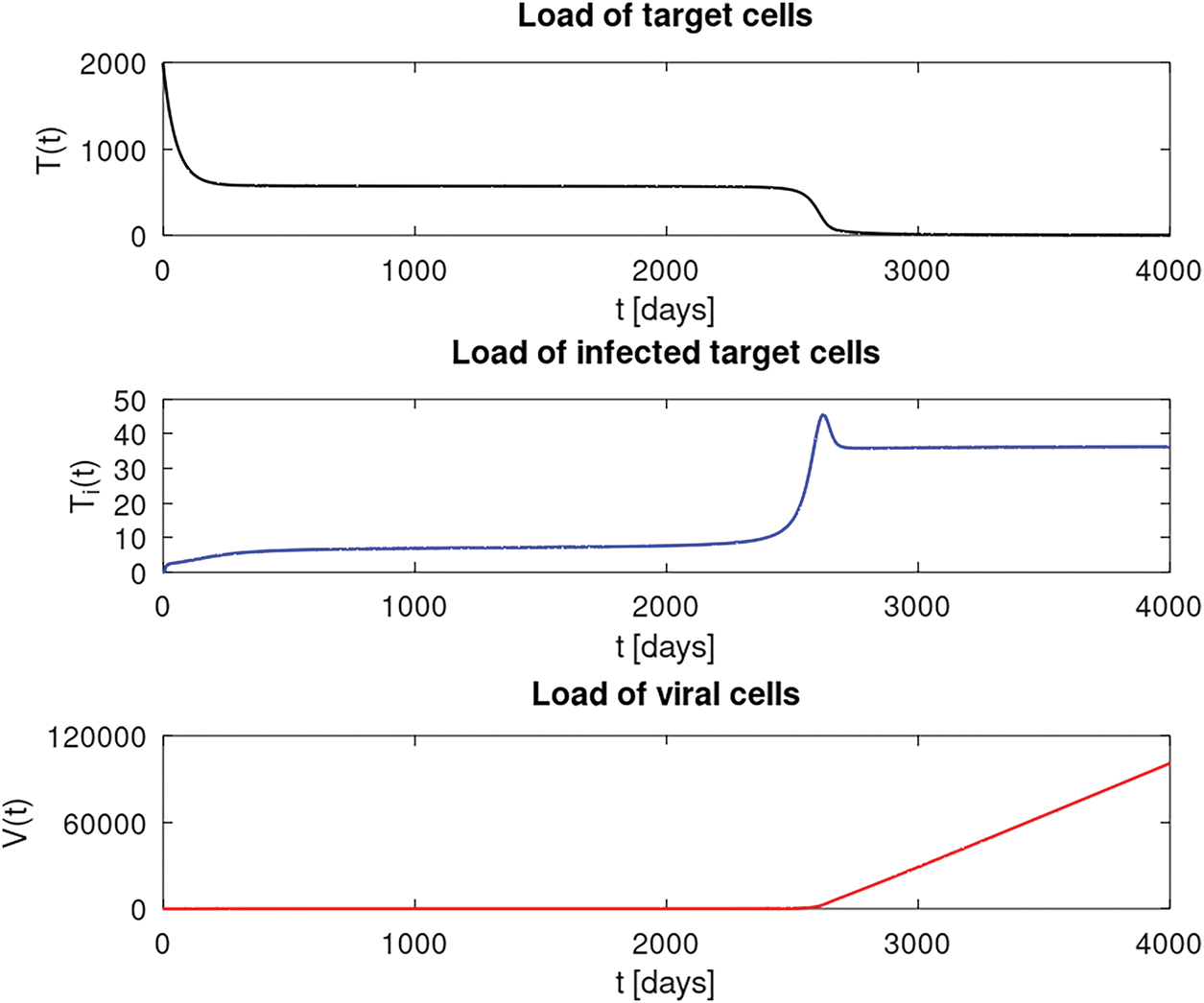
Figure 6: Numerical results of our setting in Section 4.2.4 where solid lines represent the solution components
What can be seen as a drawback of Kirschner’s model, as we have already noticed from our theoretical results in Section 2, is the linear growth of virus cells which can be explained by the last term
Conclusively, we take all problem parameters from Section 4.2.2. Here, we want to demonstrate that our proposed non-standard finite-difference-method really is a first-order method. For that purpose, we use a fine-scale solution of a fourth-order Runge-Kutta method where all solution components read
The calculated errors of our non-standard finite-difference method for different equidistant time step sizes are summarized in Table 3.
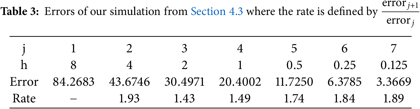
For small time step sizes, we notice that
Here, we want to summarize some of our theoretical results and of our numerical observations concerning our suggested non-standard finite-difference-method (19).
As we have already proven, our numerical solution algorithm is unconditionally stable and, in particular, it preserves non-negativity for all positive time-step sizes which is one preferable property of the time-continuous model. Hence, this is one main difference from classical Runge-Kutta time-stepping methods which are only conditionally stable and which conserve non-negativity only for a certain range of positive time-step sizes.
In terms of computational cost, since our proposed numerical solution algorithm is explicit and is of convergence order one, it is comparable to an explicit Eulerian time-stepping method concerning computational time. However, in contrast to the explicit Eulerian time-stepping procedure, our algorithm is unconditionally stable and unconditionally non-negativity-preserving. These are features that our algorithm shares with the implicit Eulerian time-stepping method. In contrast to implicit time-discretizations, our numerical solution procedure is explicit and henceforth, it avoids solutions of non-linear systems of equations in each time step.
Conclusively, our proposed non-standard finite-difference method has some interesting numerical properties which transfer from the time-continuous model to our time-discrete setting.
In this work, we re-examined a classical dynamical system for untreated HIV infections proposed by Kirschner. In particular, we proved the non-negativity of all solution components, boundedness of two solution components, at most linear growth of one solution component, existence and uniqueness of solutions, and investigated equilibrium states and local stability for the virus-free equilibrium state. With regard to the time-discrete setting, we suggested a new non-standard finite-difference-method, solely based on non-local approximations. We demonstrated that many properties of the time-continuous case transferred to the time-discrete setting. In particular, we showed that our non-standard finite-difference method is of first order. Conclusively, we strengthened our theoretical findings with different numerical examples.
Let us discuss one important limitation of Kirschner’s time-continuous model [29]. Since our proof showed that the viral load
Finishing our article, we want to sketch some potential future research directions. At first, it could be of interest to construct higher-order non-standard finite-difference-methods, compare, for example, [66]. In that work, the authors applied Richardson’s extrapolation to construct higher-order non-standard finite-difference methods for a model of malware propagation. While they achieve higher rates of convergence, preservation of non-negativity for all time-step sizes was only observed numerically. Henceforth, we stayed with a first-order approach which easily guarantees non-negativity without any restrictions on possible time-step sizes. Furthermore, in contrast to many other works, we applied a non-equidistant time grid.
From a modeling perspective, it seems interesting to add spatial inhomogeneity to Kirschner’s model by the introduction of diffusion or reaction terms. This implies that the investigated model transfers to a partial differential equation [67]. Additionally, it might be worth noticing that it is possible to implement further compartments into Kirschner’s presented model. Possible extensions might be immune responses from different cells [68] or the total amount of protein levels within a human being [69]. Depending on the structure of these higher-order dynamical systems, our ideas, presented in this article, can be extended to such models as well to create non-standard finite-difference methods which preserve important properties of the time-continuous setting. The implementation of drug therapy into Kirschner’s model has already been mentioned by Kirschner herself [29].
Acknowledgement: It is not applicable.
Funding Statement: The authors received no funding for this study.
Author Contributions: Benjamin Wacker: conceptualization, formal analysis, investigation, methodology, software, validation, visualization, writing—original draft; Jan Christian Schlüter: conceptualization, writing—review & editing. All authors reviewed the results and approved the final version of the manuscript.
Availability of Data and Materials: Our GNU Octave codes can be found under the following hyperlink https://github.com/bewa87/2025-Modified-HIV-NSFDM (accessed on 07 July 2025).
Ethics Approval: It is not applicable.
Conflicts of Interest: The authors declare no conflicts of interest to report regarding the present study.
References
1. Deeks SG, Overbaugh J, Phillips A, Buchbinder S. HIV infection. Nat Rev Dis Primers. 2015;1(1):15035. doi:10.1038/nrdp.2015.35. [Google Scholar] [PubMed] [CrossRef]
2. Mody A, Sohn AH, Iwuji C, Tan RKJ, Venter F, Geng EH. HIV epidemiology, prevention, treatment, and implementation strategies for public health. Lancet. 2024;402:471–92. doi:10.1016/S0140-6736(23)01381-8. [Google Scholar] [PubMed] [CrossRef]
3. UNAids. Fact Sheet 2024-Global HIV Statistics. 2024 [Internet]. [cited 2024 Nov 5]. Available from: https://www.unaids.org/sites/default/files/media_asset/UNAIDS_FactSheet_en.pdf. [Google Scholar]
4. Moir S, Chun TW, Fauci AS. Pathogenic mechanisms of HIV disease. Annu Rev Pathol-Mech Dis. 2011;6(1):223–48. doi:10.1146/annurev-pathol-011110-130254. [Google Scholar] [PubMed] [CrossRef]
5. Mellors JW, Rinaldo CR Jr, Gupta P, White RM, Todd JA, Kingsley LA. Prognosis in HIV-1 infection predicted by the quantity of virus in plasma. Science. 1996;272(5265):1167–70. doi:10.1126/science.272.5265.1167. [Google Scholar] [PubMed] [CrossRef]
6. McCune JM. The dynamics of CD4+ T-cell depletion in HIV disease. Nature. 2001;410(6831):974–9. doi:10.1038/35073648. [Google Scholar] [PubMed] [CrossRef]
7. Deeks SG, Walker BD. Human immunodeficiency virus controllers: mechanisms of durable virus control in the absence of antiretroviral therapy. Immunity. 2007;27(3):406–16. doi:10.1016/j.immuni.2007.08.010. [Google Scholar] [PubMed] [CrossRef]
8. Alizon S, Magnus C. Modelling the course of an HIV infection: insights from ecology and evolution. Viruses. 2012;4(10):1984–2013. doi:10.3390/v4101984. [Google Scholar] [PubMed] [CrossRef]
9. Perelson AS, Ribeiro RM. Modeling the within-host dynamics of HIV infection. BMC Biol. 2013;11(1):96. doi:10.1186/1741-7007-11-96. [Google Scholar] [PubMed] [CrossRef]
10. D’Orso I, Forst CV. Mathematical models of HIV-1 dynamics, transcription, and latency. Viruses. 2023;15(10):2119. doi:10.3390/v15102119. [Google Scholar] [PubMed] [CrossRef]
11. Ashi HA, Alahmadi DM. A mathematical model of brain tumor. Math Meth Appl Sci. 2023;46(9):10137–50. doi:10.1002/mma.9107. [Google Scholar] [CrossRef]
12. Hoang MT, Ehrhardt M. A second-order nonstandard finite difference method for a general Rosenzweig-MacArthur predator-prey model. J Comput Appl Math. 2024;444(12):115752. doi:10.1016/j.cam.2024.115752. [Google Scholar] [CrossRef]
13. Wacker B. Analysis of a finite-difference method based on nonlocal approximations for a nonlinear, extended three-compartmental model of ethanol metabolism in the human body. Math Meth Appl Sci. 2025;48(9):9975–92. doi:10.1002/mma.10858. [Google Scholar] [CrossRef]
14. Levitt MD, Levitt DG. Use of a two-compartmental model to assess pharmacokinetics of human ethanol metabolism. Alcohol Clin Exp Res. 1998;22(8):1680–8. doi:10.1111/j.1530-0277.1998.tb03966.x. [Google Scholar] [CrossRef]
15. Wacker B, Schlüter JC. Qualitative analysis of two systems of nonlinear first-order ordinary differential equations for biological systems. Math Meth Appl Sci. 2022;45(8):4597–624. doi:10.1002/mma.8056. [Google Scholar] [CrossRef]
16. Hariharan S, Shangerganesh L, Debbouche A, Antonov V. Dynamic behaviors for fractional epidemiological model featuring vaccination and quarantine compartments. J Appl Math Comput. 2025;71(1):489–509. doi:10.1007/s12190-024-02249-3. [Google Scholar] [CrossRef]
17. Wacker B, Schlüter JC. An age- and sex-structured SIR model: theory and an explicit-implicit numerical solution algorithm. Math Biosci Eng. 2020;17(5):5752–801. doi:10.3934/mbe.2020309. [Google Scholar] [PubMed] [CrossRef]
18. Wacker B, Schlüter JC. A non-standard finite-difference-method for a non-autonomous epidemiological model: analysis, parameter identification and applications. Math Biosci Eng. 2023;20(7):12923–54. doi:10.3934/mbe.2023577. [Google Scholar] [PubMed] [CrossRef]
19. Feinberg M. Foundations of chemical reaction network theory. 1st ed. Cham, Switzerland: Springer-Verlag; 2019. doi:10.1007/978-3-030-03858-8. [Google Scholar] [CrossRef]
20. Formaggia L, Scotti A. Positivity and conservation properties of some integration schemes for mass action kinetics. SIAM J Numer Anal. 2011;49(3):1267–88. doi:10.1137/100789592. [Google Scholar] [CrossRef]
21. Mincheva M, Siegel D. Nonnegativity and positiveness of solutions to mass action reaction-diffusion systems. J Math Chem. 2007;42(4):1135–45. doi:10.1007/s10910-007-9292-0. [Google Scholar] [CrossRef]
22. Hoang MT, Quy Ngo TK, Tran DH. Dynamically consistent nonstandard numerical schemes for solving some computer virus and malware propagation models. Math Found Comput. 2023;6(4):704–27. doi:10.3934/mfc.2022042. [Google Scholar] [CrossRef]
23. Wacker B. Qualitative study of a dynamical system for computer virus propagation—a nonstandard finite-difference-methodological view. Math Meth Appl Sci. 2025;48(8):9272–91. doi:10.1002/mma.10798. [Google Scholar] [CrossRef]
24. Stafford MA, Corey L, Cao Y, Daar ES, Ho DD, Perelson AS. Modeling plasma virus concentration during primary HIV infection. J Theor Biol. 2000;203(3):285–301. doi:10.1006/jtbi.2000.1076. [Google Scholar] [PubMed] [CrossRef]
25. Perelson AS. Modelling viral and immune system dynamics. Nat Rev-Immunol. 2002;2(1):28–36. doi:10.1038/nri700. [Google Scholar] [PubMed] [CrossRef]
26. Nowak MA, May RM. Mathematical biology of HIV infections: antigenic variation and diversity threshold. Math Biosci. 1991;106(1):1–21. doi:10.1016/0025-5564(91)90037-j. [Google Scholar] [PubMed] [CrossRef]
27. Perelson AS, Kirschner DE, De Boer R. Dynamics of HIV infection of CD4+ T cells. Math Biosci. 1993;114(1):81–125. doi:10.1016/0025-5564(93)90043-a. [Google Scholar] [PubMed] [CrossRef]
28. Bonhoeffer S, Nowak MA. Intra-host versus inter-host selection: viral strategies of immune function impairment. Proc Natl Acad Sci U S A. 1994;91(17):8062–6. doi:10.1073/pnas.91.17.8062. [Google Scholar] [PubMed] [CrossRef]
29. Kirschner DE. Using mathematics to understand HIV immune dynamics. Not Amer Math Soc. 1996;43(2):191–202. [Google Scholar]
30. Perelson AS, Neumann AU, Markowitz M, Leonard JM, Ho DD. HIV-1 dynamics in vivo: virion clearance rate, infected cell life-span, and viral generation time. Science. 1996;271(5255):1582–6. doi:10.1126/science.271.5255.1582. [Google Scholar] [PubMed] [CrossRef]
31. Perelson AS, Essunger P, Cao Y, Vesanen M, Hurley A, Saksela K, et al. Decay characteristics of HIV-1 infected compartments during combination therapy. Nature. 1997;387(6629):188–91. doi:10.1038/387188a0. [Google Scholar] [PubMed] [CrossRef]
32. Perelson AS, Nelson PW. Mathematical analysis of HIV-1 dynamics in vivo. SIAM Rev. 1999;41(1):3–44. doi:10.1137/S0036144598335107. [Google Scholar] [CrossRef]
33. Culshaw RV, Ruan S, Webb G. A mathematical model of cell-to-cell spread of HIV-1 that includes a time delay. J Math Biol. 2003;46(5):425–44. doi:10.1007/s00285-002-0191-5. [Google Scholar] [PubMed] [CrossRef]
34. Stilianakis NI, Schenzle D. On the intra-host dynamics of HIV-1 infections. Math Biosci. 2006;199(1):1–25. doi:10.1016/j.mbs.2005.09.003. [Google Scholar] [PubMed] [CrossRef]
35. Kamp C. Understanding the HIV coreceptor switch from a dynamical perspective. BMC Ecol Evol. 2009;9(1):274. doi:10.1186/1471-2148-9-274. [Google Scholar] [PubMed] [CrossRef]
36. Elaiw AM. Global properties of a class of HIV models. Nonlinear Anal Real World Appl. 2010;11(4):2253–63. doi:10.1016/j.nonrwa.2009.07.001. [Google Scholar] [CrossRef]
37. Lythgoe KA, Fraser C. New insights into the evolutionary rate of HIV-1 at the within-host and epidemiological levels. Proc R Soc B. 2012;279(1741):3367–75. doi:10.1098/rspb.2012.0595. [Google Scholar] [PubMed] [CrossRef]
38. Pourbashash H, Pilyugin SS, De Leenheer P, McCluskey C. Global analysis of within host virus models with cell-to-cell viral transmission. Discrete Contin Dyn Syst-B. 2014;19(10):3341–57. doi:10.3934/dcdsb.2014.19.3341. [Google Scholar] [CrossRef]
39. Shen M, Xiao Y, Rong L. Global stability of an infection-age structured HIV-1 model linking within-host and between-host dynamics. Math Biosci. 2015;263:37–50. doi:10.1016/j.mbs.2015.02.003. [Google Scholar] [PubMed] [CrossRef]
40. Wang S, Hottz P, Schechter M, Rong L. Modeling the slow CD4+ cell decline in HIV-infected individuals. PLoS Comput Biol. 2015;11(12):e1004665. doi:10.1371/journal.pcbi.1004665. [Google Scholar] [PubMed] [CrossRef]
41. Pankavich S, Parkinson C. Mathematical analysis of an in-host model of viral dynamics with spatial heterogeneity. Discrete Contin Dyn Syst-B. 2016;21(4):1237–57. doi:10.3934/dcdsb.2016.21.1237. [Google Scholar] [CrossRef]
42. Wang Y, Liu K, Lou Y. An age-structured within-host HIV model with T-cell competition. Nonlinear Anal Real World Appl. 2017;38(1):1–20. doi:10.1016/j.nonrwa.2017.04.002. [Google Scholar] [CrossRef]
43. Almocera AES, Nguyen VK, Hernandez-Vargas EA. Multiscale model within-host and between-host for viral infectious diseases. J Math Biol. 2018;77(4):1035–57. doi:10.1007/s00285-018-1241-y. [Google Scholar] [PubMed] [CrossRef]
44. Clarke C, Pankavich S. Three-stage modeling of HIV infection and implications for antiretroviral therapy. J Math Biol. 2024;88(3):34. doi:10.1007/s00285-024-02056-1. [Google Scholar] [PubMed] [CrossRef]
45. Wacker B. Revisiting the classical target cell limited dynamical within-host HIV model—basic mathematical properties and stability analysis. Math Biosci Eng. 2024;21(12):7805–29. doi:10.3934/mbe.2024343. [Google Scholar] [PubMed] [CrossRef]
46. Li S, Bukhsh I, Khan IU, Asjad MI, Eldin SM, El-Rahman MA, et al. The impact of standard and nonstandard finite difference schemes on HIV nonlinear dynamical model. Chaos Solit Fract. 2023;173(6):113755. doi:10.1016/j.chaos.2023.113755. [Google Scholar] [CrossRef]
47. Meetei MZ, DarAssi MH, Altaf Khan M, Koam ANA, Alzahrani E, Ahmadini AAH. Analysis and simulation study of the HIV/AIDS model using the real cases. PLoS One. 2024;19(6):e0304735. doi:10.1371/journal.pone.0304735. [Google Scholar] [PubMed] [CrossRef]
48. Ayele TK, Doungmo Goufo EF, Mugisha S, Asamoah JKK. Co-infection mathematical model for HIV/AIDS and tuberculosis with optimal control in Ethiopia. PLoS One. 2024;19(12):e0312539. doi:10.1371/journal.pone.0312539. [Google Scholar] [PubMed] [CrossRef]
49. Hao W, Zhang J, Peng Z, Jin Z. Evaluating the current status and strategies of achieving the 95-95-95 target for HIV/AIDS: a mathematical model. Discrete Contin Dyn Syst-B. 2025;30(10):3829–57. doi:10.3934/dcdsb.2025053. [Google Scholar] [CrossRef]
50. Teklu SW, Guya TT, Kotola BS, Lachamo TS. Analyses of an age structure HIV/AIDS compartmental model with optimal control theory. Sci Rep. 2025;15(1):5491. doi:10.1038/s41598-024-82467-8. [Google Scholar] [PubMed] [CrossRef]
51. Mbogo WR, Luboobi LS, Odhiambo JW. Stochastic model for in-host HIV dynamics with therapeutic intervention. Int Sch Res Notices. 2013;2013(1):103708. doi:10.1155/2013/103708. [Google Scholar] [CrossRef]
52. Umar M, Amin F, Al-Mdallah Q, Ali MR. A stochastic computation procedure to solve the dynamics of prevention in HIV system. Biomed Signal Process Control. 2022;78(6):103888. doi:10.1016/j.bspc.2022.103888. [Google Scholar] [CrossRef]
53. Hairer E, Wanner G, Nørsett. SP. Solving ordinary differential equations I-nonstiff problems. 2nd ed. Berlin: Springer-Verlag; 1993. doi:10.1007/978-3-540-78862-1. [Google Scholar] [CrossRef]
54. Hairer E, Wanner G. Solving ordinary differential equations II-stiff and differential-algebraic problems. 2nd ed. Berlin, Germany: Springer-Verlag; 1996. doi:10.1007/978-3-642-05221-7. [Google Scholar] [CrossRef]
55. Mickens RE. Nonstandard finite difference models of differential equations. 1st ed. Singapore: World Scientific; 1994. doi:10.1142/2081. [Google Scholar] [CrossRef]
56. Mickens RE. Advances in the applications of nonstandard finite difference schemes. Singapore: World Scientific; 2005. doi:10.1142/5884. [Google Scholar] [CrossRef]
57. Obaid HA, Ouifki R, Patidar KC. An unconditionally stable nonstandard finite difference method applied to a mathematical model of HIV infection. Int J Appl Math Comput Sci. 2013;23(2):357–72. doi:10.2478/amcs-2013-0027. [Google Scholar] [CrossRef]
58. Yang Y, Zhou J, Ma X, Zhang T. Nonstandard finite difference scheme for a diffusive within-host virus dynamics model with both virus-to-cell and cell-to-cell transmissions. Comput Math Appl. 2016;72(4):1013–20. doi:10.1016/j.camwa.2016.06.015. [Google Scholar] [CrossRef]
59. Elaiw AM, Alshaikh MA. Stability of discrete-time HIV dynamics models with three categories of infected CD4+ T-cells. Adv Differ Equ. 2019;2019(1):407. doi:10.1186/s13662-019-2338-3. [Google Scholar] [CrossRef]
60. Salman SM. A nonstandard finite difference scheme and optimal control for an HIV model with Beddington-DeAngelis incidence and cure rate. The Eur Phys J Plus. 2020;135(10):808. doi:10.1140/epjp/s13360-020-00839-1. [Google Scholar] [CrossRef]
61. Attaullah, Sohaib M. Mathematical modeling and numerical simulation of HIV infection model. Results Appl Math. 2020;7(41):100118. doi:10.1016/j.rinam.2020.100118. [Google Scholar] [CrossRef]
62. Elaiw AM, Aljahdali AK, Hobiny AD. Discretization and analysis of HIV-1 and HTLV-I coinfection model with latent reservoirs. Computation. 2023;11(3):54. doi:10.3390/computation11030054. [Google Scholar] [CrossRef]
63. Namjoo M, Razaghian S, Karami M, Aminian M. Nonstandard finite difference schemes for the HIV infection model of CD4+ T-cells. J Differ Equ Appl. 2025;31(6):864–91. doi:10.1080/10236198.2025.2470179. [Google Scholar] [CrossRef]
64. Schaeffer DG, Cain JW. Ordinary differential equations: basics and beyond. New York, NY, USA: Springer-Verlag; 2016. doi:10.1007/978-1-4939-6389-8. [Google Scholar] [CrossRef]
65. Perko L. Differential equations and dynamical systems. New York, NY, USA: Springer-Verlag; 1991. [Google Scholar]
66. Martín-Vaquero J, Martín del Rey A, Encinas AH, Hernández Guillén JD, Queiruga-Dios A, Rodríguez Sánchez G. Higher-order nonstandard finite difference schemes for a MSEIR model for a malware propagation. J Comput Appl Math. 2017;317(772):146–56. doi:10.1016/j.cam.2016.11.044. [Google Scholar] [CrossRef]
67. Ren X, Tian Y, Liu L, Liu X. A reaction-diffusion within-host HIV model with cell-to-cell transmission. J Math Biol. 2018;76(7):1831–72. doi:10.1007/s00285-017-1202-x. [Google Scholar] [PubMed] [CrossRef]
68. Liyanage YR, Kohan LM, Martcheva M, Tuncer N. Identifiability and parameter estimation of within-host model of HIV with immune response. Mathematics. 2024;12(18):2837. doi:10.3390/math12182837. [Google Scholar] [CrossRef]
69. Timsina AN, Liyanage YR, Martcheva M, Tuncer N. A novel within-host model of HIV and nutrition. Math Biosci Eng. 2024;21(4):5577–603. doi:10.3934/mbe.2024246. [Google Scholar] [PubMed] [CrossRef]
Cite This Article
 Copyright © 2025 The Author(s). Published by Tech Science Press.
This work is licensed under a Creative Commons Attribution 4.0 International License , which permits unrestricted use, distribution, and reproduction in any medium, provided the original work is properly cited.
 Downloads
 Citation Tools