Optimizing Haze Removal: A Variable Scattering Approach to Transmission Mapping

1  Introduction

Image restoration has been a significant problem in the fields of vehicle conjunction monitoring on the road [1], airborne photography [2], army applications [3], and related purposes [4]. Imaging in adverse conditions has a major impact on the restoration process and has become a challenge for various applications [5]. Unfavorable atmospheric conditions create an environment where varying density particles, such as haze and smog, are present [6]. The ambient light is typically scattered differently by these dissolved particles, which causes images taken by the camera to be distorted at that moment [7]. Low brightness and poor contrast are issues with these photos, which have a big impact on various activities of image processing applications like segmenting images [8], identifying targets [9], tracing objects of desire, etc. [10,11]. Furthermore, since these foreign particles generate a varying scattering environment inside a single image, degraded photos have different haze densities [12]. Therefore, recovering a perfect image from a murky one is a challenging task. Defogging the distorted images for use in computer vision applications requires an effective haze removal algorithm that considers the variation of scattering.

The atmospheric scattering model described in the literature serves as the foundation for existing single-image dehazing methods. This method produces better restoration results by estimating depth, transmission, and ambient light. The formation of an unclear image is explained by the atmospheric scattering model in the following way:

If(x)=Rd(x)tr(x)+A(1−tr(x))(1)

where If(x) is the intensity of input at position x, Rd(x) is the glow of the reinstated image, tr(x) is the transmission map, and A is atmospheric light. Additionally, transmissivity is determined as:

tr(x)=e−βd(x)(2)

where β and d(x) are the scattering coefficient and scene depth, respectively. Therefore, two parameters, β and d(x), are the only ones used in the calculation of the transmission map [5,9]. Over the previous two decades, numerous researchers [13–17], have presented their works on the calculation of depth d(x). It explains how the haze changes linearly in the image itself. The bottom and top sides of a 2-D projection of a 3-D scene determine the image’s objects, both close and far away, respectively [18–21]. Similarly, the top side of any hazy image will always have more fog than the bottom since fog density is always higher for distant things. For precise transmission map calculations, a rectilinear depth model may be helpful because the amount of fog grows linearly with depth [22]. In the previous decade, numerous scholars created a linear model by bearing these factors in mind, as is explained in the succeeding paragraph. Nayar et al. [13] have given a method in which, by comparing two images taken under various atmospheric situations, it was possible to determine the scene depth. Additionally, to acquire the scene depth required by the transmission function, Oakley et al. [23] explained the technique for minimizing this degradation in conditions where the scene geometry is known. Afterward, Narasimhan et al. [24] offered a technique to locate the sky zone manually in an image to determine the scene depth. The aforementioned techniques, meanwhile, are frequently ineffective in actual practice. For dehazing an image, He et al. [25] developed the dark channel prior method. Due to its simplicity and efficacy compared to the prior methods, this method attracted a lot of attention. Further, in order to recover the densely hazy images, Zhu et al. [15] have given a technique that is based on color attenuation, w.r.t. the difference between saturation and intensity value, the prior color attenuation characterizes the fog changes. Real-time defogging for surveillance applications is made possible by using color channel prior knowledge, which enables the rapid computation of the transmission map for a piece of pixel in the unique image. Raikwar et al. [16] introduced an enhanced linear depth system that integrates a hue factor into the depth calculation formula, which is dependent on the variation between saturation and the combination of hue and intensity. Assuming homogeneous scattering in the local area, it has been discovered that the depth maps created up to this point compute the transmissivity with constant values of the scattering coefficient. For calculating the transmission map, the scattering coefficient plays a role that is nearly as important as that of the depth map, as variations in the scattering medium lead to changes in haze thickness. Therefore, it is not appropriate to take the value of β as constant over the entire image. Selecting various values of β, such as β > 1, β = 1, and β < 1, will generally allow us to see how β affects the restored image, and that effect can be easily observed in Fig. 1. Fig. 1a shows two hazy input images of different locations, though the restored images are shown in Fig. 1b using β > 1. Through Fig. 1b, it is clear that the fog in the background has been removed, causing the foreground to appear darker or disturbed (as indicated by the red line in the figure). Contrarily, for β < 1, the fog has a minimal defogging effect in the background and is primarily removed from the foreground of photographs, as highlighted by the red line in Fig. 1d. Consequently, as can be seen in Fig. 1c, β = 1 produced uniform defogging in the backgrounds and foregrounds. As far as we know, the variable scattering concept has not yet been taken into account by any de-fogging algorithms. To significantly improve defogging techniques, it is necessary to develop a scattering model that incorporates changeable values of β. With this information in mind, this article presents a model created using the linear regression technique, which accounts for variations in β based on the fog density in the image. An improved transmission map that serves the intended restoration objective is obtained using the proposed approach. In contrast, the depth map is calculated using the color attenuation prior method from [15,16], the atmospheric light is approximated employing the technique from [25], and the computation of Rd(x) is performed using (1). The rest of the article is structured as follows: Section 2 discusses the color attenuation prior-based restoration approach. In Section 3 suggested technique is described for calculating β. The experimental evaluation is discussed in Section 4, and lastly, Section 5 provides the concluding remarks.

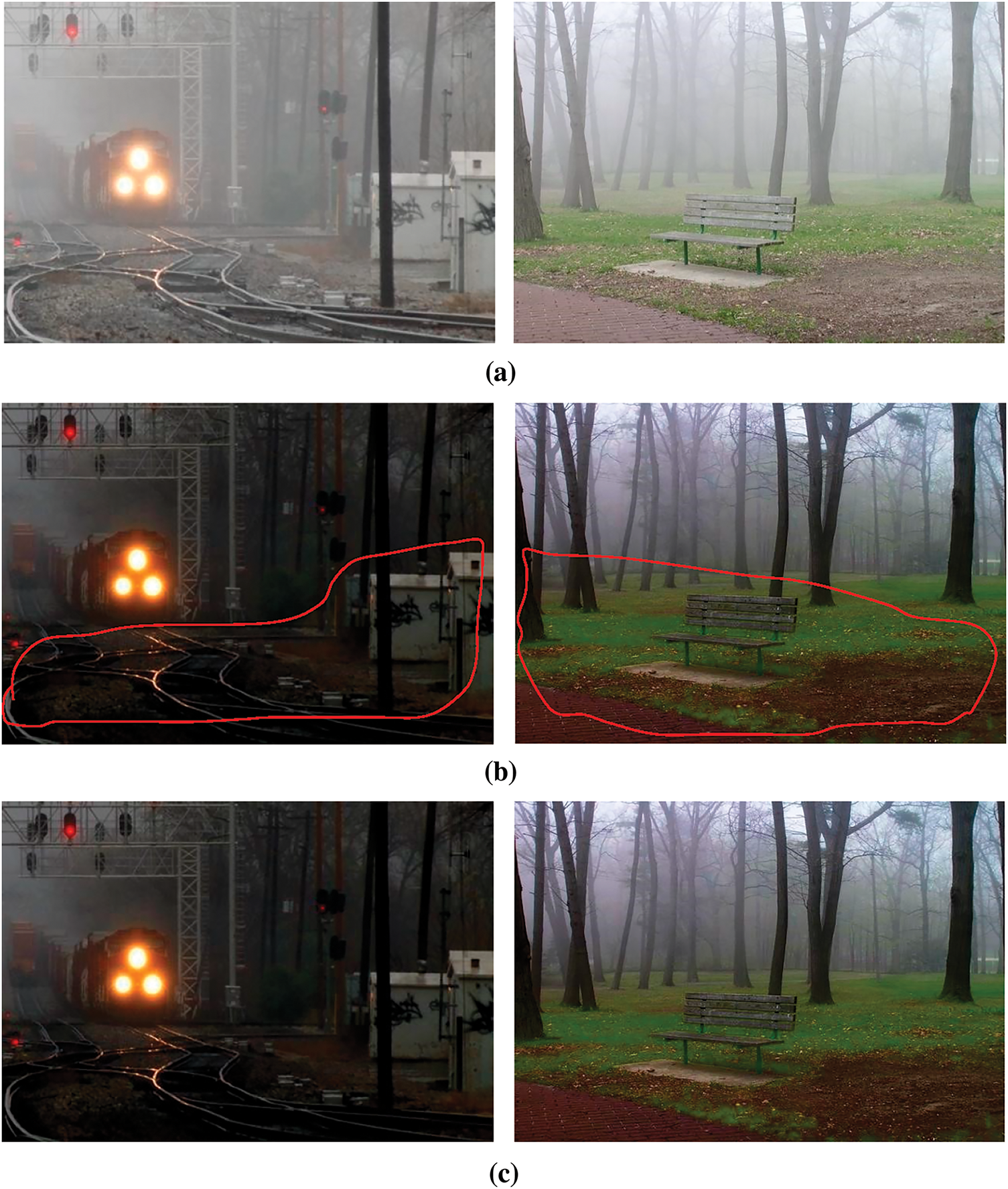
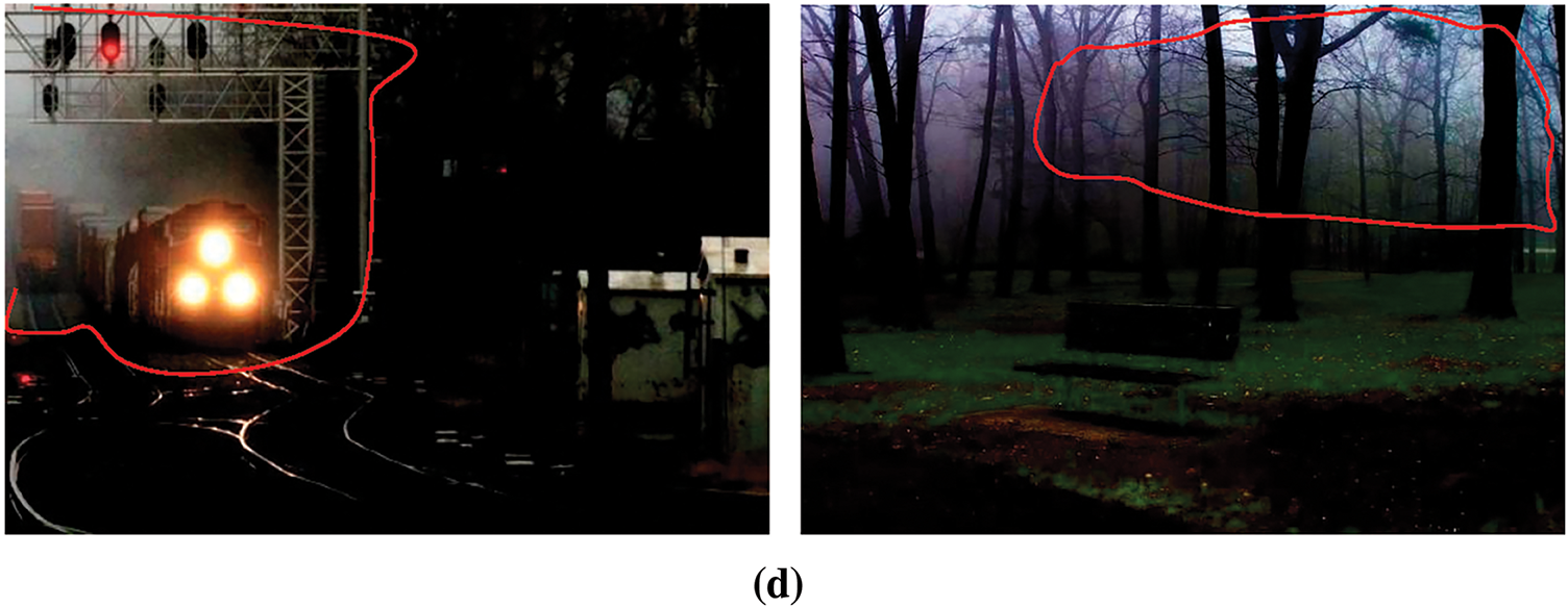
Figure 1: Analysis of impact raised due to variation of β; (a) Foggy input picture, (b–d) recovered pictures with β < 1, β = 1, and β > 1 correspondingly

2  Color Attenuation-Based Recovery Technique

The algorithm for the restoration of a foggy image is created using the atmospheric scattering model that is given in Eqs. (1) and (2). According to (1), the image restitution process involves four key factors: scene depth, transmissivity, atmospheric light, and picture radiance retrieval. In the next subsections, these four elements are briefly discussed.

2.1 Estimation of Scene Depth

Removing fog from a single image remains a significant challenge in computer vision due to the limited structural information available about the scene. A notable advancement in this area is the Color Attenuation Prior (CAP) proposed by Zhu et al. [15], which leverages the Hue, Saturation, and Value (HSV) color space for depth estimation. This method is based on the observation that haze concentration generally increases with scene depth, leading to the assumption that scene depth d(x) is positively correlated with haze concentration c(x), which, in turn, is related to the difference between pixel value and saturation: d(x) ∝ c(x) ∝ v(x) − s(x).

Building on this assumption, Zhu et al. [15] proposed a linear depth estimation model defined as: d(x)=θ0+θ1v(x)+θ2s(x) where d(x) represents scene depth, v(x) is brightness, s(x) is saturation, and (θ0,θ1,θ2) are linear coefficients learned from a training dataset comprising hundreds of diverse images across various scenes and locations.

To improve the linearity and accuracy of this model, Raikwar and Shashikala [16] extended it by incorporating the hue component. Their results showed that as scene depth or fog concentration increases, the difference between saturation and the sum of brightness and hue also increases, leading to a more robust linear depth model.

In this paper, we adopt both depth estimation approaches [15,16] to compute the scene depth, which is then used to generate the transmission map (transmissivity) essential for haze removal.

2.2 Calculation of Transmissivity

The scattering coefficient β and scene depth are needed for the calculation of the transmission map using (2). In this process, the scene depth d(x) is initially established by utilizing either [15] or [16]. The transmissivity is then refined using a median filter to keep the current edges. As a result, the raw depth map can be described as:

dr(x)=medy∈Ωr(x)[d(y)](3)

where dr(x) is a raw depth map with size r, and Ω(x) is a filter of r × r zone centring on x. Yet, certain blocking artifacts may still be present as a result of the mask-based processing, and these can be eliminated with an image-guided filter, yielding d0(x). Furthermore, the magnitude of β is crucial for scene approximation. The approaches [15,16] assume that atmospheric scattering is homogeneous throughout the scene, resulting in a constant value of β. Consequently, the redefined term for the transmissivity could be expressed as follows:

tr(x)=exp⁡(−β×d0(x))(4)

2.3 Approximation of Ambient Light & Image Brightness Restoration

The color attenuation-supported picture defogging method arranges the projected depth map in decreasing order of brightness value to determine atmospheric light A. Bright regions, which are often found in remote locations on the map, are chosen by selecting the upper 0.1% of pixels as targeted ambient bright areas. The brightness of these pixels is compared in the foggy image, and the pixel with the highest brightness is chosen as the ambient light A. This method gives a rapid and precise estimation of ambient light. After calculating the transmission map tr(x) and the atmospheric light A, the restored image Rd(x) can be obtained using the following relationship:

Rd(x)=If(x)−Amax(tr(x),0.1)+A(5)

where 0.1 serves as a cut-off point to keep the denominator from becoming small enough.

2.4 Issues

In general, the transmission map plays an important role in determining the efficacy of the fog removal algorithm. According to Eq. (2), two factors (i) scene depth (d(x)) and (ii) scattering coefficient (β) are used to calculate the transmission map. According to (2), the transmission map is calculated using two factors: (i) scene depth (d(x)) and (ii) scattering coefficient (β). According to past research, the majority of researchers only attempted to improve scene depth to calculate the transmission map, while they regarded the scattering coefficient’s value as unity under the presumption that the atmospheric disturbances are uniform throughout the whole area of the foggy image. The following conclusions are drawn from this study:

(i)   Since the atmosphere’s particles vary in size and orientation, when light from the entire atmosphere passes through them, it is scattered in all directions. As a consequence, whenever the image is taken, it exhibits non-homogeneous disruption. This theory addresses the question of how scattering coefficients, previously assumed to be uniform, can remain constant even when the disturbance is not homogeneous.

(ii)   The fog is not distributed equally across the entire picture. If the scattering coefficient were treated as a constant in this situation, it might differently affect the recovery of colors in the foreground and background, as illustrated in Fig. 1.

The observations cited above demonstrate that the transmission map’s functionality and the defogging algorithm’s effectiveness may both suffer from a constant value of scattering coefficient. The variable scattering coefficient may be able to aid with the aforementioned issues as well as improve the overall effectiveness of the defogging method. This motivates the development of a variable scattering coefficient design for fog removal methods. This article’s main contribution can be summed up as follows:

1.   When computing scene depth using methods from [15,16], the HSV color space components are adjusted to establish a relationship in which brightness and hue increase, while saturation decreases with perceived depth. Furthermore, analysis of the HSV matrices shows that the ratio of the difference to the sum of saturation and intensity values varies linearly across the image. This observation is used to develop an algorithm that dynamically adjusts the scattering coefficient for image defogging.

2.   The issue of color fidelity is addressed by incorporating a spatially variable scattering coefficient, β(x), into existing defogging techniques. However, preserving image edges remains a challenge. To mitigate edge degradation, we evaluated several filters reported in the literature and found that median filtering is most suitable, as it enhances visibility while effectively preserving edge details.

3  Suggested Approach to Estimating Atmospheric Scattering and Updated Transmissivity

As discussed in previous sections, the transmission map can be enhanced by developing it with a variable scattering coefficient β(x) for better recovery of the hazy pictures. Consequently, this section introduces a pattern-based linear model for calculating the scattering coefficients of the input foggy image. In any given hazy image, the fog density generally increases from the bottom to the top. Fog is primarily caused by foreign particles, such as moisture, dust, smog, and murk, suspended in the air. The scattering of these particles is affected by their properties, such as dimension, dispersion, or positioning, which are never entirely uniform. The varying particle sizes result in a variable-density scattering medium in the atmosphere, complicating the prediction of a variable scattering coefficient model. Moreover, several linear models have been developed in the literature [15,16,25] for determining depth, considering that fog density varies linearly with depth. In a similar way, and taking the same factors into account, the scattering map can also be produced.

In general, three separate information planes, like HSV or RGB, are used to model color images. The scattering map is created using information from any foggy image’s HSV model. Several studies have been conducted on various foggy images to explore the potential of finding a relationship between scattering and the values of HSV planes. In essence, the tests are based on random procedures carried out on the HSV values of chosen images that are blurry. Experimental analysis statistics reveal that the ratio between the difference and the sum of saturation and brightness values is directly linked to the distribution of the scattering medium.

β(x)∝v(x)−s(x)v(x)+s(x)(6)

A linear model for the variable scattering coefficient is suggested, as presented in (7), based on an approximation of (6), which indicates the concentration of scattering particles.

β(x)=c1+c2η(x)+c3χ(x)+ε(x)(7)

where η(x)=v(x)v(x)+s(x) and χ(x)=s(x)v(x)+s(x) are the normalization factors for the brightness and saturation of a hazy picture. Here, c1, c2, and c3 are the unidentified linear constants, and ε(x) represents an arbitrary error in the scattering model, characterized as an arbitrary picture with zero mean and variance σ2 (i.e., ε(x)∼N(0, σ2)).

To reduce the square of error, the optimal values of linear coefficients are computed as follows:

(ε(x))2=(β(x)−c1−c2η(x)−c3χ(x))2≅0(8)

The mathematical method of calculating linear coefficients, known as regression analysis, is predicated on the idea that the sum of the squared errors from the n samples has to be kept to a minimum. For conducting the regression examination, the linear method (7) can be rewritten in its globalized system as:

βi(x)=c1+c2ηi(x)+c3χi(x)+εi(x)(9)

Likewise, stochastic errors might be globalized as follows:

εi(x)=βi(x)−c1−c2ηi(x)−c3χi(x)(10)

Afterward, squares of errors are calculated and combined, which is given as:

E=ε12(x)+ε22(x)+ε32(x)+…+εn2(x)(11)

or

E=∑i=1n(εi(x))2=∑i=1n[βi(x)−(c1+c2ηi(x)+c3χi(x))]2(12)

Differentiate (12) partially about c1, c2, and c3, and equate it to zero to reduce the value of error E.

∂E∂c1=0=−2[β1(x)−(c1+c2η1(x)+c3χ1(x))]−2[β2(x)−(c1+c2η2(x)+c3χ2(x))]−…−2[βn(x)−(c1+c2ηn(x)+c3χn(x))](13)

∂E∂c2=0=−2η1(x)[β1(x)−(c1+c2η1(x)+c3χ1(x))]−2η2(x)[β2(x)−(c1+c2η2(x)+c3χ2(x))]−…−2ηn(x)[βn(x)−(c1+c2ηn(x)+c3χn(x))](14)

∂E∂c3=0=−2χ1(x)[β1(x)−(c1+c2η1(x)+c3χ1(x))]−2χ2(x)[β2(x)−(c1+c2η2(x)+c3χ2(x))]−…−2χn(x)[βn(x)−(c1+c2ηn(x)+c3χn(x))](15)

Eqs. (13)–(15) are simplified as:

∑i=1nβi(x)=nc1+c2∑i=1nηi(x)−c3∑i=1nχi(x)(16)

∑i=1nβi(x)×ηi(x)=c1∑i=1nηi(x)+c2∑i=1nηi2(x)−c3∑i=1nχi(x)×ηi(x)(17)

∑i=1nβi(x)×χi(x)=c1∑i=1nχi(x)+c2∑i=1nηi(x)×χi(x)−c3∑i=1nχi2(x)(18)

To determine the optimal values for scattering coefficients c1, c2, and c3, above mentioned equation could be used. However, solving these equations requires the values of the variables ∑i=1nβi(x),∑i=1nηi(x)and∑i=1nχi(x). Hence, these variables could be derived using a dataset which have hazy pictures along with ground truth pictures. This dataset can be generated using 500 clear pictures taken from the Google Images dataset. After that, hazy pictures are developed using the model given in (1), which produces the i-th hazy picture, If(x) for each recovered picture Rd(x). Once If(x) is obtained for each picture, the hue, saturation, and brightness components are extracted. Subsequently, the necessary matrices for these three variables are computed. The hazy picture developing model (1) is utilized to create the i-th hazy picture, If(x), for each lucid picture Rd(x). Afterward, obtaining If(x) for each picture, the hue, saturation, and brightness components are separated. Subsequently, the necessary matrices for the three variables are computed. The three matrices previously mentioned are used to create the sample space for fitting the curve of (12) using the least squares regression approach, as explained in (16)–(18). This allows for the determination of the values of the linear coefficients. Algorithm 1 can be utilized to compute the required values of variables c1, c2, and c3 as delineated below:

The linear coefficient values obtained using Algorithm 1 are c1 = 0.8612, c2 = 0.8059, and c3 = −0.65525. To generate a transmission map, the scattering map is modeled using both the estimated linear coefficients and (7). As a result, the redeveloped form of the transmission map could be expressed as follows:

tr(x)=exp⁡(−β(x)×d0(x))(19)

tr(x)=exp⁡(−(c1×d0(x)+c2η(x)×d0(x)+c3χ(x)×d0(x)+ε(x)×d0(x)))(20)

Additionally, the outcomes of current approaches have improved with the help of (20), and the efficiency of the suggested model is evaluated in the following section.

4  Experimental Results and Analysis

To compare the performance of the suggested technique with existing methods, both qualitative and quantitative analyses were conducted in MATLAB 19 on a 64-bit Core i7 Processor with 6 GB RAM [4,15,16,25]. The test images were selected from available datasets, including Frida2 [26] and the Waterloo IVC Dehazed Image Database [27]. The dataset included real-world foggy photos captured at various times of the day, morning, afternoon, and night.

4.1 Qualitative Analysis

The quality evaluation was conducted by simulating two existing methods [15,16] using the proposed transmission model and a specified value of β on several sets of images, as illustrated in Fig. 2. The figure consists of 7 rows and 5 columns of various images. For qualitative evaluation purposes, the arrangement of the figures is as follows: column 1 contains the original foggy images; column 2 shows the results of method [15] with a constant β; column 3 shows the results of method [15] with the proposed β(x); column 4 shows the results of method [16] with a constant β; and column 5 shows the results of method [16] with the proposed β(x).

Figure 2: Evaluation of suggested and standing methods on actual creation pictures. (a) foggy input pictures; (b) Outcomes of [15] and (d) Outcomes of [16], with persistent β; (c) Outcomes of [15] and (e) Outcomes of [16] using the suggested scattering model with variable β

Additionally, to illustrate the performance of the proposed method more clearly, row 5 presents a zoomed-in version of row 4. All of the visuals in Fig. 2 demonstrate that the proposed scattering model provides superior visibility compared to the result obtained from the existing techniques. In other words, the performance of the existing methods improves when the proposed transmission map is used in place of their original one.

4.2 Quantitative Analysis

This analysis includes several performance metrics that are described in [27,28] and are calculated to support the defogged image’s quality. This assessment offers a solid foundation for measuring how well algorithms can restore deteriorated edges and improve contrast, structure-preserving, and visibility. Further, simulations have been conducted utilizing the proposed and existing single image defogging techniques [4,15,16,25] to conduct the qualitative analysis, and Figs. 3–8 illustrate the acquired outcomes. On the images in Figs. 3–8, a quantitative evaluation has been done using the following performance measuring parameters, and the acquired outcomes are shown in Table 1.

Figure 3: Zoomed fogy picture with less background (a) Foggy input picture. (b–e) Recovered pictures [4,15,16,25], and (f) Recommended tactic

Figure 4: Visual comparison of fogy morning picture of policeman discharging duty (a) Foggy input picture. (b–e) Recovered pictures [4,15,16,25], and (f) Recommended tactic

Figure 5: Visual comparison of challenge fogy picture of railway tracks (a) Foggy input picture. (b–e) Recovered pictures [4,15,16,25], and (f) Recommended tactic

Figure 6: Fogy image of airport with deep background (a) Foggy input picture. (b–e) Recovered pictures [4,15,16,25], and (f) Recommended tactic

Figure 7: Synthetic objective testing picture (a) Foggy input picture. (b–e) Recovered pictures [4,15,16,25], and (f) Recommended tactic

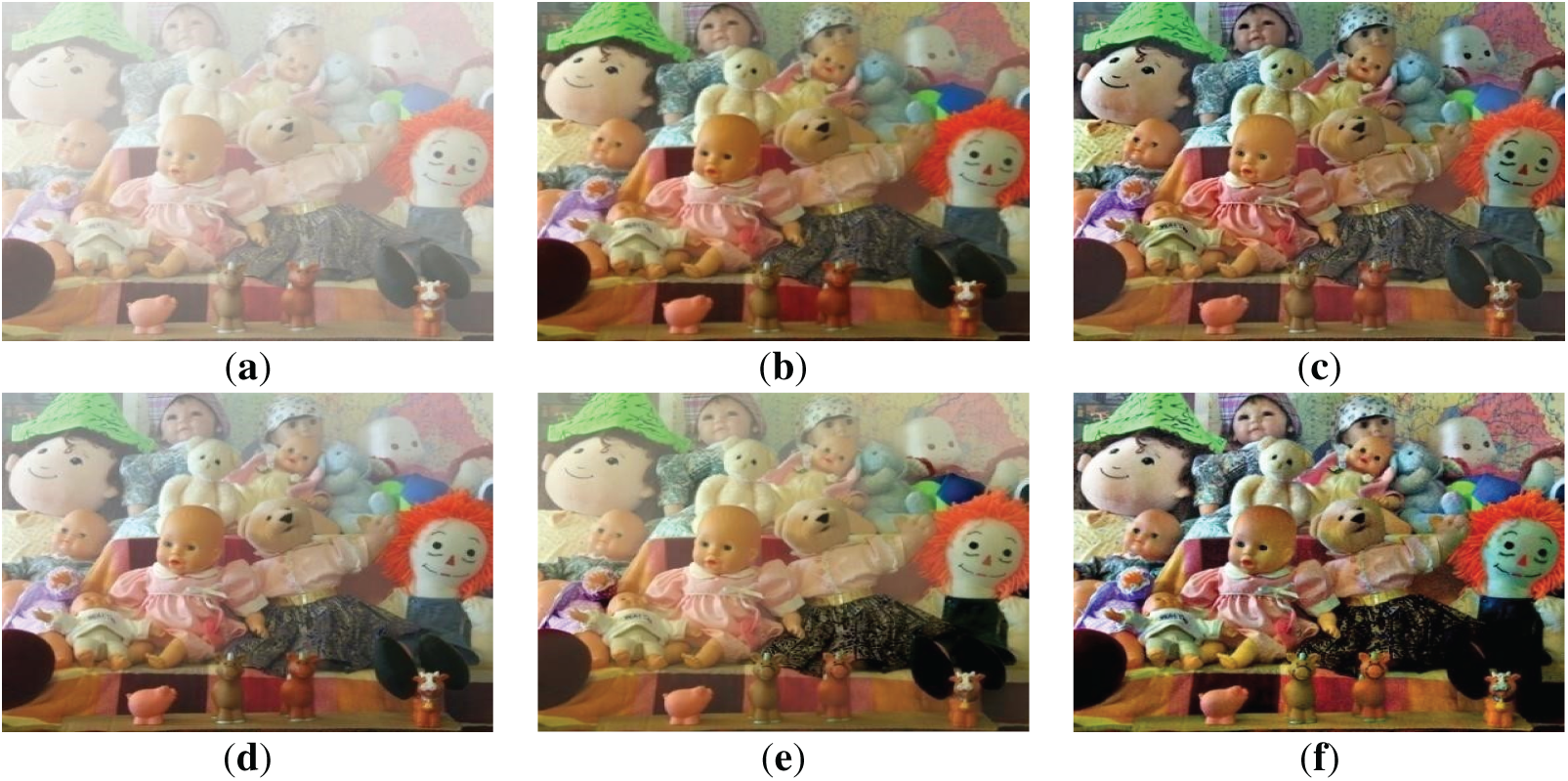
Figure 8: Synthetic testing images with multiple colors (a) Foggy input picture. (b–e) Recovered pictures [4,15,16,25], and (f) Recommended tactic

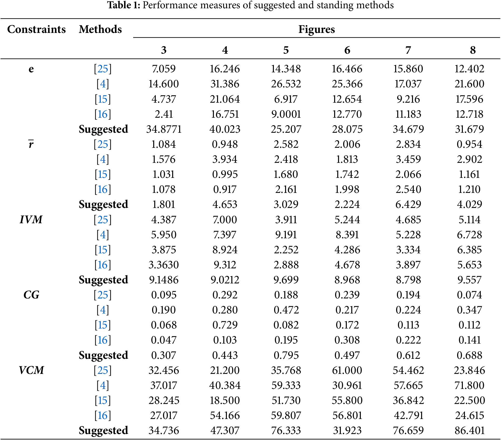
Blind Assessment: To evaluate the capacity of an algorithm used for the assessment of retaining and enhancing edges, two parameters, e, and r¯ are used.

Greater values of these parameters indicate that the suggested method can improve the level of visibility and preserve edges. Table 1 makes it abundantly clear that the suggested model has improved the values of these two descriptors.

Image Visibility Measure (IVM): The visible edge segmentation-based assessment parameter was suggested by Yu et al. [29]. According to Yu et al., an image that has been defogged will have better visibility with a larger value for this attribute. The proposed model’s ability to improve the IVM is justified by Table 1.

Contrast Gain (CG) and Visual Contrast Measure (VCM): The performance of the various defogging methods is also evaluated using these two attributes. For this, Tripathi et al. [3] and Jobson et al. [30] suggested CG and VCM to list the level of visibility in recovered images. Both of these parameters need to be larger for clear pictures than the unclear ones. Table 1 shows that utilizing the suggested model, the derived values of CG and VCM are significantly greater for each of the six test images. Furthermore, the suggested method is more efficient for non-reference-based analysis, whereas reference-based analysis also allows for quantitative analysis of the recovered image. Peak Signal to Noise Ratio (PSNR) and Structure Similarity Index Measure (SSIM) are reference-based parameters measured on test images (with the original scene) from the RESIDE [31] dataset, which is ordinarily used as a test image in numerous current dehazing approaches.

Simulations have been performed on both proposed and existing algorithms [4,15,16,25], In Table 2, we used the SOTS (Synthetic Objective Testing Set) subset of the RESIDE dataset for quantitative evaluation, as it provides clean ground truth images suitable for benchmarking dehazing algorithms. Due to computational and resource limitations, we focused on RESIDE-SOTS in this article.

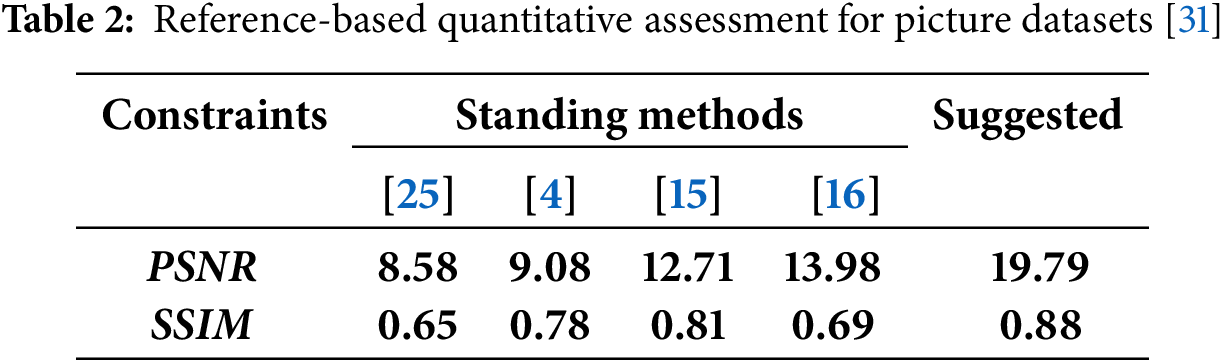
Table 2 reveals that the average values of PSNR and SSIM for the dataset [31] are appreciably good for the proposed model. Last but not least, average values for each non-reference-based parameter are calculated and presented as a bar chart as depicted in Fig. 9. It is evident from Fig. 9 that the proposed haze removal approach demonstrates superior performance in all aspects compared to other current methods [4,15,16,25].

Figure 9: Assessment of all the performance constraints for existing [4,15,16,25] and recommended tactics

5  Conclusion

Removing fog from a single image presents a significant challenge for most consumer and computer vision applications. The effectiveness of the fog removal process depends on the accuracy of estimating the transmission map, which in turn relies on precise scene depth assessment and a constant scattering coefficient, β. Furthermore, the current technique only aims to increase scene depth while maintaining a constant β. However, the haze removal method might perform more effectively with a transmission map based on variable scattering. As a result, an updated transmission map model that accounts for fluctuations in scattering information in foggy images is proposed. For effective image restoration, this updated transmission map is generated using the proposed scattering model combined with scene depth from existing approaches. Experimental findings show that the suggested model outperforms current fog removal methods in both qualitative and quantitative analyses. Moreover, the results suggest that the revised transmission map addresses established issues such as edge preservation and chromatic constancy.

A significant limitation of the proposed work is the increased computational complexity required to compute β(x), which scales with n×m compared to using a constant β. Additionally, it raises hardware complexity when implemented in hardware. However, these limitations are acceptable given the substantial improvement in image restoration quality.

Acknowledgement: The authors extend their appreciation to the Deanship of Research and Graduate Studies at King Khalid University for funding this work through Large Research Project under grant number RGP2/274/46.

Funding Statement: The Deanship of Research and Graduate Studies at King Khalid University funded this work through a Large Research Project under grant number RGP2/274/46.

Author Contributions: Gaurav Saxena has developed the methodology, Kiran Napte & Neeraj Kumar Shukla conceived the experiments, and Sushma Parihar analyzed the results. All authors reviewed the results and approved the final version of the manuscript.

Availability of Data and Materials: The datasets analyzed during the current study are available at: Dataset’A: https://ivc.uwaterloo.ca/database/dehaze.html (accessed on 01 January 2025), Dataset’B: http://perso.lcpc.fr/tarel.jean-philippe/bdd/frida.html (accessed on 01 January 2025).

Ethics Approval: Not applicable.

Conflicts of Interest: The authors declare no conflicts of interest to report regarding the present study.

References

1. Hautiere N, Tarel JP, Aubert D. Towards fog-free in-vehicle vision systems through contrast restoration. In: 2007 IEEE Conference on Computer Vision and Pattern Recognition; 2007 Jun 17–22; Minneapolis, MN, USA. p. 1–8. doi:10.1109/CVPR.2007.383259. [Google Scholar] [CrossRef]

2. Woodell G, Jobson DJ, Rahman ZU, Hines G. Advanced image processing of aerial imagery. In: Visual information processing XV. Orlando, FL, USA: SPIE; 2006. 62460E p. doi:10.1117/12.666767. [Google Scholar] [CrossRef]

3. Tripathi A, Mukhopadhyay S. Removal of fog from images: a review. IETE Tech Rev. 2012;29(2):148. doi:10.4103/0256-4602.95386. [Google Scholar] [CrossRef]

4. Raikwar SC, Tapaswi S. Adaptive dehazing control factor based fast single image dehazing. Multimed Tools Appl. 2020;79(1):891–918. doi:10.1007/s11042-019-08120-z. [Google Scholar] [CrossRef]

5. Ngo D, Lee GD, Kang B. Improved color attenuation prior for single-image haze removal. Appl Sci. 2019;9(19):4011. doi:10.3390/app9194011. [Google Scholar] [CrossRef]

6. Saxena G, Bhadauria SS, Singhal SK. Performance analysis of single image fog expulsion techniques. In: 2021 10th IEEE International Conference on Communication Systems and Network Technologies (CSNT); 2021 Jun 18–19; Bhopal, India. p. 182–7. doi:10.1109/csnt51715.2021.9509733. [Google Scholar] [CrossRef]

7. Bhamidipati RG, Jatoth RK, Naresh M, Surepally SP. Real-time classification of haze and non-haze images on Arduino Nano BLE using Edge Impulse. In: 2023 4th International Conference on Computing and Communication Systems (I3CS); 2023 Mar 16–18; Shillong, India. p. 1–7. doi:10.1109/I3CS58314.2023.10127312. [Google Scholar] [CrossRef]

8. Tang Z, Zhang X, Li X, Zhang S. Robust image hashing with ring partition and invariant vector distance. IEEE Trans Inf Forensics Secur. 2016;11(1):200–14. [Google Scholar]

9. Choi LK, You J, Bovik AC. Referenceless prediction of perceptual fog density and perceptual image defogging. IEEE Trans Image Process. 2015;24(11):3888–901. doi:10.1109/TIP.2015.2456502. [Google Scholar] [PubMed] [CrossRef]

10. Sankaraiah YR, Guru M, Reddy P, Venkata O, Reddy P, Muralikrishna K, et al. Deep learning model for haze removal from remote sensing images. Turk J Comput Math Educ. 2023;14(2):375–84. doi:10.17762/turcomat.v14i2.13662. [Google Scholar] [CrossRef]

11. Khade PI, Rajput AS. Chapter 8—efficient single image haze removal using CLAHE and Dark Channel Prior for Internet of multimedia things. In: Shukla S, Singh AK, Srivastava G, Xhafa F, editors. Internet of multimedia things (IoMT). Cambridge, MA, USA: Academic Press; 2022. p. 189–202. doi:10.1016/b978-0-32-385845-8.00013-7. [Google Scholar] [CrossRef]

12. Babu GH, Venkatram N. ABF de-hazing algorithm based on deep learning CNN for single I-Haze detection. Adv Eng Softw. 2023;175(9):103341. doi:10.1016/j.advengsoft.2022.103341. [Google Scholar] [CrossRef]

13. Nayar SK, Narasimhan SG. Vision in bad weather. IEEE Int Conf Comput Vis. 1999;2:820–7. doi:10.1109/iccv.1999.790306. [Google Scholar] [CrossRef]

14. Tan KK, Oakley JP. Physics-based approach to color image enhancement in poor visibility conditions. J Opt Soc Am A. 2001;18(10):2460–7. doi:10.1364/josaa.18.002460. [Google Scholar] [PubMed] [CrossRef]

15. Zhu Q, Mai J, Shao L. A fast single image haze removal algorithm using color attenuation prior. IEEE Trans Image Process. 2015;24(11):3522–33. doi:10.1109/TIP.2015.2446191. [Google Scholar] [PubMed] [CrossRef]

16. Raikwar SC, Tapaswi S. An improved linear depth model for single image fog removal. Multimed Tools Appl. 2018;77(15):19719–44. doi:10.1007/s11042-017-5398-y. [Google Scholar] [CrossRef]

17. Saxena G, Bhadauria SS. Haze identification and classification model for haze removal techniques. In: Advances in intelligent computing and communication. Berlin/Heidelberg, Germany: Springer; 2021. p. 123–32. doi:10.1007/978-981-16-0695-3_13. [Google Scholar] [CrossRef]

18. Saxena G, Bhadauria SS. An efficient deep learning based fog removal model for multimedia applications. Turk J Electr Eng Comput Sci. 2021;29(3):1445–63. doi:10.3906/elk-2005-78. [Google Scholar] [PubMed] [CrossRef]

19. Cui Y, Wang Q, Li C, Ren W, Knoll A. EENet: an effective and efficient network for single image dehazing. Pattern Recognit. 2025;158(12):111074. doi:10.1016/j.patcog.2024.111074. [Google Scholar] [CrossRef]

20. Kumar A, Jha RK, Nishchal NK. An improved Gamma correction model for image dehazing in a multi-exposure fusion framework. J Vis Commun Image Represent. 2021;78(1):103122. doi:10.1016/j.jvcir.2021.103122. [Google Scholar] [CrossRef]

21. Liu Y, Wang X, Hu E, Wang A, Shiri B, Lin W. VNDHR: variational single nighttime image dehazing for enhancing visibility in intelligent transportation systems via hybrid regularization. IEEE Trans Intell Transp Syst. 2025;26(7):10189–203. doi:10.1109/TITS.2025.3550267. [Google Scholar] [CrossRef]

22. McCartney EJ. Optics of the atmosphere: scattering by molecules and particles. New York, NY, USA: John Wiley & Sons, Inc.; 1976. [Google Scholar]

23. Oakley JP, Satherley BL. Improving image quality in poor visibility conditions using a physical model for contrast degradation. IEEE Trans Image Process. 1998;7(2):167–79. doi:10.1109/83.660994. [Google Scholar] [PubMed] [CrossRef]

24. Narasimhan SG, Nayar SK. Interactive (de) weathering of an image using physical models. In: IEEE Workshop on Color and Photometric Methods in Computer Vision; 2003 Oct 13–16; Nice, France. p. 1–8. [Google Scholar]

25. He K, Sun J, Tang X. Single image haze removal using dark channel prior. IEEE Trans Pattern Anal Mach Intell. 2011;33(12):2341–53. doi:10.1109/tpami.2010.168. [Google Scholar] [PubMed] [CrossRef]

26. Tarel JP, Hautiere N, Caraffa L, Cord A, Halmaoui H, Gruyer D. Vision enhancement in homogeneous and heterogeneous fog. IEEE Intell Transp Syst Mag. 2012;4(2):6–20. doi:10.1109/MITS.2012.2189969. [Google Scholar] [CrossRef]

27. Ma K, Liu W, Wang Z.“Perceptual evaluation of single image dehazing algorithms”. Dept. of Electrical & Computer Engineering, University of Waterloo, Waterloo , ON; 2015. p. 3600–04. [Google Scholar]

28. Hautière N, Tarel JP, Aubert D, Dumont É. Blind contrast enhancement assessment by gradient ratioing at visible edges. Image Anal Stereol. 2008;27(2):87. doi:10.5566/ias.v27.p87-95. [Google Scholar] [CrossRef]

29. Yu X, Xiao C, Deng M, Peng L. A classification algorithm to distinguish image as haze or non-haze. In: 2011 Sixth International Conference on Image and Graphics; 2011 Aug 12–15; Hefei, China. p. 286–9. doi:10.1109/ICIG.2011.22. [Google Scholar] [CrossRef]

30. Jobson DJ, Rahman ZU, Woodell GA, Hines GD. A comparison of visual statistics for the image enhancement of FORESITE aerial images with those of major image classes. In: Rahman Z, Reichenbach SE, Neifeld MA, editors. Visual information processing XV. Orlando, FL, USA: SPIE; 2006. 624601 p. doi:10.1117/12.664591. [Google Scholar] [CrossRef]

31. Li B, Ren W, Fu D, Tao D, Feng D, Zeng W, et al. Benchmarking single-image dehazing and beyond. IEEE Trans Image Process. 2019;28(1):492–505. doi:10.1109/tip.2018.2867951. [Google Scholar] [PubMed] [CrossRef]