A Time-Domain Irregular Wave Model with Different Random Numbers for FOWT Support Structures

1  Introduction

In the field of wind power generation, as development progresses into deeper waters, the advantages of floating offshore wind turbines (FOWT) become increasingly apparent. Due to the large displacement of FOWTs, using the frequency domain Fast Fourier Transform (FFT) for wave load analysis can lead to significant errors. This is because FFT can only handle wave loads for fixed positions, making time-domain wave load analysis necessary. However, computational time becomes critical, particularly when employing second-order irregular wave theory. In the study of second-order irregular waves, Longuet-Higgins [1] proposed a method for calculating second-order wave interaction in infinite water depth in 1963. Dalzell [2] employed symbolic computations to handle the abundance of hyperbolic functions that promptly emerge in finite depth issues in Longuet-Higgins’ investigation. Johannessen and Swan [3] conducted a laboratory study where they focused on various waves at a specific point to create a significant transient wave group, comparing measurements of water-surface elevation and water-particle kinematics with both linear and second-order solutions based on interactions identified by Longuethiggins & Stewart [4]. Stansberg [5] further expanded the work of Longuethiggins & Stewart [4] by providing a hybrid model to estimate nonlinear interactions in random seas and validating second-order wave theory through model basin measurements. Bateman et al. [6] utilized the experimental results of Johannessen and Swan [3] as a validation of the numerical method. Additionally, Stansberg [7] investigated non-Gaussian extremes in numerically generated second-order random waves in deep water, offering insights into the statistical behavior of extreme wave crests under second-order wave theory. Zheng et al. [8] proposed a method for non-Gaussian random wave simulation using two-dimensional Fourier transforms, which allows efficient calculations of random wave interactions and their effects on structural responses. Building upon this, Zheng and Moan [9] explored the dynamics of freak waves within third-order models, further advancing the understanding of complex wave phenomena. Lee [10], in the development of the WAMIT utility, introduced the F2T module, which applies Fourier techniques to enhance the computational efficiency of second-order wave force calculations, particularly for floating structures. In 1981, Sharma and Dean [11] developed a theory to determine the second-order irregular waves and extended the calculations to intermediate water depths. Since then, numerous studies have been built upon this theory. Forristall [12] provided an accurate second-order superharmonic solution based on the theory of Sharma and Dean. Tromans and Vanderschuren [13] utilized the wave model introduced by Sharma and Dean to incorporate second-order nonlinearity in steep waves. They applied this model to calculate the probability of exceedance of crest elevation, and the outcomes demonstrated agreement with Forristall’s simulations. Toffoli et al. [14] explored the characteristics of second-order low-frequency response by adopting Sharma and Dean’s theory, substantiating their analysis with field measurements obtained from Lake George in water of finite depth. Ju et al. [15–17] also employed the theory of Sharma and Dean to analyze second-order irregular wave forces in FOWTs. Bredmose et al. [18] derived fully dispersive deterministic evolution equations and compared the second-order transfer functions to the governing equations provided by Sharma and Dean. From the above research review, it can be observed that the second-order irregular wave theory devised by Sharma and Dean has been extensively utilized and verified, affirming its stability and effectiveness.

In addition to employing the theory of Sharma and Dean, Forristall [19] formulated the kinematic boundary condition fit method to estimate the kinematics of irregular waves and determine a potential function. Schäffer [20] derived a comprehensive second-order mathematical model of irregular waves based on the potential flow hypothesis and experimentally validated the theory. Wang et al. [21] introduce an improved method for generating rogue waves by temporally and spatially focusing wave energy, enhancing the accuracy of wave formation in random seas by correcting spectral artifacts in previous approaches. In terms of time-domain wave force calculation, Xia et al. [22] developed an efficient nonlinear hydroelastic approach for analyzing wave- and slamming-induced vertical motions and structural responses of ships utilizing time-domain strip theory. Yang et al. [23] described the full second-order coupling theory of irregular waves in detail and conducted theoretical derivation, application evaluation, and experimental verification. Li [24] proposed a hybrid numerical wave absorption method to accurately simulate open sea conditions in fully nonlinear fluid-structure interactions, validating its efficiency through 3D numerical wave tank experiments and comparisons with physical tests. Xu et al. [25] proposed a time-domain second-order method to simulate three-dimensional wave-body interactions. There are also some studies related to frequency domain wave force analysis. By analyzing the second-order hydrodynamic forces generated through the interaction of first-order wave potentials, Chen et al. [26] formulated and solved hydro-elastic equations in the frequency domain. Based on the second-order Stokes theory and incorporating Rainey’s force model [27], Bredmose and Pegalajar-Jurado [28] developed an accelerated method for computing second-order monopile wave loads.

In many numerical analyses of FOWTs, Morison’s equation [29] is commonly used to calculate wave loads acting on slender structures. Morison’s equation, introduced by Morison et al., is a semi-empirical equation designed to address the hydrodynamic loads experienced by slender structures situated at the region that may be hit by wave. The hydrodynamic forces in Morison’s equation consist of two components: the drag force caused by the water particle velocity and the inertia force caused by the water particle acceleration. This equation has found extensive application in calculating hydrodynamic loads on slender cylindrical bodies immersed in large bodies of water. However, due to the assumption of uniform flow acceleration, Morison’s equation has some limitations and is only accurately estimated when applied to compact bodies [30]. On the other hand, some researchers use quadratic transfer functions (QTFs) to calculate second-order wave forces [31,32]. The complete QTF method requires solving the second-order problem, which leads to an increase in computational time. Although Newman’s approximation method [33] can reduce the amount of calculation, it has accuracy issues in shallow water areas and low-frequency circumstances [34]. Another problem is that if FOWT requires large displacement finite element analysis, where structural positions change with time, Morison’s equation can be more flexible.

In research on offshore wind turbines (OWT) analysis, the benchmark often used for validation came from the FAST [35] or OpenFAST [36] program developed by the National Renewable Energy Laboratory (NREL). It is an aero-hydro-elastic coupled program that can perform numerical simulations of wind turbines. In the program, analysis in different fields is broken down into different calculation modules. Some researchers calculated wave forces using the HydroDyn module of FAST or OpenFAST [37–39]. The theoretical basis of this module operation is based on Duarte et al. [40]. Through experiments, Coulling et al. [41] proved the correctness of FAST in FOWT analysis. Other commercial simulation software such as OrcaFlex [42] and AQWA [43] are also robust tools for hydrodynamic analysis, commonly used in various OWT studies [44–48].

In terms of experiments on FOWTs, Hallak et al. [49] verified the accuracy of the numerical simulations through scaled experiments and found that in the simulation of irregular waves, the analysis results in the coupled time domain were relatively accurate. Coulling et al. [50] conducted scale tests and verified the measured data with the numerical simulations using FAST and showed that the simulations considering the effects of second-order waves on hydrodynamic forces and moments provide better accuracy close to experimental results. The influence of second-order wave force on FOWTs has also been studied by Duarte et al. [51], and the research results were applied to FAST. Zhang et al. [34] discussed and compared the effects of second-order wave loads on platform motions and mooring tensions by using different methods including Newman’s approximation and the full QTF method and found that the second-order wave loads may cause resonance and lead to structural failure. Mei and Xiong [52] also found through numerical simulations that the effect caused by the second-order wave cannot be ignored. Otherwise, the low-frequency response may be underestimated [53]. Additionally, some numerical studies have been conducted on irregular waves acting on OWTs through the frequency domain FFT method for fixed structures [54,55]. However, the computational cost in second-order FFT numerical calculations remains a severe problem.

Indeed, leveraging parallel computation can significantly mitigate the computational time issue associated with time-domain calculations, especially as modern computer Central Processing Units (CPU) feature an increasing number of cores. Therefore, this article will primarily explore using parallel operations to analyze the response of FOWTs subjected to irregular wave forces. Additionally, a method utilizing different random numbers between two FFT segments has been proposed to decrease CPU time to calculate second-order irregular wave loads substantially.

2  Irregular Wave Formulation in Parallel and Efficient Time-Domain Form

In this section, the irregular wave formulation from the reference [11] was first rewritten to the FFT form. Subsequently, this formulation was directly employed to obtain the time-domain result without necessitating the use of inverse FFT. Furthermore, the equations are split into dependent and independent terms of the x, y, and z coordinates, so computational efficiency can be performed for moving coordinate systems, such as large-displacement finite element analyses. If the time step is Δt and Nt time steps are used, the total time (T), maximum frequency (fmax), and the incremental frequency (Δf) of the simulated wave can be expressed as follows:

T=NtΔt,fmax=1/(2Δt),Δf=1/T=fmax/(Nt/2)=fmax/Nt2,(1)

where Nt2=Nt/2 is the number of required FFT terms for a real time-domain function due to the symmetric condition. The following FFT formulation can be used to determine the wave height, velocities, and accelerations at a specific location (x, y, z) at time t.

F(t)=∑j=0Nt−1(aj+bjic)exp⁡(2πfjt)ic=∑j=0Nt−1(aj+bjic)exp⁡(2πjk/Nt)ic(2)

where ic=−1, aj and bj represent functions of x, y, z, and wave spectrum data, fj=jΔf=j/T, and t=kΔt=kT/Nt. It is evident that F(t) exhibits periodicity with a period T or Nt time steps. Moreover, for real F(t), the following symmetric form should be obeyed.

b0=bNt2=aNt2=0, and aNt−j−bNt−jic=aj+bjic forj=1 to Nt2−1.(3)

Thus, the above equation changes to:

F(t)=a0+Re(2∑j=1Nt2−1(aj+bjic)exp⁡(2πjkic/Nt))(4)

According to the reference, the FFT parameters aj and bj for the first-order and second-order formulations related to wave height, velocities, and accelerations can be determined in the subsequent sections, where those formulations were arranged to be suitable for the time-domain calculation. This section also defines various variables utilized in the subsequent sections. Throughout the paper, i and j represent the indices of wave frequency, while m and n denote the indices of wave direction, with k uniformly used to represent the number of time steps. For a wave direction characterized by an angle θm measured from the X axis, the wave number k→pq is defined as below, where p is index i or j, and q is index m or n.

k→pq=(kpqx,kpqy)=(|k→p|cos⁡θq,|k→p|sin⁡θq),(5)

Rp=|k→p|tanh⁡(|k→p|d),and(6)

Sp=|k→p|2−Rp2(7)

where|k→p|=2π/λp forawave frequency fp,(8)

and DNV-RP-C205 was used to determine λp, requiring only fp and the water depth (d). It is noted that Eqs. (5) to (8) depend solely on the wave frequency and direction, being independent of the position.

2.1 FFT Parameters of the Wave Height

For the first-order wave height, the FFT parameters are:

ai=Hi/4∑m=1NmDmcos(rpim)and bi=−Hi/4∑m=1NmDmsin(rpim)(9)

where the bolded equations are dependent on x, y, and z coordinates, Hi(=22SiΔf) represents the wave height at frequency fi, in which Si is the power spectral density of the wave height, Nm is the number of wave angles used in the wave spectra that can be referred to DNV-RP-205 3.5.8, Dm is the directionality function that depends on the wave angle θm, and

rpim=xkimx+ykimy+φim(10)

where φim is a random value between 0 and 2π.

For second-order equations, the formulations exhibit symmetry with respect to i and j. Consequently, calculations are conducted only for cases where i≥j, and a variable is defined as follows:

gs=1 for i=j, and gs=2 for i>j.(11)

For the second-order wave height, the FFT parameters are:

(1) For frequency difference terms:

al=gs32∑Fori−j=land i≥jNt2HiHj∑n=1NmDn∑m=1NmQimjn−Dmcos(rp−ijnm)(12)

bl=−gs32∑For i−j=lNt2HiHj∑n=1NmDn∑m=1NmQimjn−Dmsin(rp−ijnm)(13)

where rp−ijnm=x(kimx−kjnx)+y(kimy−kjny)+(φim−φjn),and(14)

Qimjn−=[Dimjn−−(k→im⋅k→jn+RiRj)RiRj+(Ri+Rj)],(15)

in whichDimjn−=(Ri−Rj)[RjSi−RiSj]+2(Ri−Rj)2(k→im⋅k→jn+RiRj)(Ri−Rj)2−kimjn−tanh⁡kimjn−d,(16)

wherekimjn−=|k→im−k→jn|=(kimx−kjnx)2+(kimy−kjny)2.(17)

The parameters al and bl of Eqs. (12) and (13) can be obtained for l ranging from −Nt to Nt. However, due to the symmetry of a real function, which yields al+ibl=a−l−icb−l, calculations are only necessary for the positive terms.

(2) For frequency summation terms:

al=gs32∑For i+j=lNt2HiHj∑n=1NmDn∑m=1NmQimjn+Dmcos(rpijnm)(18)

bl=−gs32∑For i+j=lNt2HiHj∑n=1NmDn∑m=1NmQimjn+Dmsin(rpijnm)(19)

where rp+ijnm=x(kimx+kjnx)+y(kimy+kjny)+(φim+φjn),and(20)

Qimjn+=[Dimjn+−(k→im⋅k→jn−RiRj)RiRj+(Ri+Rj)],(21)

in which Dimjn+=(Ri+Rj)[RjSi+RiSj]+2(Ri+Rj)2(k→im⋅k→jn−RiRj)(Ri+Rj)2−kimjn+tanh⁡kimjn+d,(22)

where kimjn+=|k→im+k→jn|=(kimx+kjnx)2+(kimy+kjny)2.(23)

2.2 FFT Parameters of Wave Velocities and Accelerations

For the first-order wave x-direction velocity, the FFT parameters are:

ai=πHiTicosh⁡ki(d+z)sinh kid∑m=1NmDmcos⁡(θm)cos(rpim)(24)

bi=−πHiTicosh⁡ki(d+z)sinh kid∑m=1NmDmcos⁡(θm)sin(rpim)(25)

For the first-order wave x-direction acceleration, the FFT parameters are:

ai=2π2HiTi2cosh⁡ki(d+z)sinh kid∑m=1NmDmcos⁡(θm)sin(rpim)(26)

bi=2π2HiTi2cosh⁡ki(d+z)sinh kid∑m=1NmDmcos⁡(θm)cos(rpim)(27)

The FFT parameters for the first-order y- and z-direction velocities and accelerations are provided in the Appendix A. As for the second-order wave velocities and accelerations, the FFT parameters are as follows:

(1) For frequency difference terms of the x-direction velocity:

al=gs8∑For i−j=lNt2cicj∑n=1NmDn∑m=1NmDmcos⁡hkimjn−(d+z)cos⁡hkimjn−d⋅Dimjn−(2π/Ti−2π/Tj)(kimx−kjnx)cos⁡(rp−ijnm)(28)

bl=−gs8∑For i−j=lNt2cicj∑n=1NmDn∑m=1NmDmcos⁡hkimjn−(d+z)cos⁡hkimjn−d⋅Dimjn−(2π/Ti−2π/Tj)(kimx−kjnx)sin⁡(rp−ijnm)(29)

where cp=gHpTp4π for p equal to i or j.(30)

(2) For frequency summation terms of the x-direction velocity:

al=gs8∑For i−j=lNt2cicj∑n=1NmDn∑m=1NmDmcos⁡hkimjn+(d+z)cos⁡hkimjn+d⋅Dimjn+(2π/Ti+2π/Tj)(kimx+kjnx)cos⁡(rp+ijnm)(31)

bl=−gs8∑For i−j=lNt2cicj∑n=1NmDn∑m=1NmDmcos⁡hkimjn+(d+z)cos⁡hkimjn+d⋅Dimjn+(2π/Ti+2π/Tj)(kimx+kjnx)sin⁡(rp+ijnm)(32)

(3) For frequency difference terms of the x-direction acceleration:

al=gs8∑For i−j=lNt2cicj∑n=1NmDn∑m=1NmDmcos⁡hkimjn−(d+z)cos⁡hkimjn−d⋅Dimjn−(kimx−kjnx)sin⁡(rp−ijnm)(33)

bl=gs8∑For i−j=lNt2cicj∑n=1NmDn∑m=1NmDmcos⁡hkimjn−(d+z)cos⁡hkimjn−d⋅Dimjn−(kimx−kjnx)cos⁡(rp−ijnm)(34)

(4) For frequency summation terms of the x-direction acceleration:

al=gs8∑For i−j=lNt2cicj∑n=1NmDn∑m=1NmDmcos⁡hkimjn+(d+z)cos⁡hkimjn+d⋅Dimjn+(kimx+kjnx)sin⁡(rp+ijnm)(35)

bl=gs8∑For i−j=lNt2cicj∑n=1NmDn∑m=1NmDmcos⁡hkimjn+(d+z)cos⁡hkimjn+d⋅Dimjn+(kimx+kjnx)cos⁡(rp+ijnm)(36)

The FFT parameters for the second-order y- and z-direction velocities and accelerations are detailed in the Appendix A. Once the wave-induced velocity x˙ and acceleration x¨ are determined using the aforementioned equations, Morison’s equation can be subsequently applied to calculate the wave force on a member, as follows:

dF=CMρπD24x¨+CDρD2x˙|x˙|,(37)

where dF represents the wave force at a specific location on the member, CM is the inertia coefficient, ρ is the seawater density, D is the member diameter, and CD is the drag coefficient. As the wavelength over diameter is smaller than five, the CM of Morison’s equation is too conservative. Therefore, this study adjusted the inertia coefficient CM based on the modification proposed in reference [56]. The above procedures and theories have been designed into computer programs, where the source codes can be obtained from “16. Wind turbine programs” in https://sites.google.com/view/jushenhaw (accessed on 01 August 2025), in which subroutines WAVEF, WAVEF0, IRWAVE, and IRWAVETM in file NBEAM.FOR are developed for the theories of the 2nd-to-15th stream function, Stokes 2nd, frequency-domain irregular wave, and time-domain irregular wave.

2.3 Validation of the FFT Parameters

In irregular wave calculations, both the time-domain and frequency-domain (inverse FFT) methods yield identical results. The primary distinction lies in the fact that the time-domain method consumes significantly more computer time, leading to numerical challenges, as discussed in the following section. The FFT equations in Sections 2.1 and 2.2 involve random numbers, introducing challenges in comparing them with other irregular wave solutions. Consequently, this study conducted a comparison between the second-order irregular wave and Stokes theories for several single-frequency wave loads. Both shallow and deep waters were examined in this study, utilizing the IEA 15 MW OWT jacket support structure in 70 m water depth, as depicted in Fig. 1. Additionally, water depths of 20 and 40 m were considered for the same structure, and three different wave height scenarios (5, 8, and 12 m) were implemented for each case. The finite element procedure and details can be found in the reference [57], where the nodal wave height, three-direction velocities, and three-direction accelerations, as discussed in the previous section, were initially computed. Subsequently, the member forces resulting from the wave load below the transient wave surface were determined using Morison’s equation [29]. Finally, the total wave forces were determined by summing the member forces attributable to the wave load. The wave height and structural wave loads exhibit remarkable similarities between the two methods. Two figures, Figs. 2 and 3, are presented to illustrate this alignment. Fig. 2 illustrates the total time-history wave loads from all the members below the transient wave surface with a water depth of 20 m and a wave height of 12 m. Meanwhile, Fig. 3 shows the difference between the maximum and minimum total wave loads from all the elements below the transient wave surface during a time-history analysis for all the cases. Although this study employs unidirectional waves for validation, the proposed FFT-based time-domain formulation is also compatible with directional spreading and multi-peak spectra, through appropriate wave directionality functions and spectral superposition. However, such cases greatly increase the difficulty of the validation in the time domain. Therefore, unidirectional input was used in this study to provide a more tractable and focused evaluation of the method’s accuracy and efficiency. While these equations provide accurate results, the time-domain method demands excessive computational time, a concern addressed in the subsequent section. It is worth noting that the main purpose of these comparisons is to verify the correctness of the second-order irregular wave equation, even under some conditions that the Stokes theory does not apply.

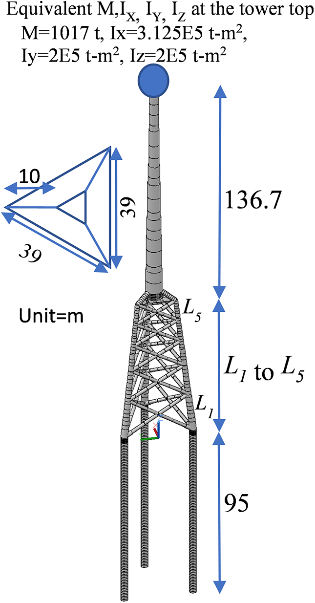
Figure 1: The tested OWT jacket support structures for the water depth of 70 m (L1 = 22 m, L2 = 18 m, L3 = 15 m, L4 = 13 m, and L5 = 12 m)

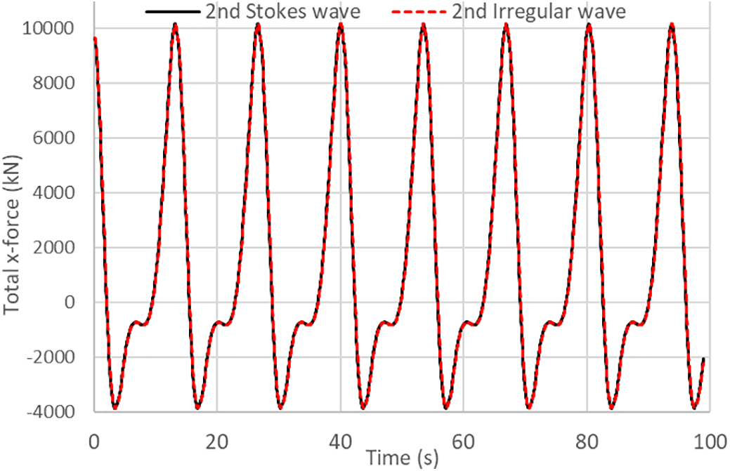
Figure 2: Comparison of time-history total wave x-direction forces between the second-order Stokes and second-order irregular wave theories under a single wave with a period of 12.798 s, wave height of 8.980 m, and wave length of 164.463 m at a water depth of 20 m

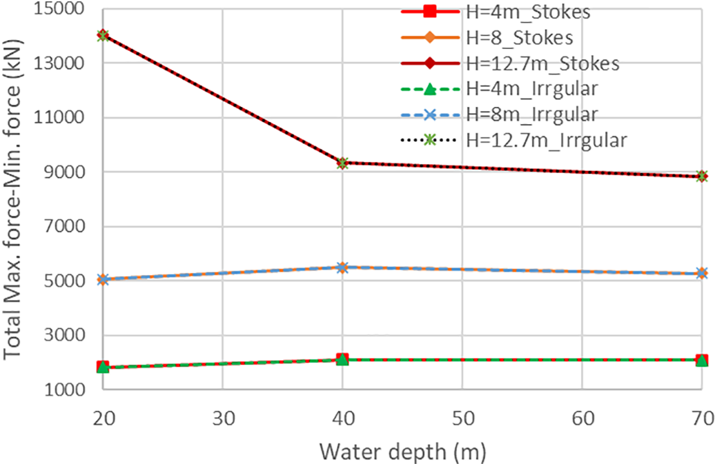
Figure 3: The variation between the maximum and minimum total wave loads from all the elements below the transient wave surface during a time-history analysis for all cases

3  Problems of Traditional Efficient Schemes for Time-Domain Wave Loads

The frequency-domain method, employing the inverse FFT, is efficient. This is because the FFT terms of nodal wave loads, as presented in Section 2.1, only need to be calculated once, and the inverse FFT is subsequently employed to obtain all the time-history wave loads. Conversely, the time-domain method requires the computation of FFT terms at each time step. However, the frequency-domain method is applicable only for small-displacement finite element analysis, since the nodal coordinates x, y, and z in the equations of Section 2.1 must remain fixed for the inverse FFT to be valid. Therefore, for the wave loads of FOWT support structures with a large displacement effect, the time-domain method is the preferred choice. In this paper, the following traditional schemes were proposed to enhance the computational efficiency of the time-domain method:

(1) Eliminating high-frequency terms

The second order model has demonstrated a good fit to experimental data when a cut-off frequency (fcut−off) equal to 2g/Hs/2π is applied [58]. This criterion was empirical rather than theoretical, and the recommended practice from Det Norske Veritas (DNV) [58] suggests this cut-off frequency equal to 4 times the spectral peak frequency. Despite its empirical nature, employing a cut-off frequency can significantly reduce the computational cost of second-order irregular wave loads. For example, if Nt2 is set to 8192 with fcut−off=2g/Hs/2π, the number of required frequencies is only 264. Consequently, the second-order irregular wave load calculation can be significantly accelerated, approximately (8192/264)2 = 963 times.

(2) Employing buffers to store the calculation results independent of x, y, and z coordinates

From the equations in Section 2.1, one can clearly understand the variable dependence. Variables with i and j are contingent on frequencies, those with m and n depend on wave direction, and the bolded equations with x, y, and z are linked to nodal coordinates. Variables independent of coordinates can be computed once and stored in a buffer for all the nodes and time steps. Subsequently, for each time step, the coordinate-dependent variables are calculated to determine those FFT parameters. For example, Eq. (28) can be modified to:

al=∑l=1NbufferE(imjn)lcosh⁡kimjn−(d+z)cos⁡(rp−ijnm)

where E(imjn)l=gs8[cicjDnDm1cosh⁡kimjn−d⋅Dimjn−(2π/Ti−2π/Tj)(kimx−kjnx)]l, and Nbuffer is the total number of iterations for i−j=l and i≥j under l=1 to Nt2. It is noted that variables E(imjn)l are computed only once for all the nodes and time steps.

(3) Parallel computation of element wave forces

The equations presented in Section 2.1 are not interdependent across distinct nodal coordinates, making parallel computation efficient at each node. Given that OWT structural analyses frequently demand the calculation of numerous nodal wave loads at each time step, complete parallelization proves to be highly efficient.

(4) Extrapolation of element wave forces over a defined number of time steps (Nextra)

Although wave loads are low-frequency, the time step length must still be sufficiently small to accommodate other types of loads. Therefore, an alternative is the extrapolation of wave loads over a certain number of time steps (Nextra), providing a balance between computational efficiency and accuracy. In this study, a quadratic exploitation using the wave loads from the three previous time steps was employed to determine the current wave loads for the next time step. For example, with two extrapolations and a calculation, the data from time steps n, n + 3, and n + 6 are used to extrapolate the data for steps n + 7 and n + 8, after which the data for step n + 9 is subsequently calculated.

Schemes (1) and (2) are essential procedures, and this study will exclusively examine the efficiency of schemes (3) and (4) by using a FOWT support structure. A semi-submersible platform was selected for this investigation because it features a high number of structural degrees of freedom and nodes, which leads to a heavier computational burden. This characteristic makes it an ideal case to highlight the benefits of the proposed acceleration techniques. In Fig. 4, the setup employed for this investigation involves the integration of the IEA 15 MW wind turbine [59] onto a DeepCwind semi-submersible platform [60] with four columns, positioned in waters with a depth of 100 m. The central column provides support for the tower, while the remaining three floating columns contribute additional stability. Structural integrity is preserved by interconnecting the pontoons through a system of 15 braces. To model the columns and braces, two-node Timoshenko beam elements were employed. These elements encompass functions that represent the floating stiffness at the sea surface, water-effective mass, and the load on the floating element. Key dimensions of both the tower and platform are specified in Fig. 4. A loading condition of IEC 61400-3-1 [61] Design Load Cases (DLC) 6.2 (parked (standing still or idling)) was employed, including a significant wave height (Hs) of 10 m, a wave direction from the X-axis (θwave) at 30 degrees, an average hub wind speed (Vhub) of 57 m/s, wind direction from the X-axis (θwind) at 30 degrees, and a misalignment of the yaw system (θyaw) at 90 degrees. These directions are illustrated in Fig. 4. The Newmark’s integration method was employed to conduct the large-displacement dynamic finite element analysis, utilizing a time step length of 0.05 s and a total time of 700 s. The following two ratios were defined to assess accuracy and CPU time under various conditions.

Accuracy ratio=∑k=1all time steps|Fk(Nextra=1)−Fk|/∑k=1all time steps|Fk(Nextra=1)|(38)

CPU ratio =CPU time of current condition/CPU time with Nextra=1and all CPU threads(39)

where Fk is the x-direction total wave force from all the members at time step k.

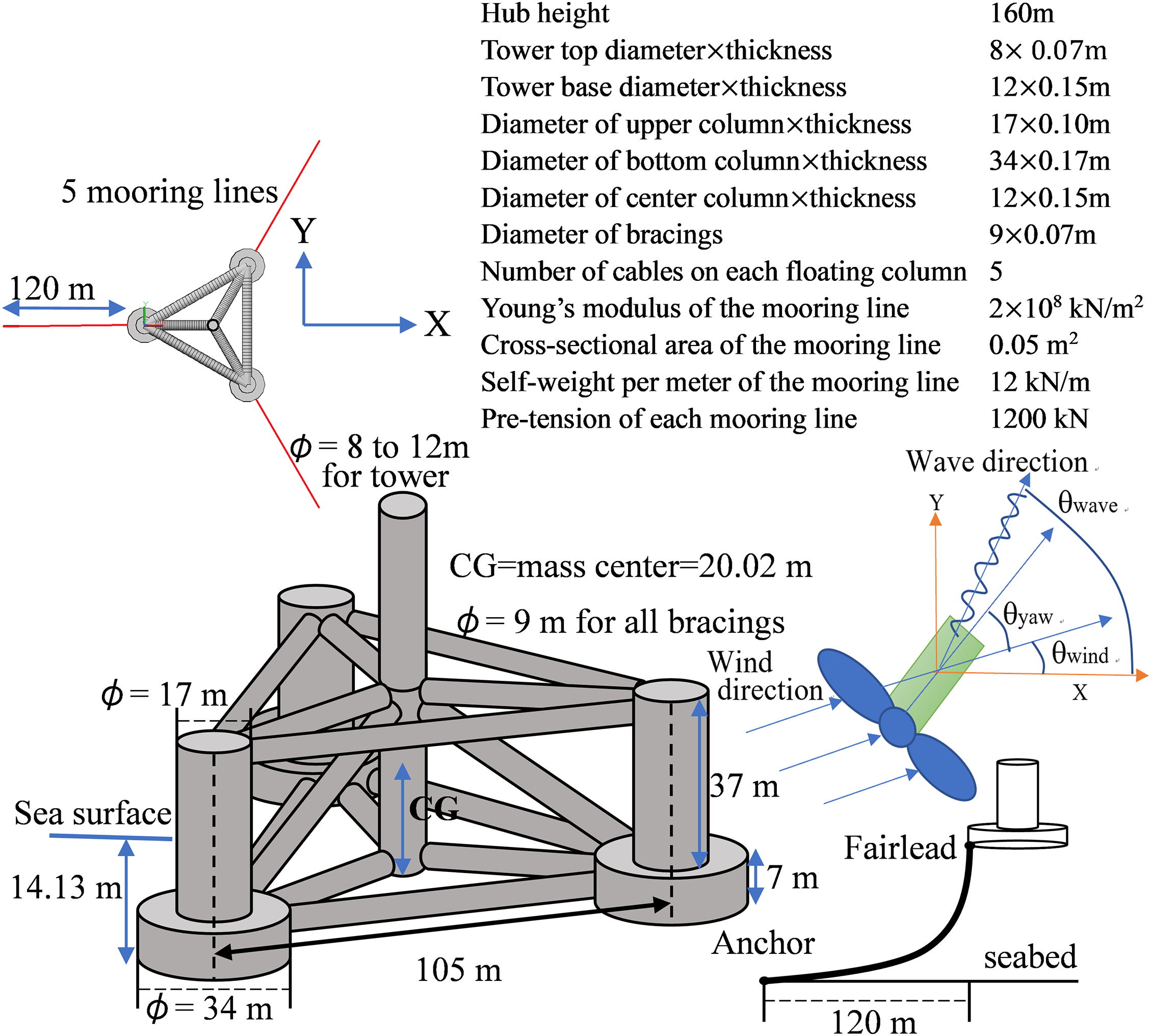
Figure 4: The dimensions and information of the 15 MW FOWT support structure in a water depth of 100 m (Vhub = 57 m/s, θwave = 30°, θwind = 30°, and θyaw = 90°)

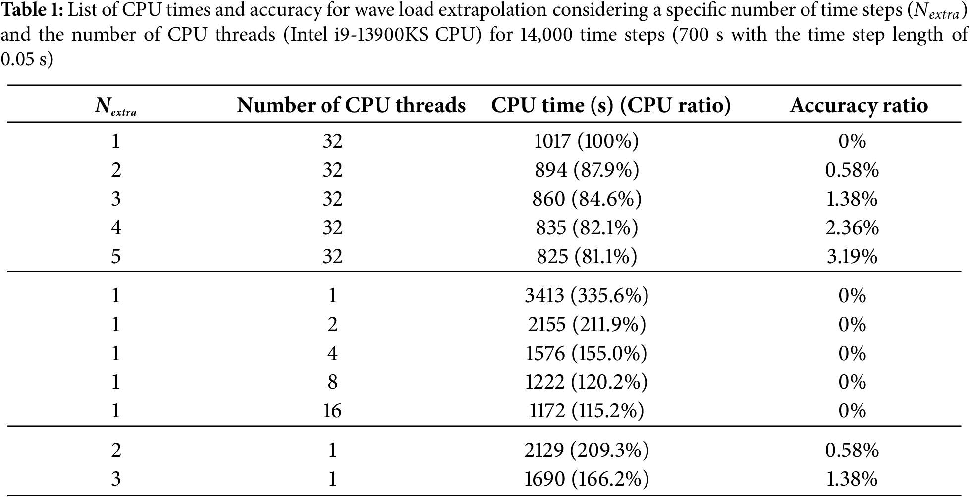
The values of these two ratios under various conditions are presented in Table 1, illustrating the following characteristics:

(1)   Regarding parallel computing, the number of CPU threads presented in Table 1 is only specified for wave load calculations, with other components being fully parallelized across all CPU threads. The efficiency of parallel computing is evident from Table 1, demonstrating that a threefold speedup can be achieved on a personal computer. Additionally, the table highlights that the computation of wave loads constitutes a significant portion of the CPU time, underscoring the necessity of parallel computation. The parallel procedure executed during nodal wave load calculation is the most effective approach.

(2)   When parallel computing is employed, the extrapolation of wave loads (Nextra > 1) is not as efficient. This is because a significant portion of wave load calculation has already been executed in parallel computing. However, in the absence of parallel computing, extrapolation for Nextra equal to two or three proves quite efficient without significantly compromising accuracy. This condition becomes beneficial when many loading cases must be analyzed. Given that the primary parallel computing is allocated to different finite element analyses with distinct loading cases, and possibly only one or several CPU threads are assigned to the wave load calculation, using Nextra equal to two or three is advantageous.

(3)   In OWT structural analyses, specifications such as IEC 61400-3, often recommend more than ten to twenty design load cases (DLCs), which may result in thousands of different loads. Additionally, for FOWT cases, the total time of finite element analyses is suggested to equal 3600 s. Therefore, based on the CPU time presented in Table 1, there is a need for further improvement in the computational efficiency of wave loads, especially for extended simulation durations, such as 3600 s. This is attributed to the fact that a prolonged simulation time requires significantly more CPU time for second-order wave calculation, and a topic will be explored in the subsequent section.

4  Continuous Formulations with Different Random Numbers

4.1 Formulations

Based on the numerical tests conducted in Section 3, the computational time for second-order wave loads remains excessively high. This issue would be exacerbated if an extended simulation time is necessary, such as 1000 s or more, given that the calculation process for second-order wave loads is roughly proportional to the square of Nt in Eq. (1). An alternative approach is to employ multiple FFT segments with different random numbers, significantly reducing the computation of second-order wave loads. However, using different random numbers introduces discontinuity at the connection point between two FFT segments. Therefore, this paper suggests the following interpolation method for the random numbers (φ) of the two FFT segments.

φ=φ1+s2(φ2−φ12)/(S0/2)2)for s≤S02(40)

φ=φ2−((S0−s)2(φ2−φ12)(S0/2)2)for s≥S02(41)

where φ1 is a random number in the first segment, and φ2 is that in the second segment, s is the time equal to 0 at the beginning of the interpolation, and S0 is the total time of the interpolation interval. These two equations form a quadratic representation of random numbers, with the minimum interval on either side and the maximum interval in the middle. To assess the error of the interpolation interval, an FFT term of Eq. (2) is utilized, as follows:

(aj+bjic)exp⁡(2πfjt+(φj+Δφj))ic=(aj+bjic)exp⁡((2πfj+Δφj/t)t+φj)ic(42)

where Δφj is the incremental random number at time t for frequency fj. If the random number interpolation is applied to the first segment, the frequency error should arise from Δφj/t. Given that the function is periodic with a period of T = NtΔt, the minimum value should be Δφj/T for this error term Δφj/t. Hence, the optimal strategy to minimize the error is to perform the interpolation near the end of the first FFT segment. This choice ensures that the time, excluding the periodic part, approaches T as the maximum value. Conversely, if the interpolation is set near the beginning of the second FFT segment, the time, excluding the periodic part, will approach zero resulting in a significant error. This error represents a specific percentage of the total duration of each segment. Consequently, since every segment carries the same percentage error, increasing the number of segments does not significantly affect the average error. While enlarging T can decrease the error, it may compromise computational efficiency.

4.2 Explanation of Computational Efficiency

To determine irregular waves, the computational efficiency can be approximated in the following equation for the frequency-domain method, time-domain method, and time-domain with different random numbers.

Ce1=N(Log2N) for the frequency−domain method using Inverse FFT (IFFT),(43)

Ce2=N2 for the time−domain method, and(44)

Ce3=N¯2m for the time−domain method with different random numbers(45)

where m is the number of different random numbers used in the total simulation time, N is the total number of time steps required for FFT terms, N¯ is the total number of time steps required for FFT terms under the condition that the analysis was divided into m segments. As shown in Section 2, N¯ is equal to N in the first-order wave theory, but it is obvious that N¯ is definitely much smaller than N for the frequency summation and difference terms in the second-order wave theory.

Although the computation speed of the time-domain method with different random numbers may be slower than the frequency-domain method using IFFT, it offers a practical alternative for scenarios requiring time-domain analysis. For FOWT support structures, where large displacements render IFFT invalid, this method represents a significant advancement in efficiency. Additionally, without corrections, the traditional time-domain method’s computation time grows exponentially with simulation duration, leading to prohibitive computational costs. By mitigating this growth, the segmentation method ensures that extended simulations remain feasible within a reasonable time frame, which is not much more than the frequency-domain method. In our previous research [62], we developed a fully coupled aero-hydro-servo-elastic simulation framework that satisfies IEC 61400-3-1 [61] load combination requirements. In such implementations, the wave load module described in this paper is responsible for calculating hydrodynamic forces at each time step, which are applied to a finite element model. The structure is modeled with full nodal resolution, where each node possesses six degrees of freedom. After all external loads and are applied, the nodal displacements, velocities, and accelerations are computed using Newmark’s method. The updated nodal positions are then passed back to update external force modules, including wave loads, mooring line tensions, aerodynamic and control systems for the next time step. This iterative process highlights the necessity of improving wave force computation speed, which is the focus of the present study.

4.3 Case Study

Utilizing different Nt2 with distinct FFT segments generates different random numbers for the wave load calculation, resulting in varying wave shapes. Specifications such as IEC and DNVGL recommend using different random numbers for different DLCs. Therefore, this study compares the CPU time and the steel design results of the FOWT support structure, as shown in Fig. 4, under the irregular wave with the same condition of Section 3, but the total simulation time changes from 700 s to 3600 s. The steel design program utilizes API and DNV-RP-C202 [63] standards to ascertain the required thickness for each tubular section under the DLC mentioned in Section 3. Notably, DNV-RP-C202 addressing local and global shell buckling effects is suitable for sections with a Diameter/thickness ratio exceeding 120. Seven different cases were analyzed including:

case 1: The whole time of 3600 s with a random number,

case 2: Nt2 = 8192 (Nt time steps) to change the random number with S0 = 10 s,

case 3: Nt2 = 8192 (Nt time steps) to change the random number with S0 = 5 s,

case 4: Nt2 = 8192 (Nt time steps) to change the random number with S0 = 2.5 s,

case 5: Nt2 = 8192 (Nt time steps) to change the random number with S0 = 1 s.

The CPU time and the difference of the steel design are presented in Table 2, Fig. 5 illustrates the wave height for the entire simulation duration, Fig. 6 depicts a connection interval between two FFT segments for cases 2 to 5, and Fig. 7 shows the wave height of the applied Jonswap spectrum and the FFT results of cases in Table 2. These results reveal the following features:

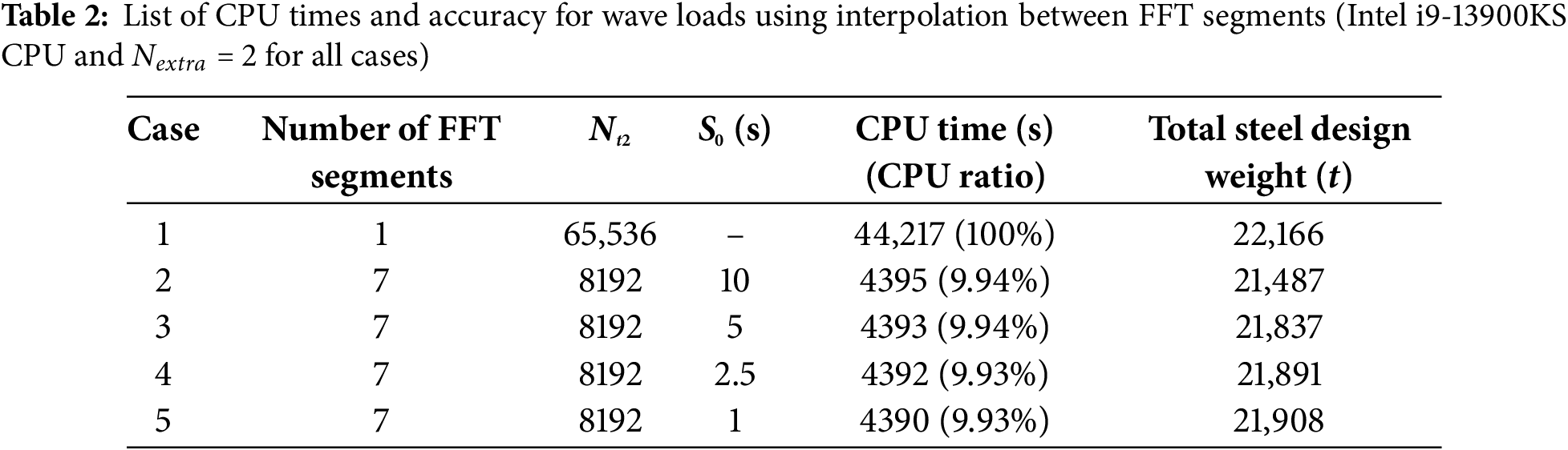
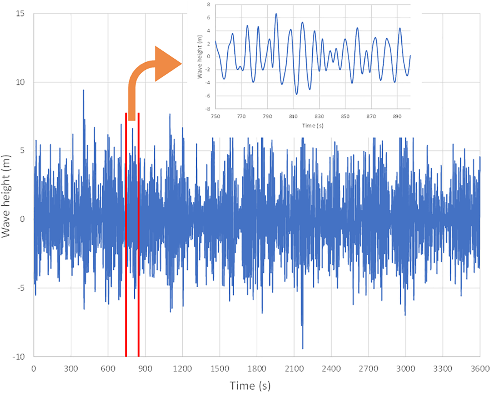
Figure 5: The complete wave height profile of Case 2 from the proposed time-domain wave equations with different random number segments

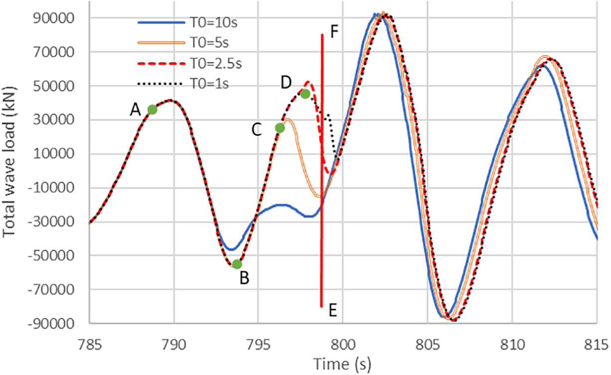
Figure 6: A connection interval between two FFT segment for cases 2 to 5 (S0 = 10 for point A, S0 = 5 for point B, S0 = 2.5 for point C, S0 = 1 for point D, and line EF = beginning of the 2nd segment)

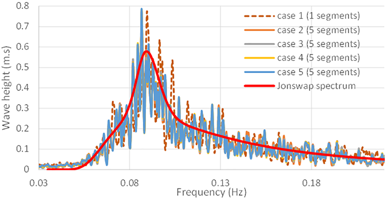
Figure 7: Wave height of the applied Jonswap spectrum and the converted wave height using FFT for the results of cases in Table 2

(1) The CPU times for FOWT structural analyses with Nt2 equal to 65,535 and 8192 differ by about ten times. This implies that employing an appropriate number of FFT segments with different random numbers can significantly reduce the computational load in second-order irregular wave calculations. Implementing this method, which utilizes different random numbers between two FFT segments, is not complex, as it only requires a simple subprogram using Eqs. (40) and (41) to modify a traditional wave load computer program.

(2) Design codes such as IEC and DNVGL require different random numbers for the wave load under various DLCs. Conducting numerous analyses and designs across these DLCs with a broad range of random number settings ensures that the design results are objective and reasonable. Table 2 illustrates that the maximum difference in total steel design weight is approximately 3.2% among these five cases, signifying that the proposed method with different random numbers between two FFT segments is practical.

(3) Fig. 5 demonstrates that the calculation using our proposed method and program results in a smooth line with no apparent interruption points. In Fig. 6, the connection curves between the first and second FFT regions are smooth, except for the case of T0 = 1 s, and we recommend setting T0 between 0.2Tp and Tp. This figure indicates that the beginning of the second FFT region is not at the same location, as the different wave loads at the connection lead to different displacements of the FOWT support structure. Notably, the FOWT support structure supported by mooring lines is sensitive to the wave load. Nevertheless, the proposed method can obtain smooth wave loads and significantly reduce CPU time.

(4) Fig. 7 illustrates the comparison between the applied Jonswap spectrum and the FFT frequency results for the five cases listed in Table 2, demonstrating acceptable accuracy. Cases 2 through 5 share the same set of random numbers, differing only in the connection time between the two segments, resulting in highly similar FFT outcomes. In contrast, Case 1 utilizes a different set of random numbers, leading to slight variations in its FFT results compared to Cases 2 to 5. Nevertheless, all cases exhibit sufficient accuracy when compared to the Jonswap spectrum.

(5) To further validate the efficiency of the proposed method, the total time of cases 1 and 2 changes from 3600 s to 700, 1800, 4800, and 7200 s. Moreover, the frequency domain method was also performed to be compared, although the method is not suitable for large-displacement analyses. Fig. 8 shows the CPU times for those cases. This outcome indicates that the required CPU time of the proposed method is still proportional to the total simulation time, if the used sub-region (8192 time steps for this example) does not change. Furthermore, the CPU time is not much larger than that of the frequency-domain method. However, that of the traditional time-domain wave method increases exponentially with the simulation time.

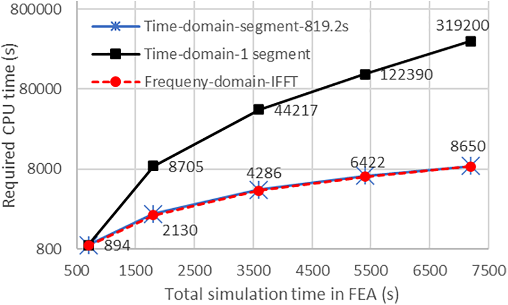
Figure 8: Comparisons of the required CPU time between the frequency-domain wave method and the time-domain wave method with and without different random numbers

5  Conclusions

This study collected and presented the explicit FFT parameters for second-order irregular wave height and loads from the research results of Sharma and Dean and applied them to both frequency-domain and time-domain methods. Given that FOWT support structures experience significant displacement effects under wave loads, the time-domain wave method becomes suitable for this problem. However, the time-domain method entails higher CPU time requirements than the frequency-domain method. To address this issue, the paper employs several numerical schemes, including efficient parallel computing and the extrapolation of element wave forces during specific time steps. While those schemes prove effective, the computational challenges persist due to the CPU time requirements in the time-domain wave method. Therefore, this study proposes a straightforward approach utilizing different random numbers in distinct FFT segments, aiming to significantly reduce the computation of second-order wave loads. Furthermore, this random number interpolation facilitates the creation of a continuous curve between two FFT segments. The paper also recommends interpolating near the end of the first FFT segment to minimize errors. Numerical studies demonstrate a significant reduction in the CPU times of FOWT structural analyses through the proposed method. Moreover, the steel design results do not vary excessively. Implementing this method, which involves using different random numbers between two FFT segments, is not complicated, as it only requires a simple subprogram using Eqs. (40) and (41) to modify a traditional wave load computer program. Furthermore, the proposed scheme can be used for time-domain methods for any physical problem that is not suitable for the use of IFFT. While the method was demonstrated using a semi-submersible platform with high structural complexity, it is also applicable to other FOWT support structures. However, the efficiency of the proposed extrapolation and segmentation techniques may be influenced by the specific dynamic behaviors and structural layouts of different platforms, and this warrants further study. Despite the advantages of the proposed method, several limitations should be noted. First, the time-domain wave load calculation remains computationally more expensive than frequency-domain approaches using IFFT, particularly for large-scale simulations. Second, although dividing the simulation into multiple FFT segments with interpolated random numbers can significantly reduce computation time, each segment still requires a non-trivial amount of computation. If the number of time steps per segment is too large, the efficiency gain diminishes. In this study, a segment size of 16,384 time steps was found to be a suitable balance between accuracy and computational cost. In addition, future extensions of this work may consider incorporating wave–structure interactions among multiple FOWTs in wind farms, which would allow further evaluation of the method’s scalability and applicability to cluster-level simulations.

Acknowledgement: Not applicable.

Funding Statement: This research was funded by National Science and Technology Council, grant number NSTC 113-2223-E-006-014.

Author Contributions: Conceptualization, Shen-Haw Ju; methodology, Shen-Haw Ju; software, Shen-Haw Ju; validation, Shen-Haw Ju, Yi-Chen Huang; formal analysis, Shen-Haw Ju; investigation, Shen-Haw Ju; resources, Shen-Haw Ju; data curation, Shen-Haw Ju; writing—original draft preparation, Shen-Haw Ju; writing—review and editing, Yi-Chen Huang; visualization, Shen-Haw Ju; supervision, Shen-Haw Ju; project administration, Shen-Haw Ju; funding acquisition, Shen-Haw Ju. All authors reviewed the results and approved the final version of the manuscript.

Availability of Data and Materials: The procedures and theories of this paper have been designed into computer programs, where the source codes can be obtained from “16. Wind turbine programs” in [https://sites.google.com/view/jushenhaw (accessed on 01 August 2025)], in which subroutines WAVEF, WAVEF0, IRWAVE, and IRWAVETM in file NBEAM.FOR are developed for the theories of the 2nd-to-15th stream function, Stokes 2nd, frequency-domain irregular wave, and time-domain irregular wave. The data that support the findings of this study are available from the Corresponding Author, [Shen-Haw Ju], upon reasonable request.

Ethics Approval: Not applicable.

Conflicts of Interest: The authors declare no conflicts of interest to report regarding the present study.

Nomenclature

Appendix A

FFT parameters of wave velocities and accelerations

For the first-order wave y-direction velocity, the FFT parameters are:

ai=πHiTicosh⁡ki(d+z)sinh⁡kid∑m=1NmDmsin⁡(θm)cos(rpim)(A1)

bi=−πHiTicosh⁡ki(d+z)sinh⁡kid∑m=1NmDmsin⁡(θm)sin(rpim)(A2)

For the first-order wave y-direction acceleration, the FFT parameters are:

ai=2π2HiTi2cosh⁡ki(d+z)sinh⁡kid∑m=1NmDmsin⁡(θm)sin(rpim)(A3)

bi=2π2HiTi2cosh⁡ki(d+z)sinh⁡kid∑m=1NmDmsin⁡(θm)cos(rpim)(A4)

For the first-order wave z-direction velocity, the FFT parameters are:

ai=πHiTisinh⁡ki(d+z)sinh⁡kid∑m=1NmDmsin(rpim)(A5)

bi=πHiTisinh⁡ki(d+z)sinh⁡kid∑m=1NmDmcos(rpim)(A6)

For the first-order wave z-direction acceleration, the FFT parameters are:

ai=−2π2HiTi2sinh⁡ki(d+z)sinh⁡kid∑m=1NmDmcos(rpim)(A7)

bi=2π2HiTi2sinh⁡ki(d+z)sinh⁡kid∑m=1NmDmsin(rpim)(A8)

FFT parameters of wave velocities and accelerations

(1) For frequency difference terms of the y-direction velocity:

al=gs8∑For i−j=lNt2cicj∑n=1NmDn∑m=1NmDmcosh⁡kimjn−(d+z)cosh⁡kimjn−d⋅Dimjn−(2π/Ti−2π/Tj)(kimy−kjny)cos⁡(rp−ijnm)(A9)

bl=−gs8∑For i−j=lNt2cicj∑n=1NmDn∑m=1NmDmcosh⁡kimjn−(d+z)cosh⁡kimjn−d⋅Dimjn−(2π/Ti−2π/Tj)(kimy−kjny)sin⁡(rp−ijnm)(A10)

where cp=gHpTp4π.(A11)

(2) For frequency summation terms of the y-direction velocity:

al=gs8∑For i−j=lNt2cicj∑n=1NmDn∑m=1NmDmcosh⁡kimjn+(d+z)cosh⁡kimjn+d⋅Dimjn+(2π/Ti+2π/Tj)(kimy+kjny)cos⁡(rp+ijnm)(A12)

bl=−gs8∑For i−j=lNt2cicj∑n=1NmDn∑m=1NmDmcosh⁡kimjn+(d+z)cosh⁡kimjn+d⋅Dimjn+(2π/Ti+2π/Tj)(kimy+kjny)sin⁡(rp+ijnm)(A13)

(3) For frequency difference terms of the y-direction acceleration:

al=gs8∑For i−j=lNt2cicj∑n=1NmDn∑m=1NmDmcosh⁡kimjn−(d+z)cosh⁡kimjn−d⋅Dimjn−(kimy−kjny)sin⁡(rp−ijnm)(A14)

bl=gs8∑For i−j=lNt2cicj∑n=1NmDn∑m=1NmDmcosh⁡kimjn−(d+z)cosh⁡kimjn−d⋅Dimjn−(kimy−kjny)cos⁡(rp−ijnm)(A15)

(4) For frequency summation terms of the y-direction acceleration:

al=gs8∑For i−j=lNt2cicj∑n=1NmDn∑m=1NmDmcosh⁡kimjn+(d+z)cosh⁡kimjn+d⋅Dimjn+(kimy+kjny)sin⁡(rp+ijnm)(A16)

bl=gs8∑For i−j=lNt2cicj∑n=1NmDn∑m=1NmDmcosh⁡kimjn+(d+z)cosh⁡kimjn+d⋅Dimjn+(kimy+kjny)cos⁡(rp+ijnm)(A17)

(5) For frequency difference terms of the z-direction velocity:

al=gs8∑For i−j=lNt2cicj∑n=1NmDn∑m=1NmDmsinh⁡kimjn−(d+z)cosh⁡kimjn−d⋅Dimjn−(2π/Ti−2π/Tj)sin⁡(rp−ijnm)kimjn−(A18)

bl=gs8∑For i−j=lNt2cicj∑n=1NmDn∑m=1NmDmsinh⁡kimjn−(d+z)cosh⁡kimjn−d⋅Dimjn−(2π/Ti−2π/Tj)cos⁡(rp−ijnm)kimjn−(A19)

where cp=πHpkpTp.(A20)

(6) For frequency summation terms of the z-direction velocity:

al=gs8∑For i−j=lNt2cicj∑n=1NmDn∑m=1NmDmsinh⁡kimjn+(d+z)cosh⁡kimjn+d⋅Dimjn+(2π/Ti+2π/Tj)sin⁡(rp+ijnm)kimjn+(A21)

bl=gs8∑For i−j=lNt2cicj∑n=1NmDn∑m=1NmDmsinh⁡kimjn+(d+z)cosh⁡kimjn+d⋅Dimjn+(2π/Ti+2π/Tj)cos⁡(rp+ijnm)kimjn+(A22)

(7) For frequency difference terms of the z-direction acceleration:

al=−gs8∑For i−j=lNt2cicj∑n=1NmDn∑m=1NmDmsinh⁡kimjn−(d+z)cosh⁡kimjn−d⋅Dimjn−cos⁡(rp−ijnm)kimjn−(A23)

References

1. Longuet-Higgins MS. Resonant interactions between two trains of gravity waves. J Fluid Mech. 1962;12(3):321–32. doi:10.1017/S0022112062000233. [Google Scholar] [CrossRef]
2. Dalzell J. A note on finite depth second-order wave–wave interactions. Appl Ocean Res. 1999;21(3):105–11. doi:10.1016/S0141-1187(99)00008-5. [Google Scholar] [CrossRef]
3. Johannessen TB, Swan C. A laboratory study of the focusing of transient and directionally spread surface water waves. Proc R Soc A-Math Phys Eng Sci. 2001;457(2008):971–1006. doi:10.1098/rspa.2000.0702. [Google Scholar] [CrossRef]
4. Longuethiggins MS, Stewart RW. Changes in the form of short gravity waves on long waves and tidal currents. J Fluid Mech. 1960;8(4):565–83. doi:10.1017/s0022112060000803. [Google Scholar] [CrossRef]
5. Stansberg C. Second-order numerical reconstruction of laboratory generated random waves. In: Proceedings of the 12th International Conference on Offshore Mechanics and Arctic Engineering; 1993 Jun 20–24; Scotland, UK. 143 p. [Google Scholar]
6. Bateman WJD, Swan C, Taylor PH. On the efficient numerical simulation of directionally spread surface water waves. J Comput Phys. 2001;174(1):277–305. doi:10.1006/jcph.2001.6906. [Google Scholar] [CrossRef]
7. Stansberg CT, editor. Non-Gaussian extremes in numerically generated second-order random waves on deep water. In: Proceedings of the ISOPE International Ocean and Polar Engineering Conference; 1998 Jul 26–31; Montreal, QC, Canada. Cupertino, CA, USA: ISOPE; 1998. [Google Scholar]
8. Zheng XY, Moan T, Quek ST. Non-Gaussian random wave simulation by two-dimensional Fourier transform and linear oscillator response to Morison force. J Offshore Mech Arct Eng. 2007;129(4):327–34. doi:10.1115/1.2783888. [Google Scholar] [CrossRef]
9. Zheng XY, Moan T, editors. Freak waves within the third order model. In: Proceedings of the International Conference on Offshore Mechanics and Arctic Engineering; 2010 Jun 6–11; Shanghai, China. p. 269–74. doi:10.1115/OMAE2010-20455. [Google Scholar] [CrossRef]
10. Lee C. Theory manual. Cambridge, MA, USA: Massachusetts Institute of Tech; 1995. [Google Scholar]
11. Sharma J, Dean R. Second-order directional seas and associated wave forces. Soc Pet Eng J. 1981;21(1):129–40. doi:10.2118/8584-PA. [Google Scholar] [CrossRef]
12. Forristall GZ. Wave crest distributions: observations and second-order theory. J Phys Oceanogr. 2000;30(8):1931–43. doi:10.1175/1520-0485(2000)030. [Google Scholar] [CrossRef]
13. Tromans PS, Vanderschuren L. A spectral response surface method for calculating crest elevation statistics. J Offshore Mech Arct Eng. 2004;126(1):51–3. doi:10.1115/1.1641390. [Google Scholar] [CrossRef]
14. Toffoli A, Onorato M, Babanin AV, Bitner-Gregersen E, Osborne AR, Monbaliu J. Second-order theory and setup in surface gravity waves: a comparison with experimental data. J Phys Oceanogr. 2007;37(11):2726–39. doi:10.1175/2007jpo3634.1. [Google Scholar] [CrossRef]
15. Ju SH, Chiu CS, Hsu HH. Studying the settlement of OWT monopile foundations using a T-Z spring with the torsional effect. Processes. 2023;11(2):17. doi:10.3390/pr11020490. [Google Scholar] [CrossRef]
16. Ju S-H. Studying the mode shape participation factor of wave loads for offshore wind turbine structures. Eng Struct. 2024;310:118067. doi:10.1016/j.engstruct.2024.118067. [Google Scholar] [CrossRef]
17. Ju SH, Chiu CS, Huang YC. Comparing traditional and suction piles in steel design of wind turbine structures. J Constr Steel Res. 2025;224(6):11. doi:10.1016/j.jcsr.2024.109169. [Google Scholar] [CrossRef]
18. Bredmose H, Agnon Y, Madsen PA, Schäffer HA. Wave transformation models with exact second-order transfer. Eur J Mech B-Fluids. 2005;24(6):659–82. doi:10.1016/j.euromechflu.2005.05.001. [Google Scholar] [CrossRef]
19. Forristall GZ. Irregular wave kinematics from a kinematic boundary condition fit (KBCF). Appl Ocean Res. 1985;7(4):202–12. doi:10.1016/0141-1187(85)90027-6. [Google Scholar] [CrossRef]
20. Schäffer HA. Second-order wavemaker theory for irregular waves. Ocean Eng. 1996;23(1):47–88. doi:10.1016/0029-8018(95)00013-B. [Google Scholar] [CrossRef]
21. Wang JH, Yan S, Ma QW. An improved technique to generate rogue waves in random sea. Comput Model Eng Sci. 2015;106(4):263–89. doi:10.3970/cmes.2015.106.263. [Google Scholar] [CrossRef]
22. Xia J, Wang Z, Jensen JJ. Non-linear wave loads and ship responses by a time-domain strip theory. Mar Struct. 1998;11(3):101–23. doi:10.1016/S0951-8339(98)00008-2. [Google Scholar] [CrossRef]
23. Yang ZW, Liu SX, Bingham HB, Li JX. Second-order coupling of numerical and physical wave tanks for 2D irregular waves. Part II: experimental validation in two-dimensions. Coast Eng. 2014;92(C2):61–74. doi:10.1016/j.coastaleng.2014.05.012. [Google Scholar] [CrossRef]
24. Li CX. Numerical Investigation of a hybrid wave absorption method in 3D numerical wave tank. Comput Model Eng Sci. 2015;107(2):125–53. doi:10.3970/cmes.2015.107.125. [Google Scholar] [CrossRef]
25. Xu G, Hamouda AMS, Khoo BC. Time-domain simulation of second-order irregular wave diffraction based on a hybrid water wave radiation condition. Appl Math Model. 2016;40(7–8):4451–67. doi:10.1016/j.apm.2015.11.034. [Google Scholar] [CrossRef]
26. Chen XJ, Moan T, Fu SX, Cui WC. Second-order hydroelastic analysis of a floating plate in multidirectional irregular waves. Int J Non-Linear Mech. 2006;41(10):1206–18. doi:10.1016/j.ijnonlinmec.2006.12.003. [Google Scholar] [CrossRef]
27. Rainey R. Slender-body expressions for the wave load on offshore structures. Proc R Soc Lond Ser A Math Phys Sci. 1995;450(1939):391–416. doi:10.1098/rspa.1995.0091. [Google Scholar] [CrossRef]
28. Bredmose H, Pegalajar-Jurado A. Second-order monopile wave loads at linear cost. Coast Eng. 2021;170:11. doi:10.1016/j.coastaleng.2021.103952. [Google Scholar] [CrossRef]
29. Morison JR, Obrien MP, Johnson JW, Schaaf SA. The force exerted by surface waves on piles. Trans Am Inst Min Metall Eng. 1950;189(05):149–54. doi:10.2118/950149-g. [Google Scholar] [CrossRef]
30. Sarpkaya T, Isaacson M, Wehausen J. Mechanics of wave forces on offshore structures. J Appl Mech. 1982;49(2):466–7. doi:10.1115/1.3162189. [Google Scholar] [CrossRef]
31. Cao Q, Xiao LF, Guo XX, Liu MY. Second-order responses of a conceptual semi-submersible 10 MW wind turbine using full quadratic transfer functions. Renew Energy. 2020;153(3):653–68. doi:10.1016/j.renene.2020.02.030. [Google Scholar] [CrossRef]
32. Reig MA, Pegalajar-Jurado A, Mendikoa I, Petuya V, Bredmose H. Accelerated second-order hydrodynamic load calculation on semi-submersible floaters. Mar Struct. 2023;90:22. doi:10.1016/j.marstruc.2023.103430. [Google Scholar] [CrossRef]
33. JN N, editor. Second-order slowly varying forces on vessels in irregular waves. In: Proceedings of the International Symposium on Dynamics of Marine Vehicles and Structures in Waves; 1974; London, UK. [Google Scholar]
34. Zhang LX, Shi W, Karimirad M, Michailides C, Jiang ZY. Second-order hydrodynamic effects on the response of three semisubmersible floating offshore wind turbines. Ocean Eng. 2020;207(11):22. doi:10.1016/j.oceaneng.2020.107371. [Google Scholar] [CrossRef]
35. Jonkman JM, Buhl ML. FAST user’s guide. Golden, CO, USA: National renewable energy Laboratory; 2005. Report No. NREL/EL-500-38230. [Google Scholar]
36. Jonkman B, Mudafort R, Platt A, Branlard E, Sprague M, Jonkman J, et al. OpenFAST/openfast:openfast v3.1.0. Zenodo. 2022:10. doi:10.5281/zenodo.6324288. [Google Scholar] [CrossRef]
37. da Silva LSP, de Oliveira M, Cazzolato B, Sergiienko N, Amaral GA, Ding B. Statistical linearisation of a nonlinear floating offshore wind turbine under random waves and winds. Ocean Eng. 2022;261:15. doi:10.1016/j.oceaneng.2022.112033. [Google Scholar] [CrossRef]
38. Han DD, Wang WH, Li X, Su XH. Optimization design of multiple tuned mass dampers for semi-submersible floating wind turbine. Ocean Eng. 2022;264(2):20. doi:10.1016/j.oceaneng.2022.112536. [Google Scholar] [CrossRef]
39. Branlard E, Geisler J. A symbolic framework to obtain mid-fidelity models of flexible multibody systems with application to horizontal-axis wind turbines. Wind Energy Sci. 2022;7(6):2351–71. doi:10.5194/wes-7-2351-2022. [Google Scholar] [CrossRef]
40. Duarte T, Gueydon S, Jonkman J, Sarmento A, editors. Computation of wave loads under multidirectional sea states for floating offshore wind turbines. In: Proceedings of the ASME 2014 33rd International Conference on Ocean, Offshore and Arctic Engineering; 2014 Jun 8–13; San Francisco, CA, USA. V09BT09A023. doi:10.1115/omae2014-24148. [Google Scholar] [CrossRef]
41. Coulling AJ, Goupee AJ, Robertson AN, Jonkman JM, Dagher HJ. Validation of a FAST semi-submersible floating wind turbine numerical model with DeepCwind test data. J Renew Sustain Energy. 2013;5(2):29. doi:10.1063/1.4796197. [Google Scholar] [CrossRef]
42. Orcina L. OrcaFlex user manual: OrcaFlex version 10.2 c. Cumbria, UK: Orcina Ltd.; 2018. [Google Scholar]
43. Ansys I. AQWA reference manual. Canonsburg, PA, USA: Ansys, Inc.; 2015. [Google Scholar]
44. Ghafari HR, Ghassemi H, He GH. Numerical study of the Wavestar wave energy converter with multi-point-absorber around DeepCwind semisubmersible floating platform. Ocean Eng. 2021;232(2):17. doi:10.1016/j.oceaneng.2021.109177. [Google Scholar] [CrossRef]
45. Yang Y, Bashir M, Li C, Wang J. Investigation on mooring breakage effects of a 5 MW barge-type floating offshore wind turbine using F2A. Ocean Eng. 2021;233(1):18. doi:10.1016/j.oceaneng.2021.108887. [Google Scholar] [CrossRef]
46. Ren YJ, Venugopal V, Shi W. Dynamic analysis of a multi-column TLP floating offshore wind turbine with tendon failure scenarios. Ocean Eng. 2022;245(5):14. doi:10.1016/j.oceaneng.2021.110472. [Google Scholar] [CrossRef]
47. Yan XK, Chen CH, Yin G, Ong MC, Ma Y, Fan TH. Numerical investigations on nonlinear effects of catenary mooring systems for a 10-MW FOWT in shallow water. Ocean Eng. 2023;276(3):21. doi:10.1016/j.oceaneng.2023.114207. [Google Scholar] [CrossRef]
48. Tang HJ, Yao HC, Yang RY. Experimental and numerical study of a barge-type floating offshore wind turbine under a mooring line failure. Ocean Eng. 2023;278(4):11. doi:10.1016/j.oceaneng.2023.114411. [Google Scholar] [CrossRef]
49. Hallak TS, Soares CG, Sainz O, Hernandez S, Arevalo A. Hydrodynamic analysis of the wind-bos spar floating offshore wind turbine. J Mar Sci Eng. 2022;10(12):22. doi:10.3390/jmse10121824. [Google Scholar] [CrossRef]
50. Coulling AJ, Goupee AJ, Robertson AN, Jonkman JM, editors. Importance of second-order difference-frequency wave-diffraction forces in the validation of a fast semi-submersible floating wind turbine model. In: Proceedings of the International Conference on Offshore Mechanics and Arctic Engineering; 2013 Jun 9–14; Nantes, France. New York, NY, USA: American Society of Mechanical Engineers; 2013. V008T09A019. doi:10.1115/OMAE2013-10308. [Google Scholar] [CrossRef]
51. Duarte TM, Sarmento AJ, Jonkman JM, editors. Effects of second-order hydrodynamic forces on floating offshore wind turbines. In: Proceedings of the 32nd ASME Wind Energy Symposium; 2014 Jan 13–17; National Harbor, MD, USA. doi:10.2514/6.2014-0361. [Google Scholar] [CrossRef]
52. Mei X, Xiong M. Effects of second-order hydrodynamics on the dynamic responses and fatigue damage of a 15 MW floating offshore wind turbine. J Mar Sci Eng. 2021;9(11):21. doi:10.3390/jmse9111232. [Google Scholar] [CrossRef]
53. Li W, Lei Y, Zheng XY, Gao S, Zheng HD, Zhao SX. Nonlinear Low-frequency response of a floating offshore wind turbine integrated with a steel fish farming cage. IEEE J Ocean Eng. 2023;48(1):160–87. doi:10.1109/joe.2022.3201242. [Google Scholar] [CrossRef]
54. Ma Y, Hu ZQ, Xiao LF. Wind-wave induced dynamic response analysis for motions and mooring loads of a spar-type offshore floating wind turbine. J Hydrodyn. 2014;26(6):865–74. doi:10.1016/s1001-6058(14)60095-0. [Google Scholar] [CrossRef]
55. Ju SH, Huang YC, Huang YY. Study of optimal large-scale offshore wind turbines. Renew Energy. 2020;154(2):161–74. doi:10.1016/j.renene.2020.02.106. [Google Scholar] [CrossRef]
56. Marintek S. USFOS hydrodynamics: theory description of use verification. Trondheim, Norway: SINTEF Marintek; 2010. [Google Scholar]
57. Ju SH, Hsieh CH. Optimal wind turbine jacket structural design under ultimate loads using Powell’s method. Ocean Eng. 2022;262(9):9. doi:10.1016/j.oceaneng.2022.112271. [Google Scholar] [CrossRef]
58. Nestegård A, Ronæss M, Hagen Ø., Ronold KO, Bitner-Gregersen EM, editors. New DNV recommended practice DNV-RP-C205 on environmental conditions and environmental loads. In: Proceedings of the ISOPE International Ocean and Polar Engineering Conference; 2006 Jun 18–23; San Francisco, CA, USA. [Google Scholar]
59. Gaertner E, Rinker J, Sethuraman L, Zahle F, Anderson B, Barter G, et al. Definition of the IEA 15-megawatt offshore reference wind turbine. Golden, CO, USA: National Renewable Energy Lab (NREL); 2020. doi: 10.2172/1603478. [Google Scholar] [CrossRef]
60. Robertson A, Jonkman J, Masciola M, Song H, Goupee A, Coulling A, et al. Definition of the semisubmersible floating system for phase II of OC4. Golden, CO, USA: National Renewable Energy Lab (NREL); 2014. Report No. NREL/TP-5000-6060. doi:10.2172/1155123. [Google Scholar] [CrossRef]
61. IEC-61400-3-1. Wind Turbines-part 3-1, Design requirements for fixed offshore wind turbines. Geneva, Switzerland: IEC; 2019. [Google Scholar]
62. Ju SH, Huang YC. Study on multiple wind turbines in a platform under extreme waves and wind loads. Energy Conv Manag X. 2025;25:11. doi:10.1016/j.ecmx.2025.100877. [Google Scholar] [CrossRef]
63. Veritas DN. Buckling strength of shells. In: Recommended practice RP-C202. Høvik, Norway: Det Norske Veritas; 2002. p. 1–21. [Google Scholar]
Cite This Article
Copyright © 2025 The Author(s). Published by Tech Science Press.
This work is licensed under a Creative Commons Attribution 4.0 International License , which permits unrestricted use, distribution, and reproduction in any medium, provided the original work is properly cited.
Downloads
Citation Tools