A Novel Multi-Objective Topology Optimization Method for Stiffness and Strength-Constrained Design Using the SIMP Approach

1  Introduction

Topology optimization (TO) [1–3] is a powerful computational tool for determining the optimal material distribution within a specified design domain. Since the pioneering work of the homogenization method, TO has become a fundamental technique in structural conceptual design. Over the years, diverse TO methodologies have been developed, including solid isotropic material with penalization (SIMP) [4,5], level-set methods (LSM) [6–9], evolutionary structural optimization (ESO) [10–12], iso-geometric analysis (IGA) [13–15] and the moving morphable components (MMC) method [16–18].

Compared to compliance-based TO, stress-constrained TO remains a formidable challenge due to its inherently local nature and computational intensity. While maximizing structural stiffness or minimizing compliance has been extensively studied [19–21], these approaches do not inherently ensure sufficient strength and durability [22–24]. Consequently, stress-constrained TO is critical for practical engineering applications [25–28]. However, due to the large number of finite elements involved in optimization problems, stress evaluation is computationally expensive, making large-scale structural applications particularly challenging.

To mitigate computational complexity, stress aggregation functions such as the Kreisselmeier-Steinhauser (K-S) function [29] and p-norm function [30] have been widely adopted, allowing the transformation of numerous local stress constraints into a single global stress measure [25,26,31]. However, these aggregation functions introduce approximation errors that can hinder effective local stress control, leading to poor convergence [21,26]. To alleviate this, block aggregation strategies [21,32] have been introduced, where multiple global stress measures are employed, but the accuracy remains sensitive to the number of aggregated constraints. Another key issue is stress singularity, particularly in density-based methods. Stress relaxation techniques [33,34] such as qp-relaxation [35] have been developed to address this issue by penalizing intermediate density elements, improving numerical stability and convergence.

In recent years, stress-constrained TO methods incorporating aggregation functions and qp-relaxation have been extensively employed in mass minimization, compliance minimization, and multi-objective optimization. These approaches enhance structural stress uniformity, thereby improving strength and durability. Fan et al. [36] integrated stress constraints into ESO to address traditional TO limitations. Ferro et al. [37] explored compliance and stress constrained TO for mass minimization, demonstrating significant weight reduction while satisfying stress constraints. Ma et al. [38] incorporated qp-relaxation with sensitivity weighting and p-norm aggregation in a bidirectional evolutionary structural optimization (BESO) framework, enhancing computational efficiency and stability. Zhai et al. [39] introduced an augmented Lagrangian formulation where auxiliary stress variables were constrained by equality constraints, leading to improved solution effectiveness. Liu et al. [40] employed qp-relaxation and p-norm functions to enhance structural performance in additive manufacturing applications. Zheng et al. [41] further integrated p-norm stress aggregation with self-support constraints in thermoelastic structures. Additionally, Nguyen and Lee [42] were the first to achieve the optimization design of multi-material structures subjected to self-weight loads while considering stress constraints. Xia et al. [43,44] employed stress influence functions (SIF) to handle large-scale stress constraints, providing an efficient framework for addressing high-stress regions in structural optimization.

Despite the progress in stress constrained TO, achieving a balanced design that simultaneously considers both stiffness and strength remains a significant challenge. Stiffness is a global property, while stress is a local measure, making it difficult to directly integrate the two into a unified optimization framework. To address this issue, this paper proposes a novel topology optimization framework that achieves coordinated stiffness and stress-constrained optimization based on SIMP model. Numerical examples demonstrate the proposed method’s performance across various optimization models, indicating its capability to achieve lightweight structures. This research provides a robust theoretical foundation and practical insights for the optimization of complex engineering structures. The main contributions of this work are as follows:

(1)   A new objective function is formulated by integrating globalized stress constraints and structural stiffness using a normalized linear weighting strategy, allowing for a unified multi-objective optimization approach.

(2)   The proposed method employs the p-norm aggregation function to globalize local stress constraints, effectively reducing computational complexity while maintaining accurate stress control.

(3)   The implementation of density filtering and Heaviside projection within the SIMP framework ensures numerical stability and eliminates gray elements, improving the manufacturability of optimized designs.

The structure of this paper is as follows. Section 2 presents the problem statement. Section 3 introduces the TO algorithm framework incorporating stiffness and stress constraints. In Section 4, the proposed methods are validated using through two numerical cases. Finally, Section 5 presents the conclusions of this paper.

2  Problem Statement

2.1 SIMP Approach

The effective elastic modulus of structural elements is defined using the SIMP method, as expressed in Eq. (1).

E=(xi)pE0(1)

where E0 and E represent the pseudo-elastic moduli before and after optimization, respectively.

The element stiffness matrices ka0 and kae correspond to the pre- and post-optimized states, leading to the Eq. (2).

kae=(xi)pka0(2)

In the SIMP model, penalization factor p is introduced to suppress intermediate density elements. The primary objective of this penalization is to enforce a near 0–1 material distribution by discouraging intermediate values, thereby ensuring a well-defined topology and reducing manufacturing uncertainties.

2.2 Global Stress Measure

Aggregation functions can aggregate large amounts of stress values to a global stress measure which approximates the maximum stress value [14]. This global stress measure has adequate smoothness so that the optimization algorithm could perform well. p-norm function is used in this study.

σpn=(∑i=1Nσvm,ipn)1pn(3)

where σpn denotes the global stress measure and σvm,i denotes the von Mises stress at the centroid of the ith element. pn denotes the stress norm parameter. σpn approaches the average stress value when pn tends to one and approaches to the maximum stress value when pn tends to infinity. In the global stress measurement calculation, the parameter pn has a significant impact on the optimization result. Theoretically, the larger the value of pn, the better, as it can provide a more accurate approximation of the maximum stress, making it easier for the design result to meet the stress constraints. However, practical evidence shows that an excessively large pn value will increase the gradient of the sensitivity value within the design domain, thereby exacerbating the instability of the numerical calculation and ultimately leading to the inability to find the optimal solution. An appropriate stress norm parameter can balance the smoothness of the p-norm function and the approximation for the maximum stress value in the structure, pn = 8 in this study.

The von Mises stress can be expressed as Eq. (4).

σvm,i=(σiTTσi)0.5(4)

where σi denotes the stress vector of centroid of ith element. T is the stress coefficient matrix.

For plane stress case, σi=[σx,σy,σxy]T.

T=[1−0.50−0.510003](5)

2.3 Qp-Relaxation

To obtain a black-and-white design, a penalization function is introduced to penalize the intermediate density. For stress-based topology optimization problem, the penalization of stress for intermediate design variable values is described in Ref. [45]. The element stress can be expressed based on SIMP penalization function as shown in Eqs. (6) and (7).

σ^i=(xi)qσi(6)

σi=D0Biui=[σxσyσxy]T(7)

where σi is the stress matrix calculated at the center point of the element, containing 3 stress components; D0 is the elastic matrix of the solid material; Bi is the strain matrix; p=3, q=0.5 in this study.

2.4 Optimization Model

In conventional TO, the mathematical models are typically formulated based on the combination of three primary criteria: mass, stress, and compliance (strain energy). For specific engineering problems, additional objectives or constraints may be incorporated as needed. However, the present study does not focus on a particular application. The following provides a brief description of five mathematical models formulated using these three criteria.

Model Q1: Compliance minimization. Structural compliance is commonly represented by strain energy. Under the SIMP material interpolation model, when optimizing purely for structural rigidity, the objective function aims to minimize global compliance, subject to a material volume constraint, as shown in Eq. (8).

{find x={x1,x2,x3,⋯,xe}T∈RnminC(x)=UTKaU=∑e=1N(ue)Tkaeue=∑e=1N(xe)p(ue)Tka0ues.t.∑e=1Nxeve≤f⋅V0,KaU=Pa0<xmin≤xe≤xmax(8)

where C(x) represents the total structural compliance; Ka represents the global stiffness matrix; U represents the global displacement vector; ue represents the element nodal displacement vector. The variable xe represents the relative density of element e, with penalization factor p. The parameters V0 and ve represent the initial total volume and the volume of element e, respectively. The volume fraction constraint is defined by f, while xmin, xmax represent the lower and upper bounds of the element densities. The total number of elements in the discretized domain is N.

Model Q2: Global stress minimization. Structural strength is typically characterized by the maximum von Mises stress. In this study, a p-norm function is employed as an alternative to the maximum von Mises stress to enhance numerical stability. Under the SIMP framework, the optimization model for global stress minimization, subject to a material volume constraint, is formulated as shown in Eq. (9).

{findx={x1,x2,x3,⋯,xe}T∈Rnminσpn=(∑i=1Nσvm,ipn)1pns.t.∑e=1Nxeve≤f⋅V0,KaU=Pa0<xmin≤xe≤xmax(9)

where σvm,i represents the von Mises stress at the centroid of element i, and σvm,i=(σiTTσi)1/2; T represents the stress transformation matrix. The function σpn is the global stress function, while pn is the p-norm parameter. The design variable is x, and v represents the volume of element e.

Model Q3: Mass minimization with compliance and stress constraints. Under the SIMP material interpolation model, when minimizing the structural mass, the objective function aims to minimize the volume fraction while ensuring compliance and stress constraints, as shown in Eq. (10).

{findx={x1,x2,x3,⋯,xe}T∈RnminVs.t.KaU=PaσP≤σVMC≤Cmax0<xmin≤xe≤xmax(10)

Model Q4: Compliance minimization with mass and stress constraints. This model seeks to minimize global compliance while imposing constraints on the volume fraction and global stress, as shown in Eq. (11).

{findx={x1,x2,x3,⋯,xe}T∈RnminC(X)s.t.∑e=1Nxeve≤f⋅V0,KaU=PaσP≤σVM0<xmin≤xe≤xmax(11)

Model Q5: Global stress minimization with mass and compliance constraints. This model aims to minimize the global stress function while maintaining constraints on volume fraction and compliance, as shown in Eq. (12).

{findx={x1,x2,x3,⋯,xe}T∈Rnminσpn=(∑i=1Nσvm,ipn)1pns.t.∑e=1Nxeve≤f⋅V0,KaU=PaC≤CMAX0<xmin≤xe≤xmax(12)

3  Method

3.1 Mathematical Model for Stiffness-Strength Coordinated Optimization

To achieve a balance between structural stiffness and strength, a multi-objective optimization model is formulated. The proposed optimization model, denoted as Model Q6, integrates strain energy and global structural strength into a unified objective function. The optimization formulation is expressed as Eq. (13).

{findx={x1,x2,x3,⋯,xe}T∈RnminS(x)=w1C(x)C0max+(1−w1)σpnσvm,0maxs.t.∑e=1Nxeve≤f⋅V0,KaU=Pa0<xmin≤xe≤xmax(13)

where C(x) represents the total compliance of the structure, and σpn is the aggregated stress function. To ensure balanced contributions from both terms, normalization is applied using reference values C0max and σvm,0max, which are estimated from Initial calculation of the model. It should be noted that the grid size in all the optimized models should remain consistent to maintain the consistency of the initial reference values. If stress minimization is a major concern, a larger weighting factor is assigned to global stress function, i.e., w1=0.3. It is worth noting that by introducing an adaptive weight strategy, such as dynamically adjusting w1 based on the sensitivity of the objective function during the iterative process; not only can the dependence on prior weights be reduced, but it also helps to reveal the trade-off mechanism between different physical targets. However, this paper aims to verify the effectiveness and correctness of the proposed method, and did not adopt the adaptive weight strategy. Instead, it used the commonly used Pareto frontier analysis to achieve a balance between performance and robustness. The specific value of w1 needs to be determined based on Eq. (31) in Section 4.3 that follows.

A key parameter in Model Q6 is the weight coefficient 1≥wi≥0, which determines the relative importance of stiffness and strength in the optimization process. The coefficient satisfies Eq. (14).

∑i=1kwi=1(14)

when w1=1, the problem is reduced to a compliance minimization problem, focusing solely on maximizing stiffness. When w1=0, the optimization becomes a stress minimization problem, prioritizing structural strength. By varying w1, different Pareto-optimal topologies can be obtained, allowing for a tailored balance between stiffness and strength.

Since stiffness and strength are typically of different numerical magnitudes, direct summation in a multi-objective formulation may cause numerical imbalance. Therefore, in order to ensure meaningful optimization results, compliance normalization and aggregated stress normalization are necessary. The proposed model provides a flexible framework for achieving an optimal stiffness-strength trade-off, which is crucial for structural performance under real-world loading conditions.

3.2 Sensitivity Analysis

In TO, the sensitivity of design responses—including both objective functions and constraints—with respect to design variables must be determined to facilitate the optimization process. For Model Q6, the sensitivity of the weighted objective function S(x) in Eq. (13) with respect to the design variable xj is expressed as shown in Eq. (15).

∂S(x)∂xj=(w1C0max)∂C(x)∂xj+(1−w1σvm,0max)∂σpn∂xj(15)

In this hybrid weighted topology optimization model, the objective function comprises both the sensitivity term of structural compliance and that of global structural stress. Under static or quasi-static loading conditions, external forces remain constant. Based on the assumptions of the SIMP method, the sensitivity of structural compliance C(x) can be derived as Eq. (16).

∂C(x)∂xj=−∑1N(ue)T∂kae∂xjue=−p∑e=1N(xj)p−1(ue)Tka0ue(16)

The sensitivity equation for global stress aggregation function σpn is given by Eq. (17).

∂σpn∂xj=∂σq∂σvm,i(∂σvm,i∂σ^i)Tq(xi)q−1σi+∂σq∂σvm,i(∂σvm,i∂σ^i)T(xi)q∂σi∂xj(17)

Rewriting the equation in Eq. (18).

{∂σq∂xj=T1+T2T1=∑i=1N(∂σq∂σvm,i[(∂σvm,i∂σ^i)q(xi)q−1σi])T2=∑i=1N(∂σq∂σvm,i[(∂σvm,i∂σ^i)T(xi)q∂σi∂xj])(18)

where ∂σpn/∂σvm,i can be expressed as Eq. (19).

∂σpn∂σvm,i=(∑i=1N(σvm,i)pn)1pn−1(σvm,i)pn−1,(19)

Based on the von Mises stress definition in Eqs. (4) and (5), the derivative of the local element von Mises stress σvm,i with respect to the stress vector σi is given by Eq. (20).

{∂σvm,i∂σi,x=12σvm,i(2σi,x−σi,y)∂σvm,i∂σi,y=12σvm,i(2σi,y−σi,x)∂σvm,i∂τi,xy=3τi,xyσvm,i(20)

where ∂σi/∂xj can be expressed as Eq. (21).

∂σi∂xj=D0Bi∂ui∂xj=D0BiLi∂U∂xj(21)

where Li is a 0–1 sparse matrix to extract the nodal displacement of the ith element from the global displacement [U](ui=LiU); Note that material stiffness matrix D0 and the elemental strain matrix Bi are independent of the design variable xj.

Inserting Eq. (21) into the term T2 in Eq. (18), we can find T2 can be rewritten as Eq. (22).

T2=∑i=1N(∂σq∂σvm,i(∂σvm,i∂σ^i)T(xi)qD0BiLi∂U∂xj)(22)

The adjoint method is applied here to resolve the above equation. The term ∂U/∂xj can be obtained through differentiating both sides of the equilibrium Eq. (2) as Eq. (23).

∂K∂xjU+K∂U∂xj=0(23)

Therefore, the term T2 can be further written as Eq. (24).

T2=∑i=1N(−(xi)q∂σpn∂σvm,i(∂σvm,i∂σ^i)TD0BiLi)K−1∂K∂xjU(24)

An adjoint variable [λ] is now defined as Eq. (25).

λT=(∑i=1N(xi)q∂σPN∂σvm,i(∂σvm,i∂σ^i)TD0BiLi)K−1(25)

Therefore, adjoint variable λ can be calculated from the adjoint equation as Eq. (26).

Kλ=(∑i=1N(xi)q∂σpn∂σvm,i(D0BiLi)T∂σvm,i∂σ^i)(26)

Thus, the term T2 can be further simplified to Eq. (27).

T2=−λT∂K∂xjU(27)

The term ∂K/∂xj can be expressed as Eq. (28).

∂K∂xj=∑i=1NLiT∂kaj∂xjLi=LjT(p⋅xjp−1ka0)Lj(28)

3.3 Density Filtering and Projection

The optimization scheme based on the SIMP method has a mesh dependency problem, which leads to the optimization results appearing checkerboard phenomenon. This problem can be solved effectively by utilizing a density filter. The equation of the density filter is as follows:

x¯e=∑j∈Newe,jxj∑j∈Newe,j(29)

where xj and Ne are the other elements and the total number of elements located within a certain distance of element e, respectively.

And we,j is the weight coefficient, which is computed by the following equation:

we,j=(rmin−dist(e,j)),{j∈Ne|dist(e,j)≤rmin}(30)

where rmin is the filtering radius and dist(e,j) denotes the Euclidean distance between elements e and j.

Furthermore, to reduce the grayscale elements in the optimization results, we project the filtered density field using the Heaviside projection function [45]. The relative density of element e obtained with this function is as follows:

x^e=tanh⁡(βη)+tanh⁡(β(x¯e−η))tanh⁡(βη)+tanh⁡(β(1−η))(31)

where η and β are the threshold and steepness of the Heaviside function, respectively. The larger the value of β, the more effective removal of grayscale elements. However, larger value of β leads to deterioration of the convergence of the topology optimization. Herein, in this article, β is set to 8 and η is set to 0.5.

3.4 The Proposed Method

The flowchart of the proposed method for stiffness-strength coordinated design is shown in Fig. 1. This method includes the following steps:

STEP 1: Define the design domain, establish the finite element model, and assign a design variable (ranging from 0 to 1) to each element. Set boundary conditions, including support constraints and loading conditions. Define optimization parameters such as the sensitivity filter radius rmin and penalization factors p and q.

STEP 2: Perform interpolation of element stiffness and element stress using a combination of the SIMP method and the qp-relaxation approach.

STEP 3: Conduct finite element analysis (FEA) of the overall structure.

STEP 4: Extract displacement fields, element stiffness matrices, and von Mises stress data from the FEA results.

STEP 5: Compute strain energy and global equivalent stress based on the displacement fields, element stiffness matrices, and von Mises stress data obtained in STEP 4.

STEP 6: Formulate the optimization objective function by normalizing strain energy and global equivalent stress, followed by their weighted linear combination using a predefined weight coefficient. Different weight coefficients are selected to achieve the desired balance between stiffness and strength.

STEP 7: Apply the derived sensitivity filtering approach for compliance-stress hybrid sensitivity to mitigate numerical instability during the optimization process.

STEP 8: Update design variables iteratively using the MMA.

STEP 9: Repeat STEP 2–8 until convergence criteria are satisfied.

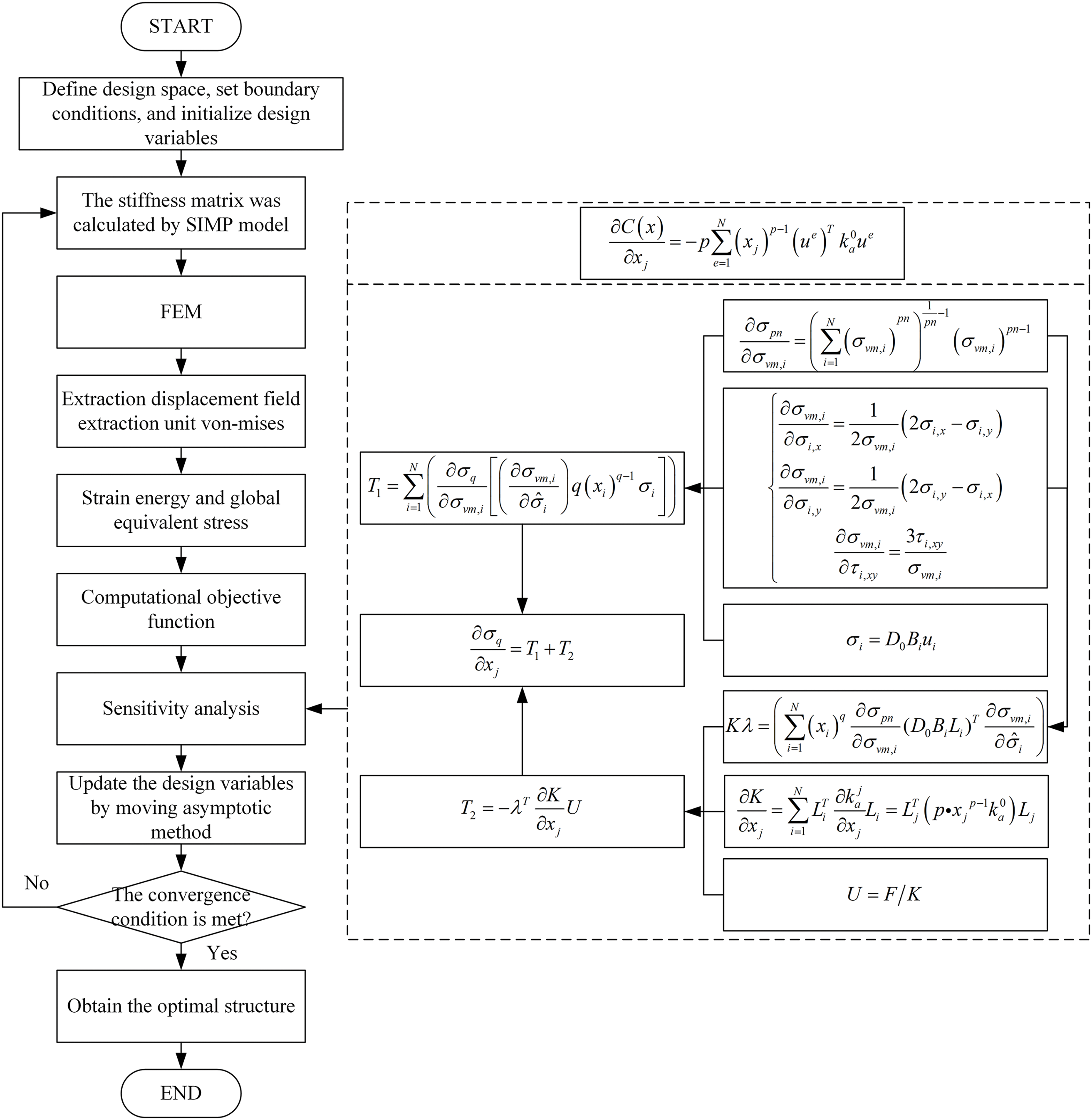
Figure 1: The flow chart of TO method incorporating stiffness and strength constraints

4  Numerical Examples

In two two-dimensional cases, the Young’s modulus is set to 1.0 MPa and the Poisson’s ratio to 0.3. In the final three-dimensional case, the Young’s modulus is set to 2×105 MPa and the Poisson’s ratio to 0.3. Unless otherwise specified, all dimensions and stress values in this study are expressed in millimeters (mm) and megapascals (MPa), respectively, with the results rounded to three decimal places. The topology optimization numerical calculations were conducted for three cases using the Q1–Q6 optimization models. For the Q6 model, the weight coefficient w1 was set at 0.2, 0.4, 0.6, and 0.8. A comparative analysis of the optimized results, focusing on mass, maximum strain energy, and maximum Von-Mises stress, is performed to validate the effectiveness of the proposed method.

Special Note: In this study, the computational tasks were completed on a high-performance personal computer. Its hardware configuration is as follows: The processor uses Intel Core i7-12800HX, featuring 16 cores and 24 threads, with a base frequency of 2 GHz. All the following cases were completed on the computer.

4.1 Messerschmitt-Bölkow-Blohm Beam (MBB) Design with One Pre-Existing Crack Notch

The first numerical case involves an MBB beam with a notch. The dimensions and boundary conditions are shown in Fig. 2. The beam has a thickness of 1.0 mm, and the design domain is discretized using 26,900 three-node plane stress elements, each with a size of 1.0 mm. The filtering radius, rmin, is set to 3.0 mm. A vertical force of F = 5 N is applied at the center of the top edge. To prevent stress concentration, the force is distributed over a 10 mm section at the midpoint of the beam’s top edge. The volume fraction is specified as 0.4. The maximum Von-Mises stress in the structure occurs at the notch of the beam, with a value of σvm,max = 2.42 MPa.

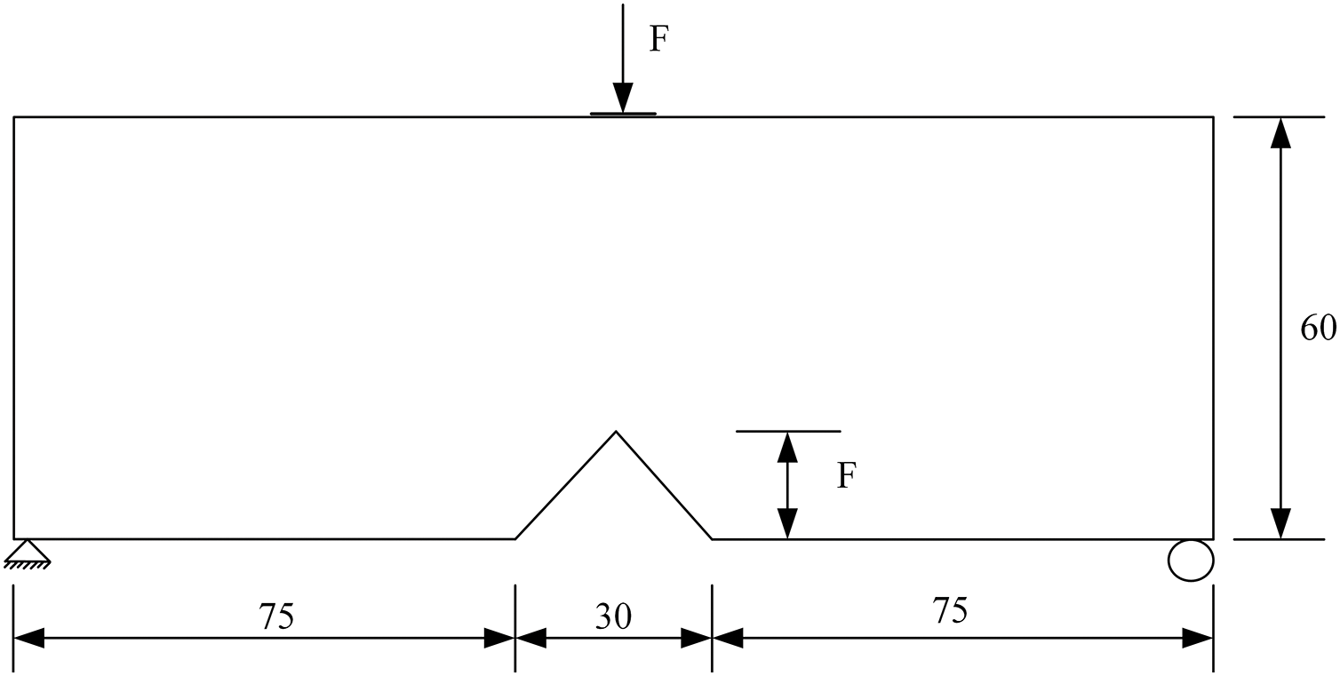
Figure 2: The dimensional schematic and boundary conditions of the MBB beam

Fig. 3 presents the topology optimization results for the MBB beam design with a pre-existing crack notch, obtained using six optimization models in this study. Fig. 3a shows the topology optimization result for the Q1 model, which minimizes compliance. Fig. 3b illustrates the topology optimization design for the Q2 model, focused on stress minimization. Fig. 3c displays the topology optimization result of the Q3 model, which minimizes compliance subject to a stress constraint. Fig. 3d presents the topology optimization design for the Q4 model, which minimizes stress under a compliance constraint. Fig. 3e shows the topology optimization result for the Q5 model, which minimizes mass while considering both stress and compliance constraints. Fig. 3f–i presents the structural stiffness-stress coordinated design results for the Q6 model, with weight coefficients w1 = 0.2, 0.4, 0.6, and 0.8.

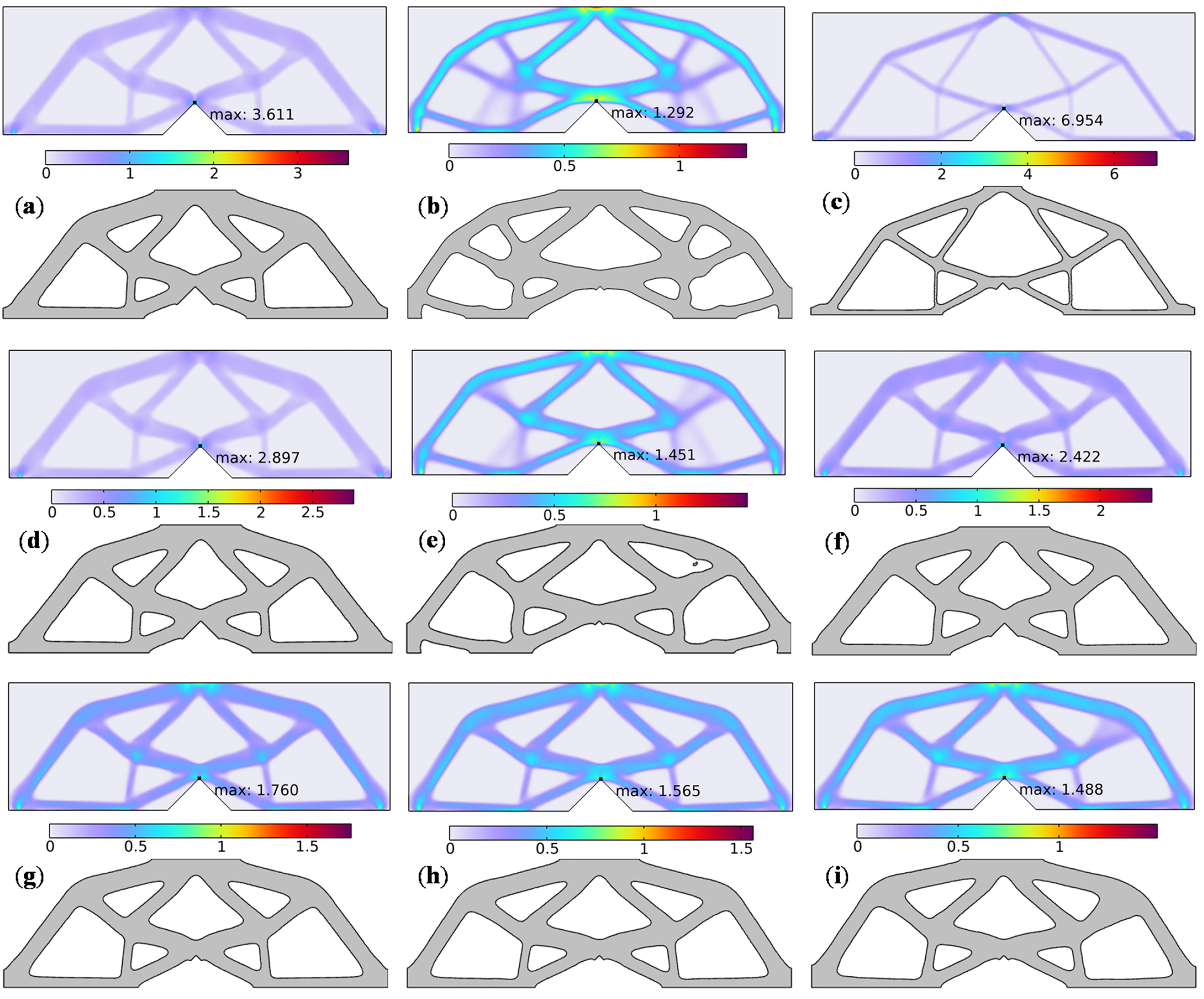
Figure 3: The result of MBB beam. (a) Q1; (b) Q2; (c) Q3; (d) Q4; (e) Q5; (f) Q6 when w1 = 0.2; (g) Q6 when w1 = 0.4; (h) Q6 when w1 = 0.6; (i) Q6 when w1 = 0.8

Fig. 3a,b shows similar topology structures in terms of mass and strain energy. However, the stress at the right-angle corner of the L-shaped bracket in Fig. 3a is approximately three times higher than that in Fig. 3b, indicating the significant effect of the aggregated function in minimizing structural stress.

The topological structure in Fig. 3d shows little difference from that in Fig. 3a in terms of mass and strain energy, while the maximum stress has decreased by approximately 0.8 MPa. This indicates that the stress constraints added in the Q4 model have played a role in reducing the maximum stress.

In Fig. 3e, its topological structure is different from that in Fig. 3b. This is because a flexibility constraint has been added. It can be observed that after applying the flexibility constraint, the strain energy has decreased by 0.013 J. This confirms that adding a flexibility constraint can increase the model’s stiffness.

Fig. 3c shows the topology with the smallest mass among all optimization models, approximately 12.355 g. However, both the strain energy and the maximum stress at the right-angle corner reach the highest values across all models. Furthermore, the constraint on the maximum stress at the notch of the MBB beam does not satisfy the requirement of being less than or equal to the maximum stress of the Q2 model, indicating that this constraint does not effectively couple the structural flexibility and strength. This approach may lead to excessively thin branches in the optimized topology. To avoid such fine branching structures, additional minimum size constraints are necessary, which may reduce computational efficiency and occasionally lead to convergence issues.

Fig. 3f–i shows that as the weight coefficient increases, the mass remains nearly constant, while the strain energy gradually increases with only slight variations. The maximum stress at the notch of the MBB beam decreases as the weight coefficient increases, with the most significant reduction occurring at w1 = 0.2 and w1 = 0.4. To better illustrate the coordination of stiffness and strength in the proposed method, the variation curves of strain energy and maximum Von-Mises stress across different weight coefficients are shown in Fig. 4. The optimization results for mass, strain energy, and maximum Von-Mises stress at the right-angle corner for all models are summarized in Table 1.

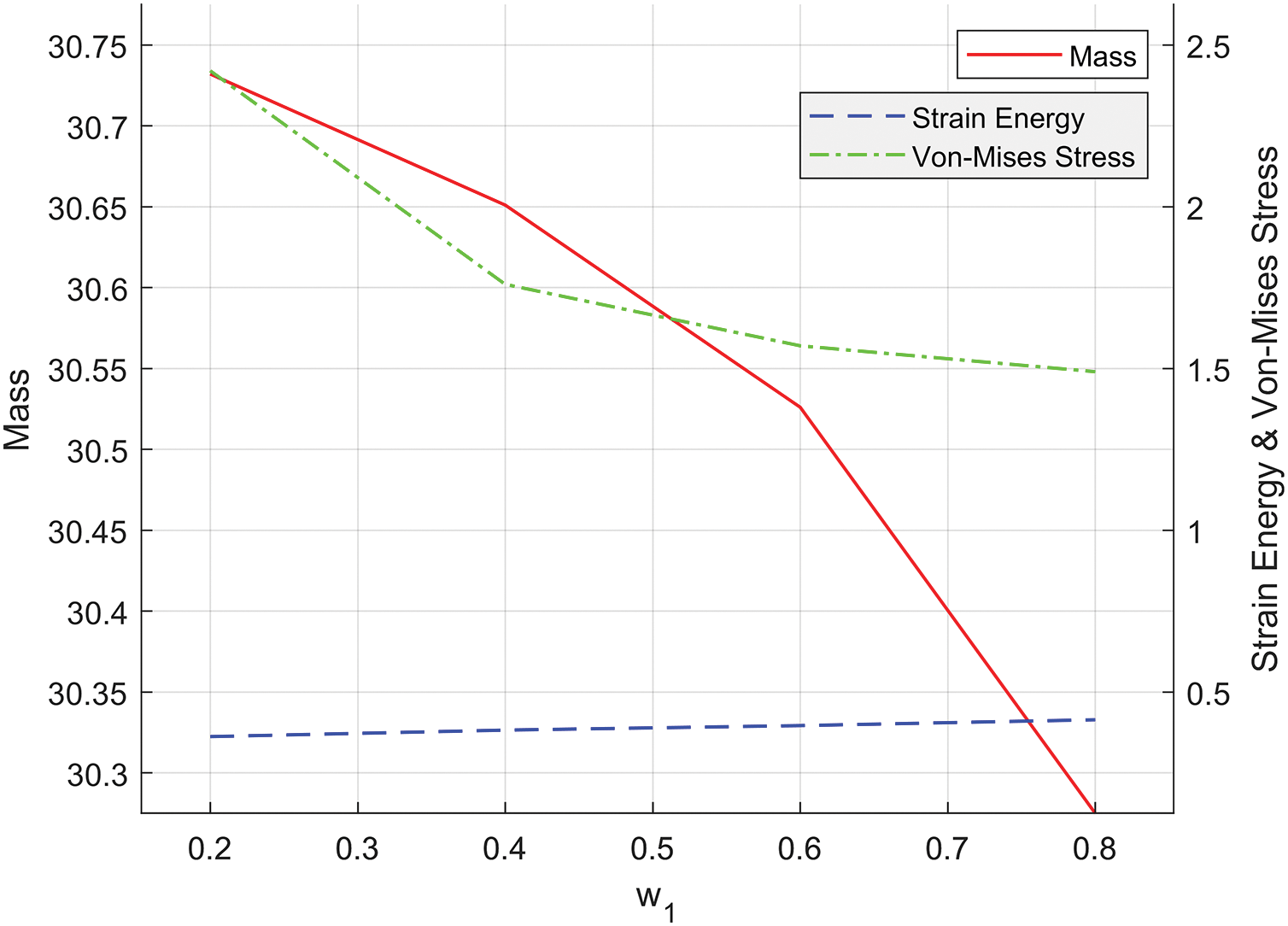
Figure 4: Effect of varying weight coefficients w1 on strain energy and Von-Mises stress for MBB beam

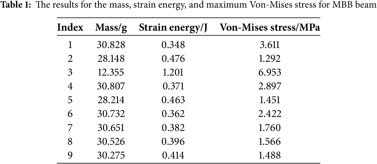
As shown in Table 1, it is evident that, using the method described in this study for the coordinated topology optimization of stiffness and strength in the MBB beam, the optimized structures under different weight coefficients exhibit similar mass to the model Q1. The maximum strain energy is only slightly higher than that of the model Q1, with a maximum difference of 0.066 J. The maximum Von-Mises stress falls between the values of model Q1 and model Q2, with a minimum difference of 0.2 MPa and a maximum difference of 2.12 MPa. Furthermore, compared with model Q4, the method proposed in this paper can not only reduce the strain energy but also maintain the maximum stress to be basically consistent with that of model Q4 (as can be seen from the comparison in rows 4 and 6 in the table). Compared with Model Q5, this method can significantly reduce the maximum stress value and strain energy (as can be seen from the comparison in rows 5 and 9 in the table).

To further highlight the computational advantages of the methods presented in this paper, the calculation times for the MBB beam case of each optimization model were statistically analyzed, as shown in Table 2.

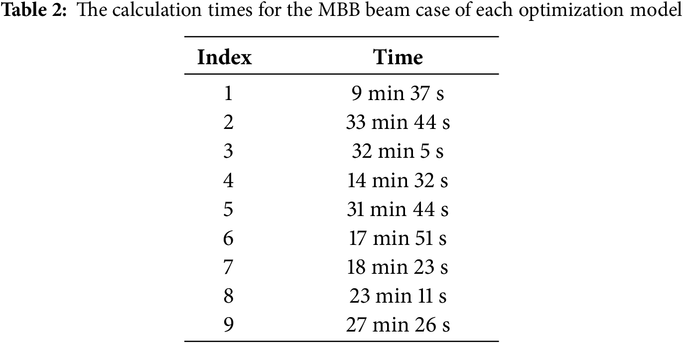
From Table 2, it can be seen that the calculation time is the shortest only when optimizing the topology of model Q1. When stress constraints are added, regardless of whether they are used as the objective function or constraints, the calculation time will increase compared to the topology optimization design of model Q1. However, the longest calculation time is for model Q2 topology optimization. The calculation times of other models are between those of model Q1 and model Q2 topology optimization. In this method, as the weight coefficient w increases, the weight assigned to global stress aggregation also increases. The calculation time increases slightly, but the increase is not significant. And under all weight coefficients, the calculation time is less than the stress minimization topology optimization and is between model Q4 and model Q5. When w=0.2, the calculation time of this method increases by approximately 3 min compared to model Q4. When w=0.8, the calculation time of this method decreases by approximately 4 min compared to model Q5. This is because the calculation of strain energy is linear, while the calculation of stress is non-linear. When the weight coefficient for stress allocation is large, the non-linear calculation weight increases, and the calculation time will increase. In any case, it is the same.

In conclusion, the proposed method effectively ensures both stiffness (maximized strain energy) and significantly reduces stress (enhancing strength and durability), thereby achieving a coordinated topology optimization design for stiffness and strength in the MBB beam.

4.2 L-Shaped Bracket

To address the issue in the MBB case where the stress constraint under pure pressure loading was ineffective, two loading conditions are used for the numerical calculations in this case. The maximum stress in the L-shaped bracket occurs at the corner under the action of force F1. Therefore, the subsequent topology optimization results for the L-shaped structure are extracted under this loading condition.

The second numerical case involves the well-known L-shaped bracket. The dimensions and boundary conditions are shown in Fig. 5. The thickness is 1.0 mm. The design domain is discretized into 108,816 three-node plane stress elements, with a unit length of 1.0 mm and a filter radius rmin of 3.0 mm. A fixed boundary condition is applied to the upper edge. To avoid stress concentration, a vertical force F1,2 = 4 N is applied to a 10 mm section on the upper-right side of the L-shaped bracket. The specified volume fraction is 0.4. The maximum stress occurs at the right-angle corner, with a value of 3.03 MPa.

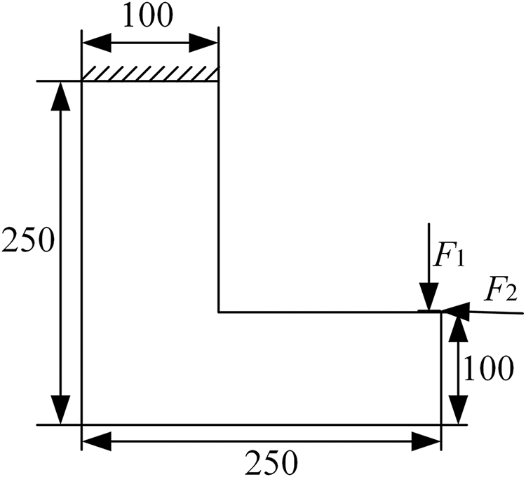
Figure 5: The dimensional schematic and boundary conditions of the L-shaped bracket

Fig. 6 presents the topology optimization results for the L-bracket design using six different optimization models in this study. Specifically, Fig. 6a illustrates the topology optimized for compliance minimization under the Q1 model. Fig. 6b shows the topology optimized for stress minimization under the Q2 model. Fig. 6c presents the topology optimized for mass minimization with both stress and compliance constraints, following the Q5 model. Fig. 6d represents the topology optimized for compliance minimization with stress constraints, as per the Q3 model. Fig. 6e displays the topology optimized for stress minimization with compliance constraints, based on the Q4 model. Fig. 6f–i presents the structural stiffness-stress coordinated design results for the Q6 model, with weight coefficients w1 = 0.2, 0.4, 0.6, and 0.8.

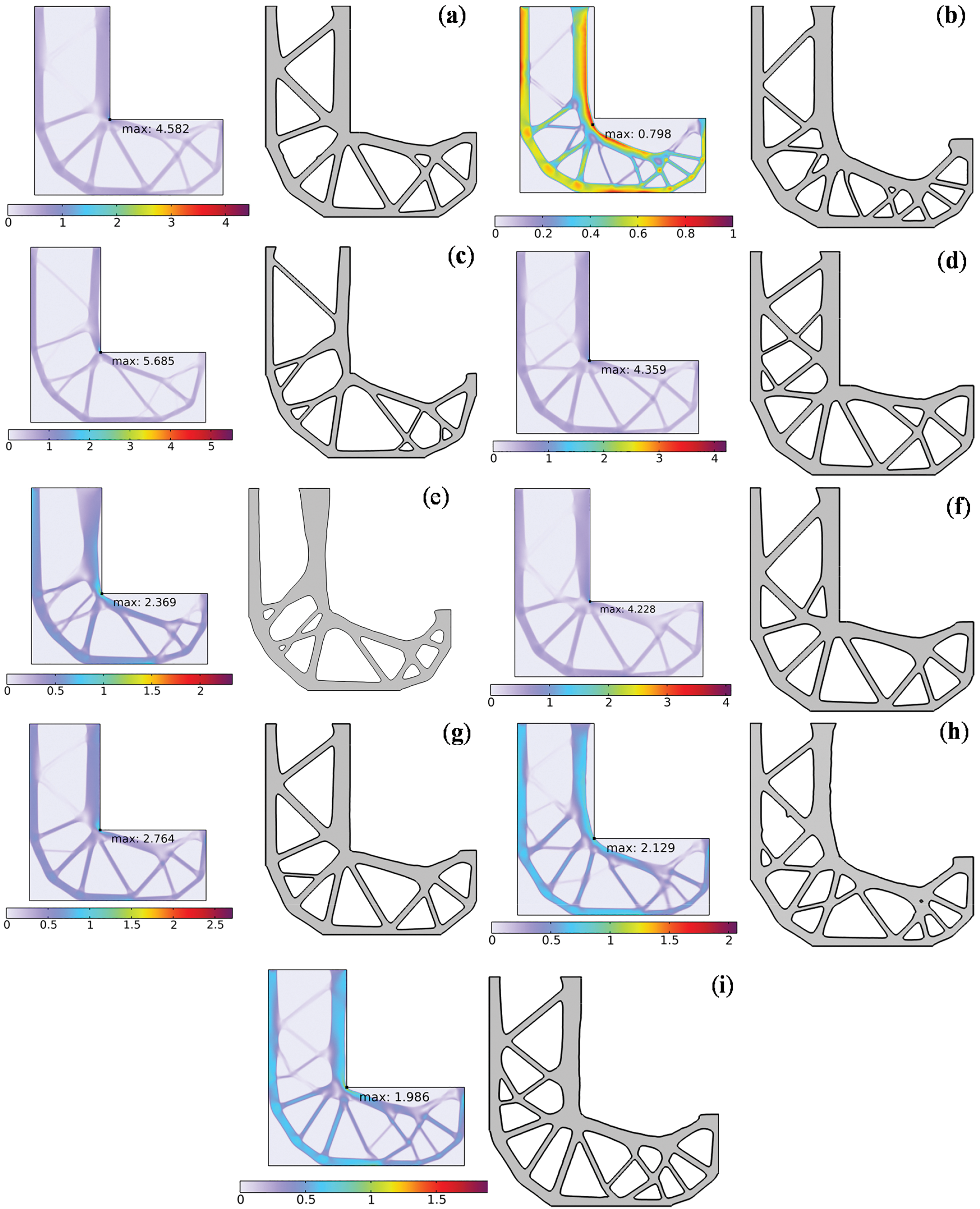
Figure 6: The result of the L-shaped bracket. (a) Q1; (b) Q2; (c) Q3; (d) Q4; (e) Q5; (f) Q6 when w1 = 0.2; (g) Q6 when w1 = 0.4; (h) Q6 when w1 = 0.6; (i) Q6 when w1 = 0.8

Fig. 6a,b presents similar topology structures. However, the stress at the right-angle corner in Fig. 6a is significantly higher than in Fig. 6b, by approximately a factor of six. This demonstrates the pronounced effect of using an aggregate function for structural stress minimization.

In Fig. 6c, the topology structure after optimization of flexibility and stress constraints is different from that in Fig. 6a. Although the strain energy remains almost unchanged, the mass has decreased by nearly 42 g, and the stress at the right-angle corners has increased by 1.1 MPa. Compared with Fig. 6b, the maximum stress at the right-angle corners in Fig. 6c is 8 times that of it, although Fig. 6c can obtain a lighter topology structure, the maximum stress value in the structure cannot be guaranteed.

The topological structure in Fig. 6d incorporates stress constraints, which is different from the structure in Fig. 6a. After adding the stress constraints, the quality strain energy and the maximum stress slightly decreased, but the change was very small. This indicates that the stress constraints have an effect, but the effect is not significant.

The topological structure in Fig. 6e represents the minimized stress result with flexibility constraints included. This is different from the structure in Fig. 6a. The mass slightly decreases, but the change is very small. The strain energy slightly increases, but the change is also not significant. However, the maximum stress has decreased by 2.2 MPa. This indicates that the stress constraint has a significant effect on the objective function’s reduction of the maximum stress value.

Fig. 6f–i shows the topology structures with varying weight coefficients w1. As w1 increases, the mass remains nearly constant, while strain energy increases gradually with a small variation. The maximum stress at the right-angle corner decreases steadily, with the most significant reduction occurring when w1 is set to 0.2 and 0.4, achieving a roughly 50% reduction. To further clarify the capability of the proposed method in coordinating stiffness and strength, the changes in strain energy and the maximum Von Mises stress within the structure for different weight coefficients are plotted in Fig. 7. The results for mass, strain energy, and the maximum Von Mises stress at the right-angle corner for each optimization model are presented in Table 2.

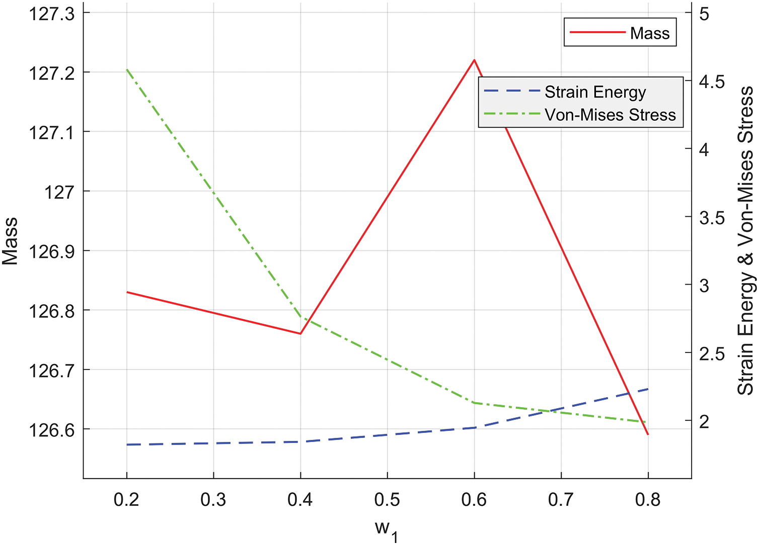
Figure 7: Effect of varying weight coefficients w1 on strain energy and Von-Mises stress for L-shaped bracket

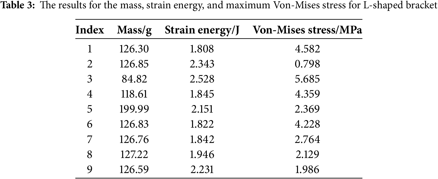
As shown in Table 3, it is evident that, when the L-bracket is optimized using the method presented in this study, the mass of the optimized structure remains nearly the same across different weight values, consistent with the model Q1. The maximum strain energy is only marginally higher than the value obtained from model Q1, with a maximum difference of 0.42 J. The maximum Von Mises stress falls between the values achieved from model Q1 and model Q2, with a minimum difference of 0.3 MPa and a maximum difference of 2.59 MPa. Furthermore, since this study only focuses on the coordinated design of model stiffness and stress, the comparison regarding mass can be disregarded. Only the comparison based on strain energy and maximum stress is conducted. Compared with Model Q4, the method proposed in this paper not only can reduce the maximum stress value by 1.595 MPa but also can make the strain energy basically the same as Model Q4 (as can be seen from the comparison in the 4th and 7th rows of the table). Compared with Model Q5, both the strain energy and the maximum stress have decreased, to 0.2 J and 0.2 MPa, respectively (as can be seen from the comparison in the 5th and 8th rows of the table).

To further highlight the computational advantages of the methods presented in this paper, the calculation times for the L-shaped bracket case of each optimization model were statistically analyzed, as shown in Table 4.

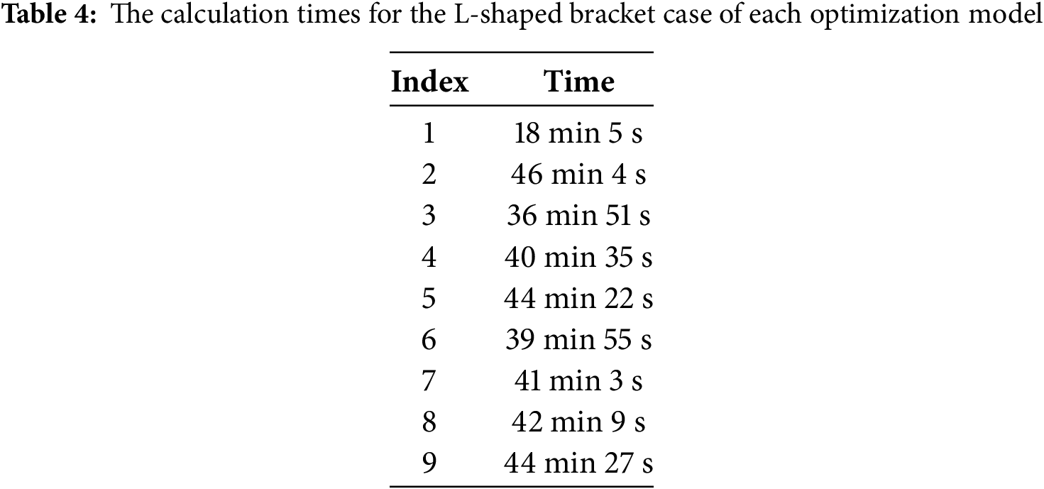
From Table 4, the calculation time is the shortest only when optimizing the topology of model Q1. When stress constraints are added, regardless of whether they are used as the objective function or constraints, the calculation time will increase compared to the topology optimization design of model Q1. However, the longest calculation time is that of model Q2 topology optimization. The calculation times of other models are between those of model Q1 and model Q2 topology optimization. As the weight coefficient w increases in this method, the weight assigned to global stress aggregation also increases, resulting in a certain increase in calculation time, but the increase is not significant. And under all weight coefficients, the calculation time is less than that of stress minimization topology optimization and is between model Q4 and model Q5. When w=0.2, the calculation time of this method is reduced by approximately 1 min compared to model Q4. When w=0.8, the calculation time of this method is basically the same as that of model Q5. This is because the calculation of strain energy is linear, while the calculation of stress is non-linear. When the weight coefficient for stress allocation is large, the non-linear calculation weight increases, and the calculation time will increase. In any case, the same applies. Of course, the total calculation time is also related to the model’s geometric shape and loading conditions. But in general, this method also has a calculation time that is basically comparable to model Q4 and model Q5.

In conclusion, the proposed method ensures both structural stiffness (maximum strain energy) and a significant reduction in stress (enhancing strength and durability), thereby achieving a balanced topological design that coordinates stiffness and strength for the L-shape bracket.

4.3 3D Bracket

To fully verify the effectiveness and applicability of the method proposed in this paper, the method was applied to a three-dimensional solid structure. The structural dimensions are shown in Fig. 8 below.

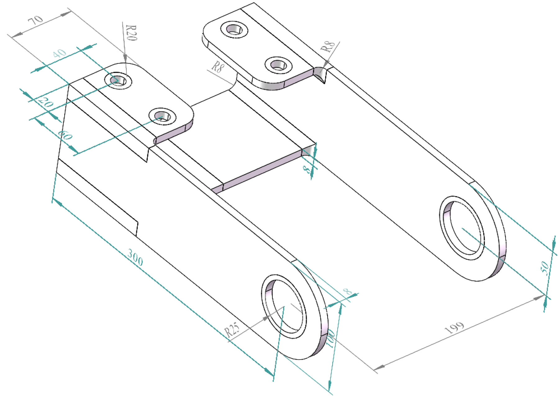
Figure 8: The dimensional schematic of the 3D bracket

The design area is divided into 220,248 units, with each unit having a length of 2.5 mm and a filtering radius rmin of 5.0 mm. The four small circular holes at the top adopt fixed boundary conditions. On the surfaces of the two large circular holes, an axial load with a peak of 2.5 MPa is applied, and the specified volume fraction is 0.5. The maximum stress occurs at the edge of the middle small circular hole, with a value of 117.729 MPa.

Fig. 9 presents the topological optimization results of the 3D bracket using six different optimization models in this study. Specifically, Fig. 9a shows the topological optimization results for minimizing stiffness under the Q1 model. Fig. 9b shows the topological optimization results for minimizing stress under the Q2 model. Fig. 9c demonstrates the topological optimization results following the Q3 model for minimizing mass while considering both stress and stiffness constraints. Fig. 9d represents the topological optimization results for minimizing stiffness while considering stress constraints under the Q4 model. Fig. 9e shows the topological optimization results based on the Q5 model for minimizing stress while considering stiffness constraints. Fig. 9f–i presents the structural stiffness-stress coordination design results for the Q6 model, with weight coefficients of 0.2, 0.4, 0.6, and 0.8, respectively.

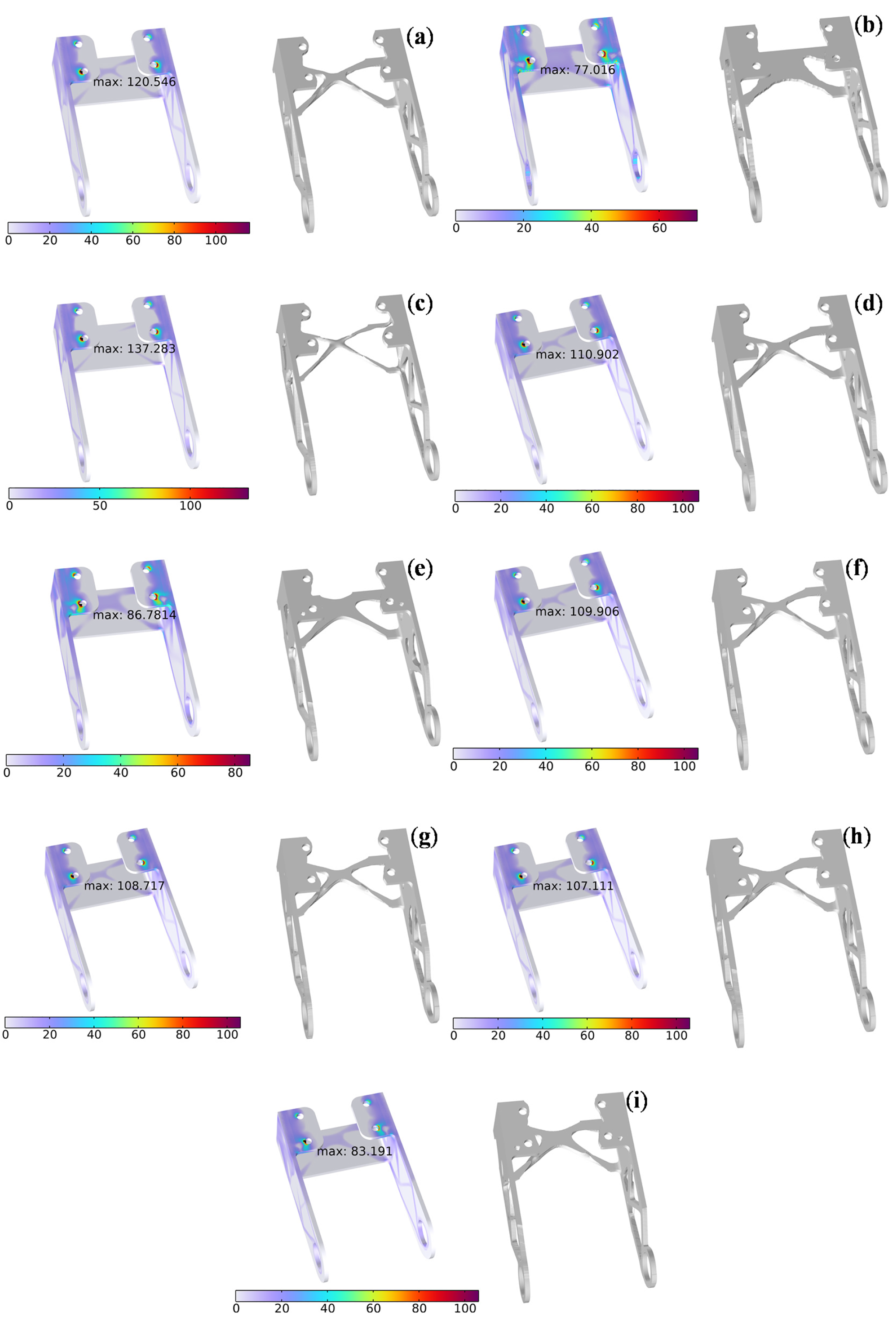
Figure 9: The result of 3D bracket. (a) Q1; (b) Q2; (c) Q3; (d) Q4; (e) Q5; (f) Q6 when w1 = 0.2; (g) Q6 when w1 = 0.4; (h) Q6 when w1 = 0.6; (i) Q6 when w1 = 0.8

Fig. 9a,b exhibits similar topological structures in terms of mass and strain energy. However, the stress on the side of the small cylinder on the left in Fig. 9a is significantly higher than that in Fig. 9b, approximately 1.5 times higher. This indicates that the effect of using the aggregation function to minimize the structural stress is very significant.

In Fig. 9c, the topology structure after stress constraint optimization is basically the same as that in Fig. 9a. The mass has been significantly reduced by approximately 1 kg, the strain energy remains basically unchanged, but the maximum stress value has increased significantly to 16.737 MPa.

The topological structure in Fig. 9d is not much different from that in Fig. 9a. However, the stress difference is nearly 10 MPa, which also indicates that under the influence of stress constraints, the maximum stress value in the model can be effectively reduced.

In Fig. 9e, its topological structure is different from that in Fig. 9b. It can be observed that after applying the compliance constraint, The maximum stress value has increased by 9.765 MPa.

Fig. 9f–i shows that as the weight coefficient increases, the quality and strain energy remain almost unchanged, while the maximum stress value shows a relatively small variation in the early stage. However, from 0.6 to 0.8, the maximum stress value decreases significantly. To more clearly demonstrate the coordination relationship between stiffness and strength in the proposed method, Fig. 10 presents the variation curves of strain energy and the maximum von-mises stress under different weight coefficients. The optimized results of the quality, strain energy, and maximum Von-Mises stress of all models are summarized in Table 5.

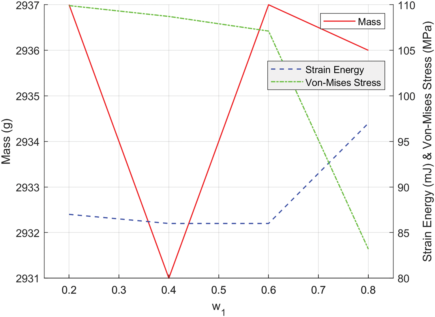
Figure 10: Effect of varying weight coefficients w1 on strain energy and Von-Mises stress for 3D bracket

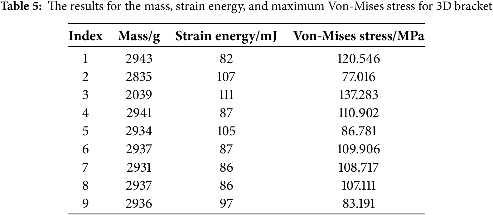
As shown in Table 5, it is evident that when the optimization method proposed in this study is applied to optimize the 3D scaffold, the quality of the optimized structure remains almost unchanged under different weight values, which is consistent with Model Q1. The maximum strain energy is only slightly higher than the value obtained by Model Q1, with a maximum difference of 15 mJ. The maximum Von-Mises stress is between the values achieved by Model Q1 and Model Q2, with a minimum difference of 10 MPa and a maximum difference of 37 MPa. Moreover, since this study only focuses on the collaborative design of model stiffness and stress, the comparison in terms of quality can be ignored. Only comparisons based on strain energy and maximum stress are conducted. Compared with Model Q4, the method proposed in this paper not only can reduce the maximum stress value by 27.711 MPa but also can make the strain energy approximately the same as Model Q4. Compared with Model Q5, its strain energy has decreased by 18 mJ, and the maximum stress value is approximately decreased by about 3.5 MPa compared to Model Q5 (as can be seen from the comparison in the 5th and 8th rows of the table).

To further highlight the computational advantages of the methods presented in this paper, the calculation times for the L-shaped bracket case of each optimization model were statistically analyzed, as shown in Table 6.

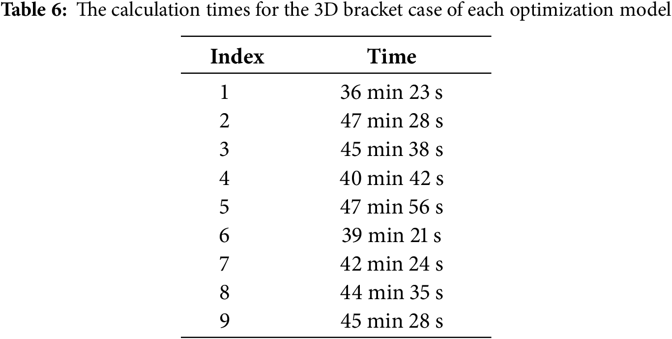
From Table 6, when the topological structure of model Q1 is optimized, the calculation time is the shortest. When stress constraints are added, regardless of whether these constraints are used as the objective function or constraints, compared with the topological optimization design of model Q1, the calculation time will increase. However, the longest calculation time is that of the topological optimization calculation of model Q2. The calculation time of other models is between the topological optimization calculation time of model Q1 and model Q2. In this method, as the weight coefficient w increases, the weight assigned to global stress aggregation also increases, resulting in a certain increase in calculation time, but the increase is not significant. Moreover, under all weight coefficients, the calculation time of this method is less than that of stress minimization topological optimization and is between that of model Q4 and model Q5. When w=0.2, compared with model Q4, the calculation time of this method is approximately reduced by 1 min. When w=0.8, the calculation time of this method is reduced by about 2 min compared to model Q5. This is because the calculation of strain energy is linear, while the calculation of stress is non-linear. When the weight coefficient of stress allocation is large, the weight of non-linear calculation will also increase, and the calculation time will also be prolonged. No matter what the case is, it is the same. Of course, the total calculation time is also related to the geometric shape and loading conditions of the model. But overall, the calculation time of this method is close to that of model Q4 and model Q5 compared to model Q4 and model Q5.

In conclusion, the proposed method ensures both structural stiffness (maximum strain energy) and a significant reduction in stress (enhancing strength and durability), thereby achieving a balanced topological design that coordinates stiffness and strength for the 3D bracket.

It is worth noting that the method proposed in this paper aims to verify the correctness of the approach. There is relatively less discussion on the issues of fine branches and manufacturability in the above three numerical cases. The minimum length scale rmin in Eq. (30) can be incorporated as a core parameter into the optimization model: by adjusting the value of rmin , the aforementioned problems can be effectively addressed.

4.4 Performance Evaluation Analysis

In multi-objective optimization, it is essential to identify the optimal trade-off between the objective functions. Based on the numerical results of the three cases above, the weight values for the two objective functions [46] are determined according to Eq. (32).

z=‖∑i[f1∗−fi(x)fi(x)]‖(32)

where fi∗ represents the ideal feasible solution for each single objective, and fi(x) represents a set of Pareto solutions obtained from multi-objective optimization. When z is minimized, fi(x) corresponds to the optimal compromise solution. Clearly, the optimal topological values for strain energy, Von Mises stress, and mass have been obtained from the single-objective optimizations in examples Q1, Q2, and Q5, which are considered as the ideal feasible solutions for the single objectives.

To determine the weight coefficient w1 that yields the optimal compromise solution in multi-objective optimization, the objective values from Q1 and Q2, as well as the multi-objective value from Q6, are substituted into Eq. (32). The corresponding decision function value for each weight w1 is calculated, and the Pareto solution corresponding to the minimum decision function value is selected as the optimal compromise solution. The results are shown in Tables 7–9.

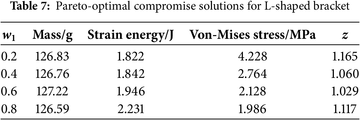
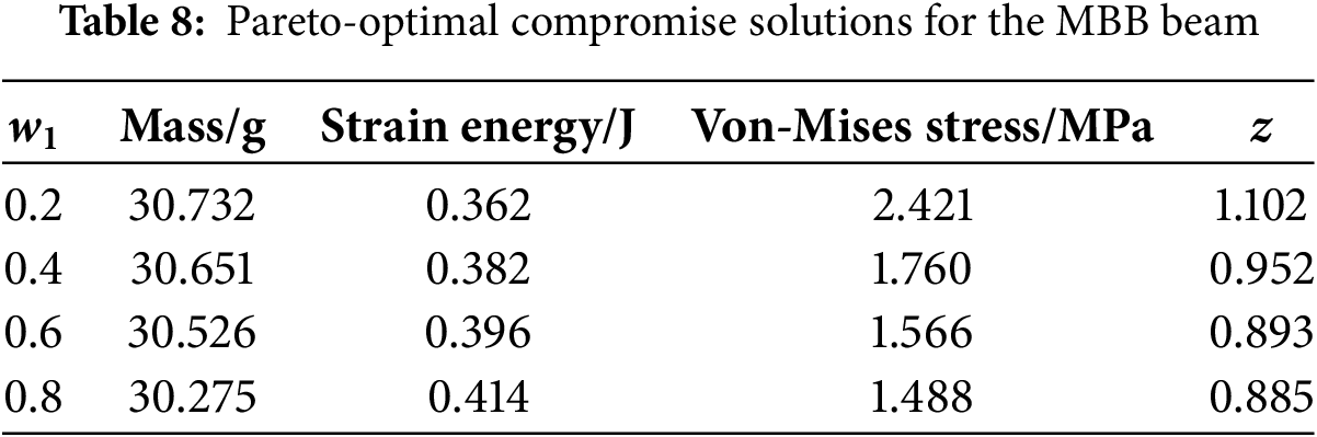
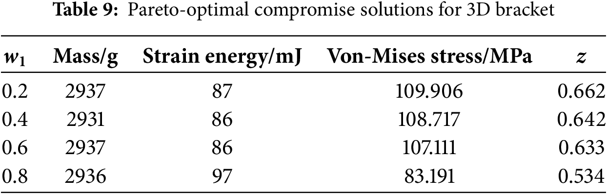
From Tables 7–9, it is evident that in the case of L-bracket, when w1 = 0.6, the decision function reaches its minimum value of 1.029. Therefore, the Pareto solution at this point is selected as the optimal compromise, with a mass of 127.22 g, strain energy of 1.946 J, and maximum Von Mises stress of 2.128 MPa. In the MBB beam case, when w1 = 0.8, the decision function reaches its minimum value of 0.885. The corresponding Pareto solution is selected as the optimal compromise, with a mass of 30.275 g, strain energy of 0.414 J, and maximum Von Mises stress of 1.49 MPa. In the 3D bracket case, when w1 = 0.8, the decision function reaches its minimum value of 0.534. The corresponding Pareto solution is selected as the optimal compromise, with a mass of 2936 g, strain energy of 97 mJ, and maximum Von Mises stress of 83.191 MPa.

The above describes the selection of the weight coefficient w1 by considering three factors: quality, strain energy, and maximum stress. If the weight coefficient w1 value is directly determined based on the two factors of strain energy and global stress measurement, the Pareto solution will change. The following will provide a detailed explanation.

In Eq. (31), fi∗ should be the strain energy in Model Q1 and the global stress measurement value in Model Q2. The global stress measurements of the three models are 0.231, 0.613, and 0.313, respectively. fi(x) represents a set of Pareto solutions obtained from multi-objective optimization.

To determine the weight coefficient w1 that yields the optimal compromise solution in multi-objective optimization, the objective values from Q1 and Q2, as well as the multi-objective value from Q6, are substituted into Eq. (31). The corresponding decision function value for each weight w1 is calculated, and the Pareto solution corresponding to the minimum decision function value is selected as the optimal compromise solution. The results are shown in Tables 10–12.

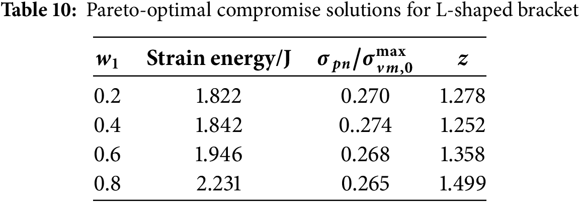
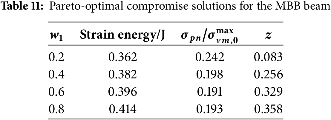
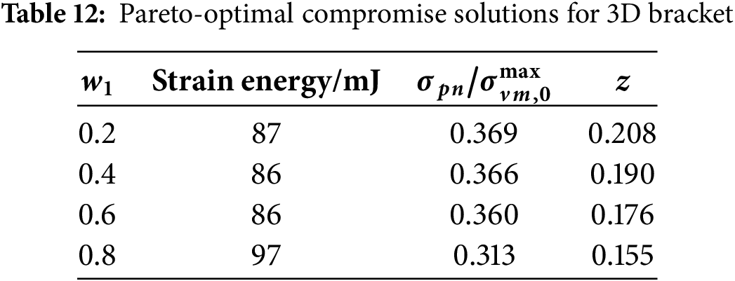
From Tables 10–12, it is evident that in the case of L-bracket, when w1 = 0.4, the decision function reaches its minimum value of 1.252. Therefore, the Pareto solution at this point is selected as the optimal compromise, with a mass of 126.76 g, strain energy of 1.842 J, and maximum Von Mises stress of 2.764 MPa. In the MBB beam case, when w1 = 0.2, the decision function reaches its minimum value of 0.083. The corresponding Pareto solution is selected as the optimal compromise, with a mass of 30.732 g, strain energy of 0.362 J, and maximum Von Mises stress of 2.421 MPa. In the 3D bracket case, when w1 = 0.8, the decision function reaches its minimum value of 0.155. The corresponding Pareto solution is selected as the optimal compromise, with a mass of 2936 g, strain energy of 97 mJ, and maximum Von Mises stress of 83.191 MPa.

From the above, when determining the multi-objective weight coefficients, considering the influence of different factors, the Pareto solution will change, and thus the selection of weight coefficients will also change. Therefore, the specific weight coefficients should be determined according to the actual situation.

5  Conclusion

This study proposed a stiffness-strength collaborative topology optimization method based on an objective normalization strategy. By formulating a dual-objective mixed sensitivity analysis, the method overcomes the limitations of traditional single-objective topology optimization. The introduction of a regularized weighting factor enables a well-balanced design by simultaneously enhancing stiffness to reduce deformation and ensure sufficient strength to prevent failure.

To validate the effectiveness of the proposed approach, numerical experiments were conducted on the MBB beam, L-shaped bracket, and the 3D bracket cases, The results demonstrated significant improvements in structural performance:

(1)   For the MBB beam, the peak strain energy increased by 24% (compared to single-objective strength optimization), while the peak stress was reduced by 59% (compared to single-objective stiffness optimization). The optimal trade-off solution was achieved at a specific weight ratio, yielding a performance index z = 0.885.

(2)   For the L-shaped bracket, the peak strain energy increased by 22%, and the peak stress decreased by 57% under the same comparative conditions. The best compromise solution was obtained at a corresponding weight ratio, with a performance index z = 1.029.

(3)   For the 3D bracket, the peak strain energy increased by 20%, and the peak stress decreased by 31% under the same comparative conditions. The best compromise solution was obtained at a corresponding weight ratio, with a performance index z = 0.534.

In summary, the proposed method offers a systematic and computationally efficient approach for achieving well-balanced stiffness-strength topology optimization. Future work will focus on extending the framework to multi-material structures and incorporating adaptive weight strategies to further enhance its applicability in complex engineering scenarios.

Acknowledgement: Not applicable.

Funding Statement: This study is funded by National Nature Science Foundation of China (92266203), National Nature Science Foundation of China (52205278), Key Projects of Shijiazhuang Basic Research Program (241791077A), Central Guide Local Science and Technology Development Fund Project of Hebei Province (246Z1022G).

Author Contributions: The authors confirm contribution to the paper as follows: Writing—original draft, Jianchang Hou; Methodology, Jianchang Hou, Zhanpeng Jiang and Weicheng Li; Writing—review & editing, Zhanpeng Jiang; Validation, Hui Lian, Zhaohua Wang and Zijian Liu; Visualization, Hui Lian; Formal analysis, Zijian Liu; Resources, Fenghe Wu; Funding acquisition, Fenghe Wu and Zhaohua Wang. All authors reviewed the results and approved the final version of the manuscript.

Availability of Data and Materials: The data that support the findings of this study are available from the Corresponding Author, Weicheng Li, upon reasonable request.

Ethics Approval: Not applicable.

Conflicts of Interest: The authors declare no conflicts of interest to report regarding the present study.

References

1. Bendsøe MP, Kikuchi N. Generating optimal topologies in structural design using a homogenization method. Comput Methods Appl Mech Eng. 1988;71(2):197–224. doi:10.1016/0045-7825(88)90086-2. [Google Scholar] [CrossRef]

2. Jankowski R, Manguri A, Hassan H, Saeed N. Topology, size, and shape optimization in civil engineering structures: a review. Comput Model Eng Sci. 2025;142(2):933–71. doi:10.32604/cmes.2025.059249. [Google Scholar] [CrossRef]

3. Banh TT, Lee D. Efficient topology optimization for geometrically nonlinear multi-material systems under design-dependent pressure loading. Eng Comput. 2025;41(2):1155–89. doi:10.1007/s00366-024-02083-y. [Google Scholar] [CrossRef]

4. Bendsøe MP. Optimal shape design as a material distribution problem. Struct Optim. 1989;1(4):193–202. doi:10.1007/BF01650949. [Google Scholar] [CrossRef]

5. Rozvany G. Aims, scope, methods, history and unified terminology of computer-aided topology optimization in structural mechanics. Struct Multidisc Optim. 2001;21(2):90–108. doi:10.1007/s001580050174. [Google Scholar] [CrossRef]

6. Luo Z, Zhang N, Wu T. Design of compliant mechanisms using meshless level set methods. Comput Model Eng Sci. 1970;85:299–328. doi:10.3970/cmes.2012.085.299. [Google Scholar] [CrossRef]

7. Wang MY, Wang X, Guo D. A level set method for structural topology optimization. Comput Methods Appl Mech Eng. 2003;192(1-2):227–46. doi:10.1016/S0045-7825(02)00559-5. [Google Scholar] [CrossRef]

8. Allaire G. Structural optimization using sensitivity analysis and a level-set method. J Comput Phys. 2004;194(1):363–93. doi:10.1016/j.jcp.2003.09.032. [Google Scholar] [CrossRef]

9. Zong H, Liu H, Ma Q, Tian Y, Zhou M, Wang MY. VCUT level set method for topology optimization of functionally graded cellular structures. Comput Methods Appl Mech Eng. 2019;354(1838):487–505. doi:10.1016/j.cma.2019.05.029. [Google Scholar] [CrossRef]

10. Xie YM, Steven GP. A simple evolutionary procedure for structural optimization. Comput Struct. 1993;49(5):885–96. doi:10.1016/0045-7949(93)90035-C. [Google Scholar] [CrossRef]

11. Xie YM, Steven GP. Optimal design of multiple load case structures using an evolutionary procedure. Eng Comput. 1994;11(4):295–302. doi:10.1108/02644409410799290. [Google Scholar] [CrossRef]

12. Xie YM, Steven GP. Evolutionary structural optimization for dynamic problems. Comput Struct. 1996;58(6):1067–73. doi:10.1016/0045-7949(95)00235-9. [Google Scholar] [CrossRef]

13. Qian X. Topology optimization in B-spline space. Comput Methods Appl Mech Eng. 2013;265(2):15–35. doi:10.1016/j.cma.2013.06.001. [Google Scholar] [CrossRef]

14. Lin D, Gao L, Gao J. The Lagrangian-Eulerian described particle flow topology optimization (PFTO) approach with isogeometric material point method. Comput Methods Appl Mech Eng. 2025;440:117892. doi:10.1016/j.cma.2025.117892. [Google Scholar] [CrossRef]

15. Gao J, Chen C, Fang X. Multi-objective topology optimization for solid-porous infill designs in regions-divided structures using multi-patch isogeometric analysis. Comput Methods Appl Mech Eng. 2024;428:117095. doi:10.1016/j.cma.2024.117095. [Google Scholar] [CrossRef]

16. Guo X, Zhang W, Zhang J, Yuan J. Explicit structural topology optimization based on moving morphable components (MMC) with curved skeletons. Comput Methods Appl Mech Eng. 2016;310:711–48. doi:10.1016/j.cma.2016.07.018. [Google Scholar] [CrossRef]

17. Zhang W, Li D, Zhang J, Guo X. Minimum length scale control in structural topology optimization based on the Moving Morphable Components (MMC) approach. Comput Methods Appl Mech Eng. 2016;311:327–55. doi:10.1016/j.cma.2016.08.022. [Google Scholar] [CrossRef]

18. Hoang VN, Nguyen NL, Nguyen-Xuan H. Topology optimization of coated structure using moving morphable sandwich bars. Struct Multidiscip Optim. 2020;61(2):491–506. doi:10.1007/s00158-019-02370-z. [Google Scholar] [CrossRef]

19. Wu J, Clausen A, Sigmund O. Minimum compliance topology optimization of shell-infill composites for additive manufacturing. Comput Methods Appl Mech Eng. 2017;326(2):358–75. doi:10.1016/j.cma.2017.08.018. [Google Scholar] [CrossRef]

20. Guo L, Meng Z, Wang X. A new concurrent optimization method of structural topologies and continuous fiber orientations for minimum structural compliance under stress constraints. Adv Eng Softw. 2024;195(2):103688. doi:10.1016/j.advengsoft.2024.103688. [Google Scholar] [CrossRef]

21. Yu C, Wang Q, Mei C, Xia Z. Multiscale isogeometric topology optimization with unified structural skeleton. Comput Model Eng Sci. 2020;122(3):779–803. doi:10.32604/cmes.2020.09363. [Google Scholar] [CrossRef]

22. Nabaki K, Shen J, Huang X. Stress minimization of structures based on bidirectional evolutionary procedure. J Struct Eng. 2019;145(2):04018256. doi:10.1061/(ASCE)ST.1943-541X.0002264. [Google Scholar] [CrossRef]

23. Nabaki K, Shen J, Huang X. Evolutionary topology optimization of continuum structures considering fatigue failure. Mater Des. 2019;166(5):107586. doi:10.1016/j.matdes.2019.107586. [Google Scholar] [CrossRef]

24. Zhang W, Li D, Zhou J, Du Z, Li B, Guo X. A moving morphable void (MMV)-based explicit approach for topology optimization considering stress constraints. Comput Methods Appl Mech Eng. 2018;334:381–413. doi:10.1016/j.cma.2018.01.050. [Google Scholar] [CrossRef]

25. Le C, Norato J, Bruns T, Ha C, Tortorelli D. Stress-based topology optimization for continua. Struct Multidisc Optim. 2010;41(4):605–20. doi:10.1007/s00158-009-0440-y. [Google Scholar] [CrossRef]

26. Moter A, Abdelhamid M, Czekanski A. Direction-oriented stress-constrained topology optimization of orthotropic materials. Struct Multidisc Optim. 2022;65(6):177. doi:10.1007/s00158-022-03269-y. [Google Scholar] [CrossRef]

27. Kundu RD, Zhang XS. Stress-based topology optimization for fiber composites with improved stiffness and strength: integrating anisotropic and isotropic materials. Compos Struct. 2023;320(1):117041. doi:10.1016/j.compstruct.2023.117041. [Google Scholar] [CrossRef]

28. Nguyen MN, Lee D. Design of the multiphase material structures with mass, stiffness, stress, and dynamic criteria via a modified ordered SIMP topology optimization. Adv Eng Softw. 2024;189(4):103592. doi:10.1016/j.advengsoft.2023.103592. [Google Scholar] [CrossRef]

29. Yang RJ, Chen CJ. Stress-based topology optimization. Struct Optim. 1996;12(2–3):98–105. doi:10.1007/BF01196941. [Google Scholar] [CrossRef]

30. Duysinx P, Sigmund O. New developments in handling stress constraints in optimal material distribution. In: 7th AIAA/USAF/NASA/ISSMO Symposium on Multidisciplinary Analysis and Optimization; 1998 Sep 2–4; Louis, MO, USA. doi:10.2514/6.1998-4906. [Google Scholar] [CrossRef]

31. Zhang WS, Guo X, Wang MY, Wei P. Optimal topology design of continuum structures with stress concentration alleviation via level set method. Int J Numer Methods Eng. 2013;93(9):942–59. doi:10.1002/nme.4416. [Google Scholar] [CrossRef]

32. París J, Navarrina F, Colominas I, Casteleiro M. Block aggregation of stress constraints in topology optimization of structures. Adv Eng Softw. 2010;41(3):433–41. doi:10.1016/j.advengsoft.2009.03.006. [Google Scholar] [CrossRef]

33. Cheng GD, Guo X. ε-relaxed approach in structural topology optimization. Struct Optim. 1997;13(4):258–66. doi:10.1007/BF01197454. [Google Scholar] [CrossRef]

34. Bruggi M. On an alternative approach to stress constraints relaxation in topology optimization. Struct Multidisc Optim. 2008;36(2):125–41. doi:10.1007/s00158-007-0203-6. [Google Scholar] [CrossRef]

35. Bruggi M, Duysinx P. Topology optimization for minimum weight with compliance and stress constraints. Struct Multidisc Optim. 2012;46(3):369–84. doi:10.1007/s00158-012-0759-7. [Google Scholar] [CrossRef]

36. Fan Z, Xia L, Lai W, Xia Q, Shi T. Evolutionary topology optimization of continuum structures with stress constraints. Struct Multidisc Optim. 2019;59(2):647–58. doi:10.1007/s00158-018-2090-4. [Google Scholar] [CrossRef]

37. Ferro N, Micheletti S, Perotto S. Compliance-stress constrained mass minimization for topology optimization on anisotropic meshes. SN Appl Sci. 2020;2(7):1196. doi:10.1007/s42452-020-2947-1. [Google Scholar] [CrossRef]

38. Ma C, Gao Y, Duan Y, Liu Z. Stress relaxation and sensitivity weight for bi-directional evolutionary structural optimization to improve the computational efficiency and stabilization on stress-based topology optimization. Comput Model Eng Sci. 2021;126(2):715–38. doi:10.32604/cmes.2021.011187. [Google Scholar] [CrossRef]

39. Zhai X, Chen F, Wu J. Alternating optimization of design and stress for stress-constrained topology optimization. Struct Multidisc Optim. 2021;64(4):2323–42. doi:10.1007/s00158-021-02985-1. [Google Scholar] [CrossRef]

40. Liu J, Yan J, Yu H. Stress-constrained topology optimization for material extrusion polymer additive manufacturing. J Comput Des Eng. 2021;8(3):979–93. doi:10.1093/jcde/qwab028. [Google Scholar] [CrossRef]

41. Zheng J, Zhang G, Jiang C. Stress-based topology optimization of thermoelastic structures considering self-support constraints. Comput Methods Appl Mech Eng. 2023;408(1):115957. doi:10.1016/j.cma.2023.115957. [Google Scholar] [CrossRef]

42. Nguyen MN, Lee D. Topology optimization framework of multiple-phase materials with stress and dynamic constraints under self-weight loads. Appl Math Model. 2025;138:115814. doi:10.1016/j.apm.2024.115814. [Google Scholar] [CrossRef]

43. Xia H, Qiu Z. A novel stress influence function (SIF) methodology for stress-constrained continuum topology optimization. Struct Multidisc Optim. 2020;62(5):2441–53. doi:10.1007/s00158-020-02615-2. [Google Scholar] [CrossRef]

44. Xia H, Qiu Z. An efficient sequential strategy for non-probabilistic reliability-based topology optimization (NRBTO) of continuum structures with stress constraints. Appl Math Model. 2022;110(4):723–47. doi:10.1016/j.apm.2022.06.021. [Google Scholar] [CrossRef]

45. Wang F, Lazarov BS, Sigmund O. On projection methods, convergence and robust formulations in topology optimization. Struct Multidisc Optim. 2011;43(6):767–84. doi:10.1007/s00158-010-0602-y. [Google Scholar] [CrossRef]

46. Wei Z, Wang H, Wang S, Zhang Z, Cui Z, Wang F, et al. Many-objective evolutionary algorithm based on parallel distance for handling irregular Pareto fronts. Swarm Evol Comput. 2024;86(6):101539. doi:10.1016/j.swevo.2024.101539. [Google Scholar] [CrossRef]