A Flexible Exponential Log-Logistic Distribution for Modeling Complex Failure Behaviors in Reliability and Engineering Data

1  Introduction

The quality and reliability of statistical analysis fundamentally depend on the selection of an appropriate probability distribution. In recognition of this critical requirement, considerable research efforts have been devoted to developing flexible classes of probability distributions and refining associated statistical methodologies. These advancements have found widespread application across a broad spectrum of disciplines, including insurance and actuarial science, financial risk analysis, business and economic forecasting, reliability and chemical engineering, medical and clinical research, demographic analysis, and sociological studies. The versatility of these models in capturing the complexity of real-world phenomena highlights their essential role in modern, data-driven decision-making processes.

The statistical literature has introduced several newly generated classes of univariate continuous distributions by incorporating additional shape parameters into baseline models. These extended distributions have garnered the attention of statisticians due to their flexibility and capability to model both monotonic and non-monotonic real-life data. Notable examples include the Marshall–Olkin-G [1], beta-G [2], Kumaraswamy-G [3], McDonald-G [4], Weibull-G [5], Kumaraswamy Marshal–Olkin-G [6], generalized alpha exponent power-G [7], length-biased truncated Lomax-G [8], Ramos–Louzada-G [9], Lambert-G [10], and new exponential-H (NEx-H) [11] families, among others.

The log-logistic (LL) distribution—also referred to as the Fisk distribution in economics, particularly for modeling income distributions [12–14]—is a two-parameter model defined by its scale and shape parameters. Arnold [15] extended this model by incorporating a location parameter, leading to the Pareto Type III distribution, which generalizes the LL distribution. Moreover, the LL distribution arises as a special case of two broader and more flexible families: the Burr type XII distribution [16] and the Kappa distribution [17], obtained by specifying particular values for the shape parameters within those models.

These parent distributions are especially popular in hydrological studies, where they are employed to model skewed data and extreme events, such as streamflow and precipitation. The LL distribution inherits many of these desirable characteristics while offering a more parsimonious structure, making it an appealing choice in applications where simplicity and interpretability are essential. For comprehensive discussions on the statistical properties, historical development, and wide-ranging applications of the LL distribution, refer to [18]. Recent studies have extended its applications, including detecting clinical risk shifts using LL hazard change-point models [19] and developing robust inference procedures based on minimum density power divergence estimators [20].

The LL distribution can be interpreted as the probability distribution of a random variable whose logarithm follows a logistic distribution. It is often employed as a viable alternative to the log-normal distribution, particularly due to its hazard rate function (HRF), which characteristically increases to a peak before decreasing—a feature that enhances its applicability in modeling lifetime and reliability data. To improve its flexibility and modeling capacity, numerous researchers have proposed generalized forms of the LL distribution. Among the notable extensions are the beta LL [21], the Marshall–Olkin LL [22], the McDonald LL [23], and the Zografos–Balakrishnan LL [24] distributions. Other significant contributions include the Kumaraswamy Marshall–Olkin LL [25], the extended Poisson LL [26], the odd Lomax LL [27], the alpha-power transformed LL [28], the extended LL [29], the skew LL [30], cubic transmuted LL [31], Maxwell LL [32], type–II generalized LL [33], and the recently proposed generalized Kavya–Manoharan LL distribution [34]. These developments reflect the continued interest in enhancing the LL distribution’s ability to model diverse real-world data more accurately and flexibly.

In this paper, we introduce a novel extension of the LL distribution, referred to as the new exponential log-logistic (NExLL) distribution. This model is developed within the framework of the NEx-H family of distributions [11] and is designed to provide enhanced flexibility in modeling complex real-world data. Compared to existing generalizations of the LL distribution, the NExLL model offers several advantages that motivate its development including (i) The NExLL distribution is capable of capturing a wide range of HRF shapes, including increasing, decreasing, J-shaped, reversed J-shaped, modified bathtub, and unimodal forms; (ii) It is well-suited for modeling asymmetric and skewed datasets that may not be adequately handled by traditional LL-based models; (iii) The model has potential applications across numerous fields, including survival analysis, public health, biomedical research, industrial reliability, and engineering; and (iv) Applications to two real-world datasets demonstrate that the NExLL distribution provides a superior fit compared to several well-known LL extensions. These features underscore the practical utility and theoretical contribution of the proposed distribution to the broader field of parametric survival modeling.

The final motivation of this study is to evaluate the performance of various frequentist estimation methods for the proposed NExLL distribution across different sample sizes and parameter settings. Specifically, we consider and compare the maximum likelihood estimators (MLE), least-squares estimators (LSE), weighted LS estimators (WLSE), Cramér–von Mises estimators (CRVME), Anderson–Darling estimators (ADE), right-tail AD estimators (RADE), and the maximum product of spacings estimators (MPSE). This comparative analysis aims to provide practical guidance on selecting the most suitable estimation method for the NExLL distribution, offering valuable insights for applied statisticians working with lifetime and reliability data.

While the proposed NExLL model belongs to the broader NEx-H family, it is not merely a special case of the existing NEx-H framework. The NExLL model stands out due to its complete tractability: closed-form expressions are available for all key functions, including the pro)bability density function (PDF), cumulative distribution function (CDF), moments, quantile function, and HRF. Furthermore, the model preserves the interpretability of the baseline LL parameters, while introducing a new parameter that significantly enhances shape flexibility. This structure enables the NExLL to model complex failure rate behaviors that are not easily handled by general NEx-H models. Moreover, in practical reliability and engineering applications, the NExLL model has demonstrated superior performance, as shown in our real data illustrations.

The rest of the paper is organized into seven sections. The NExLL distribution is investigated in Section 2. In Section 3, some key properties of the NExLL distribution are explored. Inference about the NExLL parameters is presented In Section 4. Section 5 provides simulation studies. In Section 6, we present two real-life data applications. Section 7 gives some conclusions.

2  The NExLL Distribution

In this section, we formally define the proposed NExLL distribution and explore its flexibility graphically. Derived from the NEx-H family [11], the NExLL distribution extends the classical LL model by incorporating an additional shape parameter, thereby enhancing its flexibility in modeling diverse data behaviors.

The CDF of the two-parameter LL model has the form

G(x)=(1+λxβ)−1,x>0,λ,β>0,(1)

where λ and β are the scale and shape parameters, respectively. The PDF of the LL model reduces to

g(x)=λβx−β−1(1+λxβ)−2.(2)

The NExLL distribution is constructed based on the NEx-G family, which is specified by the CDF

F(x)=1−exp⁡{−aG(x)[2−G(x)]1−G(x)},x∈R,a>0.(3)

The corresponding PDF of the NEx-G class is expressed by

f(x)=ag(x)[1−G(x)]2{1+[1−G(x)]2}exp⁡{−aG(x)[2−G(x)]1−G(x)}.(4)

By incorporating the LL distribution (1) as the baseline model within the NEx-H family framework, the CDF of the NExLL distribution is defined as follows:

F(x)=1−exp⁡[−axβ(xβ+2λ)λ(xβ+λ)],(5)

where λ is the scale parameter and β and a refer to shape parameters, respectively.

The PDF of the NExLL distribution takes the form

f(x)=aβxβ−1λ[1+(λxβ+λ)2 ]exp⁡[−axβ(xβ+2λ)λ(xβ+λ)].(6)

The HRF of the NExLL distribution reduces to

h(x)=aλβx−β−1(1+λxβ)−2[1−(1+λxβ)−1]2{1+[1−(1+λxβ)−1]2}.

The quantile function (QF) of the NExLL distribution follows by inverting Eq. (5) as

Q(u)=λ1β[2a−2a−ln⁡(1−u)±4a2+ln2⁡(1−u)−1]−1β,(7)

where U follows the uniform (0, 1) distribution.

Figs. 1–4 illustrate the flexibility of the proposed NExLL distribution in modeling diverse data behaviors. Figs. 1 and 2 display various PDF shapes for different parameter settings while fixing λ=1, highlighting the model’s ability to capture right-skewed, left-skewed, and symmetric patterns. In contrast, Figs. 3 and 4 present a range of HRF shapes under the same condition, including increasing, decreasing, modified bathtub, and upside-down bathtub forms. These visualizations demonstrate the versatility of the NExLL model in fitting a wide spectrum of real-world reliability and survival data.

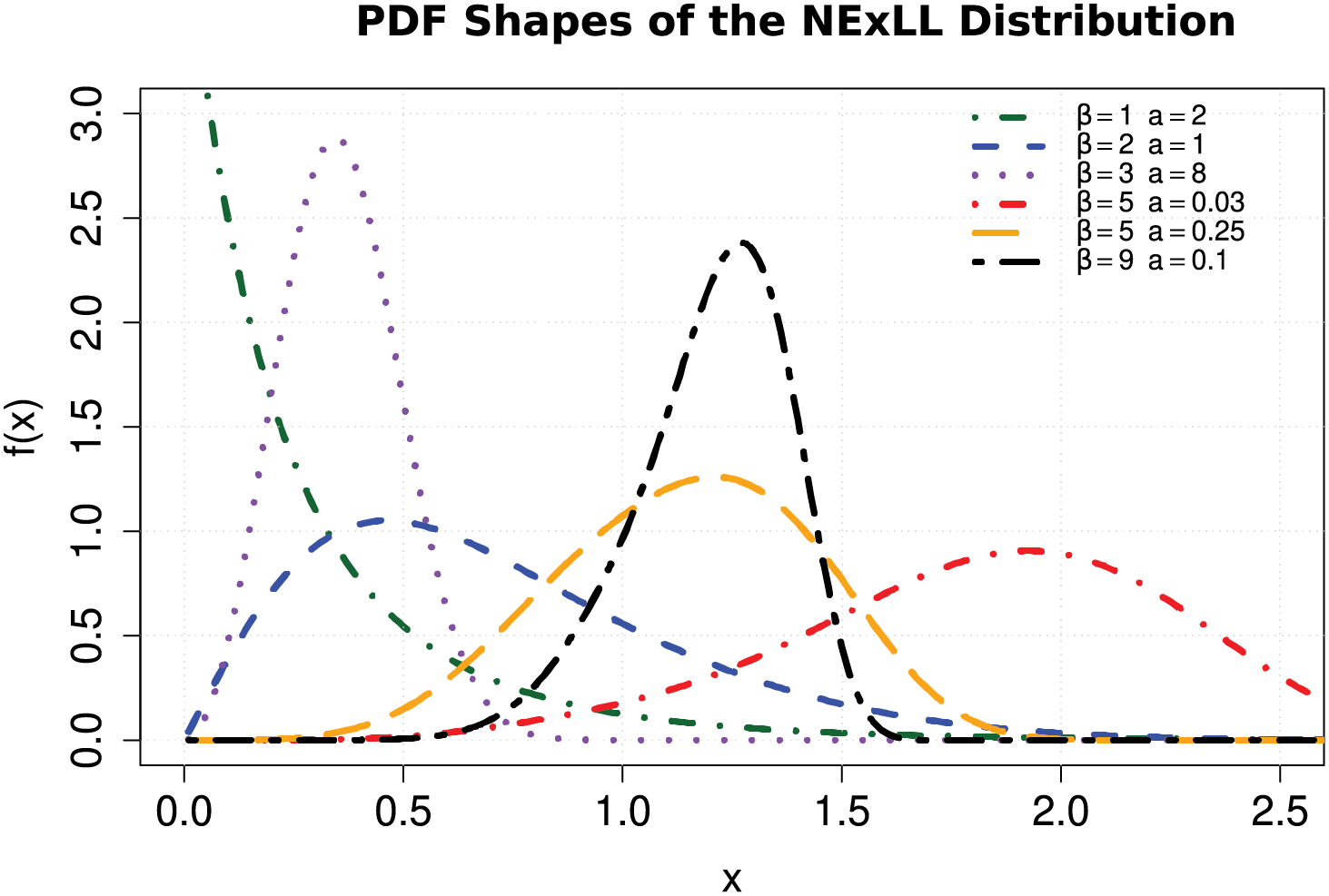
Figure 1: Some possible density shapes of the NExLL for various parametric values with λ=1

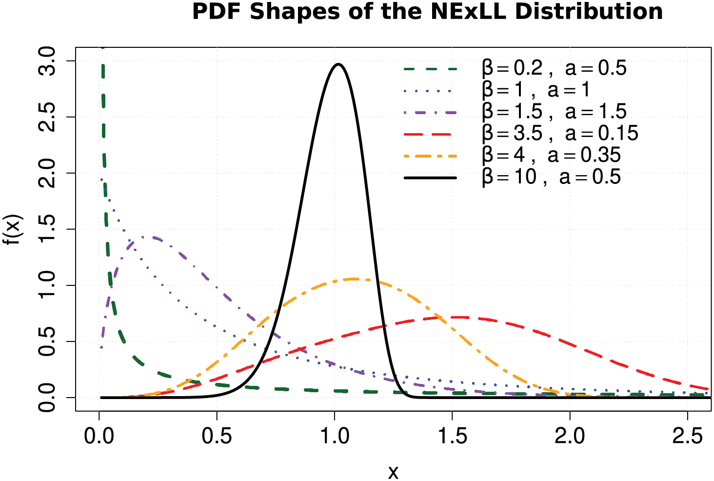
Figure 2: Some possible density shapes of the NExLL for various parametric values with λ=1

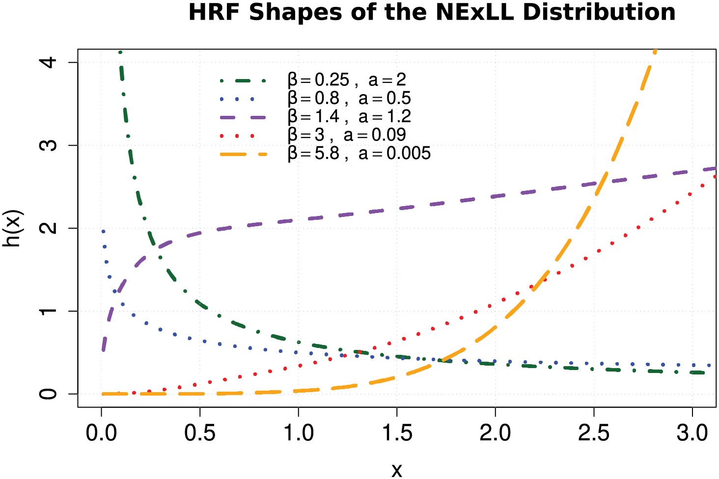
Figure 3: Some possible failure rate shapes of the NExLL for various parametric values with λ=1

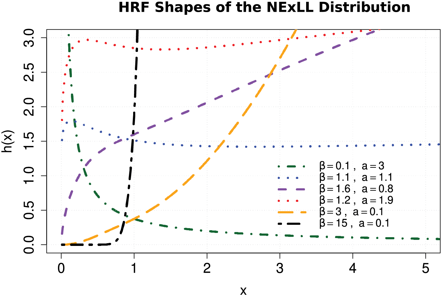
Figure 4: Some possible failure rate shapes of the NExLL for various parametric values with λ=1

3  Properties of the NExLL Distribution

3.1 Linear Representation

To improve interpretability, we begin by deriving a series representation of the NExLL distribution. This representation expresses the density as a weighted infinite sum of simpler exponentiated-LL (ELL) components, which facilitates theoretical development and practical computation.

A useful mixture representation of the PDF of the NEx-G class was provided in [10]. According to the NEx-G density reduces to

f(x)=∑i,j,k=0∞(−a)i(−1)k+1i!(k+i)g(x)G(x)i+k−1(ij)(j−ik).

By substituting the PDF and CDF of the LL model into the general NEx-G formulation, we derive the expanded form of the NExLL density. This expression, although complex, captures the flexible structure of the model through a combination of LL components. After some algebra, the NExLL density takes the form:

f(x)=∑i,j,k=0∞(−a)i(−1)k+1λβx−β−1i!(k+i)(1+λxβ)−2(1+λxβ)1−i−k(ij)(j−ik).

For computational efficiency and theoretical tractability, this expression can be rewritten as a more compact infinite sum involving ELL densities, each scaled by specific weight coefficients τi,k, as follows:

f(x)=∑i,k=0∞τi,kξk+i(x),(8)

where ξk+i(x)=(k+i)g(x)(G(x))k+i−1 is the ELL density with power parameter and (k+i)>0, and

τi,k=∑j=0∞(−a)i(−1)k+1i!(ij)(j−ik).

3.2 Some Moments

Using the linear representation, we derive the moments of the NExLL distribution by evaluating the weighted integrals of ELL components. This approach simplifies the calculation of moments by leveraging known results for the ELL distribution.

The r-th moment of X can be obtained from Eq. (8) as

μr′=E(Xr)=∑i,k=0∞τi,k∫0∞xrξk+i(x)dx.

Hence, we have

μr′=∑i,k=0∞τi,kλβ(k+i)∫0∞xr−β−1 (1+λxβ)−i−k−1dx.

After performing the integration, we obtain a closed-form series expression for the rth moment, which is valid under the condition rβ<1 to ensure convergence. Hence, we have

μr′=∑i,k=0∞τi,kλrβ(k+i)Γ(1−rβ) Γ(rβ+k+i)Γ(k+i+1), rβ<1.(9)

The mean of X, say, μX, follows from (9) with r=1.

Similarly, the rth incomplete moment is computed by integrating the density function up to a threshold t. The resulting expression involves the hypergeometric function F12, commonly encountered in survival analysis and income distribution studies.

The rth incomplete moment of the NExLL distribution has the form

Ir(t)=∫0txrf(x)dx.

Using Eq. (8), Ir(t) reduces to

Ir(t)=∑i,k=0∞τi,k∫0txrξk+i(x)dx.

Then, we obtain

Ir(t)=τi,kλβ tr−β(k+i) β−rF12(−rβ+1,k+i+1;−rβ+2;−λtβ),

where F12(−rβ+1,k+i+1;−rβ+2;−λtβ) is the hyper geometric function.

The mean residual life of the NExLL distribution at age t has the form

ψ(t)=1−I1(t)S(t)−t=∑i,k=0∞(β−1)−τi,kϕi,kλβ tr−β(k+i)(β−1)[e−a(ω[2−ω]1−ω)−t],

where ω=(1+λtβ)−1,ϕi,k=2F1(−1β+1,k+i+1;−1β+2;−λtβ) and I1(t) is the first incomplete moments.

The mean inactivity time of the NExLL distribution takes the form

φ(t)=t−I1(t)F(t)=t−τi,kϕi,kλβ(k+i)(β−1)[e−a(ω[2−ω]1−ω)−t].

The Lorenz (L) [35], Bonferroni (B), and Zenga (Z) curves are among the most important tools for measuring inequality, with notable applications in fields such as insurance, medicine, reliability, and economics.

The Lorenz (L) [35], Bonferroni (B) and Zenga (Z) curves are considered the most important inequality curves and have some applications in insurance, medicine, reliability, and economics.

The L curve is defined for the KAPLL distribution as follows:

L(p)=I1(xp)μ1′=∑i,k=0∞ϕi,kλ1−1ββ xp1−βΓ(k+i+1)(β−1)Γ(1−1β) Γ(1β+k+i),

where ϕi,k=F12(−1β+1,k+i+1;−1β+2;−λtβ) and I1(t) is the first incomplete moments.

The B and Z inequality curves can be determined, through their relationship with the L curve, by the following formulae [36]

B(p)=L(p)pandZ(p)=L(p)−pp[1−L(p)].

The moment generating function (MGF) can also be derived using the linear representation, which leads to a nested summation form involving gamma functions. This function can be used to derive higher-order moments and cumulants.

The MGF of the NExLL model is defined by

M(t)=E(etx)=∫−∞∞etx f(x) dx.

Based on Eq. (8), we can write

M(t)=∑i,k=0∞τi,k∫0∞etxξk+i(x)dx.

The MGF of the NExLL follows, after some algebra, as

M(t)=∑i,k,s=0∞τi,ktsλsβ(k+i) Γ(1−sβ) Γ(sβ+k+i)s!Γ(k+i+1), sβ<1. 

Table 1 presents the computed values of μX using both the truncated series summation (SUM) formula and numerical integration (NI) for various combinations of β, a, and fixed λ=1. The results indicate that as the number of terms M increases, the SUM values converge and stabilize, closely approximating the corresponding NI values. This convergence behavior confirms the accuracy and efficiency of the proposed SUM formula in estimating μX, particularly for M≥15, where the difference from the NI results becomes negligible across all parameter settings.

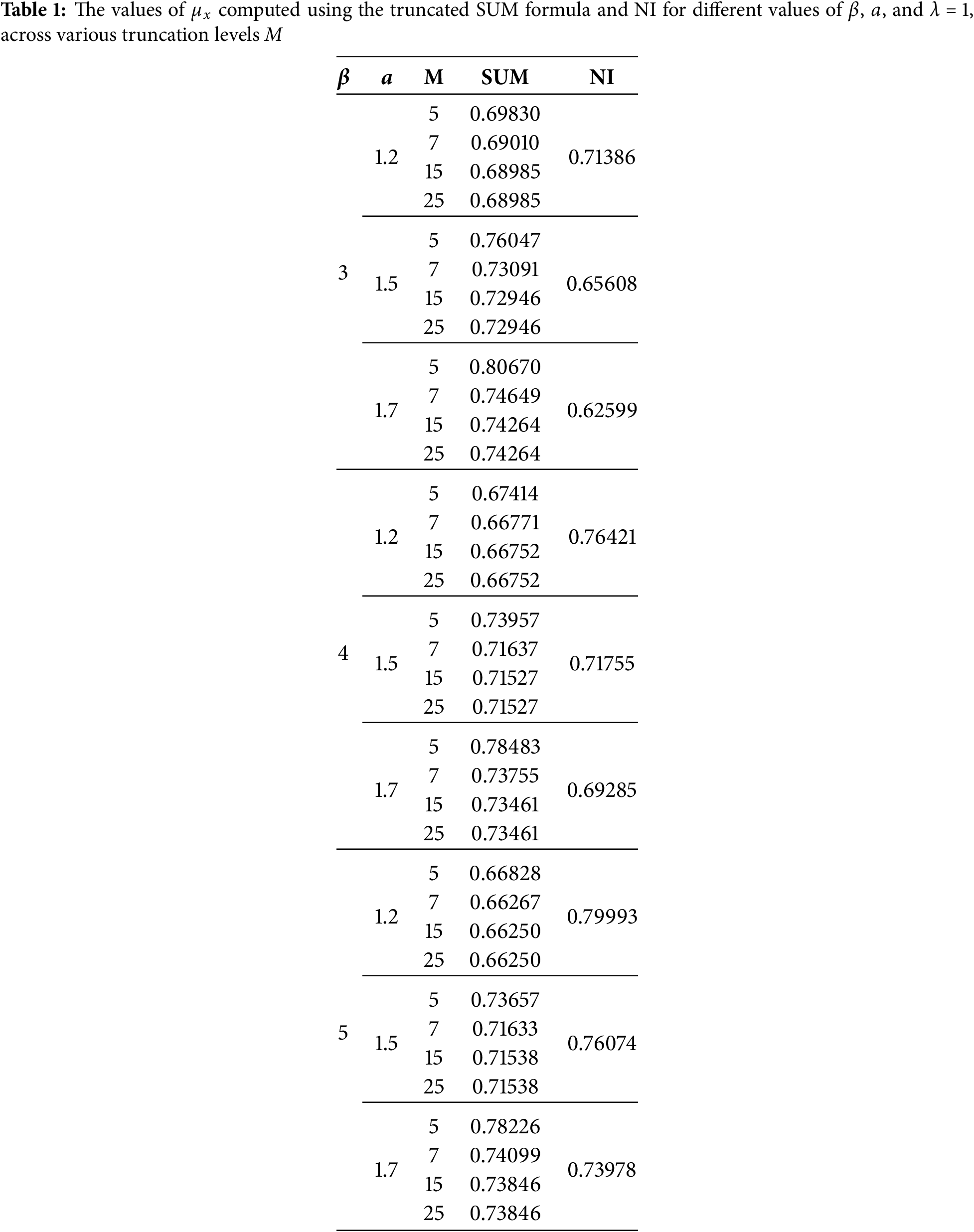
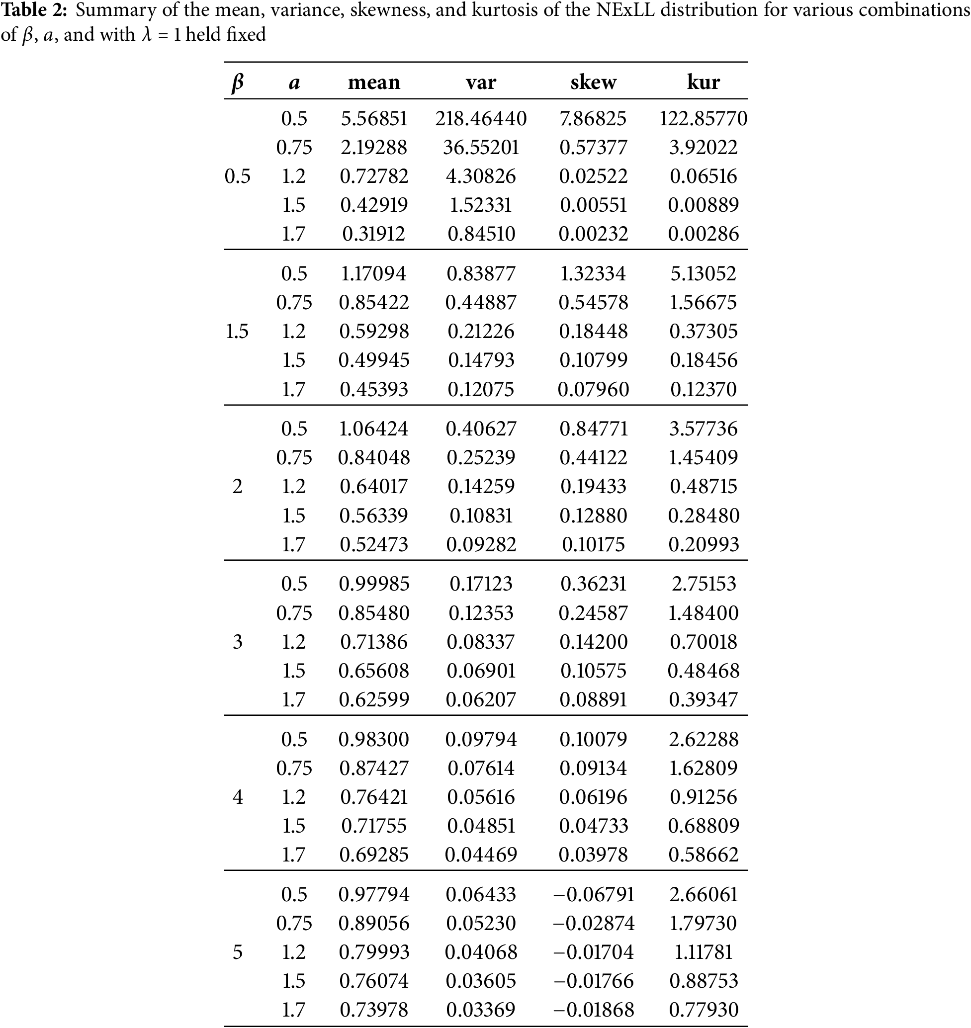
Table 2 presents key descriptive measures—mean μX, variance (var), skew, and kur—for the NExLL distribution across various combinations of the shape parameters β, a, with λ fixed at 1. These results are obtained using the R software, and reveal that as a increases for fixed β, both the mean and variance decrease significantly, indicating a shift toward more concentrated distributions. Additionally, the skewness and kurtosis measures decline with increasing a, suggesting a transition from highly skewed and heavy-tailed distributions (particularly at low a) to more symmetric and light-tailed forms. For higher values of β, some negative skewness appears, indicating the model’s flexibility in capturing left-skewed behavior as well. These findings demonstrate the strong adaptability of the NExLL distribution to various data patterns, especially in modeling dispersion and tail behavior.

3.3 Rényi and m-Entropies

Measures of entropy, such as Rényi and m-entropies, quantify the uncertainty of the NExLL model. These are obtained by raising the PDF to a power m and integrating, again using the linear expansion to express the result as a tractable summation.

The Rényi entropy of a random variable X is defined by

PX(m)=11−mlog⁡∫0∞fm(x)dx,m>0,m≠1.

Using Eq. (8), the Rényi entropy of the NExLL model takes the form

PX(m)=11−mlog⁡[∑k=0∞τi,kmβm−1λ1−mβ(k+i)mΓ(βm[k+i]−m+1β)Γ(m[1+β]−1β)Γ(m(k+i+1))].(10)

The m−entropy, say, LX(m), is defined by

LX(m)=1m−1log⁡[1−∫0∞fm(x)dx],m>0,m≠1.

Hence, using (10), the m−entropy of the NExLL model follows as

LX(m)=1q−1log⁡[1−∑k=0∞τi,kmβm−1λ1−mβ(k+i)mΓ(βm[k+i]−m+1β)Γ(m[1+β]−1β)Γ(m(k+i+1))].

3.4 Order Statistics

The order statistics of the NExLL distribution are derived from its PDF and CDF. Given the series form of the density, the order statistic distributions also naturally take the form of infinite summations over ELL components.

Let X1, X2, … , Xn be a random sample of size n and let X1:n,…,Xn:n be their associated order statistic. Then, the PDF of the ith order statistics, say, Xi:n, which is denoted by fXi:n(x), reduces to

fXi:n(x)=n!f(x)(n−i)!(i−1)![F(x)]i−1[1−F(x)]n−i.(11)

Substituting (5) and (6) in (11), the ith order statistic of the NExLL distribution follows as

fXi:n(x)=n!(n−i)!(i−1)!(∑i,k=0∞di,k)s+n−i+1∑s=0∞(i−1s)(−1)sπi+k(x)×[G(x)i+k](s+n−i),(12)

where di,k=∑j=0∞(−a)i(−1)ki!(ij)(j−ik), πi+k(x)=(i+k) g(x) G(x)i+k−1, G(x) and g(x) are given by Eqs. (1) and (2), respectively.

After some algebra, we obtain

fXi:n(x)=∑i,k,s=0∞n!(−1)s(i+k)[di,k]s+n−i+1(n−i)!(i−1)! g(x) G(x)(i+k)(s+n−i+1)−1(i−1s).

The last equation can be expressed as

fi:n(x)=∑s=0∞ws hs+1(x),

where hs+1(x)=(i+k)(s+n−i+1)g(x) G(x)(i+k)(s+n−i+1)−1 is the exponentiated-LL density with power parameter (i+k)(s+n−i+1)>0, and

ws=∑i,k=0∞n!(−1)s[di,k]s+n−i+1(n−i)!(i−1)!(s+n−i+1)(i−1s).

4  Estimation Methods

In this section, we use seven methods to estimate the NExLL parameters namely: the maximum likelihood (ML), least-squares (LS), weighted LS (WLS), maximum product of spacings (MPS), Cramér–von Mises (CRVM), Anderson–Darling (AD), and right-tail AD (RAD) methods.

Let x1,x2,…,xn be a random sample from NExLL distribution then the logarithm of the likelihood function, say, (ℓ), becomes

ℓ=n(ln⁡a+ln⁡β−ln⁡λ)+(β−1)∑i=1nln⁡xi+∑i=1nln⁡(1+λ2ϑi2 )−a∑i=1nxiβ(ϑi+λ)λϑi,

where ϑi=xiβ+λ.

To estimate the parameters of the NExLL distribution, we derive the score functions corresponding to the log-likelihood function. These score functions, defined as the partial derivatives of the log-likelihood with respect to the parameters a, λ and β, are solved simultaneously to obtain the MLE. The explicit expressions for the score functions are given below.

∂ℓ∂a=na−∑i=1nxiβ(ϑi+λ)λϑi,∂ℓ∂λ=−nλ+∑i=1n(1+λ2ϑi2)−12λxiβϑi3−a∑i=1n2λxiβϑi−xiβ(ϑi+λ)2λ2ϑi2

and

∂ℓ∂β=nβ+∑i=1nln⁡(xi)−∑i=1n(1+λ2ϑi2)−12λ2xiβln⁡(xi)ϑi3−a∑i=1nλϑi(2xi2βln⁡(xi)+2λxiβln⁡(xi))−(λxiβln⁡(xi)[xi2β+2λxiβ])λ2ϑi2.

The LSE and WLSE of the NExLL parameters β, λ and a and can be obtained by minimizing

O(α,β,λ,a,b)=∑i=1nνi[F(xi:n) −in+1]2,

where νi =1 in case of the LSE approach and νi=(n+1)2(n+2)/[i(n−i+1)] in case of the WLSE approach.

The LS and WLS estimators are obtained by solving the following nonlinear estimating equations:

∑i=1n{1−exp⁡[−axi:nβ(ϑi:n+λ)λϑi:n]−in+1}δs(xi:n)=0, s=1,2,3,

where δ1(xi:n), δ2(xi:n), and δ3(xi:n) denote the partial derivatives of the CDF with respect to a, λ and β, respectively. These are given as:

δ1(xi:n)=∂F(xi:n)∂a=xi:nβ(xi:nβ+2λ)λ(xi:nβ+λ)exp⁡{−axi:nβ(xi:nβ+2λ)λ(xi:nβ+λ)}.

Let ϑi:n=xi:nβ+λ, then the above equation simplifies to:

δ1(xi:n)=xi:nβ(ϑi:n+λ)λϑi:nexp⁡[−axi:nβ(ϑi:n+λ)λϑi:n],(13)

δ2(xi:n)=∂F(xi:n)∂λ=2aλxi:nβ(xi:nβ+λ)−axi:nβ(xi:nβ+2λ)2λ2(xi:nβ+λ)2exp⁡{−axi:nβ(xi:nβ+2λ)λ(xi:nβ+λ)}.

Using ϑi:n, the last equation reduces to:

δ2(xi:n)=2aλxi:nβϑi:n−axi:nβ(xi:nβ+2λ)2λ2ϑi:n2exp⁡[−axi:nβ(ϑi:n+λ)λϑi:n],(14)

and

δ3(xi:n)=∂F(xi:n)∂β=exp⁡{−axi:nβ(xi:nβ+2λ)λ(xi:nβ+λ)}×a(λ(xi:nβ+λ)[2xi:n2βln⁡(xi:n)+2λxi:nβln⁡(xi:n)])−a(λxi:nβln⁡(xi:n)[xi:n2β+2λxi:nβ])λ2(xi:nβ+λ)2.

Using ϑi:n and letting ηi:n=xi:nβln⁡(xi:n) and ϑi:n=xi:nβ+λ, the equation above can be rewritten as:

δ3(xi:n)=a(λϑi:n[2xi:nβηi:n+2ληi:n])−a(ληi:n[xi:n2β+2λxi:nβ])λ2ϑi:n2exp⁡[−axi:nβ(ϑi:n+λ)λϑi:n].(15)

Note: In the above expressions, ϑi:n=xi:nβ+λ and ηi:n=xi:nβln⁡xi:n are auxiliary terms introduced to simplify notation. These derivatives are used in solving the estimating equations for the LS, WLS, MPS, CRVM, AD, and RAD methods.

The MPSE is an alternative approach to the MLE [37,38]. The uniform spacings of a random sample of size n from the NExLL distribution ar defined by

H(β,λ,a,)=∑i=1n+1log⁡[Di],

where Di=Di(β,λ,a,)=F(xi:n)−F(xi−1:n) be the uniform spacing for (i=1,…,n+1), where F(x(0))=0,F(x(n+1))=1 and ∑i=1n+1Di=1.

The MPSE of the NExLL parameters are determined by solving the non-linear equations

∑i=1n+11Diδs(xi:n)−δs(xi−1:n)=0,s=1,2,3,

where δs(xi:n)=0 are defined in (13)–(15) for s=1,2,3.

The CRVM method minimizes the integrated squared difference between the theoretical and empirical CDFs. The CRVME of the NExLL parameters are obtained by minimizing the following objective function:

C(β,λ,a,)=112n+∑i=1n{1−exp⁡[−axi:nβ(ϑi:n+λ)λϑi:n]−2i−12n}2,

which also follow by solving the following estimating equations:

∑i=1n{1−exp⁡[−axi:nβ(ϑi:n+λ)λϑi:n]−2i−12n}δs(xi:n)=0, s=1,2,3.

The AD method places more weight on the tails of the distribution. The ADE of the NExLL parameters are obtained by minimizing

A(β,λ,a,)=−n−1n+∑i=1n(2i−1)[log⁡F(xi:n) +log⁡S(xi:n)],

where S(xi:n)=1−F(xi:n).

The ADE can also be found as solutions of the following estimating equations:

∑i=1n(2i−1)[δs(xi:n)F(xi) +δi(xn+1−i:n)S(xn+1−i:n)]=0, s=1,2,3.

The RAD method is a one-sided modification of the AD method focusing on the right tail. The RADE of the NExLL parameters β, λ and a are obtained by minimizing the following function:

R(β,λ,a)=1n−2∑i=1nF(xi:n)−1n∑i=1n(2i−1)log⁡S(xn+1−i:n).

They can also be obtained from the non-linear estimating equations:

−2∑i=1nδS(xi:n)+1n∑i=1n(2i−1)δS(xn+1−i:n)/S(xn+1−i:n)=0, s=1,2,3,

where the expressions δs(xi:n) are the partial derivatives of the CDF F(x) with respect to the parameters a, λ, and β, defined as:

δ1(xi:n)=∂F(xi:n)∂a,δ2(xi:n)=∂F(xi:n)∂λ,δ3(xi:n)=∂F(xi:n)∂β.

Each of these derivatives is given explicitly in Eqs. (13)–(15), and they are used throughout all estimating equations presented above.

In summary, the score and estimating equations for all seven estimation methods have been explicitly derived, clearly labeled, and organized for better readability. These formulations provide practitioners with the tools necessary to implement the methods and ensure reproducibility of results.

5  Numerical Simulations

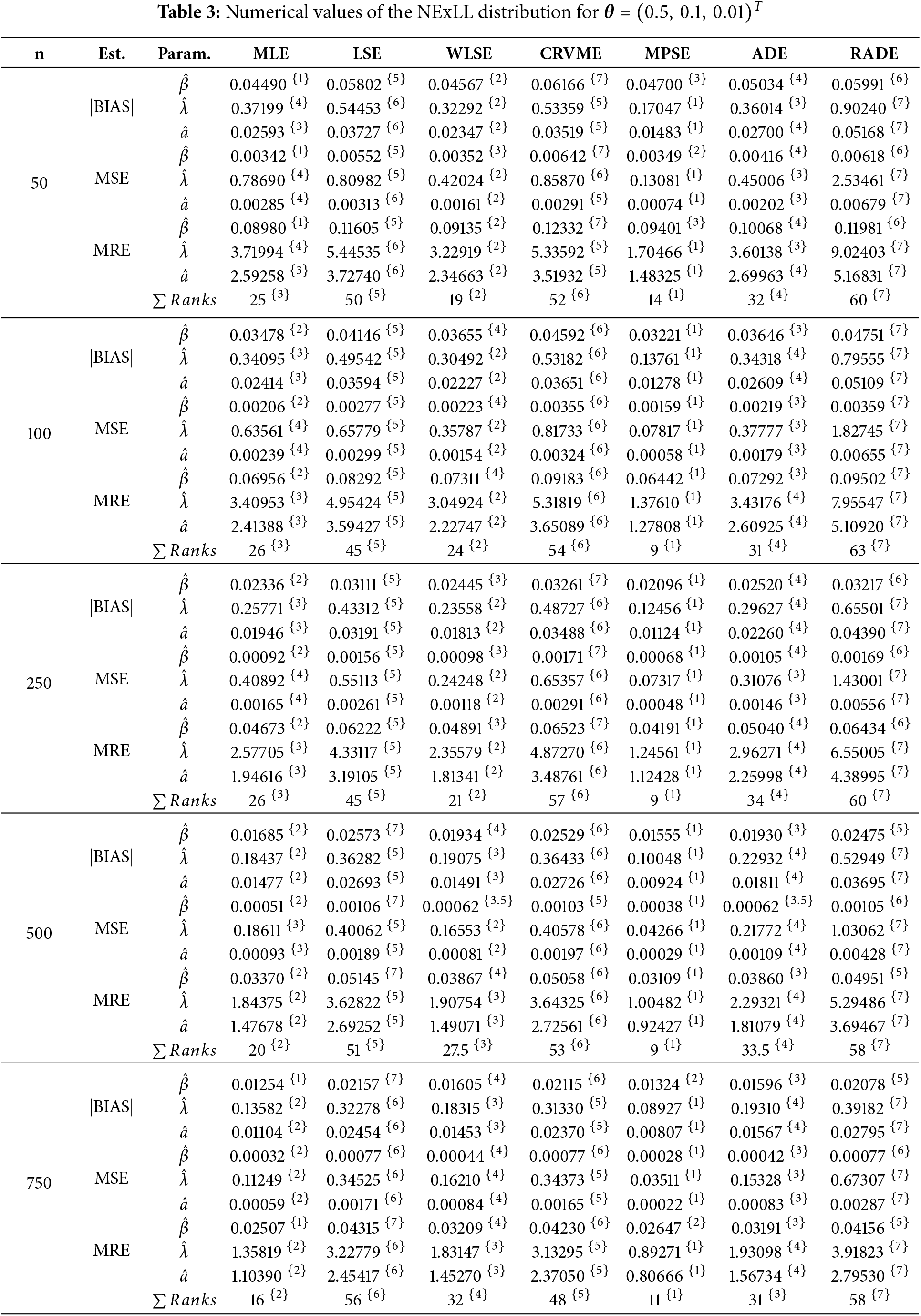
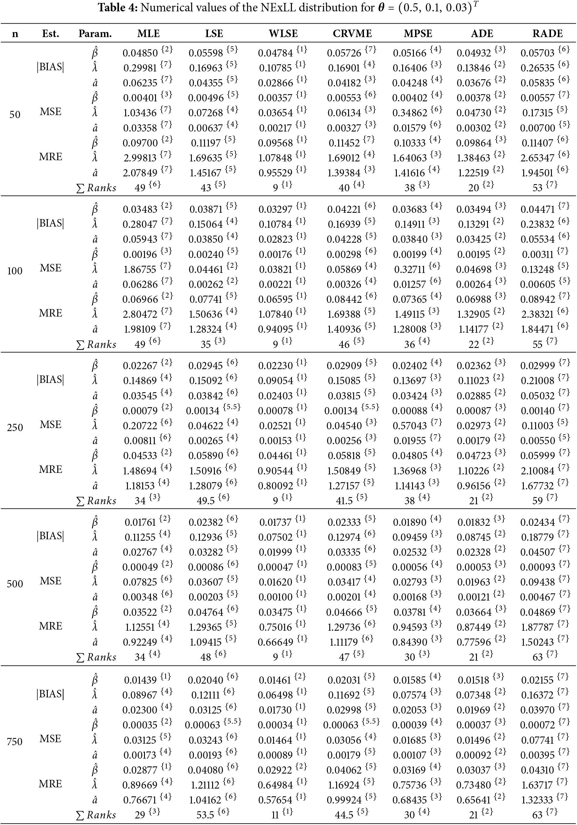
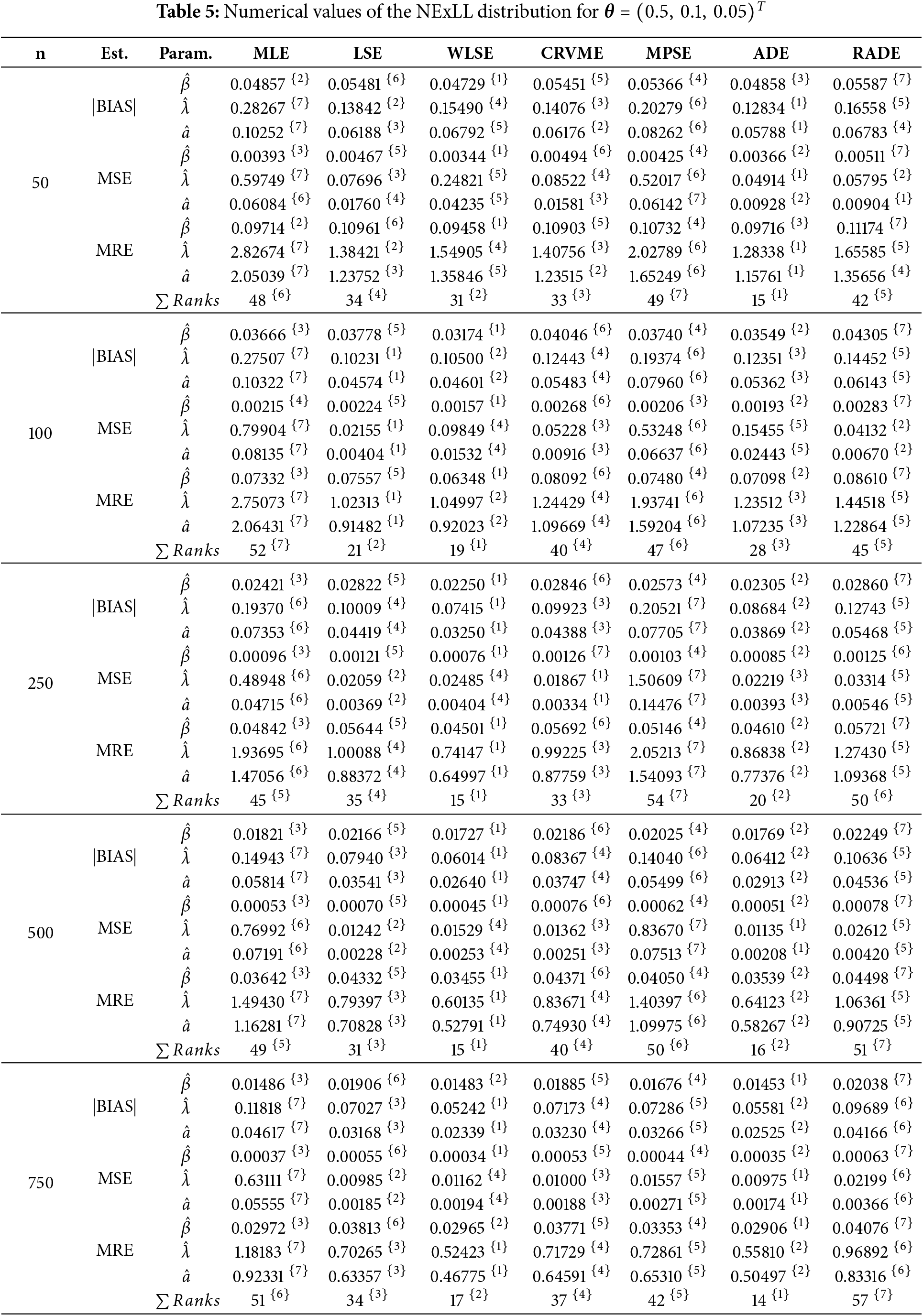
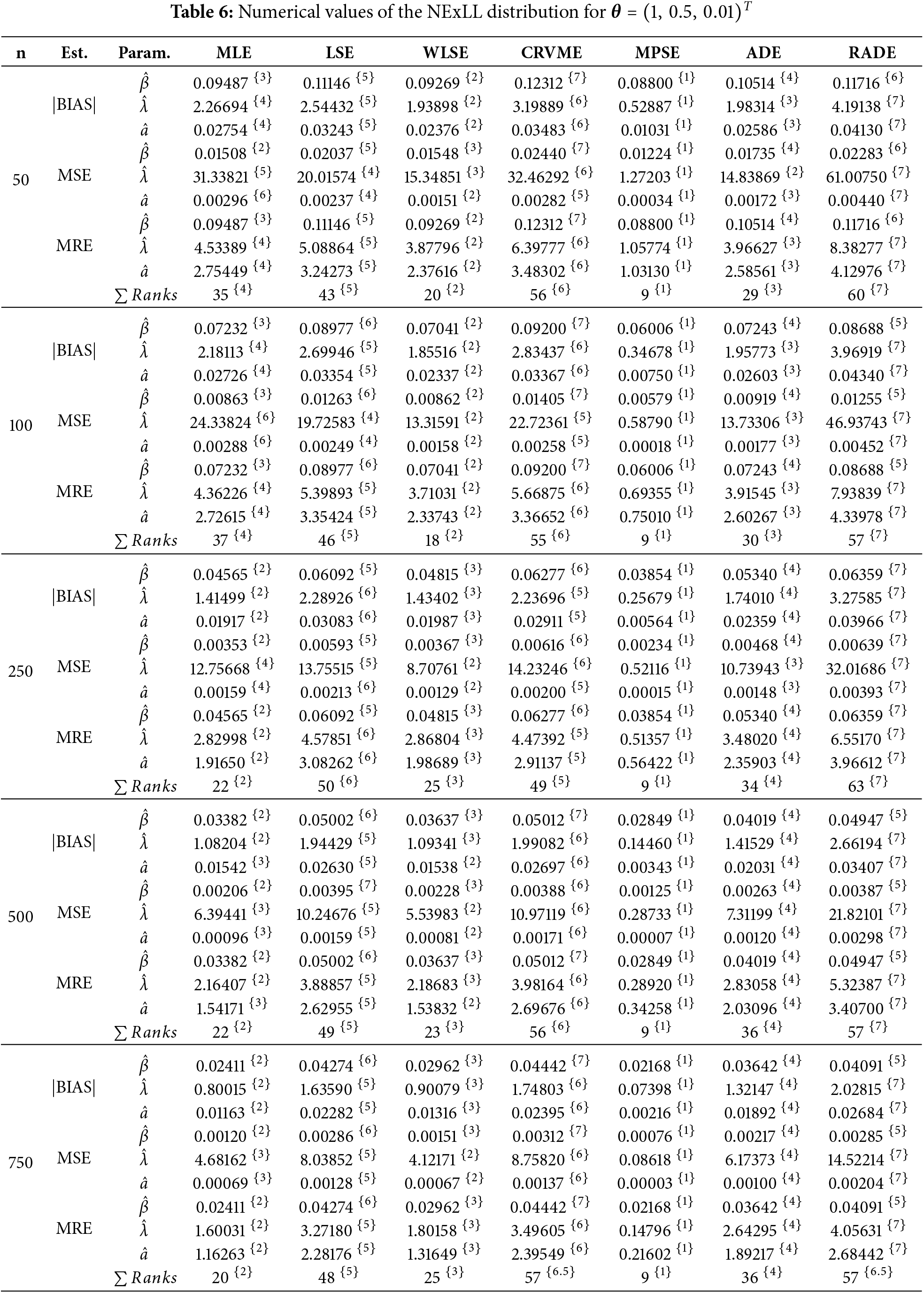
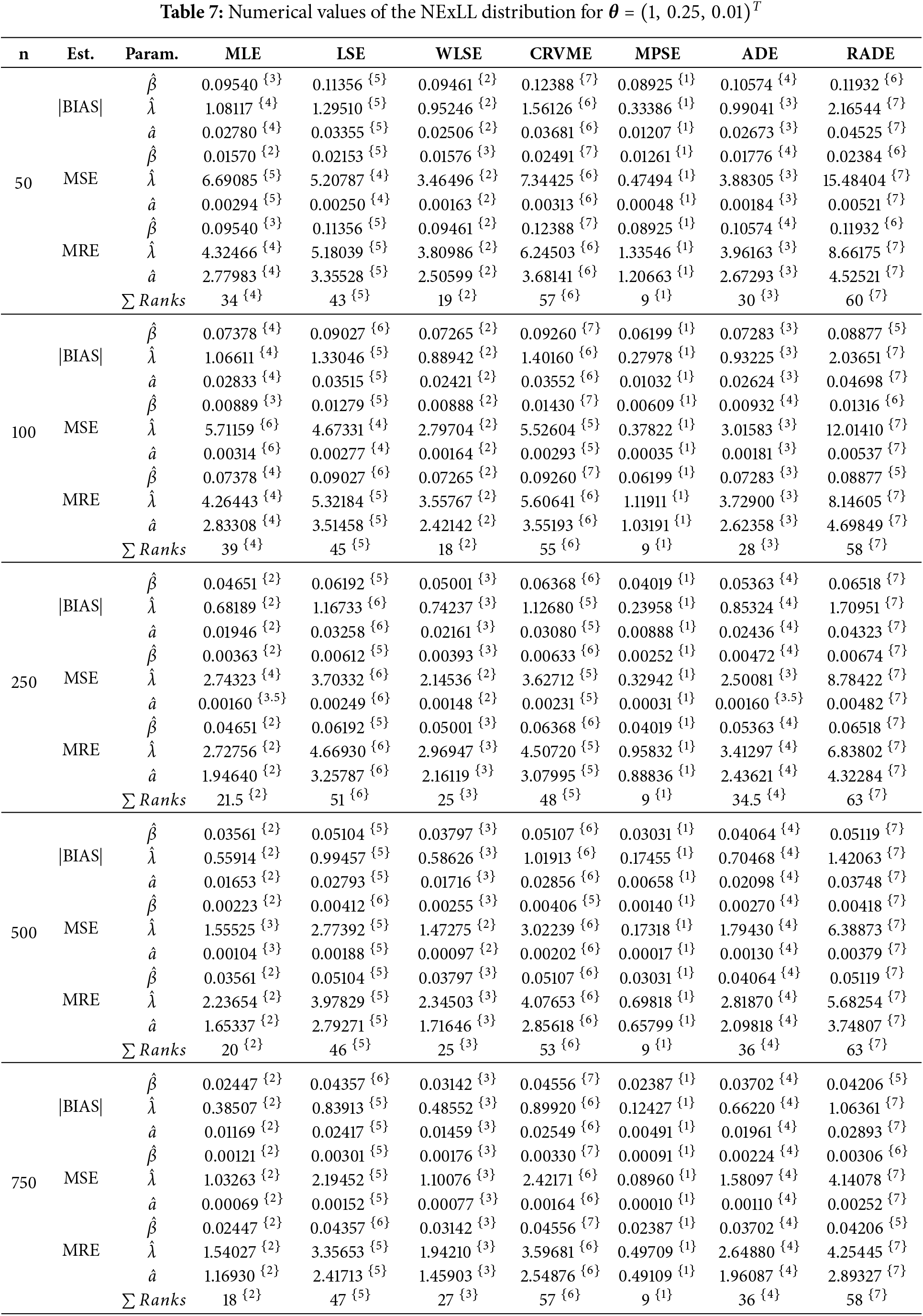
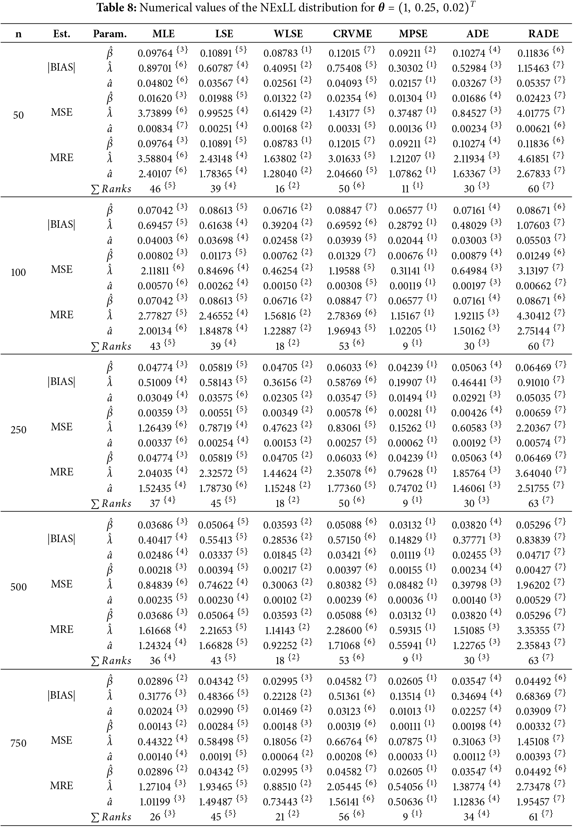
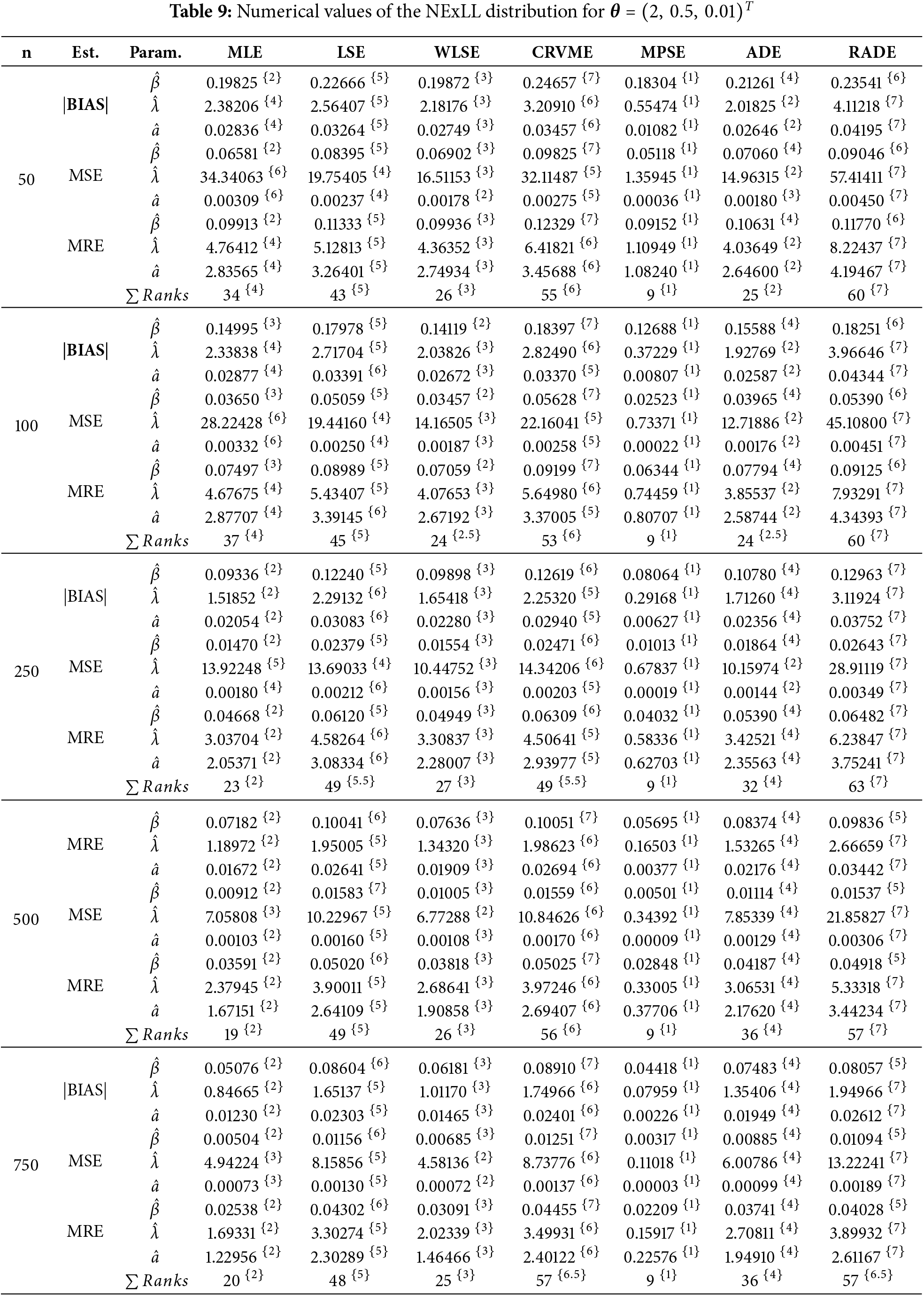
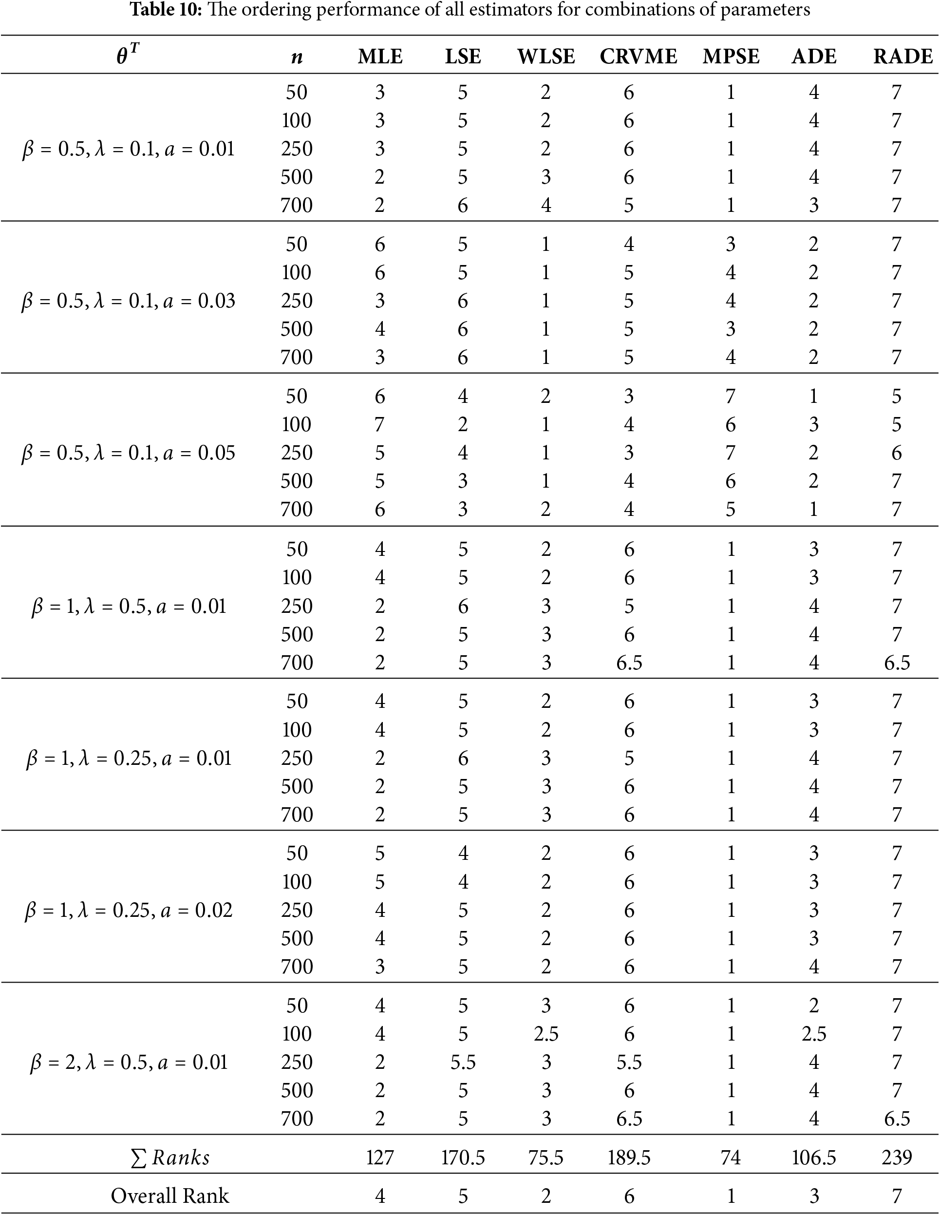
This sections gives detailed simulation results to explore the behavior and performances of the introduced estimation methods in estimating the NExLL parameters based on the following three measures namely: the mean square errors (MSE), MSE =1N∑i=1N(θ^−θ)2, average absolute biases (|BIAS|), |BIAS| =1N∑i=1N|θ^−θ|, and mean relative errors (MRE), MRE =1N∑i=1N|θ^−θ|/θ, where θ=(β,λ,a)T.

Several sample sizes and parameters combinations are considered, i.e., n = {50, 100, 250, 500, 750}, θ=(0.5,0.1,0.01)T, θ=(0.5,0.1,0.03)T, θ=(0.5,0.1,0.05)T, θ=(1,0.5,0.01)T, θ=(1,0.25,0.01)T, θ=(1,0.25,0.02)T, θ=(2,0.5,0.01)T. We generated N=1000 random samples based on the QF in (7) using the R software.

Tables 3–10 give the findings of simulations including the |BIAS|, MSE, and MRE for the eight estimation approaches. The results show that the values of |BIAS|, MSE and MRE decrease with the increase of n, showing that the given estimators are consistent. Hence, the introduced estimation methods perform very well in estimating the NExLL parameters. Generally, based on simulation results, the ordering performance of the estimators is as follows: MPSE, WLSE, ADE, MLE, LSE, CRVME, and RADE. This order confirms the superiority of the MPS estimation method with overall sore of 74.

6  Real-World Data Applications

This section illustrates the importance and applicability of the NExLL distribution by fitting two real-life data applications from Reliability and engineering sciences. The first data set is addressed by [39], and it contains 40 observations of time to failure (103h) of turbocharger of one type of engine. The data are: 3.5, 1.6, 5.4, 4.8, 6.0, 7.0, 6.5, 7.3, 8.0, 7.7, 8.4, 3.9, 2.0, 5.0, 6.1, 5.6, 8.1, 6.5, 7.3, 7.1, 7.8, 2.6, 8.4, 4.5, 5.8, 5.1, 6.3, 7.3, 6.7, 7.7, 8.3, 7.9, 8.5, 4.6, 3.0, 5.3, 8.7, 6.0, 9.0, 8.8.

The second data set refers to breaking stress of carbon fibers in (Gba) for 100 observations, and it is studied by [40]. The data are: 0.39, 0.81, 0.85, 0.98, 1.08, 1.12, 1.17, 1.18, 1.22, 1.25, 1.36, 1.41, 1.47, 1.57,1.57, 1.59, 1.59, 1.61, 1.61, 1.69, 1.69, 1.71, 1.73, 1.80, 1.84, 1.84, 1.87, 1.89, 1.92, 2.0, 2.03, 2.03, 2.05, 2.12, 2.17,2.17, 2.17, 2.35, 2.38, 2.41, 2.43, 2.48, 2.48, 2.50, 2.53, 2.55, 2.55, 2.56, 2.59, 2.67, 2.73, 2.74, 2.76, 2.77, 2.79, 2.81, 2.81, 2.82, 2.83, 2.85, 2.87, 2.88, 2.93, 2.95, 2.96, 2.97, 2.97, 3.09, 3.11, 3.11, 3.15, 3.15, 3.19, 3.19, 3.22, 3.22, 3.27, 3.28, 3.31, 3.31, 3.33, 3.39, 3.39, 3.51, 3.56, 3.60, 3.65, 3.68, 3.68, 3.68, 3.70, 3.75, 4.20, 4.38, 4.42, 4.70, 4.90, 4.91, 5.08, 5.56.

The fits of the NExLL distributions is compared with some existing LL distributions namely: the alpha power transformed LL (APTLL) [28], Poisson Burr type X LL (PBXLL) [26], beta LL (BLL) [21], Weibull generalized LL (WGLL) by [41], McDonald LL (McLL) [23], additive Weibull lL (AWLL) [42], and LL distributions.

The performance of the fitted distributions is explored using some measures including the Akaike information criterion (AIC), consistent Akaike IC (CAIC), Hannan–Quinn IC (HQIC), Bayesian IC (BIC), (−ℓ), where ℓ the maximized log-likelihood, as well as some statistics include the Cramér–Von Mises (W∗), Anderson–Darling (A∗), Kolmogorov–Smirnov (KS) and the KS p-value (PV).

All numerical results in this section are calculated using the R software. Tables 11 and 12 present the goodness-of-fit (GOF) results for the proposed NExLL distribution alongside several competing LL-based models, applied to two real datasets. The evaluation is conducted using a comprehensive set of model selection criteria and goodness-of-fit statistics to ensure robust and meaningful comparisons.

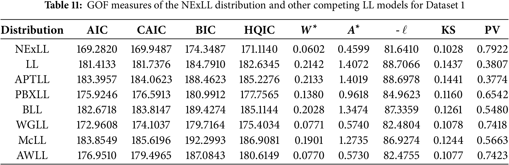
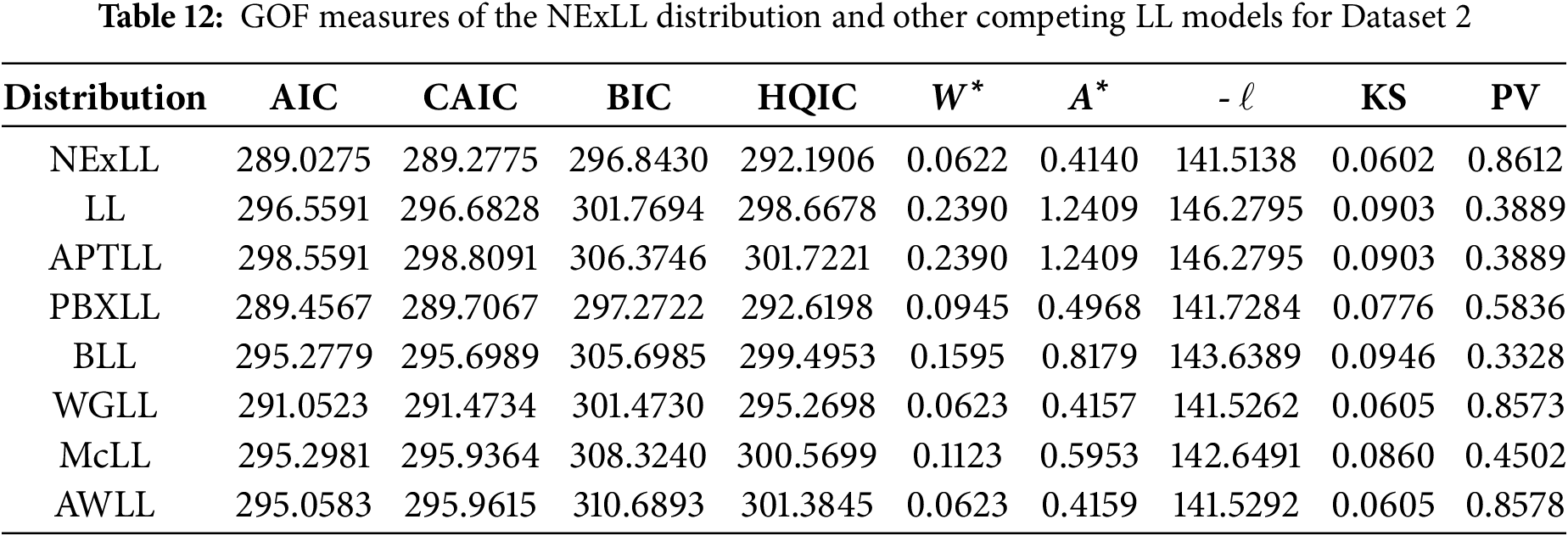
Specifically, the model selection criteria include the AIC, CAIC, HQIC, and BIC. These criteria assess the trade-off between model fit and complexity, where lower values generally indicate better-fitting models with fewer penalties for parameter count. Additionally, the statitic −ℓ reflects how well the model fits the data—lower values imply a better fit.

To evaluate the agreement between the empirical and theoretical distributions, we also report GOF statistics including W∗, A∗, and the KS statistic along with its corresponding PV. These statistics test the discrepancy between the empirical distribution function and the cumulative distribution function of the fitted model. Smaller values of W∗, A∗, and KS, and higher p-values, suggest a closer agreement between the model and observed data.

From Tables 11 and 12, it is evident that the NExLL distribution consistently achieves the lowest values for all considered information criteria and test statistics across both datasets. It also records the highest KS p-values, indicating no significant deviation from the empirical data. These results strongly support the superior flexibility and fitting capability of the NExLL model compared to other well-known and recently proposed LL-based distributions.

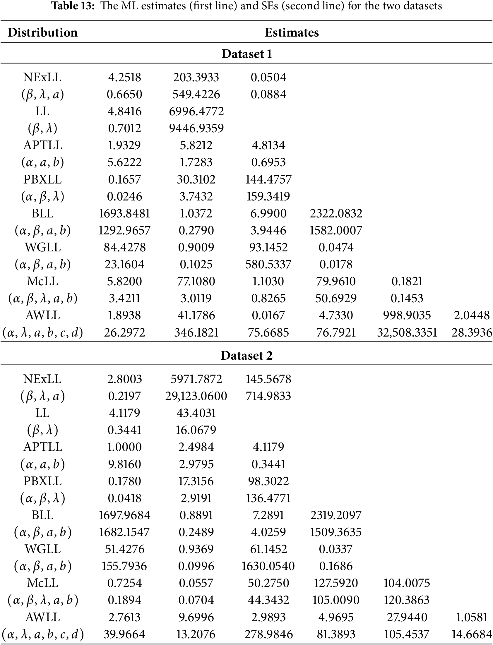
The ML estimates and standard errors (SEs) for the models’ parameters are reported in Table 13, for the two datasets. Overall, the NExLL distribution have the lowest values for goodness-of-fit criteria among all LL fitted models. Then, it could be chosen as the most adequate model for fitting the two datasets.

Furthermore, the visual fitting performance of the NExLL model is explored in Figs. 5 and 6. These figures show the histogram of the two data sets and the estimated PDFs, CDFs, SFs, and PP plots of the NExLL distribution. It is clear from these plots that the NExLL distribution provides the best fits to the two datasets.

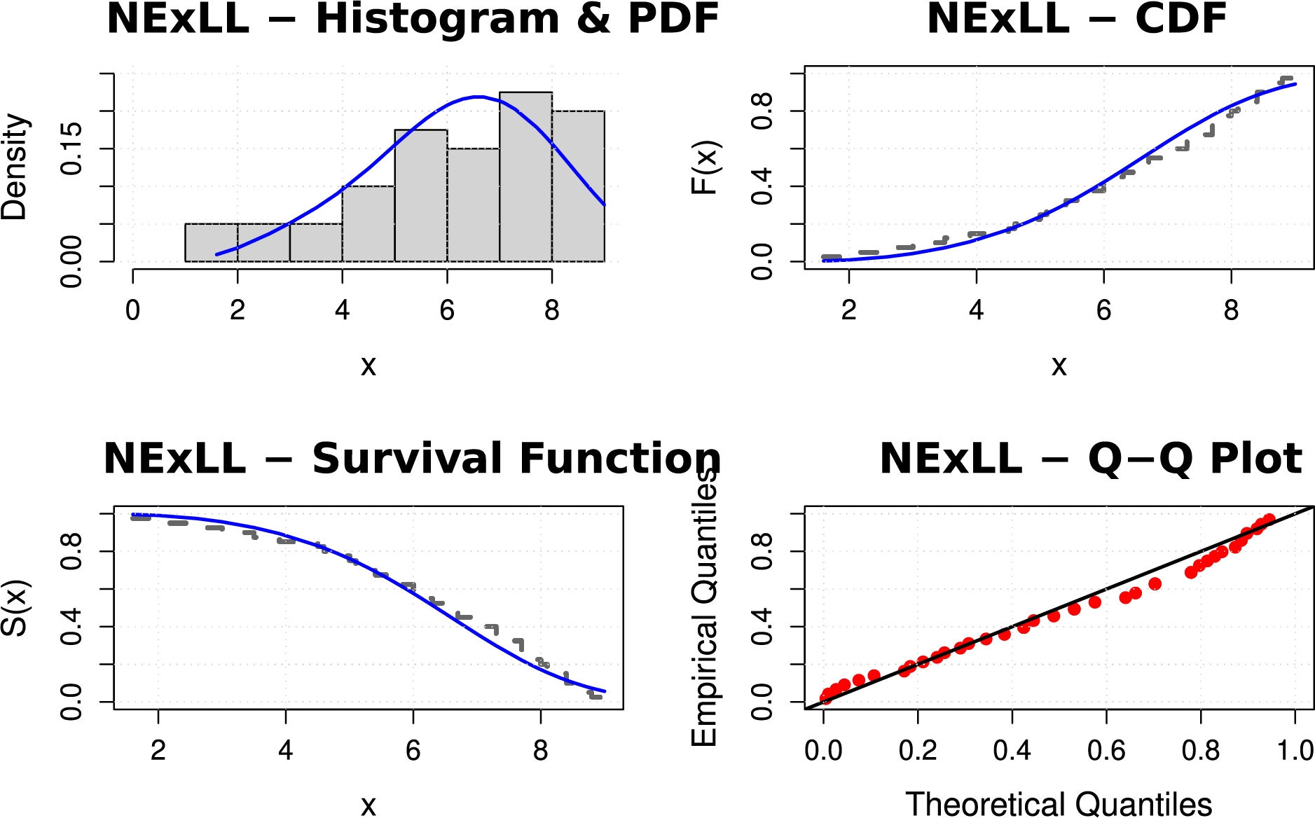
Figure 5: The fitted functions of the NExLL model for first dataset

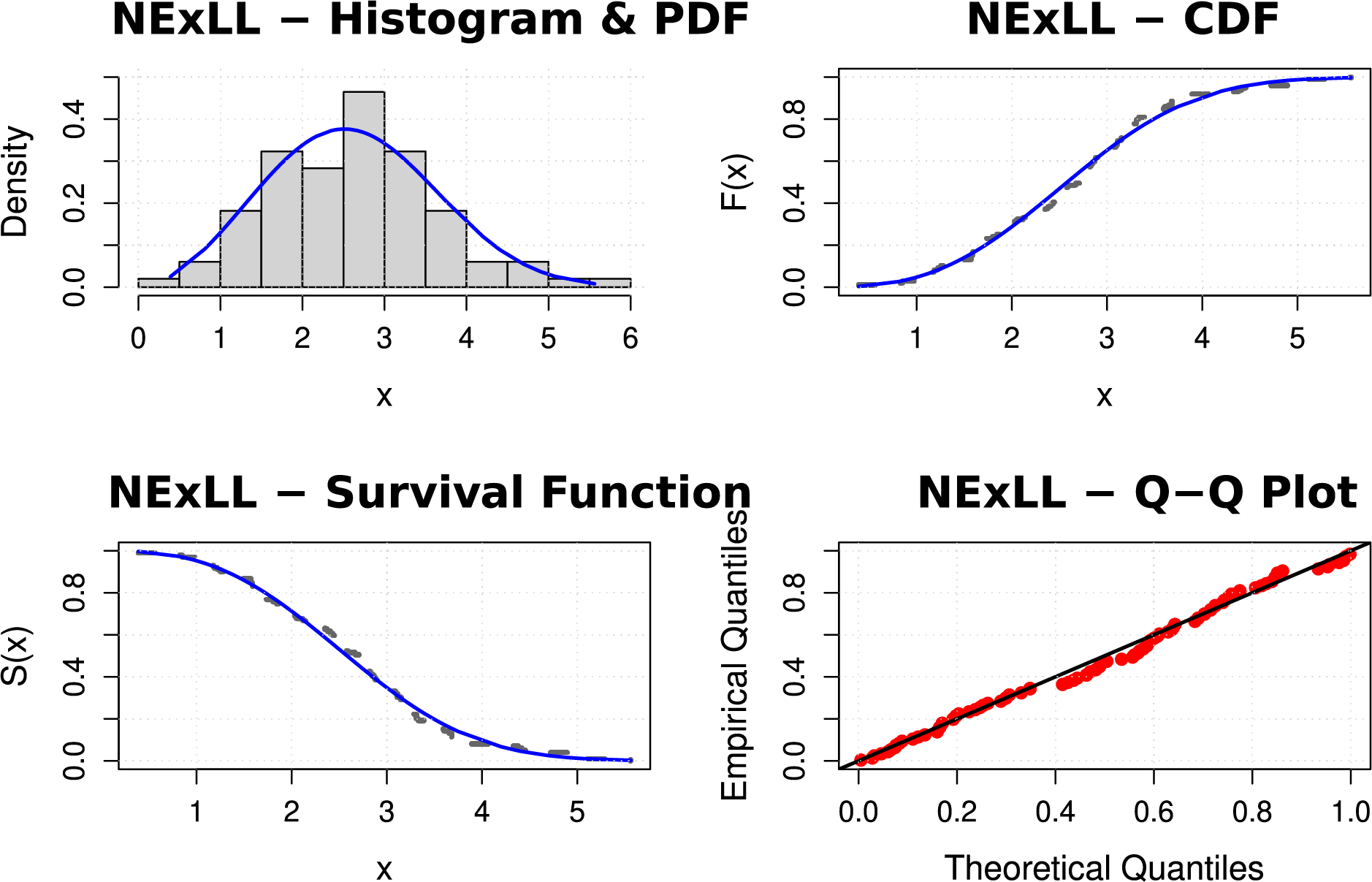
Figures 6: The fitted functions of the NExLL model for second dataset

Fig. 7 displays the histogram and corresponding fitted density curves for the two real-life datasets. The left panel illustrates the fit of the proposed NExLL distribution to the first dataset, while the right panel shows the fit for the second dataset. In both cases, the NExLL model closely follows the empirical data, capturing the underlying distributional patterns effectively. The visual alignment between the histograms and the fitted curves highlights the model’s flexibility and suitability for modeling real-world lifetime data with varying shapes and characteristics.

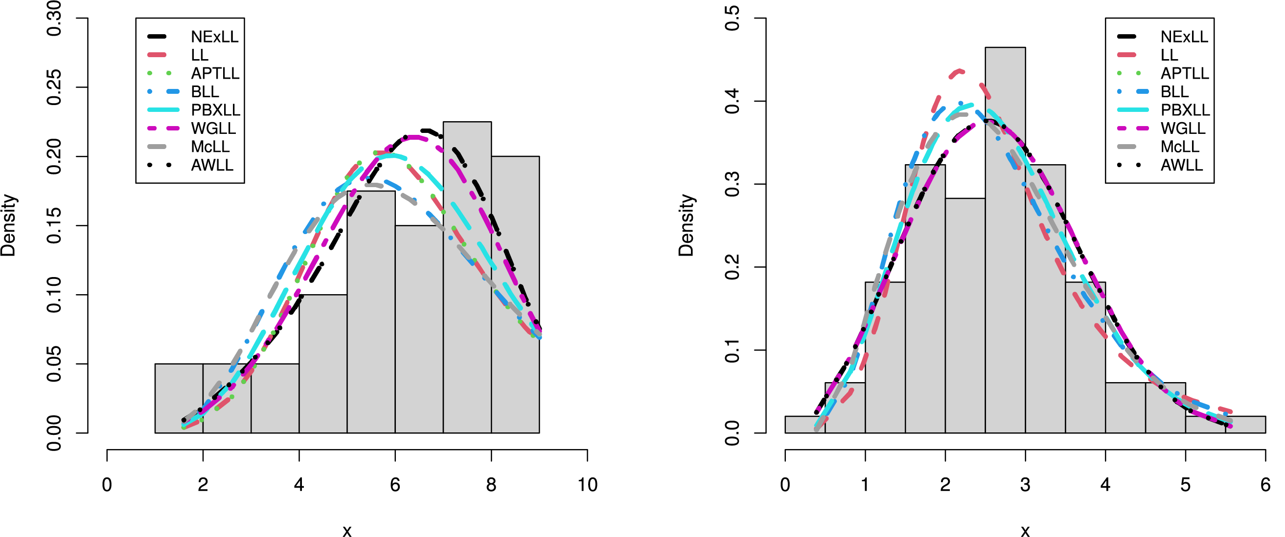
Figure 7: The histogram and fitted densities plots for the first dataset (left panel), and for the second dataset (right panel)

Additionally, the PP plots for the two datasets, presented in Figs. 8 and 9, confirm that the NExLL distribution provides a superior fit compared to competing distributions. The results demonstrate that the NExLL distribution consistently outperforms other LL extensions across all datasets, reinforcing its practical applicability for modeling real-world data.

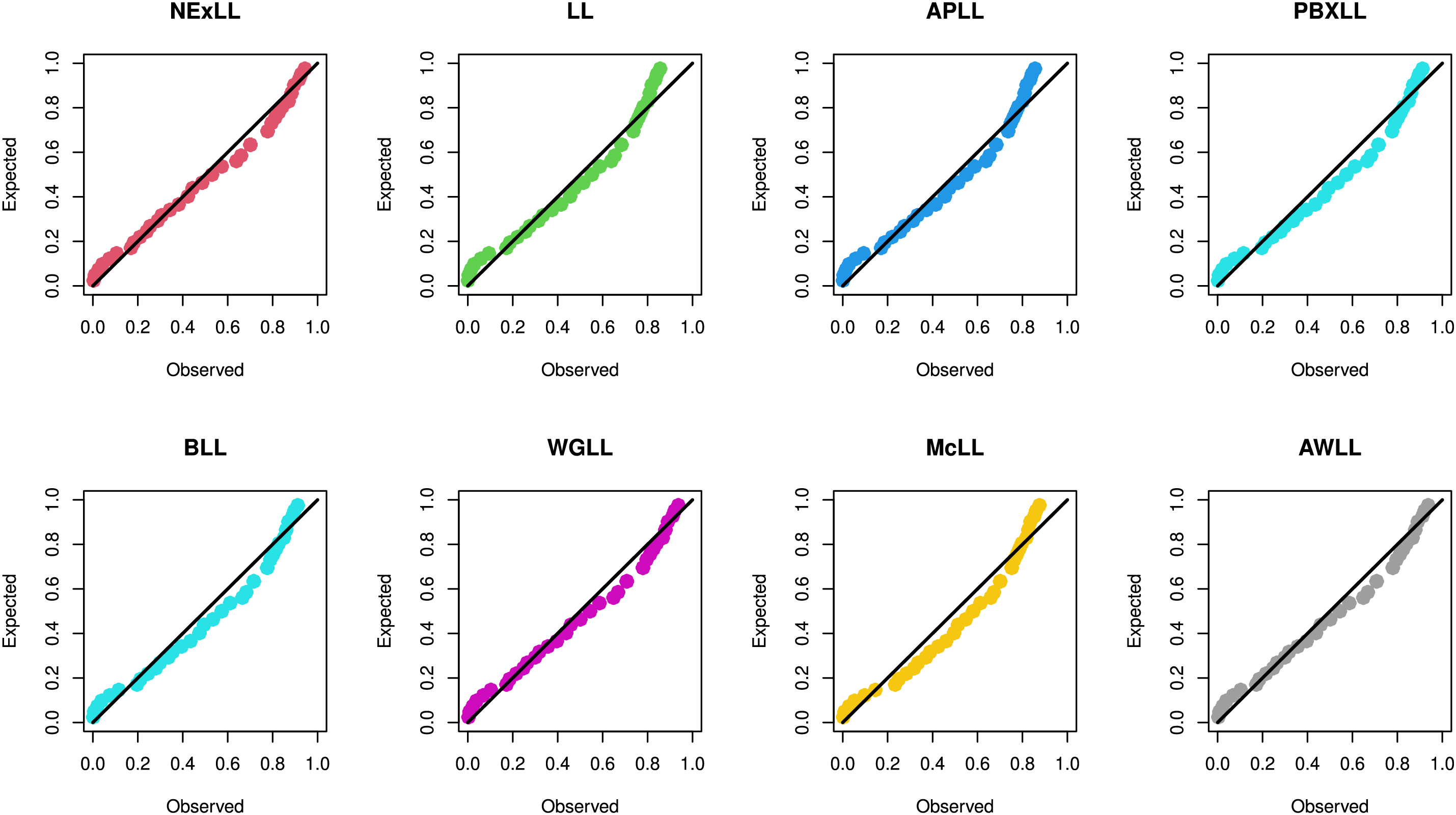
Figure 8: The PP plots of the fitted models for first dataset

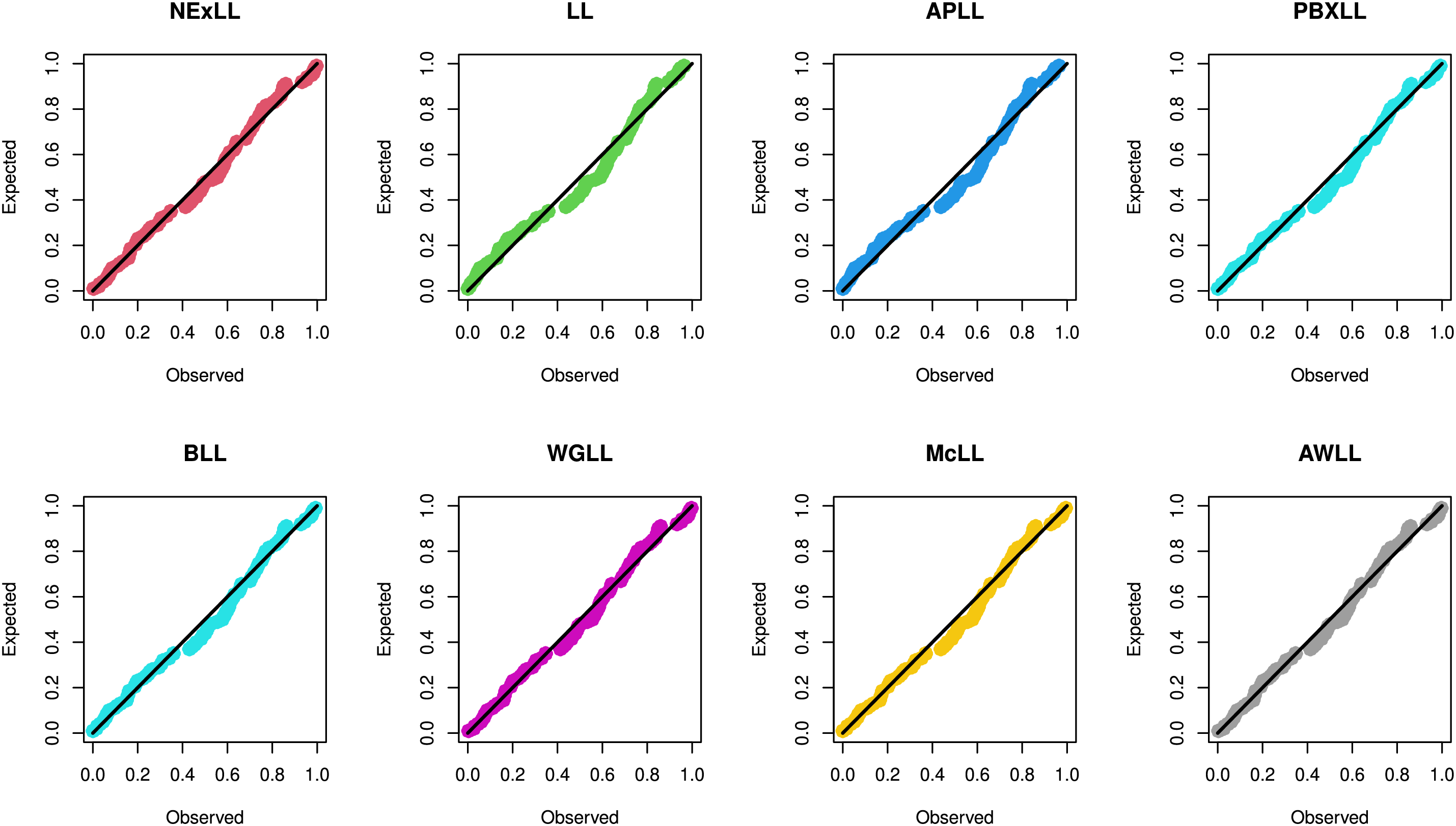
Figure 9: The PP plots of the fitted models for second dataset

7  Conclusions

In this study, we proposed a novel and flexible three-parameter distribution, called the NExLL distribution, as an extension of the classical log-logistic model. Unlike general NEx-H models, the NExLL distribution provides a fully closed-form, interpretable, and practically useful framework that can be directly applied to real-world survival and reliability data without requiring numerical approximation of its core functions. The proposed model exhibits remarkable flexibility, with a hazard rate function capable of capturing both monotonic and non-monotonic behaviors, and a density function that accommodates symmetric and asymmetric shapes—making it suitable for diverse survival and reliability applications. We thoroughly examined the mathematical properties of the NExLL distribution, and estimated its parameters using seven distinct estimation techniques. A comprehensive simulation study was conducted to evaluate the performance of these methods, revealing that the maximum product of spacings approach consistently yields the most efficient and accurate parameter estimates.

To demonstrate the practical utility of the model, we applied the NExLL distribution to two real-world lifetime datasets from the fields of engineering and reliability. The empirical results, supported by goodness-of-fit statistics and graphical analysis, confirm the NExLL model’s superior fitting capability over competing Log-Logistic-based models. The findings presented in this work contribute to the ongoing advancement of parametric survival modeling by offering a versatile distribution that can be further explored within broader frameworks, including the incorporation of trigonometric-based structures and machine learning-enhanced estimation strategies. As such, this study aligns with the objectives of the current special issue by pushing the boundaries of traditional parametric survival models and opening pathways for future interdisciplinary applications. Despite its promising performance, the proposed NExLL model is limited to complete and uncensored datasets, and its estimation under censoring or covariate settings remains unexplored. Future work may extend this model to handle censored data or incorporate covariates through regression frameworks for broader applicability.

Acknowledgement: Not applicable.

Funding Statement: Princess Nourah bint Abdulrahman University Researchers Supporting Project number (PNURSP2025R735), Princess Nourah bint Abdulrahman University, Riyadh, Saudi Arabia.

Author Contributions: Conceptualization, Hadeel AlQadi, Fatimah M. Alghamdi, Hamada H. Hassan, Mohamed E. Mead and Ahmed Z. Afify; methodology, Hamada H. Hassan, Mohamed E. Mead and Ahmed Z. Afify; software, Ahmed Z. Afify; validation, Hadeel AlQadi, Fatimah M. Alghamdi and Mohamed E. Mead; resources, Hadeel AlQadi and Fatimah M. Alghamdi; data curation, Hamada H. Hassan and Mohamed E. Mead; writing—original draft preparation, Hadeel AlQadi and Ahmed Z. Afify; writing—review and editing, Hadeel AlQadi, Fatimah M. Alghamdi, Hamada H. Hassan, Mohamed E. Mead and Ahmed Z. Afify; visualization, Hadeel AlQadi, Fatimah M. Alghamdi, Hamada H. Hassan and Mohamed E. Mead. All authors reviewed the results and approved the final version of the manuscript.

Availability of Data and Materials: The authors confirm that the data supporting the findings of this study are available within the article.

Ethics Approval: This study does not involve any human participants, animals, or identifiable personal data. The analysis is based entirely on publicly available datasets and simulated data. Therefore, ethics approval and consent to participate were not required.

Conflicts of Interest: The authors declare no conflicts of interest to report regarding the present study.

References

1. Marshall AW, Olkin I. A new method for adding a parameter to a family of distributions with application to the exponential and Weibull families. Biometrika. 1997;84(3):641–52. doi:10.1093/biomet/84.3.641. [Google Scholar] [CrossRef]

2. Eugene N, Lee C, Famoye F. Beta-normal distribution and its applications. Commun Stat-Theory Methods. 2002;31(4):497–512. doi:10.1081/sta-120003130. [Google Scholar] [CrossRef]

3. Cordeiro GM, de Castro M. A new family of generalized distributions. J Stat Comput Simul. 2011;81(7):883–98. doi:10.1080/00949650903530745. [Google Scholar] [CrossRef]

4. Alexander C, Cordeiro GM, Ortega EM, Sarabia JM. Generalized beta-generated distributions. Comput Stat Data Anal. 2012;56:1880–97. [Google Scholar]

5. Bourguignon M, Silva RB, Cordeiro GM. The Weibull-G family of probability distributions. J Data Sci. 2014;12:53–68. [Google Scholar]

6. Alizadeh M, Tahir MH, Cordeiro GM, Mansoor M, Zubair M, Hamedani G. The Kumaraswamy Marshal-Olkin family of distributions. J Egypt Math Soc. 2015;23(3):546–57. doi:10.1016/j.joems.2014.12.002. [Google Scholar] [CrossRef]

7. Hussain S, Rashid MS, Ul Hassan M, Ahmed R. The generalized alpha exponent power family of distributions: properties and applications. Mathematics. 2022;10(9):1421. doi:10.3390/math10091421. [Google Scholar] [CrossRef]

8. Hassan AS, Alsadat N, Chesneau C, Shawki AW. A novel weighted family of probability distributions with applications to world natural gas, oil, and gold reserves. Electron Res Archive. 2023;31(11). doi:10.3934/mbe.2023880. [Google Scholar] [PubMed] [CrossRef]

9. Okutu JK, Frempong NK, Appiah SK, Adebanji AO. A new generated family of distributions: statistical properties and applications with real-life data. Comput Math Methods. 2023;2023(1):9325679. doi:10.1155/2023/9325679. [Google Scholar] [CrossRef]

10. Al Abbasi JN, Afify AZ, Alnssyan B, Shama MS. The Lambert-G family: properties, inference, and applications. Comput Model Eng Sci. 2024;140:513–36. doi:10.32604/cmes.2024.046533. [Google Scholar] [CrossRef]

11. Jamal F, Alqawba M, Altayab Y, Iqbal T, Afify AZ. A unified exponential-H family for modeling real-life data: properties and inference. Heliyon. 2024;10(6):1–21. doi:10.1016/j.heliyon.2024.e27661. [Google Scholar] [PubMed] [CrossRef]

12. Fisk PR. The graduation of income distributions. Econometrica: J Econometric Soci. 1961;29:171–85. [Google Scholar]

13. Dagum C. A model of income distribution and the conditions of existence of moments of finite order. Bulletin Intl Stat Inst. 1975;46:199–205. [Google Scholar]

14. Shoukri MM, Mian IUH, Tracy DS. Sampling properties of estimators of the log-logistic distribution with application to Canadian precipitation data. Canadian J Stat. 1988;16(3):223–36. doi:10.2307/3314729. [Google Scholar] [CrossRef]

15. Arnold BC. Pareto distributions. Fairland, MD, USA: International Co-Operative Publication House; 1983. [Google Scholar]

16. Burr IW. Cumulative frequency functions. Annals Math Stat. 1942;13:215–32. [Google Scholar]

17. Mielke PW, Johnson ES. Three-parameter kappa distribution maximum likelihood estimates and likelihood ratio tests. Monthly Weather Rev. 1973;101:701–9. [Google Scholar]

18. Kleiber C, Kotz S. Statistical size distributions in economics and actuarial sciences. Hoboken, NJ, USA: John Wiley & Sons; 2003. [Google Scholar]

19. Nadar SS, Upadhyay V, Joshi S. Detecting clinical risk shift through log-logistic hazard change-point model. Mathematics. 2025;13(9):1457. doi:10.3390/math13091457. [Google Scholar] [CrossRef]

20. Felipe A, Jaenada M, Miranda P, Pardo L. Robust tests for log-logistic models based on minimum density power divergence estimators. arXiv:2503.14447. 2025. [Google Scholar]

21. Lemonte AJ. The beta log-logistic distribution. Brazilian J Probability Stat. 2014;28(3):313–32. doi:10.1214/12-bjps209. [Google Scholar] [CrossRef]

22. Gui W. Marshall–Olkin extended log-logistic distribution and its application in minification processes. Appl Math Sci. 2013;7:3947–61. doi:10.12988/ams.2013.35268. [Google Scholar] [CrossRef]

23. Tahir MH, Mansoor M, Zubair M, Hamedani GG. McDonald log-logistic distribution with an application to breast cancer data. J Stat Theory Appl. 2014;13:65–82. [Google Scholar]

24. Ramos MWA, Cordeiro GM, Marinho PRD, Dias CRB, Hamedani GG. The Zografos-Balakrishnan log-logistic distribution: properties and applications. J Stat Theory Appl. 2013;12:225–44. [Google Scholar]

25. Cakmakyapan S, Ozel G, Gebaly YMHE, Hamedani GG. The Kumaraswamy Marshall-Olkin log-logistic distribution with application. J Stat Theory and Appl. 2018;17:59–76. [Google Scholar]

26. Almamy JA. Extended Poisson log-logistic distribution. Int J Stat Probab. 2019;8:56–69. [Google Scholar]

27. Cordeiro GM, Afify AZ, Ortega EM, Suzuki AK, Mead ME. The odd Lomax generator of distributions: properties, estimation and applications. J Comput Appl Math. 2019;347:222–37. doi:10.1016/j.cam.2018.08.008. [Google Scholar] [CrossRef]

28. Aldahlan MA. Alpha power transformed log-logistic distribution with application to breaking stress data. Adv Math Phy. 2020;2020(3):1–9. doi:10.1155/2020/2193787. [Google Scholar] [CrossRef]

29. Alfaer NM, Gemeay AM, Aljohani HM, Afify AZ. The extended log-logistic distribution: inference and actuarial applications. Mathematics. 2021;9(12):1386. doi:10.3390/math9121386. [Google Scholar] [CrossRef]

30. Gaire AK, Gurung YB. Skew log-logistic distribution: properties and application. Stat Transition New Ser. 2024;25:43–62. [Google Scholar]

31. Rahman MM, Darwish JA, Shahbaz SH, Hamedani G, Shahbaz MQ. A new cubic transmuted log-logistic distribution: properties, applications, and characterizations. Adv Appl Stat. 2024;91(3):335–61. doi:10.17654/0972361724018. [Google Scholar] [CrossRef]

32. Panitanarak U, Ishaq AI, Abiodun AA, Daud H, Suleiman AA. A new Maxwell-log logistic distribution and its applications for mortality rate data. J Nigerian Soc Phys Sci. 2025;7:1976–6. doi:10.46481/jnsps.2025.1976. [Google Scholar] [CrossRef]

33. Ahmed AD, Yassin YT, Wahhab BIA, Abdullah EKA. Comparison of some methods for estimating the parameters of the type–II generalized log logistic distribution using simulation. Iraqi Statisticians J. 2025;2:344–50. [Google Scholar]

34. Afify AZ, Abdelall YY, AlQadi H, Mahran HA. The modified log-logistic distribution: properties and inference with real-life data applications. Contemporary Math. 2025;862–902. doi:10.37256/cm.6120256273. [Google Scholar] [CrossRef]

35. Lorenz MO. Methods of measuring the concentration of wealth. Publications Am Stat Assoc. 1905;9(70):209–19. doi:10.1080/15225437.1905.10503443. [Google Scholar] [CrossRef]

36. Arcagni A, Porro F. The graphical representation of the inequality. Dipartimento Di Statistica E Metodi Quantitativi Working Papers. 2014;37:419–37. [Google Scholar]

37. Cheng RCH, Amin NAK. Estimating parameters in continuous univariate distributions with a shifted origin. J Royal Stat Soc Ser B (Methodol). 1983;45(3):394–403. doi:10.1111/j.2517-6161.1983.tb01268.x. [Google Scholar] [CrossRef]

38. Cheng RCH, Amin NAK. Maximum product-of-spacings estimation with applications to the lognormal distribution. In: Math report. Cardiff: University of Wales Institute of Science and Technology; 1979. [Google Scholar]

39. Xu K, Xie M, Tang LC, Ho SL. Application of neural networks in forecasting engine systems reliability. Appl Soft Comput. 2003;2(4):255–68. doi:10.1016/s1568-4946(02)00059-5. [Google Scholar] [CrossRef]

40. Nichols MD, Padgett WJ. A bootstrap control chart for Weibull percentiles. Qual Reliab Eng Intl. 2006;22(2):141–51. doi:10.1002/qre.691. [Google Scholar] [CrossRef]

41. Shehata W, Abdullah MM, Refaie MK. A novel four-parameter log-logistic model: mathematical properties and applications to breaking stress, survival times and leukemia data. Pakistan J Stat Oper Res. 2022;18:133–49. doi:10.18187/pjsor.v18i1.3268. [Google Scholar] [CrossRef]

42. Hemeda S. Additive Weibull log logistic distribution: properties and application. J Adv Res Appl Math Stat. 2018;3:8–15. [Google Scholar]