Meyer Wavelet Transform and Jaccard Deep Q Net for Small Object Classification Using Multi-Modal Images

1  Introduction

Object detection is crucial in fields like autonomous piloting and medical diagnosis but often relies on single modalities like Red green and blue (RGB) or Infrared (IR) imaging, which lack sufficient complementary information [1,2]. Advances in remote sensing imagery (RSI) have improved detection accuracy through multimodal integration, particularly combining RGB and IR [3,4]. While effective, these techniques are complex and challenging to apply in resource-limited environments, especially when processing large datasets from drones and satellites [5]. Small object detection plays a vital role in critical applications such as military surveillance, disaster response, and autonomous navigation. Another important area is medical imaging. In fields like oncology and neurology, detecting small lesions, tumors, or abnormalities at an early stage is essential for timely diagnosis and effective treatment [6,7]. Frameworks such as Vision Deep-AI demonstrate the growing demand for advanced detection solutions [8,9]. Infrared Small Object Segmentation (ISOS) faces unique challenges due to the small size, low visibility, and sparse distribution of objects in IR images [10]. These factors create a significant imbalance between objects and their background, complicating detection and localization. Effective segmentation is critical to minimize missed detections (MD) and false alarms (FA). Advanced techniques use machine learning to extract features, classify objects, and ensure precise localization and measurement [11]. Similarly, Deep learning (DL) is widely used for object localization and classification, offering superior performance when sufficient training data and computational resources are available [12–16]. Techniques like Convolutional Neural Networks (CNN) and Region-based CNN (R-CNN) utilize selective search algorithms to identify regions, extract features, and classify objects, though R-CNN has limitations in processing speed and scalability [17–20]. Advancements such as Spatial Pyramid Pooling (SPP) and Fast R-CNN address these issues by improving speed and integrating object localization and classification in a streamlined process [21]. Feature Pyramid Networks (FPN) further enhance detection by generating high-quality feature maps for classification and bounding tasks [22,23]. Additionally, novel approaches like wavelet-based encoder-decoder networks combine cross-modal attention and frequency-domain transforms for advanced video segmentation, supported by large-scale datasets [24,25].

1.1 Motivation

In recent years, rapid advancements in remote sensing technologies have enabled the acquisition of high-dimensional and diverse image data from various platforms, including satellites, drones, and airborne sensors. However, traditional small object detection methods continue to face several critical challenges, which are given as follows:

•   Small objects typically occupy only a few pixels, making them difficult to distinguish from background noise and clutter.

•   In the traditional methods, the low spatial resolution, occlusion, poor contrast, and sparse object distribution factors further complicate the detection process across various image modalities.

•   Most existing object detection techniques rely on single-modal data, limiting their ability to accurately detect small objects in complex and cluttered environments.

These limitations in conventional approaches highlight the need for more effective and robust detection methods. Consequently, these challenges serve as the primary motivation for developing a novel small object classification model.

1.2 Research Objectives

The objectives of this research are mentioned as follows:

•   To develop a novel small object detection framework that combines complementary information from multiple remote sensing modalities.

•   To design an enhanced detection architecture, named JDQN by integrating the Jaccard similarity measure with DQN through regression modeling for improved object localization and classification.

•   To employ a DMN to perform effective fusion of detection outputs from multiple modalities, thereby improving accuracy and reducing errors.

The key intent of this work is to devise a DL network for detecting small objects using RSI. In this method, the multimodal images are subject to various processes, such as preprocessing, image transformation, segmentation, feature extraction, detection, and fusion. The input images are fed to an Adaptive Kalman Filter (AKF) for denoising the image. Later, the image is transformed into the frequency domain from the spatial domain using the Meyer Wavelet Transform (MWT), and then the small objects in the image are segmented with the help of the Deepjoint segmentation. Afterward, the most noticeable features in the image are excerpted and then applied to the JDQN, which is formulated by incorporating the Jaccard similarity measure with DQN. Then, the obtained results are fused using the DMN to obtain the final detected output.

The significant contribution of this research is as follows:

•   Proposed JDQN for small object detection: Small object detection is performed in this study using the JDQN, which integrates the Jaccard similarity measure into DQN using regression analysis. Further, the detected outputs obtained from the various modalities are fused using the DMN.

The structure of this paper is outlined as follows: Section 2 provides an overview of recent advancements in small object detection, Section 3 introduces the proposed JDQN approach, Section 4 presents the results along with their analysis, and Section 5 concludes the study.

2  Related Work

Object detection is fundamental to many applications, but detecting small objects in remote sensing (RS) remains challenging due to their minimal size often reduced to a single pixel, and the scarcity of datasets caused by the difficulty of acquiring RS images. This segment reviews deep learning (DL)-based frameworks from the literature that inspired the development of the JDQN.

2.1 Literature Review

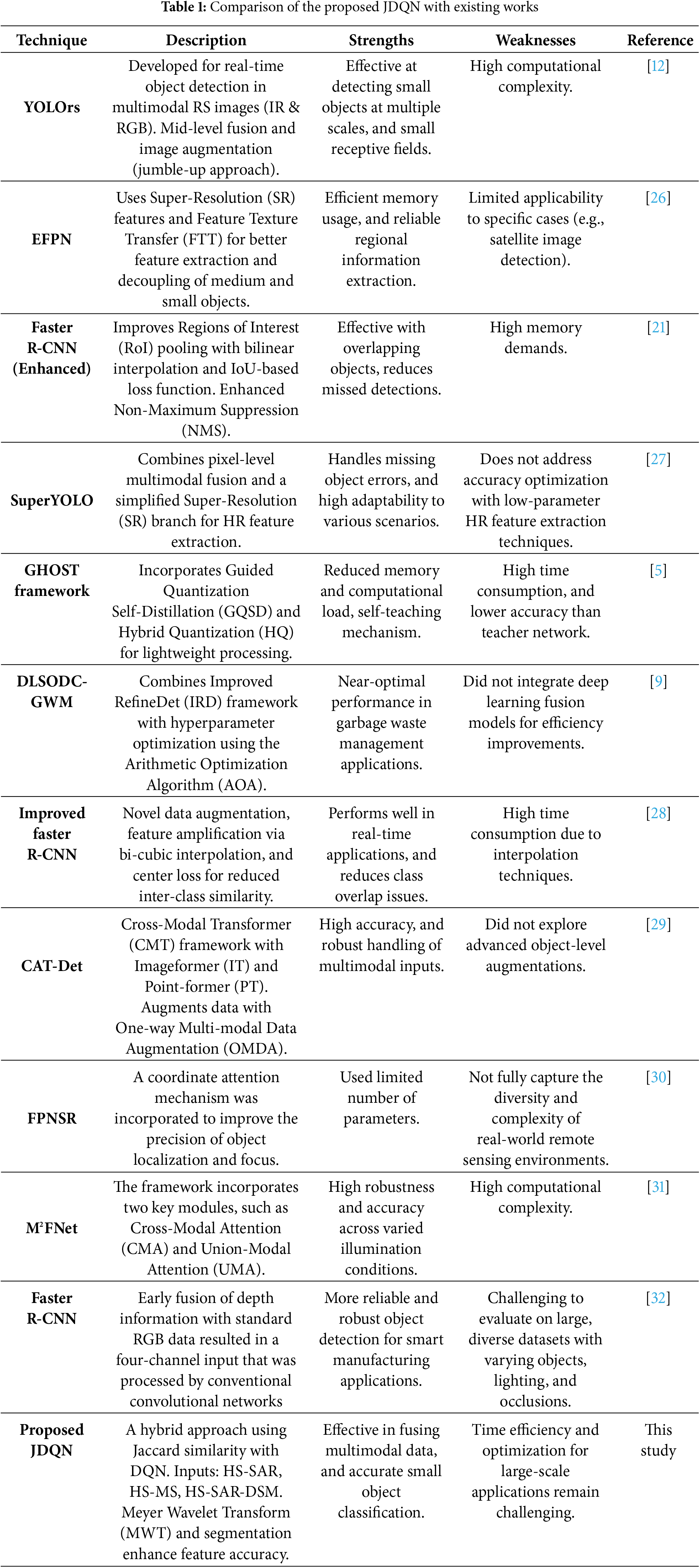
Several advanced frameworks have been developed for small object detection in remote sensing (RS) applications. The YOLOrs model [12] utilizes IR and RGB modalities along with a mid-level fusion framework for real-time detection, achieving multi-scale object detection with small receptive fields; however, this comes at a high computational cost. The Extended Feature Pyramid Network (EFPN) [26], enhances detection using Super-Resolution (SR) features and a Feature Texture Transfer (FTT) module, efficiently handling medium and small object detection while addressing the background-foreground imbalance. However, it lacks the integration of additional detectors for robustness. Faster region-based NN (Faster R-CNN) [21] improves object localization and bounding box regression through enhanced RoI pooling, multi-scale feature fusion, and Non-Maximum Suppression (NMS), reducing detection errors but demanding significant computational resources. In [27], SuperYOLO employs pixel-level multimodal fusion and a simplified SR branch to retain high-resolution features, effectively reducing detection errors while maintaining flexibility. However, it does not optimize accuracy through low-parameter models for feature extraction. Each approach demonstrates strengths and limitations, advancing small object detection in RS.

Several innovative approaches have been proposed for small object detection in various domains. The GHOST framework [5] introduced Guided Hybrid Quantization with One-to-one Self-Teaching (OST), leveraging Guided Quantization Self-Distillation (GQSD) to enable self-learning without external supervision, achieving reduced memory and computational demands but suffering from high time consumption. The DLSODC-GWM model [9] applied Improved Refine Det (IRD) for waste object detection and classification, optimizing hyperparameters using the Arithmetic Optimization Algorithm (AOA) and Functional Link Neural Network (FLNN) for classification, but lacked the integration of DL fusion models for enhanced efficiency. An Improved Faster R-CNN [28] was developed for industrial defect detection, addressing data imbalance with novel oversampling and stitching augmentation techniques and reducing inter-class similarity with center loss, though interpolation increased time consumption. The CAT-Det framework [29] employed a Cross-Modal Transformer (CMT) with Image-former (IT) and Point-former (PT) branches for multimodal 3D object detection, augmented by the One-way Multi-modal Data Augmentation (OMDA) method, achieving high accuracy but lacking object-level augmentations for further enhancement. Table 1 highlights the key differences and similarities between our work and previous studies, providing a clearer context for our contributions. The Feature Pyramid Network for Super Resolution (FPNSR) [30] was developed to enhance the detection of small objects. In this framework, a coordinate attention mechanism was incorporated to improve the precision of object localization and focus. The model was designed with a limited number of parameters, making it suitable for deployment on resource-constrained devices. However, the evaluation was conducted on a relatively small dataset, which may not fully capture the diversity and complexity of real-world remote sensing environments. Additionally, the Multi-Modal Fusion Network (M2FNet) [31], based on the Transformer architecture, was developed for object detection using multimodal data. The framework incorporates two key modules, such as Cross-Modal Attention (CMA) and Union-Modal Attention (UMA). While M2FNet demonstrates high robustness and accuracy across varied illumination conditions, its major limitation lies in the increased computational complexity introduced by the Transformer-based design. The Faster R-CNN [32] model was implemented for object detection using camera images, where early fusion of depth information with standard RGB data resulted in a four-channel input that was processed by conventional convolutional networks. This approach enabled more reliable and robust object detection for smart manufacturing applications. However, it was difficult to evaluate the model on larger datasets featuring diverse object configurations, lighting conditions, and occlusion scenarios.

2.2 Research Gaps of the Existing Methods

The difficulties encountered while reviewing the available strategies for small object classification are deliberated below.

•   The key issue with YOLOrs [12] in object detection is that, while the technique is efficient at retrieving rich semantic information with limited tuning, the performance is affected by the confidence levels. A high confidence value results in false negatives, while a low value leads to the detection of undesired backgrounds.

•   The EFPN technique designed in [26] performs well and effectively identifies medium and small objects. However, it struggles to adapt to specific small object detection scenarios, such as satellite image detection or face detection.

•   In Faster R-CNN [21], the method offers superior results even in cases of overlapping objects. However, it requires high memory resources.

•   The GHOST framework [5] is lightweight and demonstrates superior information retention capabilities. However, its accuracy is lower.

3  Proposed JDQN for Small Object Classification

Small object classification poses significant challenges due to limited information and low resolution, and applying the same object detection techniques across different environments is also challenging. This section expounds on the hybrid deep learning network named JDQN proposed in this study for classifying small objects. In this research, small object classification is carried out using three types of images, such as HS-SAR, HS-MS, and HS-SAR-DSM. The input images in the three modalities are subject simultaneously to pre-processing phase at first, where the Adaptive Kalman Filter (AKF) [33] is used to denoise the image thereby enhancing the image quality. After that, the pre-processed image is fed to the image transformation, where the denoised image is subject to Meyer Wavelet Transform (MWT) [34] to convert the image from the spatial domain to the frequency domain. Thereafter, segmentation of the small objects from the background region is accomplished using Deepjoint segmentation [35]. Further, various features, like oriented FAST and rotated BRIEF (ORB) [36], Local vector pattern (LVP) [37], and statistical features like mean, variance, standard deviation, kurtosis, and skewness are excerpted from the segmented image. Afterward, small object classification is performed by the proposed JDQN, which is developed by the incorporation of the Jaccard index [38] and Deep Q-Net [39].

Finally, the three resultant outputs are combined using the DMN [40] to get the final classified output. The various processes involved in small object classification using the proposed JDQN are depicted in Fig. 1. The flowchart of the proposed model is provided in Fig. 2.

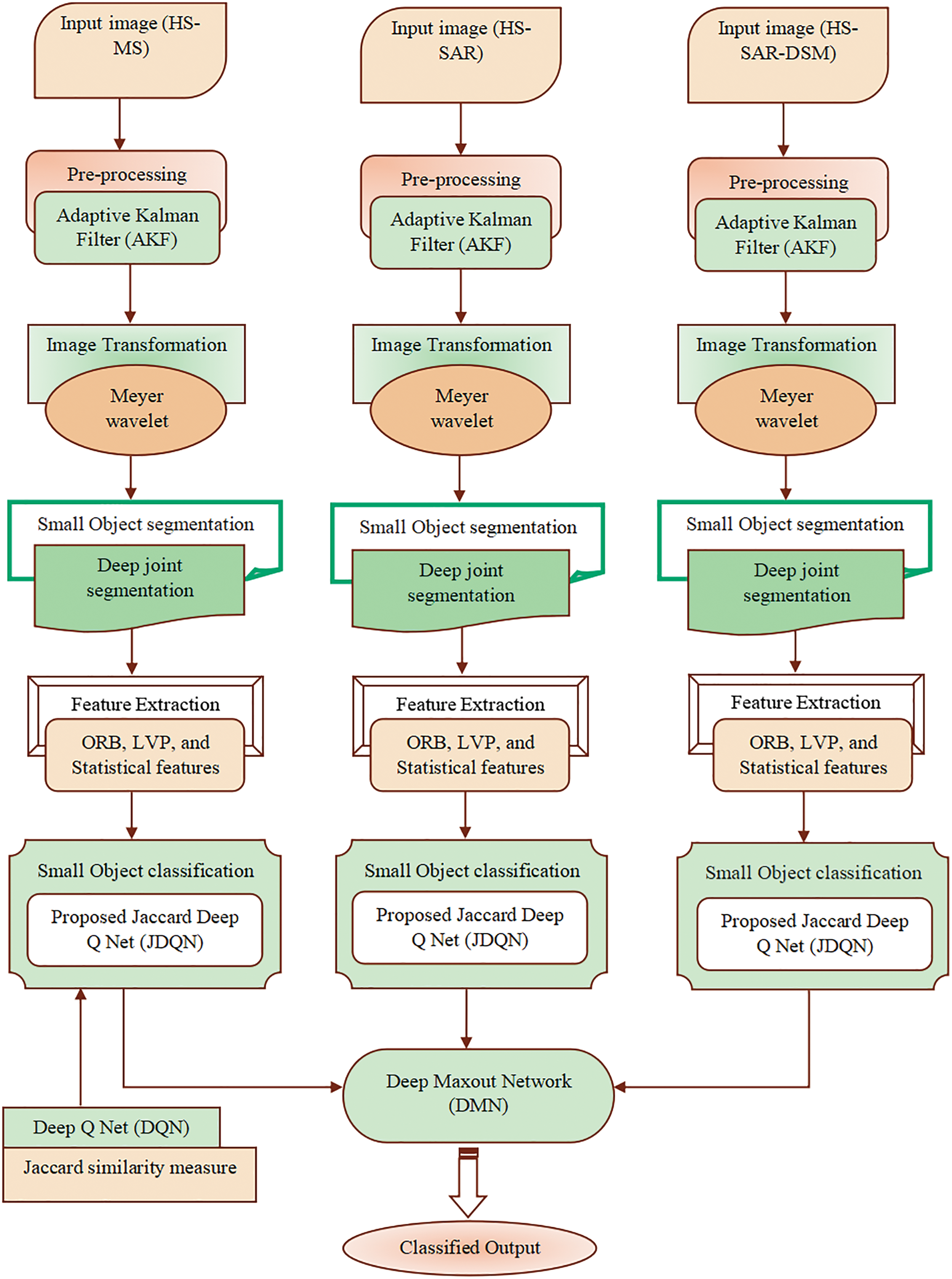
Figure 1: Block diagram for small object classification using the proposed JDQN

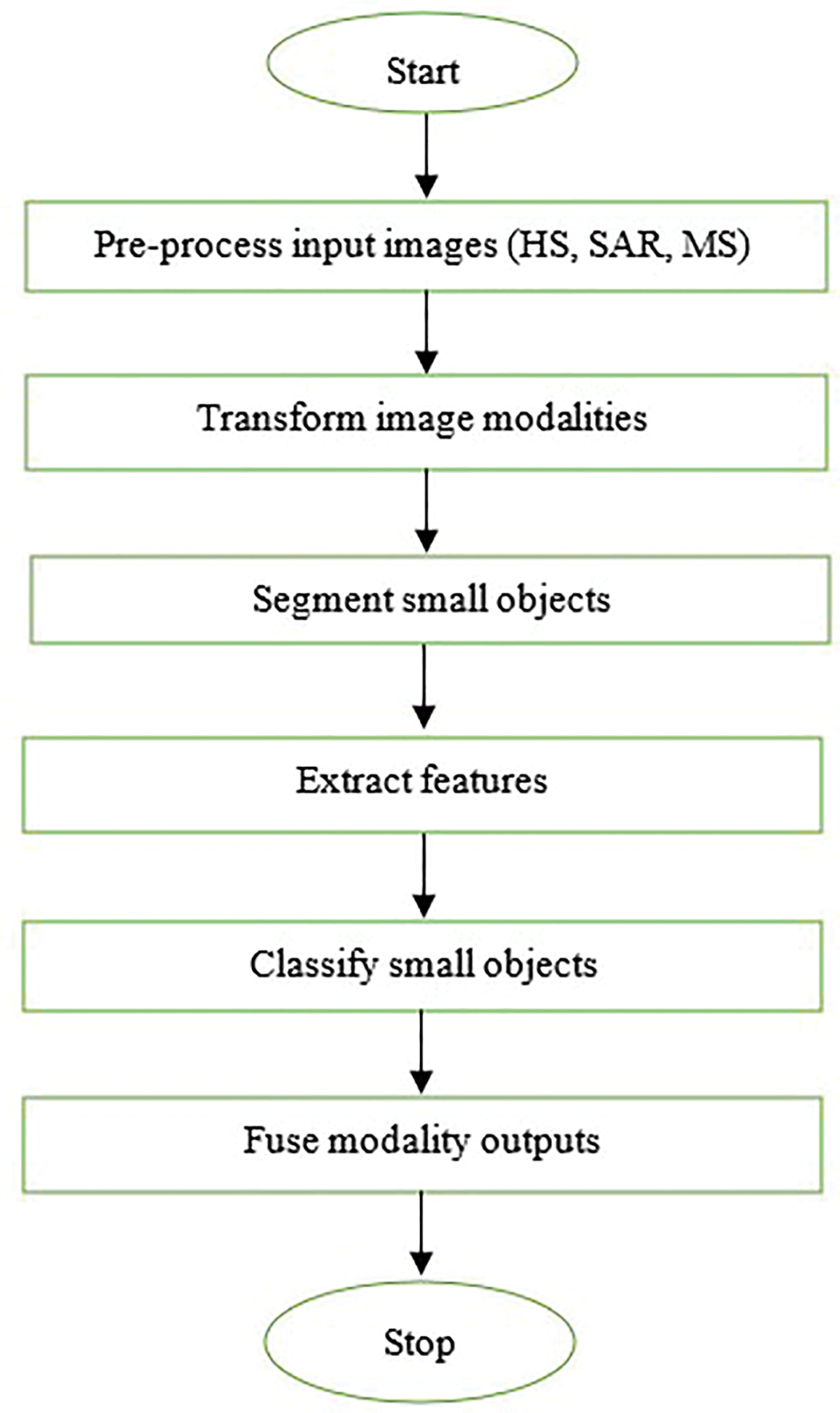
Figure 2: Flowchart of the proposed JDQN

3.1 Data Acquisition

The input images used for small object classification using the proposed JDQN are assimilated from a dataset A encompassing a total of n images, which is formulated as given follows in Eq. (1):

A={A1,A2,…,Aj,…,An}(1)

wherein, Aj infers the jth image in the database and it is considered for small object classification.

3.2 Pre-Processing

The primary step in object classification is to pre-process the image using the AKF [33]. This is an essential task as noise in the images can degrade the classification ability of the JDQN. Though the Kalman filter is highly effective in processing the data accurately, the output attained is highly dependent on the previous information about the noise as well as the mathematical model. Hence, to overcome these issues, the AKF is used, which estimates and corrects uncertain and unknown noise and model parameters continuously during filtering. AKF is highly robust and produces filtered values that are near the true values. The following equation Eq. (2) is used to find the output of AKF.

L^i=(BiTS¯iBi+αiSL¯i)−1(BiTS¯iai+αiSL¯iL¯i)(2)

where, L^i characterizes the output response of the AKF, αi refers to the adaptive factor, B¯i represents the equivalent weight matrix of output Si at time instance ti, and SL¯i=ΣL¯i−1 signifies the weighted matrix of the estimated state vector Li. The noise-removed image thus obtained using the AKF is characterized as C, and is applied to the image transformation phase.

3.3 Image Transformation

The denoised image C is applied to MWT [34] for converting the image from the spatial domain to the frequency domain. Meyers wavelet is mainly used here owing to its finite spectrum, fast attenuation, and smoothness. It was devised for smoothing the sinc scaling function and is defined as a function of ν. The Meyer wavelet is a continuous orthogonal wavelet and is infinitely differentiable. A single-level decomposition (Level 1) is applied to retain the dominant signal characteristics while reducing redundancy. The boundary mode is set to ‘symmetric’, which helps to minimize edge effects and artificial distortions during transformation, preserving the signal continuity. The sampling rate is fixed at 100 Hz, which is sufficient to capture relevant frequency components without unnecessary data overhead. The following in Eqs. (3) & (4) defines the scaling function of the MWT.

ϕMWT(x)={12π;x<2π312πcos⁡(π2ν(3x2π−1));2π3<x<4π30;otherwise(3)

where,

ν(y)={0;y<0y;0≤y≤11;y>1(4)

Further, the wavelet spectrum is given by Eq. (5),

ψMWT(x)={12πsin⁡(π2ν(3|x|2π−1))ejx2;2π3<|x|<4π312πcos⁡(π2ν(3|x|2π−1))ejx2;4π3<|x|<8π30;otherwise(5)

The MWT transforms the denoised image C into multiple sub-bands. After the first level of decomposition, four sub-bands—High-High (HH), High-Low (HL), Low-High (LH), and Low-Low (LL)—are obtained. Among these four bands, the LL band is chosen for further processing. Consider the Meyer wavelet transformed output, represented as Z, and is subjected to segmentation.

3.4 Small Object Segmentation

The next process is to segment the object from the background using the wavelet-transformed output Z. Here, segmentation is accomplished by adopting the DeepJoint segmentation [35], which is an approach utilized to segment the region of interest based on similarities among the bi-constraints and regions, and the distance between the segmented and deep points. Here, the minimum distance function is employed to identify the deep points, and thereafter, the identification of the segmented points is accomplished, and then are iterative process is utilized to combine the grid segments.

Small object segmentation involves the following stages:

1.    Joining, region fusion, and segment point generation.

2.    Initially, the wavelet-transformed output Z is divided into multiple grids, and the pixels are merged based on the threshold and mean levels during the joining stage.

3.    Afterward, region fusion is performed considering the bi-constraints and resemblance of the regions. Grids with the minimal mean value are merged to generate the mapped points.

4.    Finally, the optimal segments are identified by calculating the distance between the segmented and deep points.

The following steps are used for segmenting small objects in the image. The iteration considered this segmentation is 100.

i) Grid creation: The primary process in segmenting the object from the background is to split the wavelet-transformed image Z into several grids, and it is expressed in Eq. (6),

H={H1,H2,…,Hh,…,Hχ}(6)

where, χ indicates the number of grids and Hh refers to the hth grid considered for processing.

ii) Joining: As soon as the grid is created, the pixels inside the grid are merged in the joining phase taking into account the threshold and mean values. Here, the average of the pixel values in the grid is measured to compute the mean and then, a constant threshold is used to process the mean for deciding whether a pixel has to be joined or not. In this work, a threshold value unity is considered, and the following in Eq. (7) is used to compute the mean.

Hh=∑l=1oElo(7)

Here, o specifies the count of pixels present in the hth grid, and El characterizes the pixel value linked with the hthgrid. The following Eq. (8) is used to combine the pixels.

Hh=∑l=1oElo±γ(8)

wherein, χ signifies the threshold, and here the threshold value considered is 0.65, which is selected after experimental tuning across different small object scenarios, and is found to balance over- and under-segmentation effectively.

iii) Region fusion: The regions are fused in this stage by considering the allotted grids for creating a region fusion matrix. Fusion is accomplished after the matrix generation considering the similarity between the bi-constraints and pixel intensity. The region fusion is accomplished only when both constraints are satisfied.

(1)   The mean value Dh should not exceed 3.

(2)   For each grid, a single grid point only has to be considered.

Using the two constraints above, the region similarity is determined and fusion of the regions is performed to identify the mapped points. The region similarity is depicted using Eq. (9),

Dh=∑i=1FEiϑG(9)

where, the pixels merged in the joining process are termed as Eiϑ and the count of fused pixels in the grid Hh is represented by G. The fusion of the grids yields the mapped points, represented as Eq. (10),

M={M1,M2,…,Mb,…,Mm}(10)

wherein, m signifies the count of mapped points in the wavelet-transformed image.

iv) Recognize deep points: The deep points are recognized by considering the mapped points and missed pixels in the joining stage. Pixels within the threshold boundary or left out during joining are considered missed pixels, as expressed in Eq. (11),

(I)={JM};1<M≤λ(11)

Here, JM signifies the missed pixel, missed pixel count is characterized as λ. The deep points are recognized by summing up the missed and mapped pixels as follows in Eq. (12),

λpoints=I+Mb(12)

v) Recognize the best segments: An iterative process is carried out on the deep points to determine the optimal segments. Initially, the selection of the segmented points Y is carried out arbitrarily, and three segmented points are chosen from the α deep points. Thereafter, the distance from the deep points to the segmented points is measured and the new segmented point is identified by locating the points with the shortest distance. The distance is measured as follows in Eq. (13),

δ=∑j=1α(Yb−λpoints)2(13)

vi) Termination: The phases are repeated until the finest segment points are attained.

In the above manner, the object region is segmented using the DeepJoint segmentation and the resultant output is signified as P.

3.5 Feature Extraction

The segmented image B is then subject to the feature extraction phase, wherein various textual features, like ORB [36], and LVP [37] are first extracted. Thereafter, statistical features [41], namely mean, variance, Standard Deviation (SD), skewness and kurtosis are found from textual features. This process is carried out for all the small objects in the image.

i) LVP

LVP is generally utilized for reducing the feature length by minimizing the redundant information in the segmented image B, and is an enhanced Local Tetra Pattern (LTrP). The LVP feature is computed based on the following Eq. (14),

Q1=LVPd,e(Tc)={LVPd,e,λ(Tc)|λ=0∘,45∘,90∘,135∘}(14)

where, Q1 depicts the LVP features, Tc denotes the target pixel, d signifies the number of neighboring pixels of Tc in the radius e, and λ designates the index angle associated with the variation in the orientation, and LVPd,e,λ(Tc) is formulated as follows in Eq. (15),

LVPd,e,λ(Tc)=f5(ℜλ,δ(T1,e),ℜλ+45∘,δ(T1,e),ℜλ,δ(Tc),ℜλ+45∘,δ(Tc)),f5(ℜλ,δ(T2,e),ℜλ+45∘,δ(T2,e),ℜλ,δ(Tc),ℜλ+45∘,δ(Tc)),…,f5(ℜλ,δ(Tγ,e),ℜλ+45∘,δ(Tγ,e),ℜλ,δ(Tc),ℜλ+45∘,δ(Tc))|γ=1,2,..,d,e=1|(15)

where, f5(⋅) represents the transformation ratio, δ indicates the distance to the adjacent pixel from Tc, ℜλ,δ specifies the directional vector.

ii) ORB

ORB [36] is a feature extraction approach that was created as an OpenCV and the features determined using are less sensitive to noise and produce superior results. The patch moment is used to compute the centroid of the segmented image B as given in Eq. (16),

crs=∑x,yxrysϑ(x,y)(16)

Here, ϑ(x,y) refers to the intensity of the patch, and crs specifies the moment of the patch. The corner orientation is measured by utilizing the intensity centroid of the image patch and is expressed as in Eq. (17),

O=(c10c00,c01c00)(17)

Further, the angle from the image patches to centroid is formulated in Eq. (18),

atan⁡2(c10c00,c01c00)=atan⁡2(c01,c10)(18)

where, atan⁡2 characterizes the quadrant-aware arctan. The ORB feature thus determined is symbolized as Q2.

The ORB and LVP features that are determined are merged to produce a textual feature image, which is expressed in Eq. (19),

QT={Q1,Q2}(19)

where Q1 signifies the LVP feature and Q2 depicts the ORB feature.

iii) Statistical features

After determining the textual image feature QT, the statistical features [41], such as mean, variance, standard deviation, kurtosis and skewness are measured.

a) Mean

This feature is utilized for gauging the data concentration in the textual feature image Q and is expressed in Eq. (20),

Q3=∑j=0χ−1j∗ξ(j)(20)

where, Q3 represents the mean feature, χ signifies the overall gray count, and ξ(j) symbolizes the likelihood of the occurrence of the pixel with gray value j in the image TQ.

b) Variance

This refers to the difference in the intensity of a pixel from the average value and is formulated in Eq. (21),

Q4=∑j=0χ−1(j−Q3)2∗ξ(j)(21)

wherein, Q4 designates the variance parameter.

c) SD

The distribution of data around the average value is known as SD, and is determined by considering the square root of the variance, and is given in Eq. (22),

Q5=Q4=∑j=0χ−1(j−Q3)2∗ξ(j)(22)

wherein, Q5 signifies the SD.

d) Kurtosis

The tiredness of the distribution by the normal distribution is known as kurtosis, and it is referred to as the “fourth normalized moment” also, and is measured by utilizing the following in Eq. (23),

Q6=Q3−4∑j=0χ−1(j−Q3)4∗ξ(j)(23)

where, Q6 designates the kurtosis parameter.

e) Skewness

Skewness is known as the degree of asymmetry of a specific feature about the mean value and is formulated as follows in Eq. (24),

Q7=Q3−3∑j=0χ−1(j−Q3)3∗ξ(j)(24)

wherein, skewness is symbolized as Q7.

The statistical features determined are concatenated to yield the feature vector, and are specified in Eq. (25),

QS={Q3,Q4,Q5,Q6,Q7}(25)

where, Q3 designates the mean feature, Q4 terms variance, Q5 is SD, Q6 designates kurtosis, and Q7 is the skewness feature. The feature vector QS is applied to the JDQN for detecting the small objects.

3.6 Small Object Classification Using Proposed JDQN

The feature vector QS is then applied to the JDQN for detecting the small objects, where the JDQN is formulated by the Jaccard similarity measure [38] with the DQN [39] using regression analysis. Here, the JDQN encompasses three components: the DQN model, the Jaccard layer, and the Jaccard Fused DQN (JFDQN) model. The JDQN performs small object detection based on the input image Aj, the feature vector QS, and the textual feature image QT. Initially, the input image Aj is applied to the DQN, which produces a detected output U1. However, this output doesn’t represent the detection of the objects at a fine level.

To overcome this limitation, the Jaccard similarity measure [38] is incorporated into the DQN using regression analysis to yield a finer result. The output U1 generated by the DQN and the statistical feature set QS is applied to the Jaccard layer, where the Jaccard similarity is used to find the likeness between the feature vectors. The output generated is characterized as U2. Thereafter, the output U2, feature vector QS, and textual feature image QT are subject to the JFDQN layer to produce the final output U3. Here, all the inputs are combined using regression analysis and this is carried out using the Fractional Calculus (FC) [42]. The architectural view of the JDQN is exemplified in Fig. 3.

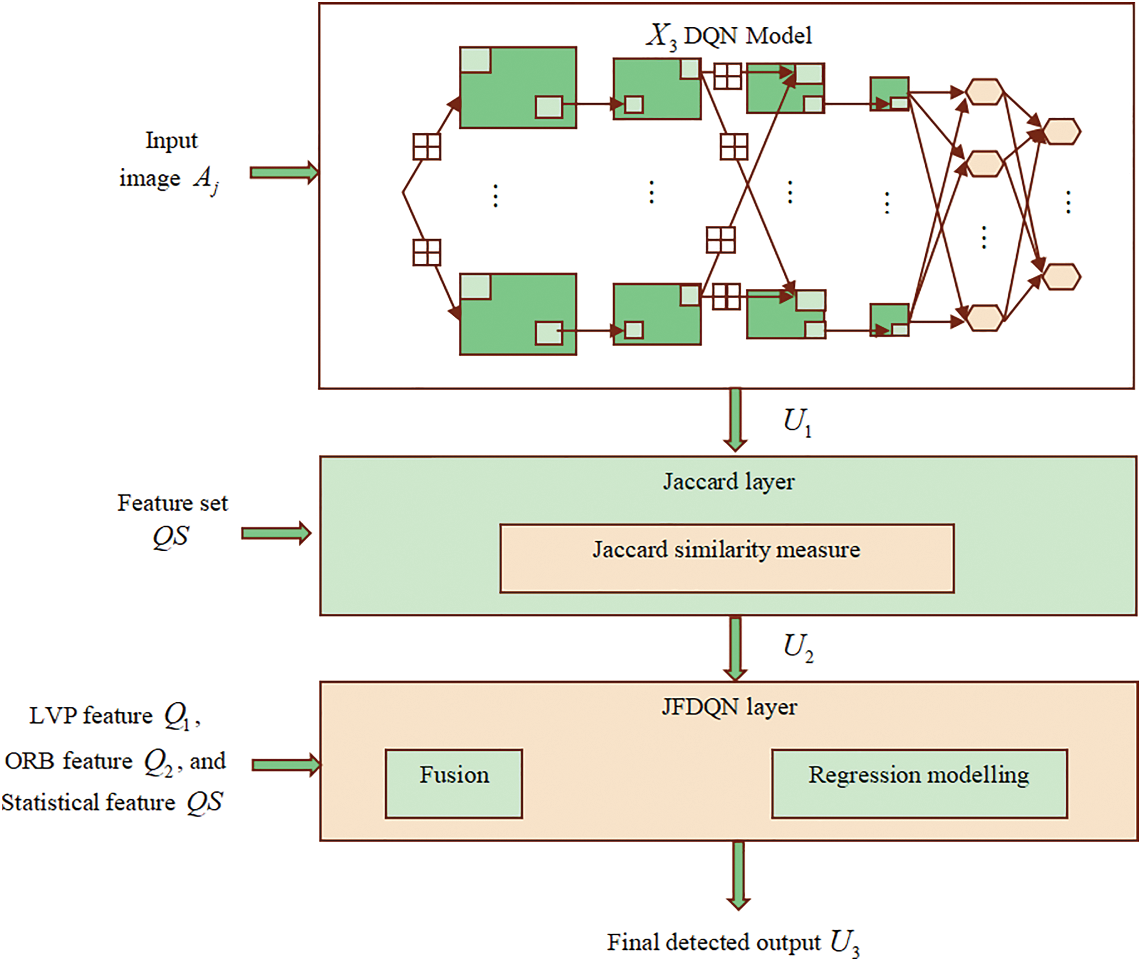
Figure 3: Structural view of the JDQN

3.6.1 DQN

The Deep Q-Network (DQN) [39,43] is a deep learning model that integrates Q-learning, a popular reinforcement learning (RL) approach, with deep neural networks (DNN) to estimate the Q-function’s action values. The anticipated discounted cumulative reward yields the active function value and is represented in Eq. (26),

Vtπ(ut,wt)=E[∑i=0∞βiρt+i|ut=u,wt=wπ](26)

where ut refers to the state observation, wt depicts the action, β characterizes the discount factor, and ρ is the reward. The ideal value of the action function is represented as V∗(u,w)=maxπVπ(u,w), and is expressed in Eq. (27),

V∗(ut,wt)=E[ρ+βmaxwV∗(ut+1,w)|ut,wt](27)

RL approaches are used to find the ideal policy π∗(u)=arg⁡maxw∈WV∗(u,w) in such a way that the maximal value of the ideal activation function maxwV∗(u,w) is attained.

In Q-learning, the ideal active function value is obtained by updating the value iteratively based on the following update in Eq. (28),

Vt+1(ut,wt)=Vt(ut,wt)+δt(ut,wt)(ρt+βmaxwVt(ut+1,wt)−Vt(ut,wt))(28)

Here, δ designates the learning rate. The action values are stored in a table and then RL is carried out using a discrete action and state space at a small-scale in tabular cases. Although this scheme is not practically applicable at large-scale and, in such cases, a network parameter ϕ is utilized for estimating the action value, and the value of ϕ is made optimum by reducing the loss function given below in Eq. (29),

ℓt(ϕt)=E(U1t−V(ut,wt;ϕt))2(29)

Here, U1t=ρt+βmaxw(ut+1,wt;ϕt) refers to the objective function, and gradient descent is used to obtain the update rule as given below in Eq. (30),

ϕt+1=ϕt+δt(U1t−V(ut,wt;ϕt))∇ϕtV(ut,wt;ϕt)(30)

The target function U1t is approximated by the present activation function V(ut,wt;ϕt) by updating the value ϕ repeatedly.

In DQN, the value of the action function is approximated by utilizing the DNN, and the DQN has two kinds of networks, such as the online and target networks. The value of V(ut,wt;ϕt) is estimated by the online network and the objective function U1t is determined by the target network. In every iteration, the online network’s network parameter ϕt is updated, and this value is copied by the target network’s parameter ϕt− every ℑ steps, and is unaltered otherwise. The following expression yields the DQN’s objective function in Eq. (31),

U1t=ρt+βmaxw(ut+1,wt;ϕt−)(31)

The equation given above can be rephrased in Eq. (32),

U1t=ρt+βV(ut+1,arg⁡maxwV(ut+1,wt;ϕt−);ϕt−)(32)

The output generated U1 gives the small object detected output and is applied to the Jaccard layer, and the architectural view of the DQN is presented in Fig. 4.

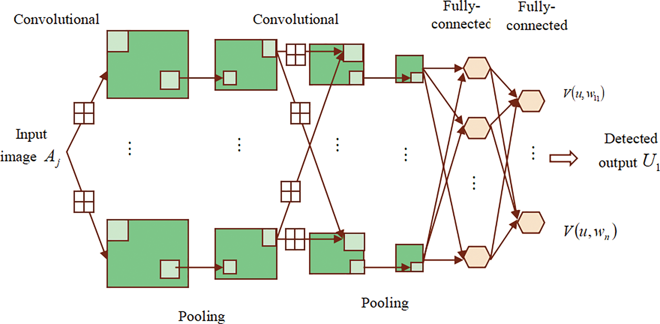
Figure 4: Architectural view of DQN

3.6.2 Jaccard Layer

The Jaccard layer operates on the output of the DQN model U1 and the statistical feature set QS. The Jaccard layer utilizes the Jaccard similarity measure [38] to compute the similarity between the features set. The resultant output is concatenated with the detected output as follows in Eq. (33),

U2=Jacc(QS)||U1(33)

where, Jacc refers to the Jaccard similarity, which is also called as Jaccard index and is applied to gauge the similarity of diverse samples. The Jaccard score is given in Eq. (34),

Jacc(D1,D2)=|D1∩D2||D1∪D2|(34)

Here, D1 and D2 designate the sample sets, and the output U2 is forwarded to the JFDQN for further processing.

3.6.3 JFDQN Layer

The Jaccard layer output U2, feature vector QS, and textual feature image QT are passed to the JFDQN to obtain the final detected output. Here, regression analysis combines all the inputs to yield the final detected output. Regression analysis is applied in this layer by using the FC concept. The FC [42] is a method for solving derivative and integral functions by the Laplace transform. The problem is first solved in the Laplace domain and then the Laplace transform is then applied to obtain the original solution. FC is highly effective in enhancing the performance of various algorithms, including edge detection, pattern matching, filtering, and so on. Here, the various outputs generated at various time instances are utilized to attain the final outcome.

At time t, the output of the JFDQN is generated by considering the LVP feature and is given in Eq. (35),

z=∑i=1v1∑j=1v2Q1∗ωij(35)

Likewise, the output at time instance t−1, the output is produced using the ORB feature, and this is expressed in Eq. (36),

z1=∑i=1v1∑j=1v2Q2∗ωij(36)

where, v1×v2 yields the dimension of the LVP and ORB textual feature, Q1 refers to the LVP feature, Q2 depicts the ORB feature, and ωij denotes the weight. It controls the strength of each feature’s influence in the regression-based output of JFDQN. It is learned during training to optimize detection performance by fusing features more effectively and minimizing the total error.

Similarly, at the time t−2, the output is determined based on the statistical feature set QS and is formulated in Eq. (37),

z2=∑j=15ωiQSi(37)

Further, the output at the time t−3, the Jaccard layer U2 output is taken into account.

Applying in Eq. (38) FC [42],

x(t+1)=gx(t)+12gx(t−1)+16g(1−g)x(t−2)+124g(1−g)(2−g)x(t−3)(38)

Applying the corresponding values of the outputs of the JFDQN layer in Eq. (39),

U3=g∑i=1v1∑j=1v2Q1∗ωij+12g∑i=1v1∑j=1v2Q2∗ωij+16g(1−g)∑j=15ωiQSi+124g(1−g)(2−g)U2(39)

where, g designates the constant associated with the derivative order, and U3 represents the final detected output.

Here, the JDQN is applied with the features obtained from the HS-MS, HS-SAR, and HS-SAR-DSM images and correspondingly, the JDQN produces three outputs X1, X2 and X3, and these three outputs are fed to the DMN for fusion.

3.7 Fusion Using DMN

The three outputs X1, X2 and X3 produced by the JDQN are fed into the DMN for fusion. The DMN fuses these three inputs and produces a fused output representing the final detected output. Here, the process of late fusion is accomplished by the DMN as the individual modal images are subject to detection at first using the JDQN, and the final detected results are aggregated using the DMN. Here, fusion is accomplished using DMN as it is extremely effective even in resource-constrained situations.

Architecture of DMN:

The DMN [40] encompasses numerous maxout layers that produce learnable hidden activations and these layers are linked consecutively. Maxout adopts a maximal operation on the adaptable linear processes and is a general form of Rectified Linear Unit (ReLU). The JDQN outputs X={X1,X2,X3} is applied to the DMN and the following illustrates the operations carried out in the different layers. The following Eqs. (40)–(44) depict how the activations of the hidden layer are determined.

pj,k1=maxk∈[1,q1]XTα…jk+κjk(40)

pj,k2=maxk∈[1,q2]pj,k1Tα…jk+κjk(41)

⋮

pj,kς=maxk∈[1,qς1]pj,kς−1Tα…jk+κjk(42)

⋮

pj,kη=maxk∈[1,qη1]pj,kη−1Tα…jk+κjk(43)

zj=maxk∈[1,qη]pj,kη(44)

Here, η is the layer count of the DMN and qς signifies the amount of units in the ςth layer, zj is the output of the hidden unit, κjk and αjk characterizes the bias and weights, and pj,kς represents the output produced by the ςth layer. DMN utilizes a max-pooling function and hence the maximal output value is fed to the succeeding layers. When the value of κ exceeds 2, then the DMN can approximate any complex non-linear functions. Thus, the DMN produces a fused output ζ based on the detected outputs of the JDQN. The architecture of the DMN is illustrated in Fig. 5.

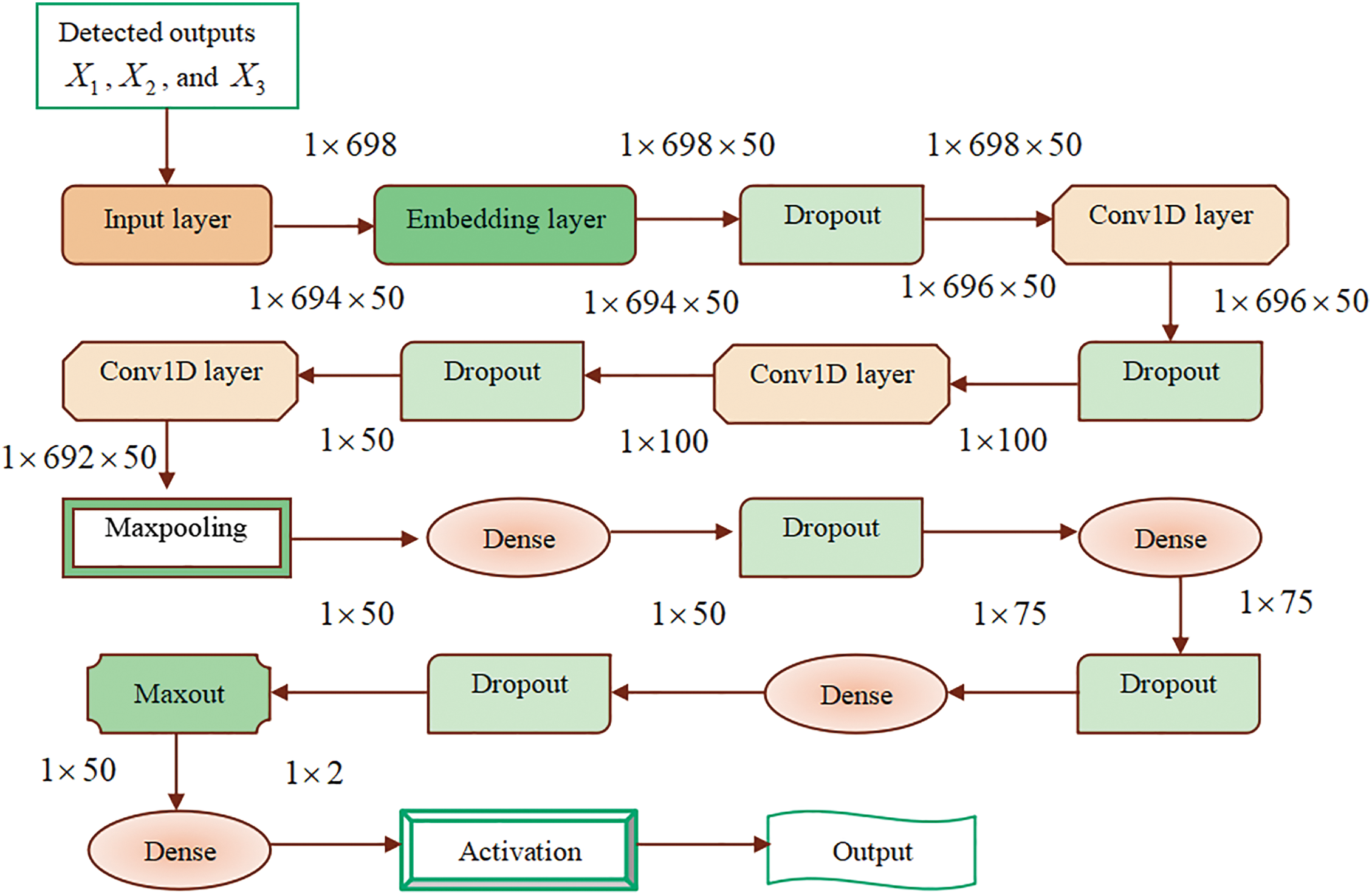
Figure 5: Architecture of DMN

4  Results and Discussion

In this section, the evaluation of the JDQN is conducted using data from the Multimodal Remote Sensing Benchmark Datasets for Land Cover Classification [44] with respect to different parameters to demonstrate the superiority of the method.

4.1 Experimental Set-Up

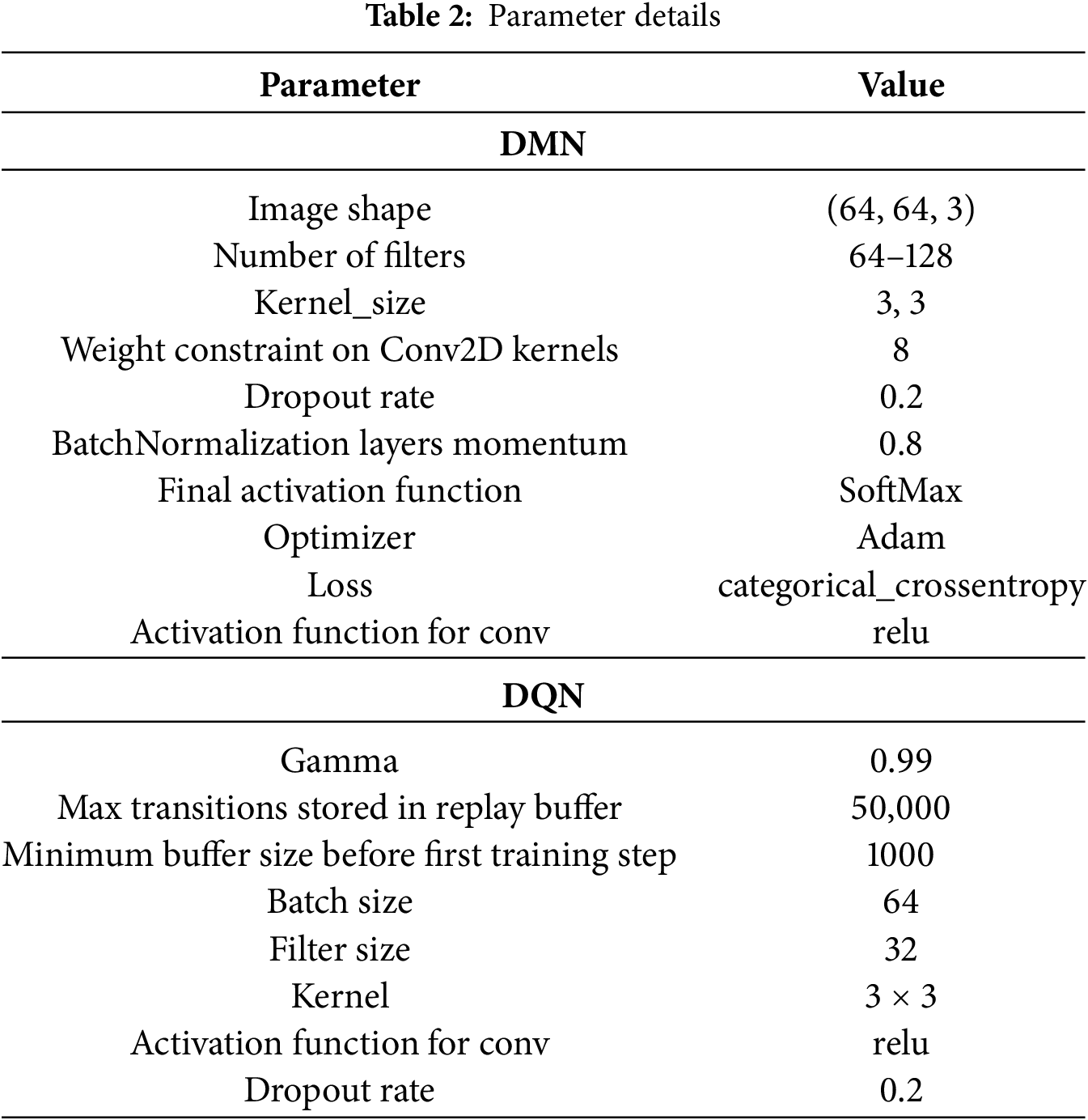
This work proposes a Meyer wavelet transform and Jaccard Deep Q-Net (JDQN)-enabled Deep Maxout Network (DMN) for classifying small objects using multi-modal images, including HS-MS, HS-SAR, and HS-SAR-DSM. The process begins with noise removal using a Kalman filter, followed by image transformation using the Meyer wavelet. The transformed images are segmented using deep joint segmentation and features are extracted using methods like ORB, LVP, and statistical metrics. The extracted features are classified using the newly developed JDQN, which integrates Jaccard similarity and Deep Q-Net. The same workflow is applied to all input image types, and the outputs are processed through the DMN for final classification. The model is implemented in Python, evaluated using performance metrics like PSNR and MSR, and compared with existing methods to highlight its effectiveness. The parameter details of the proposed method are illustrated in Table 2.

4.2 Dataset Description

The multimodal images used in this study are taken from the Multimodal Remote Sensing Benchmark Datasets for Land Cover Classification [44]. The dataset encompasses three multimodal RS datasets, such as HS-SAR-DSM Augsburg, HS-SAR Berlin, and HS-MS Houston 2013. The HS-SAR Berlin dataset comprises the simulated EnMAP data created using the HyMap HS data, explicitly characterizing the rural and urban areas in Berlin urban. The HS-SAR-DSM Augsburg dataset includes data acquired from three distinct sources, such as the DSM image, a dual-Pol PolSAR image, and spaceborne HS image. Here, the POLSAR image is acquired using the Sentinenel-1 and the DSM and HS images are collected using the DAS-EOC over the Augsburg city in Germany. Likewise, the HS-MS Houston2013 is a homogeneous dataset containing HS and MS data acquired from the campus region in the University of Houston, Texas. The dataset consists of images with 1723 × 476 size and includes 244 slices in total.

4.3 Experimental Results

The image outputs obtained during the implementation of the JDQN are illustrated in Fig. 6. Specifically, Fig. 6a represents the input image, Fig. 6b shows the filtered image, Fig. 6c displays the image after applying the Meyer Wavelet Transform (MWT), Fig. 6d portrays the segmented image corresponding to the DSM modality and the ground truth image is included in Fig. 6e.

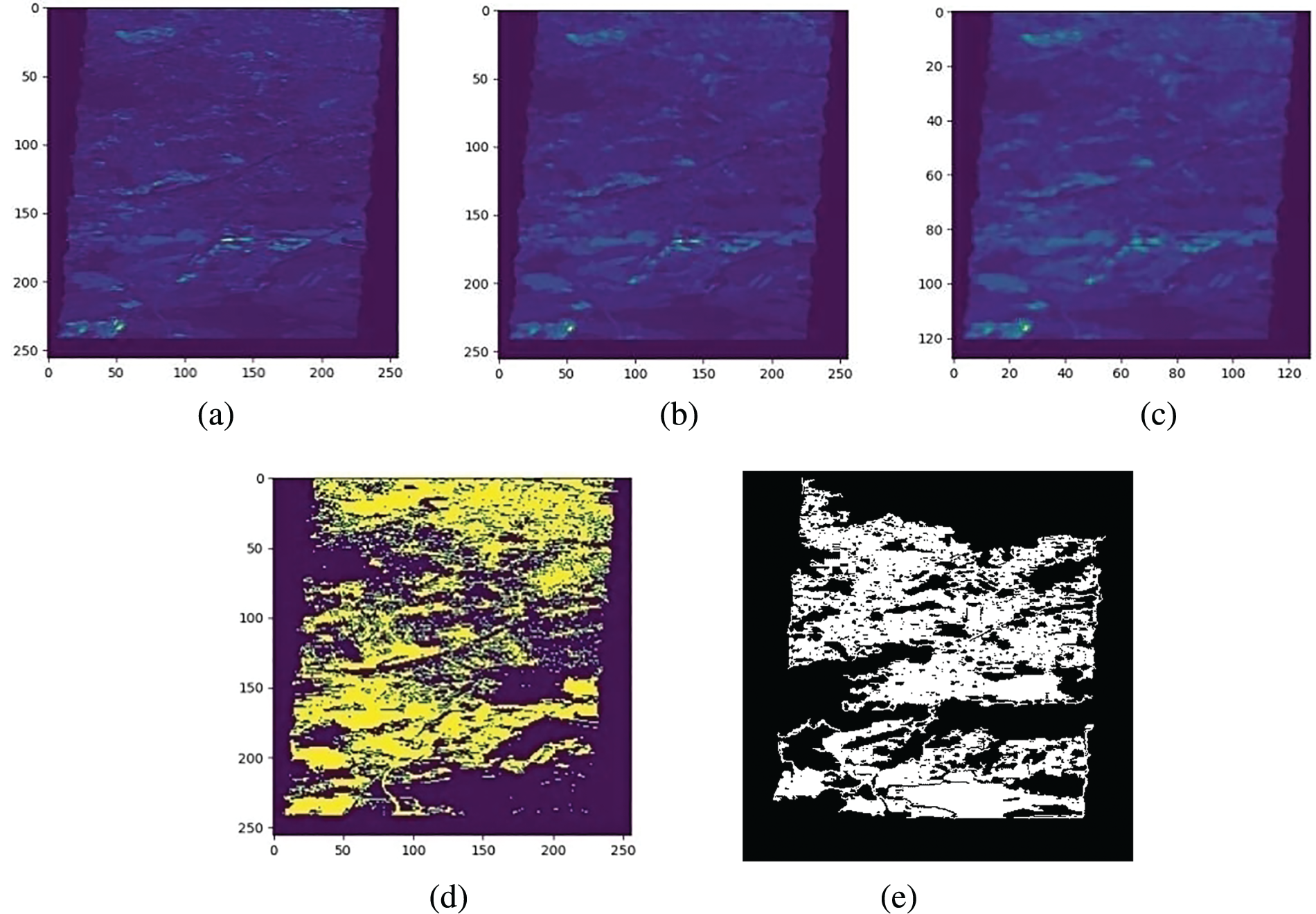
Figure 6: Image results of JDQN for DSM images a) input, b) filtered, c) MWT-applied, d) segmented images, and e) ground truth image

4.4 Evaluation Measures

The JDQN proposed in this research is analysed based on measures, like accuracy, precision, MSE and RMSE.

i) Accuracy: It is used to measure the effectiveness of the JDQN in identifying the small objects correctly and expressed in Eq. (45),

Acc=P1+N1P1+N1+P2+N2(45)

wherein, P1 and N1 symbolize true positive and true negative, P2 and N2 signify false positive and false negative, respectively.

ii) Precision: This factor is employed for determining the ability of the JDQN in producing the same results at various instances, and is expressed in Eq. (46),

Precision=P1P1+P2(46)

iii) MSE: It is used to find the average squared variation of the results produced by JDQN with respect to the expected results, and is expressed in Eq. (47),

MSE=1v∑j=1v(Rv∗−Rv)2(47)

Here, Rv and Rv∗ refer to the actual and the projected output of the JDQN and the term v indicates the samples employed for training the JDQN.

iv) RMSE: The square root of the MSE yields the RMSE value and is formulated as Eq. (48),

RMSE=MSE=1v∑j=1v(Rv∗−Rv)2(48)

Due to high variation in the values measured for MSE, and RMSE, in this work normalized values of these parameters are used. Specifically, Min-Max normalization was applied to scale the raw MSE and RMSE values between 0 and 1. The normalization formula is given as follows:

Normalizedvalue=X−XminXmax−Xmin(49)

Here, the original MSE or RMSE is represented as X and Xmin and Xmax correspond to the minimum and maximum values observed across all compared models and training data splits or K-Fold. This normalization allows for fair visual comparison of model performance trends over varying training data percentages or K-Fold.

4.5 Performance Analysis

The JDQN is scrutinized for its performance with respect to training data at various epochs, and it is illustrated in Fig. 7.

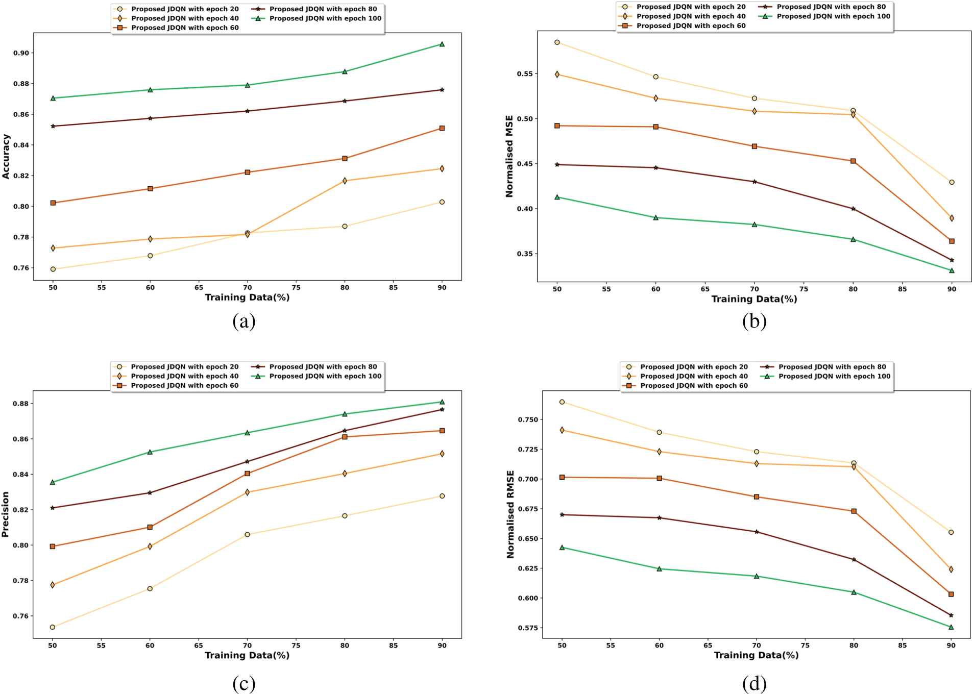
Figure 7: Performance evaluation of the JDQN in terms of a) accuracy, b) normalized MSE, c) precision, and d) normalized RMSE

The analysis of the JDQN concerning accuracy is shown in Fig. 7a. The JDQN recorded accuracy values of 0.783, 0.782, 0.822, 0.862, and 0.879, for 20, 40, 60, 80, and 100 epochs, respectively, with 70% training data. Fig. 7b demonstrates the assessment of the JDQN in terms of normalized MSE. The normalized values of MSE measured by the JDQN for 70% training data are 0.509, 0.508, 0.469, 0.430, and 0.366, for 20, 40, 60, 80, and 100 epochs, respectively. In Fig. 7c, the appraisal of the JDQN based on precision is accomplished. The JDQN attained precision values of 0.806, 0.830, 0.840, 0.847, and 0.863 corresponding to 20, 40, 60, 80, and 100 epochs, respectively, with 70% training data. Further, in Fig. 7d, the examination of the JDQN based on normalized RMSE is illustrated with 70% training data, the JDQN recorded normalized RMSE values of 0.713, 0.713, 0.685, 0.656, and 0.605, for 20, 40, 60, 80, and 100 epochs, respectively.

4.6 Comparative Techniques

The JDQN is compared to the prevailing techniques of small object detection, such as YOLOrs [12], EFPN [26], Faster-RCNN [21], GHOST [5], DLSODC-GWM [9], and CAT-Det [29] to examine its efficiency.

4.7 Comparative Assessment

The investigation of the JDQN is accomplished by taking into consideration the values recorded for various parameters with diverse training data and K-Fold.

4.7.1 Based on Training Data

Fig. 8 examines the small objection detection framework proposed in this work with varying percentages of training data. The assessment of the JDQN in terms of accuracy is depicted in Fig. 8a. The different small object detection approaches, such as YOLOrs, EFPN, Faster-RCNN, GHOST, DLSODC-GWM, CAT-Det, and JDQN are observed to measure the accuracy of 0.798, 0.849, 0.864, 0.879, 0.831, 0.856, and 0.884, correspondingly, for 80% training data. This demonstrates that the JDQN achieved a better accuracy value of 9.73%, 3.96%, 2.56%, 0.56%, 6.00%, and 3.17% than the existing techniques. Fig. 8b illustrates the evaluation of the JDQN in terms of normalized MSE. For 60% of training data, the normalized MSE recorded by the JDQN is 0.393, while the existing techniques produced normalized MSE values of 0.533 for YOLOrs, 0.526 for EFPN, 0.463 for Faster-RCNN, 0.438 for GHOST, 0.535 for DLSODC-GWM, 0.495 for CAT-Det. Fig. 8c presents the analysis of the JDQN based on precision. The precision value recorded by the object detection approaches, like YOLOrs is 0.839, EFPN is 0.862, Faster-RCNN is 0.877, GHOST is 0.892, DLSODC-GWM is 0.859, CAT-Det is 0.876, and JDQN is 0.902 with 80% training data. Thus, the JDQN demonstrated an improved performance of 7.05%, 4.47%, 2.76%, 1.17%, 4.77%, and 2.88% than the existing methods. Likewise, the investigation of the JDQN in view of the normalized RMSE is displayed in Fig. 8d. The normalized value of RMSE attained by the JDQN is 0.627, which is lower than the normalized RMSE value of 0.730, 0.725, 0.680, 0.662, 0.735, and 0.706 measured by the YOLOrs, EFPN, Faster-RCNN, GHOST, DLSODC-GWM, and CAT-Det, respectively, with 60% of training data. Fig. 8e depicts the analysis of the inference time. The inference time required by the object detection approaches, like YOLOrs is 0.137 ms, EFPN is 0.114 ms, Faster-RCNN is 0.105 ms, GHOST is 0.103 ms, DLSODC-GWM is 0.102 ms, CAT-Det is 0.095 ms, and JDQN is 0.078 ms with 90% of training data.

Figure 8: Comparative valuation of the JDQN considering a) accuracy, b) normalized MSE, c) precision, d) normalized RMSE, and e) inference time with varying training data

4.7.2 Using K-Fold Cross Validation

Fig. 9 provides an evaluation of the JDQN model based on four performance metrics, considering the K-Fold. In Fig. 9a, the performance of JDQN in terms of accuracy is illustrated. The competing methods, including YOLOrs, EFPN, Faster-RCNN, GHOST, DLSODC-GWM, and CAT-Det, achieved accuracy levels of 0.821, 0.859, 0.874, 0.889, 0.848, and 0.869, respectively. The JDQN achieved a higher accuracy of 0.899 with a K-Fold of 8, which is 8.69%, 4.49%, 2.77%, 1.17%, 5.67%, and 3.34% improved than the existing methods. Fig. 9b presents the normalized MSE analysis of JDQN. At a K-Fold of 6, JDQN demonstrated a lower normalized MSE of 0.382, while the values recorded by YOLOrs, EFPN, Faster-RCNN, GHOST, DLSODC-GWM, and CAT-Det, were 0.543, 0.476, 0.409, 0.384, 0.529, and 0.493, respectively, showcasing JDQN’s enhanced performance in minimizing MSE. The precision of JDQN is analyzed in Fig. 9c. For a K-Fold of 8, the precision values achieved by YOLOrs, EFPN, Faster-RCNN, GHOST, DLSODC-GWM, CAT-Det, and JDQN were 0.830, 0.861, 0.876, 0.891, 0.854, 0.873, and 0.896, respectively. This indicates that JDQN outperformed the other methods, with improvements of 7.36%, 3.93%, 2.21%, 0.61%, 4.69%, and 2.57%. Fig. 9d illustrates the normalized RMSE performance of JDQN. At a K-Fold of 6, the normalized RMSE values recorded were 0.737 for YOLOrs, 0.690 for EFPN, 0.640 for Faster-RCNN, 0.620 for GHOST, 0.731 for DLSODC-GWM, 0.705 for CAT-Det, and a superior 0.618 for JDQN, highlighting its effectiveness and superiority across all metrics.

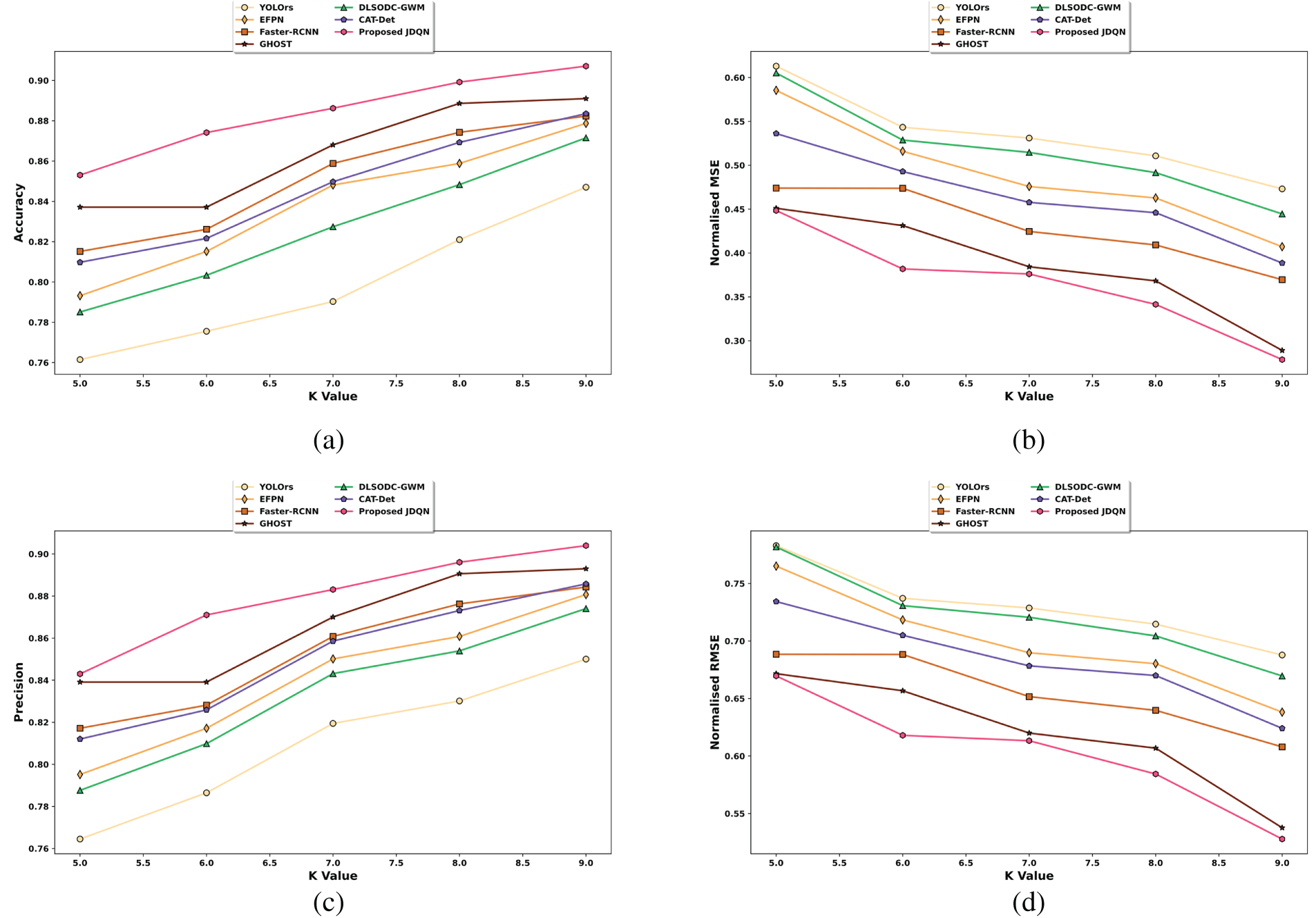
Figure 9: Comparative analysis of the JDQN concerning a) accuracy, b) normalized MSE, c) precision, and d) normalized RMSE based on K-Fold

4.8 Ablation Study

Fig. 10 illustrates the results of an ablation study conducted to evaluate the contribution of each component within the proposed JDQN framework, using accuracy as the performance metric. This analysis is performed by systematically removing individual components and observing the resulting changes in accuracy across different proportions of training data. When 90% of the training data is considered, the accuracy obtained by the JDQN without AKF, JDQN without MWT, JDQN without Deepjoint segmentation, JDQN without feature extraction, DQN, and proposed JDQN is 0.812, 0.851, 0.855, 0.863, 0.884, and 0.902. These findings underscore the significance of each component in enhancing the overall accuracy of the proposed model.

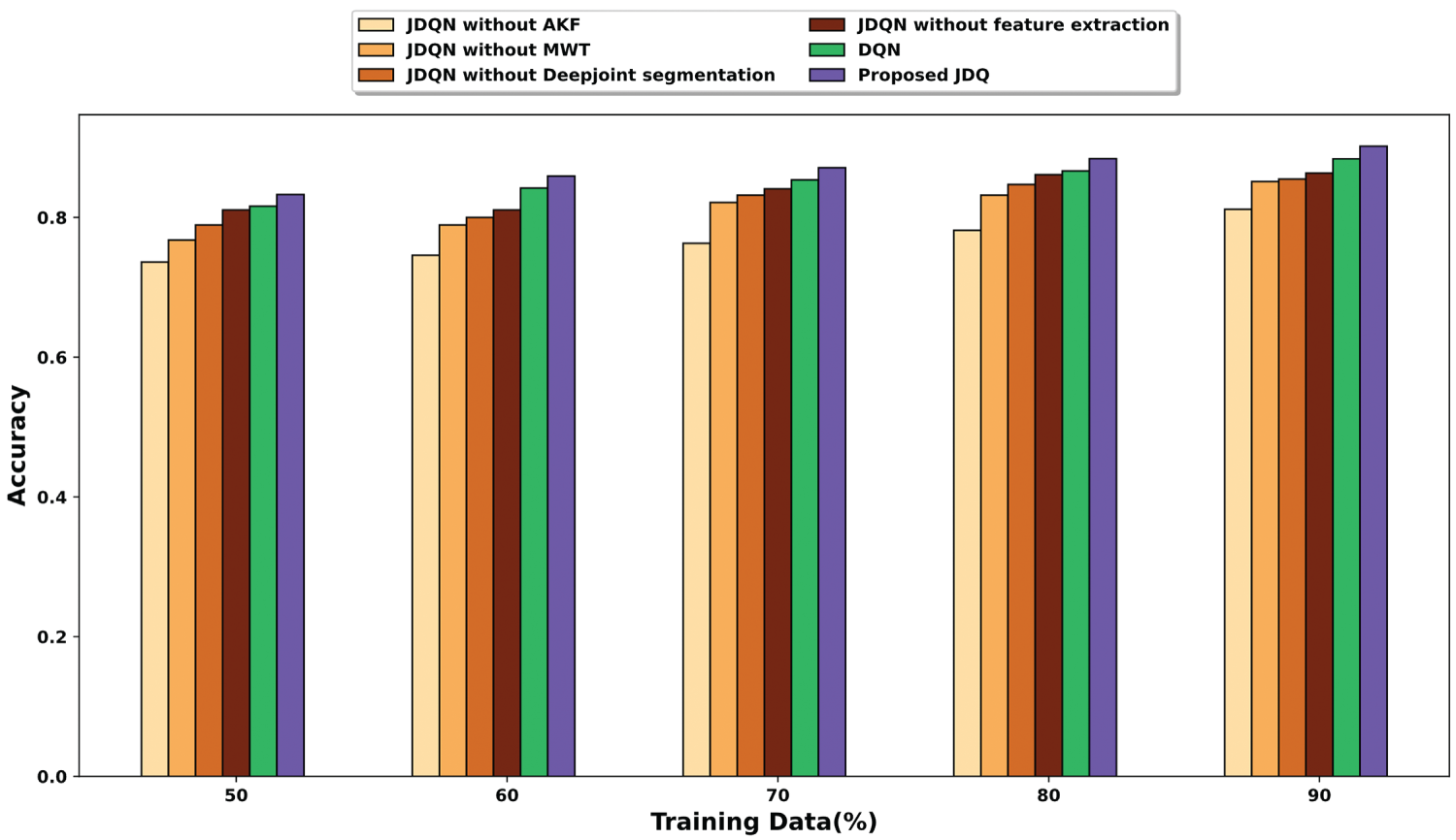
Figure 10: Ablation study

4.9 Analysis Based on Fusion

Fig. 11 presents a comparative analysis of different fusion strategies. In this research, DMN is used for fusion, and the performance of the DMN is compared with other fusion methods, such as averaging and majority voting. As illustrated in the figure, the JDQN with DMN consistently achieves higher accuracy across all training data percentages. When 90% of the training data is used, the accuracy obtained by JDQN with averaging, JDQN with majority voting, and JDQN with DMN is 0.827, 0.868, and 0.890, respectively. These results indicate that the DMN-based fusion significantly improves the ability to integrate multimodal information, leading to more accurate small object detection.

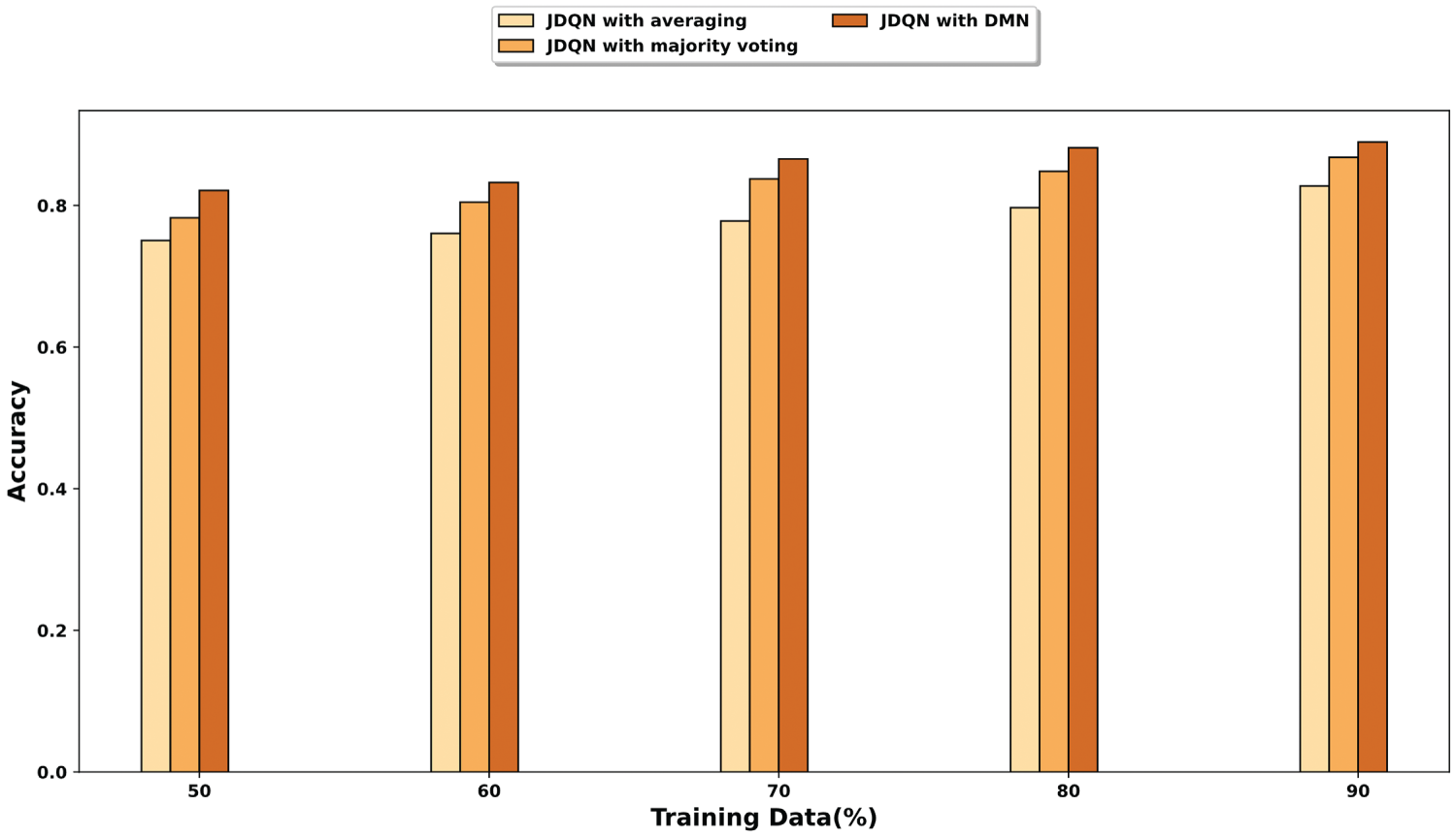
Figure 11: Analysis based on fusion

4.10 Statistical Analysis

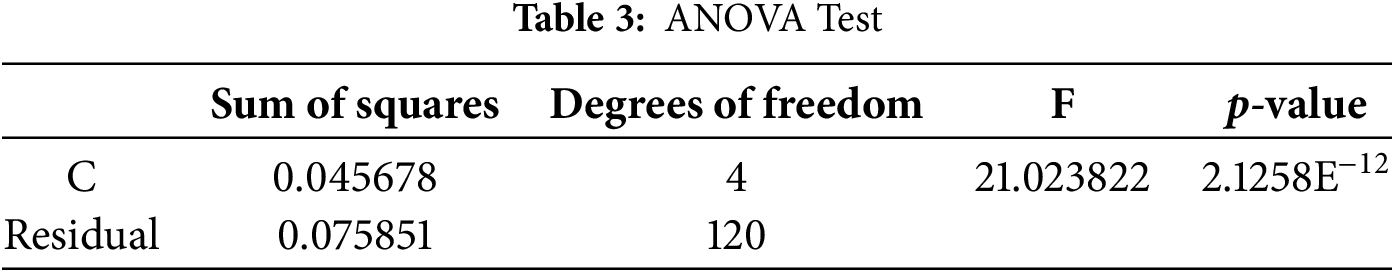
Table 3 presents the results of the Analysis of Variance (ANOVA) test conducted to evaluate the statistical significance of differences in performance among the various methods analyzed. The factor C, representing the comparison groups, shows a sum of squares of 0.045678 with 4 degrees of freedom, resulting in an F-value of 21.023822. The associated p-value is 2.1258E−12, which is significantly lower than the conventional significance threshold 0.05. These results indicate that there is a statistically significant difference among the compared methods. Additionally, the 95% confidence interval for accuracy, ranging from 0.8266 to 0.9123, reinforces the robustness and reliability of the proposed model.

4.11 Comparative Discussion

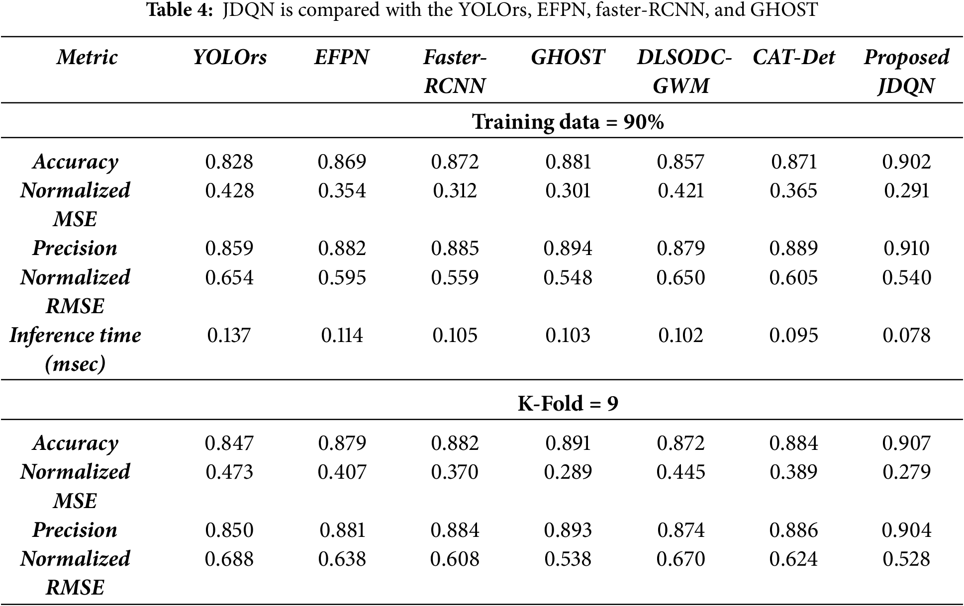
In Table 4, the comparison of JDQN with YOLOrs, EFPN, Faster-RCNN, and GHOST is presented in terms of accuracy, normalized MSE, precision, and normalized RMSE. The values in Table 4 correspond to the scenario when 90% of the training data and a K-Fold of 9 are considered. It can be noticed from the table that the JDQN achieved a higher accuracy of 0.907, whereas the accuracy measured by YOLOrs is 0.847, EFPN is 0.879, Faster-RCNN is 0.882, GHOST is 0.891, DLSODC-GWM is 0.872, and CAT-Det is 0.884. The high accuracy is attributed to the minimization of false positives due to the capability of JDQN in learning high-level representations in the input image. Likewise, the JDQN achieved a high precision of 0.904 as a result of the application of Deepjoint segmentation for extricating the small objects from the background. The approaches, such as YOLOrs, EFPN, Faster-RCNN, GHOST, DLSODC-GWM, and CAT-Det, however, recorded a low precision of 0.850, 0.881, 0.884, 0.893, 0.874, and 0.886, respectively. Similarly, the JDQN recorded a lower normalized MSE value of 0.279 in comparison to the normalized MSE measured by YOLOrs is 0.473, EFPN is 0.407, Faster-RCNN is 0.370, GHOST is 0.289, DLSODC-GWM is 0.445, and CAT-Det is 0.389. The application of ORB and LVP features enabled the extraction of optimal features, which contributed to minimal error while detecting small objects. The low value of normalized MSE of the JDQN also led to a low normalized RMSE value of 0.528, whereas the normalized RMSE attained by YOLOrs, EFPN, Faster-RCNN, GHOST, DLSODC-GWM, and CAT-Det is 0.688, 0.638, 0.608, 0.538, 0.670, and 0.624, respectively. The proposed method achieved an inference time of 0.078 ms, which is lower than that of the compared methods when considering training data is 90%.

The superior performance of the proposed method stems from its effective integration of multimodal image data, leveraging complementary information to address challenges such as low resolution, occlusion, and background interference. The JDQN combines the Jaccard similarity measure with DQN to enhance object localization and adapt to varying conditions, while regression modeling further refines predictions. Additionally, the DMN efficiently fuses outputs from different modalities, ensuring robust final detection. The high performance of the proposed method underscores its reliability in detecting small objects.

4.12 Practical Applications

The proposed JDQN-based small object detection framework holds significant potential for practical deployment in real-world scenarios. In military surveillance, the integration of hyperspectral and SAR data enables the accurate identification of hidden objects under challenging environmental conditions. Similarly, in emergency rescue operations, rapid and reliable detection of small objects in cluttered environments can greatly enhance response efficiency and safety. Beyond these domains, the JDQN framework is adaptable to urban monitoring, border surveillance, disaster management, and environmental monitoring, where multimodal data sources are often available.

5  Conclusion

In this research, a deep learning (DL) network named JDQN is proposed for detecting small objects from multimodal remote sensing (RS) images. The JDQN is developed by integrating the Jaccard similarity measure into the Deep Q-Network (DQN) framework, leveraging regression analysis. The detection process involves a sequence of steps, including pre-processing, image transformation, segmentation, feature extraction, detection, and fusion. Multimodal input images, such as HS-SAR, HS-MS, or HS-SAR-DSM, are initially denoised using the Adaptive Kalman Filter (AKF) and subsequently transformed into the frequency domain using the Meyer Wavelet Transform (MWT). Following this, small objects are segmented from the background using Deepjoint segmentation, and various features are extracted. These features are then fed into the JDQN to detect small objects, with the results from each modality fused using the DMN to produce the final output. The proposed JDQN demonstrates superior performance, achieving an accuracy of 0.907, a normalized MSE of 0.279, a precision of 0.904, and a normalized RMSE of 0.528. Future work will aim to further enhance detection accuracy through the integration of advanced image augmentation techniques and additional features, increasing the approach’s applicability to real-time scenarios. The feasibility of deploying JDQN in real-time systems, such as drones for surveillance or emergency response, as well as the extension of the method to additional imaging modalities, such as thermal or ultrasound imaging, will be explored in future work.

Acknowledgement: The authors would like to thank all individuals and institutions that contributed to this research.

Funding Statement: Princess Nourah bint Abdulrahman University Researchers Supporting Project number (PNURSP2025R137), Princess Nourah bint Abdulrahman University, Riyadh, Saudi Arabia. The authors extend their appreciation to Universiti Teknikal Malaysia Melaka (UTeM) and to the Ministry of Higher Education of Malaysia (MOHE) for their support in this research. The authors express their gratitude to Quanzhou University of Information Engineering for its support in this research.

Author Contributions: Mian Muhammad Kamal: Conceptualization, Methodology, Writing—original draft, Investigation. Syed Zain Ul Abideen: Writing—original draft, Investigation. M. A. Al-Khasawneh: Software, Writing—review & editing. Alaa M. Momani: Data curation, Investigation. Hala Mostafa; Funding acquisition, Supervision, Project administration. Mohammed Salem Atoum: Project administration, Supervision. Saeed Ullah: Validation, Software. Jamil Abedalrahim Jamil Alsayaydeh: Supervision, Funding acquisition, Project administration. Mohd Faizal Bin Yusof: Conceptualization, Writing—review & editing. Suhaila Binti Mohd Najib: Data curation, Writing—review & editing. All authors reviewed the results and approved the final version of the manuscript.

Availability of Data and Materials: The data that support the findings of this study are available from the corresponding authors upon reasonable request.

Ethics Approval: Not applicable.

Conflicts of Interest: The authors declare no conflicts of interest to report regarding the present study.

References

1. Meyer A, Brand F, Kaup A. Learned wavelet video coding using motion compensated temporal filtering. IEEE Access. 2023;11:113390–401. doi:10.1109/ACCESS.2023.332387. [Google Scholar] [CrossRef]

2. Ding J, Xue N, Long Y, Xia GS, Lu Q. Learning RoI transformer for oriented object detection in aerial images. In: IEEE/CVF Conference on Computer Vision and Pattern Recognition (CVPR); 2019 Jun 15–20; Long Beach, CA, USA. p. 2844–53. doi:10.1109/CVPR.2019.00296. [Google Scholar] [CrossRef]

3. Bhanu B, Lin Y. Object detection in multi-modal images using genetic programming. Appl Soft Comput. 2004;4(2):175–201. doi:10.1016/j.asoc.2004.01.004. [Google Scholar] [CrossRef]

4. Wang Z, Zang T, Fu Z, Yang H, Du W. RLPGB-net: reinforcement learning of feature fusion and global context boundary attention for infrared dim small target detection. IEEE Trans Geosci Remote Sens. 2023;61:5003615. doi:10.1109/TGRS.2023.3304755. [Google Scholar] [CrossRef]

5. Zhang J, Lei J, Xie W, Li Y, Yang G, Jia X. Guided hybrid quantization for object detection in remote sensing imagery via one-to-one self-teaching. IEEE Trans Geosci Remote Sens. 2023;61:5614815. doi:10.1109/TGRS.2023.3293147. [Google Scholar] [CrossRef]

6. Zhang C, Achuthan A, Himel GMS. State-of-the-art and challenges in pancreatic CT segmentation: a systematic review of U-Net and its variants. IEEE Access. 2024;12(2):78726–42. doi:10.1109/access.2024.3392595. [Google Scholar] [CrossRef]

7. Wang H, Zhou L, Wang L. Miss detection vs. false alarm: adversarial learning for small object segmentation in infrared images. In: 2019 IEEE/CVF International Conference on Computer Vision (ICCV); 2019 Oct 27–Nov 2; Seoul, Republic of Korea. p. 8508–17. doi:10.1109/iccv.2019.00860. [Google Scholar] [CrossRef]

8. Chandra Joshi R, Kumar Sharma A, Kishore Dutta M. VisionDeep-AI: deep learning-based retinal blood vessels segmentation and multi-class classification framework for eye diagnosis. Biomed Signal Process Control. 2024;94:106273. doi:10.1016/j.bspc.2024.106273. [Google Scholar] [CrossRef]

9. Alsubaei FS, Al-Wesabi FN, Hilal AM. Deep learning-based small object detection and classification model for garbage waste management in smart cities and IoT environment. Appl Sci. 2022;12(5):2281. doi:10.3390/app12052281. [Google Scholar] [CrossRef]

10. Tian Y, Wang K, Wang Y, Tian Y, Wang Z, Wang FY. Adaptive and azimuth-aware fusion network of multimodal local features for 3D object detection. Neurocomputing. 2020;411(3):32–44. doi:10.1016/j.neucom.2020.05.086. [Google Scholar] [CrossRef]

11. Taye MM. Understanding of machine learning with deep learning: architectures, workflow, applications and future directions. Computers. 2023;12(5):91. doi:10.3390/computers12050091. [Google Scholar] [CrossRef]

12. Sharma M, Dhanaraj M, Karnam S, Chachlakis DG, Ptucha R, Markopoulos PP, et al. YOLOrs: object detection in multimodal remote sensing imagery. IEEE J Sel Top Appl Earth Obs Remote Sens. 2020;14:1497–508. doi:10.1109/jstars.2020.3041316. [Google Scholar] [CrossRef]

13. Liu L, Ouyang W, Wang X, Fieguth P, Chen J, Liu X, et al. Deep learning for generic object detection: a survey. Int J Comput Vis. 2020;128(2):261–318. doi:10.1007/s11263-019-01247-4. [Google Scholar] [CrossRef]

14. Zhao ZQ, Zheng P, Xu ST, Wu X. Object detection with deep learning: a review. IEEE Trans Neural Netw Learn Syst. 2019;30(11):3212–32. doi:10.1109/TNNLS.2018.2876865. [Google Scholar] [PubMed] [CrossRef]

15. Han J, Zhang D, Cheng G, Liu N, Xu D. Advanced deep-learning techniques for salient and category-specific object detection: a survey. IEEE Signal Process Mag. 2018;35(1):84–100. doi:10.1109/MSP.2017.2749125. [Google Scholar] [CrossRef]

16. Park CW, Seo Y, Sun TJ, Lee GW, Huh EN. Small object detection technology using multi-modal data based on deep learning. In: 2023 International Conference on Information Networking (ICOIN); 2023 Jan 11–14; Bangkok, Thailand. p. 420–2. doi:10.1109/ICOIN56518.2023.10049014. [Google Scholar] [CrossRef]

17. Yin Z, Wu Z, Zhang J. A deep network based on wavelet transform for image compressed sensing. Circuits Syst Signal Process. 2022;41(11):6031–50. doi:10.1007/s00034-022-02058-8. [Google Scholar] [CrossRef]

18. Al-Battal AF, Gong Y, Xu L, Morton T, Du C, Bu Y, et al. A CNN segmentation-based approach to object detection and tracking in ultrasound scans with application to the vagus nerve detection. In: 2021 43rd Annual International Conference of the IEEE Engineering in Medicine & Biology Society (EMBC); 2021 Nov 1–5; Mexico. p. 3322–7. doi:10.1109/EMBC46164.2021.9630522. [Google Scholar] [PubMed] [CrossRef]

19. Sipai U, Jadeja R, Kothari N, Trivedi T, Mahadeva R, Patole SP. Performance evaluation of discrete wavelet transform and machine learning based techniques for classifying power quality disturbances. IEEE Access. 2024;12:95472–86. doi:10.1109/access.2024.3426039. [Google Scholar] [CrossRef]

20. Li X, Liu J, Tang Z, Han B, Wu Z. MEDMCN: a novel multi-modal EfficientDet with multi-scale CapsNet for object detection. J Supercomput. 2024;80(9):12863–90. doi:10.1007/s11227-024-05932-1. [Google Scholar] [CrossRef]

21. Cao C, Wang B, Zhang W, Zeng X, Yan X, Feng Z, et al. An improved faster R-CNN for small object detection. IEEE Access. 2019;7:106838–46. doi:10.1109/access.2019.2932731. [Google Scholar] [CrossRef]

22. Condat R, Rogozan A, Bensrhair A. GFD-retina: gated fusion double RetinaNet for multimodal 2D road object detection. In: 2020 IEEE 23rd International Conference on Intelligent Transportation Systems (ITSC); 2020 Sep 20–23; Rhodes, Greece. p. 1–6. doi:10.1109/itsc45102.2020.9294447. [Google Scholar] [CrossRef]

23. Chen D, Zhao H, Li Y, Zhang Z, Zhang K. PMF-YOLOv8: enhanced ship detection model in remote sensing images. Inf Technol Control. 2024;53(4):1204–20. doi:10.5755/j01.itc.53.4.37003. [Google Scholar] [CrossRef]

24. Pan W, Shi H, Zhao Z, Zhu J, He X, Pan Z, et al. Wnet: audio-guided video object segmentation via wavelet-based cross-modal denoising networks. In: IEEE/CVF Conference on Computer Vision and Pattern Recognition (CVPR); 2022 Jun 18–24; New Orleans, LA, USA. p. 1310–21. doi:10.1109/CVPR52688.2022.00138. [Google Scholar] [CrossRef]

25. Punn NS, Agarwal S. Modality specific U-Net variants for biomedical image segmentation: a survey. Artif Intell Rev. 2022;55(7):5845–89. doi:10.1007/s10462-022-10152-1. [Google Scholar] [PubMed] [CrossRef]

26. Deng C, Wang M, Liu L, Liu Y, Jiang Y. Extended feature pyramid network for small object detection. IEEE Trans Multimed. 2021;24:1968–79. doi:10.1109/TMM.2021.3074273. [Google Scholar] [CrossRef]

27. Zhang J, Lei J, Xie W, Fang Z, Li Y, Du Q. SuperYOLO: super resolution assisted object detection in multimodal remote sensing imagery. IEEE Trans Geosci Remote Sens. 2023;61:5605415. doi:10.1109/TGRS.2023.3258666. [Google Scholar] [CrossRef]

28. Saeed F, Ahmed MJ, Gul MJ, Hong KJ, Paul A, Kavitha MS. A robust approach for industrial small-object detection using an improved faster regional convolutional neural network. Sci Rep. 2021;11(1):23390. doi:10.1038/s41598-021-02805-y. [Google Scholar] [PubMed] [CrossRef]

29. Zhang Y, Chen J, Huang D. CAT-det: contrastively augmented transformer for multimodal 3D object detection. In: IEEE/CVF Conference on Computer Vision and Pattern Recognition (CVPR); 2022 Jun 18–24; New Orleans, LA, USA. p. 898–907. doi:10.1109/CVPR52688.2022.00098. [Google Scholar] [CrossRef]

30. Nan G, Zhao Y, Fu L, Ye Q. Object detection by channel and spatial exchange for multimodal remote sensing imagery. IEEE J Sel Top Appl Earth Obs Remote Sens. 2024;17:8581–93. doi:10.1109/jstars.2024.3388013. [Google Scholar] [CrossRef]

31. Jiang C, Ren H, Yang H, Huo H, Zhu P, Yao Z, et al. M2FNet: multi-modal fusion network for object detection from visible and thermal infrared images. Int J Appl Earth Obs Geoinf. 2024;130:103918. doi:10.1016/j.jag.2024.103918. [Google Scholar] [CrossRef]

32. Mahjourian N, Nguyen V. Multimodal object detection using depth and image data for manufacturing parts. arXiv: 2411.09062. 2024. doi:10.48550/arXiv.2411.09062. [Google Scholar] [CrossRef]

33. Yang Y, Gao W. An optimal adaptive Kalman filter. J Geod. 2006;80(4):177–83. doi:10.1007/s00190-006-0041-0. [Google Scholar] [CrossRef]

34. Valenzuela V, Oliveira H. Close expressions for Meyer wavelet and scale function. In: Anais de XXXIII Simpósio Brasileiro de Telecomunicações. Sociedade Brasileira de Telecomunicações; 2015 Dec 1—4; Brazil: Juiz de Fora. doi:10.14209/sbrt.2015.2. [Google Scholar] [CrossRef]

35. Ali S, Li J, Pei Y, Khurram R, Rehman KU, Mahmood T. A comprehensive survey on brain tumor diagnosis using deep learning and emerging hybrid techniques with multi-modal MR image. Arch Comput Meth Eng. 2022;29(7):4871–96. doi:10.1007/s11831-022-09758-z. [Google Scholar] [CrossRef]

36. Gupta S, Kumar M, Garg A. Improved object recognition results using SIFT and ORB feature detector. Multimed Tools Appl. 2019;78(23):34157–71. doi:10.1007/s11042-019-08232-6. [Google Scholar] [CrossRef]

37. Fan KC, Hung TY. A novel local pattern descriptor—local vector pattern in high-order derivative space for face recognition. IEEE Trans Image Process. 2014;23(7):2877–91. doi:10.1109/tip.2014.2321495. [Google Scholar] [PubMed] [CrossRef]

38. Meyer A, Prativadibhayankaram S, Kaup A. Efficient learned wavelet image and video coding. In: 2024 IEEE International Conference on Image Processing (ICIP); 2024 Oct 27–30; Abu Dhabi, United Arab Emirates. p. 1753–9. doi:10.1109/ICIP51287.2024.10647966. [Google Scholar] [CrossRef]

39. Lv P, Wang X, Cheng Y, Duan Z. Stochastic double deep Q-network. IEEE Access. 2019;7:79446–54. doi:10.1109/access.2019.2922706. [Google Scholar] [CrossRef]

40. Sun W, Su F, Wang L. Improving deep neural networks with multi-layer maxout networks and a novel initialization method. Neurocomputing. 2018;278(9):34–40. doi:10.1016/j.neucom.2017.05.103. [Google Scholar] [CrossRef]

41. Lessa V, Marengoni M. Applying artificial neural network for the classification of breast cancer using infrared thermographic images. Cham, Switzerland: Springer International Publishing; 2016. p. 429–38. doi:10.1007/978-3-319-46418-3_38. [Google Scholar] [CrossRef]

42. Yang Q, Chen D, Zhao T, Chen Y. Fractional calculus in image processing: a review. Fract Calc Appl Anal. 2016;19(5):1222–49. doi:10.1515/fca-2016-0063. [Google Scholar] [CrossRef]

43. Sasaki H, Horiuchi T, Kato S. A study on vision-based mobile robot learning by deep Q-network. In: 2017 56th Annual Conference of the Society of Instrument and Control Engineers of Japan (SICE); 2017 Sep 19–22; Kanazawa, Japan. p. 799–804. [Google Scholar]

44. Hong D, Hu J, Yao J, Chanussot J, Zhu XX. Multimodal remote sensing benchmark datasets for land cover classification with a shared and specific feature learning model. ISPRS J Photogramm Remote Sens. 2021;178(9–10):68–80. doi:10.1016/j.isprsjprs.2021.05.011. [Google Scholar] [PubMed] [CrossRef]