AI for Cleaner Air: Predictive Modeling of PM2.5 Using Deep Learning and Traditional Time-Series Approaches

1  Introduction

Due to fast industrial growth, many people have moved to cities for better jobs and life. This has led to more vehicles and factories that burn fuels such as gasoline and diesel, releasing harmful pollutants. The most dangerous is PM2.5—tiny particles in size (≤2.5 µg/m3) that can enter deep into our lungs when we breathe [1,2].

Air pollution is now a serious global problem [3]. Breathing PM2.5 for long periods causes lung diseases like asthma and bronchitis [4]. It also creates fog, reducing visibility, and causing traffic problems [5]. To fight this, scientists are developing better air quality prediction systems. These help governments make smarter policies [6] and protect public health [7]. Many cities now use sensor networks to monitor PM2.5 and other pollutants like ozone, oxides of nitrogen, Nitrogen dioxide and sulpher dioxide. This is crucial because long-term PM2.5 exposure increases health risks [8].

Air quality prediction models are generally categorized into deterministic methods, statistical methods, and deep learning-based models [9]. The deterministic models are based on numerical simulations of the dispersion of pollutants based on aerodynamic theories. These models include well-known frameworks such as Chemical Transport Models (CTMs) [10], the Nested Air Quality Prediction Modeling System (NAQPMS) [11], and Community Multiscale Air Quality (CMAQ) [12] to name some. Moreover, the accuracy of these models is often limited by uncertainties in parameter selection and a lack of real-time observational data [13]. Additionally, these models require significant computational resources, making large-scale implementations challenging [14].

On the other hand, statistical methods use historical pollutant observations to predict future air quality levels. Traditional statistical models such as autoregressive distributed lag (ARDL) [15], autoregressive integrated moving average (ARIMA) [16], and autoregressive moving average (ARMA) [17] have been widely utilized. However, these models assume a linear relationship between input variables and air pollution levels, which does not align with the inherently nonlinear and dynamic nature of air pollution processes, thereby limiting their predictive performance.

Despite numerous advances in air pollution forecasting, most existing models either rely on traditional statistical techniques like ARIMA, which assume linearity and stationarity, or utilize deep learning architectures that focus solely on either spatial or temporal features. However, standalone models such as CNNs and LSTMs often fail to capture the full complexity of air quality dynamics, especially in the presence of noisy or outlier-prone data. Furthermore, limited studies provide a systematic, head-to-head comparison between traditional statistical baselines and modern deep learning approaches under a unified experimental framework. In particular, hybrid architectures that integrate both spatial and temporal learning components have been underexplored in PM2.5 prediction, and there is little research on how such models perform across different air quality categories (e.g., Good, Satisfactory, Unhealthy) using hourly resolution data.

Existing studies often overlook correlation-based analysis and fail to incorporate systematic feature selection, resulting in models that are less effective in capturing complex pollutant interactions. Additionally, the absence of robust outlier detection in prior work leads to reduced accuracy and increased vulnerability to noise in real-world datasets. This study addresses these limitations by implementing Spearman correlation to extract meaningful features and applying outlier detection to identify and exclude anomalous data points. This approach enhances model robustness, improves predictive accuracy, and reduces computational complexity. The refined dataset is then used to train a hybrid CNN-LSTM model, benchmarked against ARIMA, MLE, and standalone deep learning models using both classification and regression metrics.

A detailed discussion of the statistical and deep-learning-based algorithms is provided in the subsequent section.

2  Literature Review

This section critically examines statistical and deep learning models for air quality prediction, the two most widely adopted data-driven approaches in recent research. Deep learning techniques excel at capturing complex spatiotemporal patterns but require substantial computational resources, while statistical methods offer interpretability and efficiency for linear relationships. The following subsections analyze their respective architectures, applications, and limitations in pollutant forecasting.

Deep learning-based air quality prediction models can be broadly categorized into two groups: forecasting models and classification models. The first category includes temporal architectures such as recurring neural networks (RNNs) and long-short-term memory (LSTM) networks, which capture sequential dependencies on pollutant trends [18]. Variants such as Bidirectional LSTM (BiLSTM) and graph-based LSTMs further enhance accuracy by modeling spatial relationships and bidirectional temporal dynamics. The second category comprises models that extract features from tabular data or remote sensing imagery, classifying pollution levels through convolutional neural networks (CNN) [19]. Hybrid frameworks (e.g., CNN-LSTM) integrate spatial feature extraction with temporal modeling, achieving superior performance in real-world forecasting tasks [20].

Statistical approaches rely on mathematical formulations to predict air quality, falling into three subcategories: (1) linear regression models (e.g., Auto-Regressive Distributed Lag, ARDL) that quantify meteorological variable impacts; (2) time-series methods (e.g., ARIMA, ARMA) for trend prediction, though limited by linearity assumptions; and (3) ensemble techniques (e.g., Random Forest, XGBoost) that combine weak predictors for robust outputs. While computationally efficient and interpretable, these models struggle with high-dimensional, non-linear data compared to deep learning alternatives.

2.1 Recent Trends in Deep Learning for PM2.5 Prediction

Recent advances in deep learning have significantly improved the accuracy of PM2.5 prediction by leveraging hybrid architectures, attention mechanisms, and spatiotemporal modeling. Techniques such as CNN-LSTM hybrids, Transformer-based attention networks, and graph neural networks (GNNs) have been widely adopted to capture both spatial and temporal dependencies in air quality data. These models outperform traditional statistical approaches, particularly in dynamic urban environments where pollution patterns are influenced by complex and non-linear interactions. These deep learning approaches have been widely applied in air quality forecasting.

Bai et al. [21] utilized a 2020 air quality dataset from Qingdao, China, incorporating meteorological parameters (temperature, pressure, and wind speed) to predict PM2.5 concentrations. They implemented CNN, LSTM, and a hybrid CNN-LSTM model, achieving RMSE values of 8.216, 11.356, and 14.367 µg/m3, respectively. Furthermore, they also proposed a hybrid CNN-LSTM neural network model for PM2.5 concentration prediction. The model utilized convolutional layers for spatial feature extraction and LSTM units to capture temporal dependencies, trained on historical air pollution data. Although the hybrid approach improved accuracy over single models, it was reported that the model’s performance degraded during days with sudden pollution spikes, possibly due to inadequate temporal resolution in input features. Similarly, Duan et al. [22] conducted a study on Beijing’s air quality using a hybrid ARIMA-CNN-LSTM model optimized with Dung Beetle Optimization, yielding an RMSE of 7.594 µg/m3. However, the model required averaging due to incomplete fitting. He and Guo [23] developed a hybrid GRU-CNN-LSTM model for the prediction of PM2.5 in Dezhou, China, achieving a lower RMSE of 4.649 µg/m3. Furthermore, Naresh and Indira [24] compared LSTM, RNN, MLE, and ANN models using weather parameters (wind speed/direction, temperature, precipitation) for PM2.5 prediction, with the best model achieving 9.24 µg/m3 RMSE. Moreover, they developed a multivariate LSTM model to predict PM2.5 concentrations using multiple pollutant variables. The model was trained on environmental datasets covering urban regions in India and showed promising results in capturing time-series trends. However, the authors noted that the interpretability of the model remained low and performance decreased when subjected to unseen seasonal transitions or extreme pollution events. Garg and Jindal [25] evaluated various time series forecasting models, including ARIMA, Prophet, and LSTM, for PM2.5 level estimation in Indian cities. Their study used hourly air quality data and concluded that LSTM outperformed traditional models in long-term forecasting. Nevertheless, the study highlighted that data preprocessing and outlier management were critical, and failure to handle these properly led to forecasting inconsistencies.

Additionally, Lin et al. [26] highlighted time series dependencies in traffic flow by employing the Stochastic Configuration Networks (SCN) algorithm, which dynamically adapts its structure to capture nonlinear temporal patterns and demonstrates strong predictive performance across various forecasting horizons. Pandey et al. [27] used a mixed model combining Graph Convolution, GRU, and Self-Attention (MGCGRU-SAN), applied to hourly PM2.5 data from multiple air stations in the Beijing-Tianjin-Hebei region. It captures both local adjacency and long-range temporal dependencies, improving prediction accuracy. A key drawback is its high computational complexity and resource demand in large station networks. Similarly, Pan et al. [28] explained how Graph Convolutions (GCNs) are integrated with an RNN and named Spatiotemporal GCRNN which works similarly to ConvLSTM to capture spatiotemporal features using a 3-year Seoul city dataset (air pollution, meteorology, traffic across a 32×32 grid). It achieves strong performance with fewer parameters, but grid-based station representation may oversimplify spatial relationships, especially in sparsely monitored zones.

Kheder et al. [29] proposed AQ-Net as a hybrid model using LSTM with multi-head attention and cyclic time encoding for dense urban air quality reanalysis. Trained on multi-station hourly data with pollutant and meteorological features, it improves coverage and accuracy. However, its reliance on dense sensor networks limits effectiveness in sparsely monitored areas. Ghayoumi Zadeh et al. [30] used Bi-LSTM enhanced with attention to capture temporal anomalies in Beijing’s hourly PM2.5 and meteorological data. Though effective, the fixed attention weights make it sensitive to abrupt pollution spikes. Similarly, Peng et al. [31] employed Attention-LSTM to analyze feature importance and pollutant influence on PM2.5 in Beijing. However, its regional scope restricts generalizability to other geographic areas.

Zhang et al. [32] combine CNN and LSTM with temporal attention (TPA-CNN-LSTM), using multi-station PM2.5 and meteorological data for time-sensitive feature weighting. Although effective, its layered structure introduces high computational cost. Zhang et al. [33] proposed MGAtt-LSTM integrates multi-graph attention mechanisms and LSTM using air quality data from South Korea. It performs well when graph connectivity is strong but suffers performance loss when inter-station correlations are weak.

Xu et al. [34] explained the model that uses a dynamic GNN with adaptive edge learning, applied on multi-city PM2.5 datasets in East Asia. Though flexible, it may produce unstable results in cases of data loss or sensor noise. Koo et al. [35] showed how ConvLSTM is fused with a DNN for forecasting in Seoul. It effectively combines grid-based spatial modeling and deep feature learning, but may struggle with irregular station layouts. Semmelmann et al. [36] proposed a hybrid model using LSTM followed by XGBoost, extracting deep temporal features before boosting. While accurate, it is prone to overfitting on limited datasets.

According to Karnati et al. [37], a WaveNet-inspired architecture using dilated convolutions is adopted to capture long-range dependencies. Despite being lightweight and fast, it may underperform during rare extreme pollution events. Gun et al. [38] used CEEMDAN for signal decomposition with LSTM and PSO-optimized ELM models. Although interpretability improves, the results are highly sensitive to parameter tuning. Wang et al. [39] explained how Capsule Networks are incorporated into a GNN framework to model hierarchical spatial relations for PM2.5. Despite novelty, training instability remains a challenge. Finally, Guyu et al. [40] repeated the MGCGRU-SAN framework used in [27], again noting its limited scalability on large, high-frequency networks.

Teng et al. [41] combined Empirical Mode Decomposition (EMD) with a Bidirectional LSTM (BiLSTM) network for 24-h PM2.5 prediction. The EMD decomposed the input signal into intrinsic mode functions (IMFs), which were then fed into BiLSTM for time-series modeling. This decomposition improved the model’s ability to capture short- and long-term dynamics, yet its complexity and computational time increased significantly due to the multi-step architecture.

Ansari and Alam [42] proposed an IoT-cloud-based univariate forecasting model that applies classical time-series techniques, including ARIMA and Prophet, to air quality data collected from distributed sensors in a smart city environment. The model was deployed on cloud infrastructure to provide near-real-time predictions. However, its reliance on univariate input limits adaptability to scenarios where multiple variables affect PM2.5 levels, such as wind or industrial emissions. Zhang and Zhang [43] developed a deep learning model based on a sparse attention Transformer architecture to predict PM2.5 levels. The model utilized deep attention layers to focus on temporally relevant information, trained on multiyear Chinese air quality datasets. While the Transformer achieved high accuracy, the sparse attention mechanism sometimes neglected recent local fluctuations in PM2.5, causing short-term prediction lags.

Lastly, Gündoğdu and Elbir [44] presented a Random Forest-based model using ERA5 reanalysis meteorological data to estimate PM2.5 in a large metropolitan area. The model effectively captured spatial variability through ensemble learning. A noted drawback was its limited temporal forecasting capability, as Random Forests are not inherently designed for sequential predictions, making them less effective for longer time horizons.

2.2 Research Gap in Air Quality Prediction Models

Despite significant progress in air quality forecasting, several research gaps remain in the application of both statistical and deep learning approaches. Recent studies have primarily focused on deep learning models such as CNN, LSTM, and their hybrids, while overlooking the comparative effectiveness of classical statistical models like ARIMA and Maximum Likelihood Estimation (MLE). Moreover, the lack of feature relevance analysis using interpretable statistical techniques (e.g., Spearman correlation) limits understanding of variable importance and model transparency.

Additionally, many existing works do not address robustness in the presence of outliers or sudden pollution spikes, nor do they evaluate the isolated contributions of model components through ablation studies. These gaps highlight the need for more interpretable, comparative, and hybrid approaches to improve the reliability of PM2.5 prediction models under varying conditions.

To address these gaps, this study presents the following key contributions:

•   Feature relevance analysis: Spearman correlation was used to identify and interpret the influence of input features such as NO2, NOX, O3, PM10, and SO2 on PM2.5 levels, enabling data-driven feature selection.

•   Hybrid CNN-LSTM modeling: A hybrid deep learning model was developed that combines CNN for spatial feature extraction and LSTM for learning temporal dependencies, leading to improved predictive performance over individual CNN and LSTM architectures.

•   Baseline statistical modeling: ARIMA and MLE were implemented as classical statistical baselines to assess short-term forecasting capabilities and offer interpretability through time-series decomposition.

•   Ablation-based component evaluation: The individual performances of CNN and LSTM were evaluated to quantify their standalone effectiveness and to validate the gain achieved through hybridization.

•   Outlier-aware sequence segmentation: A targeted sequence segmentation strategy was applied to handle outlier-influenced time periods, reducing misclassification and improving robustness in full-day predictions.

The remainder of this paper is organized as follows: Section 2 reviews related work in statistical and deep learning models for air quality prediction. Section 3 presents the proposed methodology. Section 4 details experimental results and comparative analyses with findings and implications, and Section 5 concludes with directions for future work.

3  Research Methodology

In this section, we will begin by discussing the dataset parameters, followed by an explanation of its collection and preprocessing steps. Next, we will describe the architecture of each algorithm applied in this study. Finally, we will present the performance metrics used for evaluation.

Fig. 1 illustrates the methodological framework for forecasting PM2.5 air quality using both statistical learning and deep learning approaches. The process begins with data collection and preprocessing. Specifically, historical PM2.5 concentrations and meteorological data are gathered from monitoring stations. The collected data is then cleaned by removing outliers and imputing missing values using linear interpolation. Before being input into the models, all time series data undergo normalization.

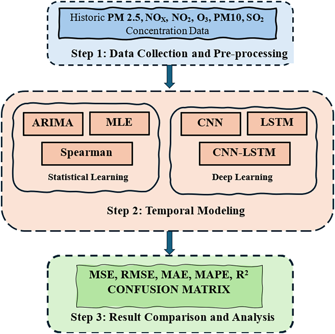
Figure 1: Modeling framework for PM2.5 forecasting using statistical and deep learning approaches, including preprocessing, model training, and evaluation stages

3.1 Data Collection and Preprocessing

This study utilizes historical air quality data comprising (NO2), (NOX), (O3), (PM10) and (SO2) measurements. All Pollutant unit were measured in µg/m3. Daily historical air quality concentration data of TAI PO station in Hong Kong from 01 January 2016, to 31 December 2016 were chosen as the research objects and used as input parameters. The Tai-po is a rural area with less industry and vehicles, making it a better place to live compared to Causeway Bay, Central/Western and Mong-Kok. However, the quality of air is also affected by neighboring areas. The installed sensors record the air pollutant value after each 5 min, and at the end of every hour, these values are averaged. Thus, each day contains 24 averaged values of each pollutant. After collecting 8784 samples/pollutant dataset, the following pre-processing steps were applied:

The missing data were filled using interpolation techniques to maintain continuity of the time series. These values were then normalized using normalization technique. The features were scaled to a range of [0, 1] using min-max normalization for deep learning models. Important air quality parameters were selected based on the Spearman correlation analysis. In addition, feature selection is implemented. At the end, time-series formatting is performed. The data set is structured into sequences for LSTM training, ensuring that temporal dependencies were captured.

3.1.1 Spearman Correlation-Based Feature Selection

To ensure the selection of the most relevant input features for PM2.5 forecasting, Spearman correlation analysis was applied to assess monotonic relationships between PM2.5 concentrations and other pollutant variables such as NO2, NOX, O3, PM10, and SO2. This approach enabled the identification of strongly correlated variables while reducing redundancy in the input space. Variables with low correlation or high multicollinearity were excluded using a combination of Spearman ranking and Variance Inflation Factor (VIF) analysis. This feature selection process improved both model interpretability and training efficiency.

3.1.2 Outlier-Driven Temporal Reassessment

Fig. 2 illustrates a structured decision-making framework designed to enhance the classification accuracy of PM2.5 time series data. The process begins with the input of daily sequences, each comprising 24 hourly PM2.5 observations. An initial model is trained to classify the entire 24 h sequence as a single unit. Subsequently, instances of misclassification identified during training are further examined. Outliers across the complete data space are also detected to understand their potential impact. Each misclassified sequence is then segmented into three equal parts, with each segment containing 8 consecutive observations. This segmentation enables the model to re-evaluate the classification at a finer temporal resolution. If segmentwise classification yields improved predictive accuracy, it is adopted as a more reliable representation of that day. This two-tiered evaluation strategy improves overall model robustness by minimizing the influence of short-lived pollution spikes that might otherwise mislead full-sequence classification.

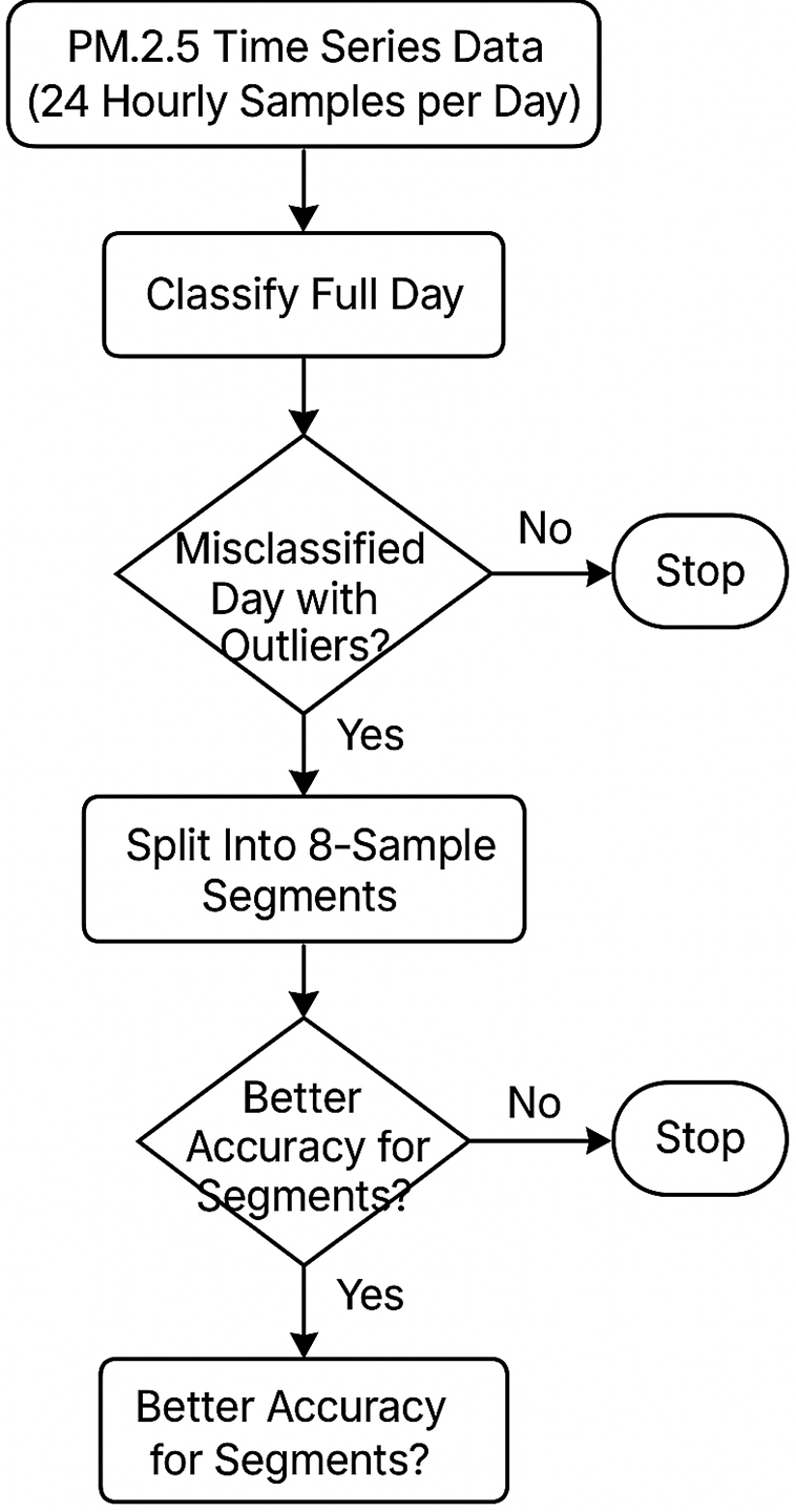
Figure 2: Two-stage decision framework for handling misclassifications caused by outliers through temporal segmentation of PM2.5 sequences

3.2 LSTM-Based PM2.5 Prediction Model

The LSTM model was implemented to capture long-term dependencies in air pollution data. The architecture included:

Input Layer: Sequential air quality data with multiple features. It takes in sequential data where each input sample has time-series features like temperature, humidity, PM2.5 levels, etc.

LSTM Layers: This is the main LSTM layer that captures temporal dependencies in the sequential data. Unlike traditional neural networks, LSTMs have memory cells and gates (input, forget, output) that help retain useful past information while ignoring irrelevant data.

Dropout Layer: To prevent overfitting by randomly disabling 20% of the neurons during training. It ensures that the model does not become too dependent on specific neurons. Moreover, it improves generalization when making predictions on unseen data. If overfitting occurs (high training accuracy but poor validation accuracy), increasing dropout may help.

Dense Output Layer: The purpose of this layer is to map the LSTM output to the final number of required responses. This layer converts the LSTM outputs (which are high-dimensional) into a simpler output space. A fully connected layer with a single neuron for PM2.5 prediction.

Regression Layer: This layer defines the loss function for continuous output values (i.e., for regression tasks). This uses Mean Squared Error (MSE) by default for loss calculation. This layer is ideal for time-series prediction tasks where the output is a continuous numerical value.

Optimizer: Adam optimizer was applied during training.

3.3 CNN-Based Feature Recognition

A CNN model was designed for feature extraction and pattern recognition in pollution datasets. The methodology included:

Data Reshaping: The air quality data was transformed into 2D representations for CNN processing.

Convolutional Layers: Three convolutional layers were applied to extract spatial features from pollution data.

Pooling and Flattening: Max-pooling layers reduced dimensionality, followed by a fully connected layer for classification.

Activation Function: ReLU activation was used in hidden layers, and a Softmax layer was applied for multi-class classification tasks.

3.4 Hybrid CNN-LSTM Model Architecture

To leverage both spatial and temporal dependencies in air quality data, a hybrid deep learning architecture was constructed by integrating Convolutional Neural Networks (CNN) and Long Short-Term Memory (LSTM) layers. The CNN component captures short-range spatial patterns and localized features in pollutant concentrations, while the LSTM layer models long-term temporal dependencies across consecutive hourly readings. This hybrid approach allows the model to learn both localized anomalies and broader temporal trends, resulting in improved prediction performance over standalone CNN or LSTM models.

3.5 ARIMA-Based Statistical Analysis

For baseline comparison, an ARIMA model was used to analyze historical PM2.5 trends and assess predictive accuracy. The implementation involved:

Model Training & Forecasting: The ARIMA model was trained on historical PM2.5 values, and future predictions were generated.

Evaluation Metrics: Model performance was assessed using MAPE, MAE, MSE, and RMSE for comprehensive accuracy measurement.

Regression Model for Prediction: A multiple linear regression model (fitlm) was applied to analyze relationships between PM2.5 and other environmental variables, ensuring predictive robustness.

Time-Series Analysis: Temporal patterns, trends, and seasonal variations in PM2.5 were examined to improve interpretability and forecasting reliability.

Spearman Correlation Analysis: Rank-based correlation coefficients were computed to assess the relationships between PM2.5 and other pollutants.

Correlation Matrix Computation: Pearson and Spearman correlation matrices were generated to evaluate dependencies among key environmental factors, aiding in feature selection and model refinement.

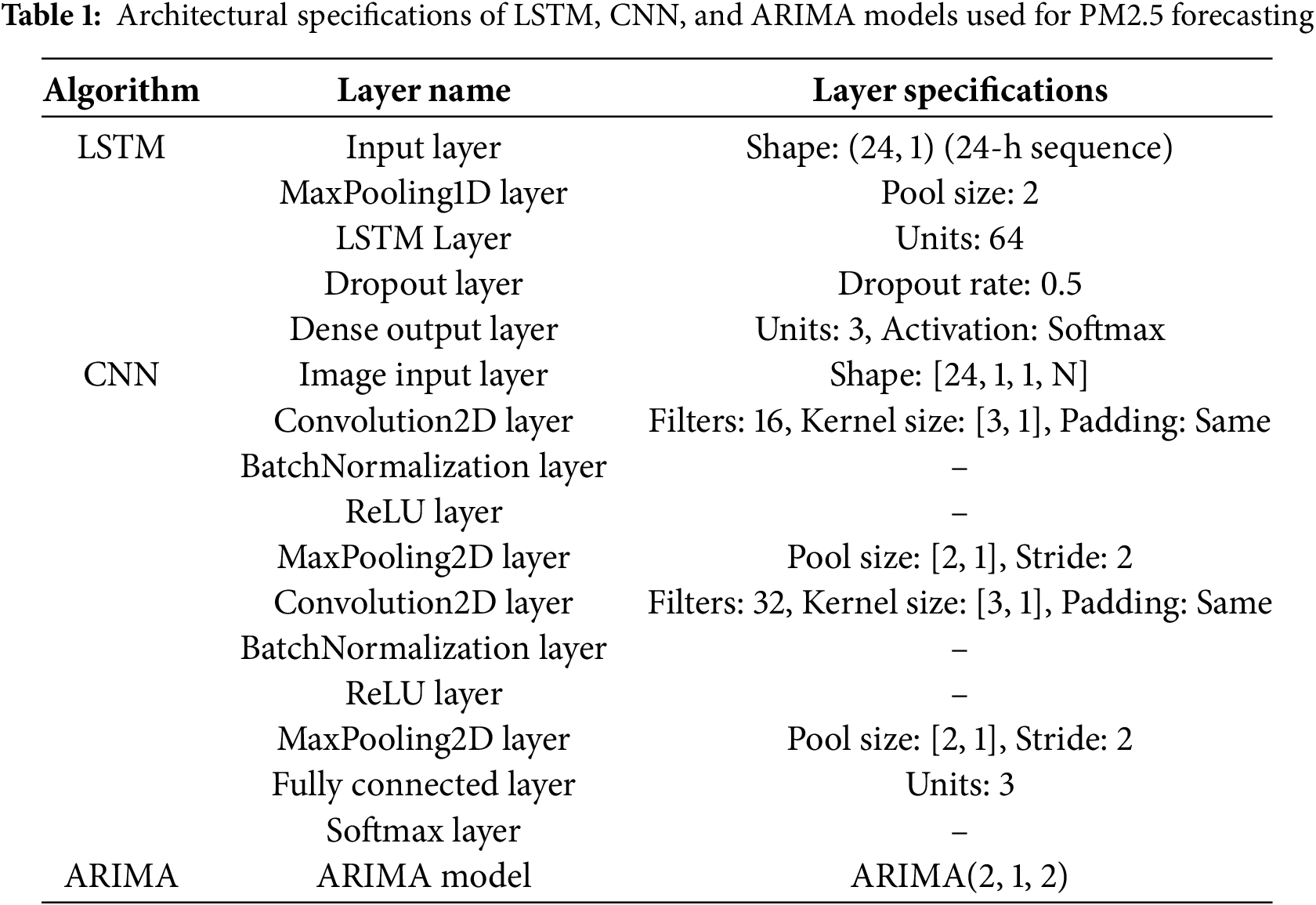
Table 1 explains the layered architecture of all the algorithms used in this study.

3.6 Model Evaluation and Comparison

Let yi∈R denote the observed response value for the ith instance and y^i∈R represent its corresponding model prediction, with n∈N being the cardinality of the dataset. Model performance evaluation employs distinct metrics: regression models (Hybrid CNN-LSTM, LSTM, ARIMA, MLE) are assessed through RMSE, MAE, MAPE, and coefficient of determination (R2), while the CNN architecture is evaluated via classification metrics including confusion matrix analysis, accuracy (Acc), recall (Re), and F1-score.

Mean Absolute Error (MAE): is a regression metric that quantifies the average absolute error between predicted and actual values, disregarding error direction. It is widely used in predictive modeling, such as air quality forecasting, to assess model accuracy.

MAE is widely used in air quality forecasting because it provides a straightforward and interpretable measure of prediction accuracy, offering a clear view of how close the model’s predictions are to the observed values. In air quality prediction, MAE helps assess the reliability of the model in forecasting pollutant concentrations, such as PM2.5 or NO2 levels. A lower MAE indicates better model performance. The formula for MAE is:

MAE=1n∑i=1n|yi−yi^|(1)

Mean Absolute Percentage Error (MAPE): It is a statistical metric used to quantify the accuracy of forecasting or predictive models by measuring the average magnitude of relative prediction errors, expressed as a percentage. It is calculated as:

MAPE=n∑i=1n|yi−y^iyi|×100(2)

Root Mean Squared Error: It is a statistical metric that quantifies the average magnitude of prediction errors in a regression model, calculated as the square root of the mean squared differences between observed and predicted values. RMSE is particularly useful in air quality forecasting because it penalizes large errors more heavily due to the squaring of the residuals, making it sensitive to outliers. This characteristic is important when predicting air quality variables like PM2.5, NO2, or SO2, as large deviations in pollutant concentration can have significant health and environmental implications. A lower RMSE indicates better predictive accuracy, making it an essential tool in assessing the performance of forecasting models in air quality prediction. The formula for RMSE is:

RMSE=1n∑i=1n(yi−yi^)2(3)

Through this methodology, we established a comparative framework for PM2.5 prediction, identifying strengths and weaknesses of deep learning and statistical methods for air pollution prediction.

Mean Squared Error (MSE): It is a statistical metric that quantifies the average squared difference between observed (actual) and predicted values in a regression model. It is often used in regression models to check the accuracy of predictions. It is useful for air quality analysis as it provides a measure of the overall error in predicting pollutant levels, such as PM2.5 or NO2 concentrations. The key characteristic of MSE is that it penalizes larger errors more heavily due to the squaring of the residuals, which is beneficial when large deviations in air pollutant concentrations are critical for health and environmental assessment. Lower MSE values indicate better predictive performance, making it an essential metric to evaluate air quality forecasting models. The formula for MSE is:

MSE=1n∑i=1n(yi−yi^)2(4)

Coefficient of Determination (R2): It measures variance proportion in dependent variable (e.g., pollutant concentration) explained by independent variables in regression. Ranging from 0 to 1, it evaluates model fit, where 0 denotes no explanatory power and 1 indicates perfect prediction of observed data.

In air quality analysis, R2 is a valuable metric for assessing the effectiveness of forecasting models. A higher R2 indicates that the model does a better job of explaining the variability in pollutant levels, such as PM2.5, NO2, or SO2 concentrations. This helps in understanding how well a model can predict future air quality and assess its reliability for decision-making related to air pollution control and public health. However, R2 alone doesn’t guarantee a good model since it doesn’t account for the magnitude of prediction errors, which is why it is often used alongside other metrics like RMSE or MAE.

R2=1−∑i=1n(yi−yi^)2∑i=1n(yi−y¯)2(5)

Confusion Matrix: It evaluates classification performance by comparing predicted labels against true labels. It comprises four key metrics: TP (True positives), TN (True negatives), FP (Type I errors), and FN (Type II errors). This matrix quantifies model errors and correct predictions per class. From these components, several performance metrics can be derived, such as accuracy, precision, recall, and F1 score. In the context of air quality analysis, a confusion matrix is especially useful when classifying air quality levels, such as PM2.5, into categories like Good, Satisfactory, or Poor. For example, the model could be predicting whether air quality falls within a certain range (e.g., PM2.5 levels in the “Moderately Polluted” category), and the confusion matrix helps evaluate how well the model performs in making these predictions. Mathimatically it can be written as

Accuracy=TP+TNTP+TN+FP+FN(6)

Linear Interpolation: is a method used to estimate missing values in a dataset based on the known values. It is commonly used in time-series analysis and other types of data analysis where gaps in the data need to be filled in a meaningful way. There are various types of interpolation methods, such as linear, polynomial, and spline interpolation, with linear interpolation being the most common. In air quality analysis, interpolation can be used to fill in missing air quality measurements (e.g., missing PM2.5 values) in datasets that have gaps due to sensor malfunctions or other issues. By applying interpolation, these missing values can be estimated based on nearby data, ensuring the dataset remains consistent for analysis and modeling. The mathematical form of the formula is

y=y1+(x−x1)(x2−x1)(y2−y1)(7)

This formula estimate the missing value of y at point x based on two known points (x1,y1) and (x2,y2).

4  Results and Discussion

This section presents a comparative performance evaluation between our proposed hybrid deep learning architecture and conventional statistical models. We selected the comparison models based on their relevance in recent literature, performance in prior PM2.5 forecasting studies, and architectural diversity. These include statistical (ARIMA, MLE), tree-based (RF, XGBoost), temporal (LSTM, GRU), hybrid (CNN-LSTM), and spatial-temporal models (Transformer, STN).The historic PM2.5 data is shown in Fig. 3 for the understanding of the trends.

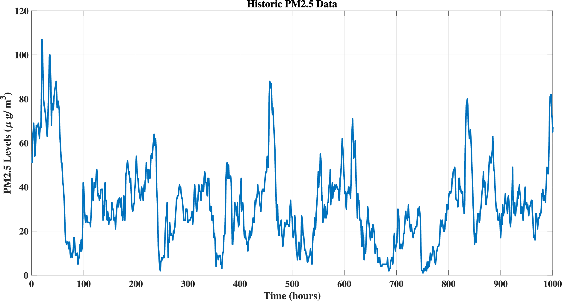
Figure 3: Hourly PM2.5 concentration trend for the year 2016 at Tai Po station, illustrating seasonal and temporal fluctuations

Furthermore, to understand the relationships between PM2.5 with its neighbouring environmental parameters, the correlations are summarized in Table 2.

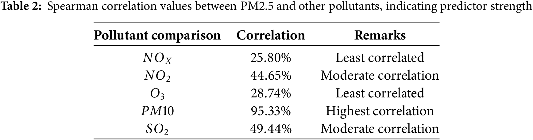
4.1 Analysis Using Spearman Rank Correlation

Spearman’s Rank Correlation was calculated among PM2.5, NO2, NOx, O3, PM10, and SO2 to examine the relationships between these pollutants. As expected, PM2.5 showed a perfect self-correlation (ρ=1.000). A strong positive correlation was observed between PM2.5 and PM10 (ρ≈0.953), indicating that these particulate pollutants often co-occur. Moderate positive correlations were found between PM2.5 and SO2 (ρ≈0.496) as well as NO2 (ρ≈0.450), suggesting that emissions from vehicular and industrial activities significantly influence PM2.5 levels. Comparatively weaker correlations were observed with O3 (ρ≈0.286) and NOx (ρ≈0.261), highlighting the more complex and indirect relationships these gases have with particulate matter concentrations. The complete spearman correlation matrix is shown in Fig. 4. Features with low correlation or high multicollinearity were excluded prior to model training. This filtering step reduced noise and improved model performance.

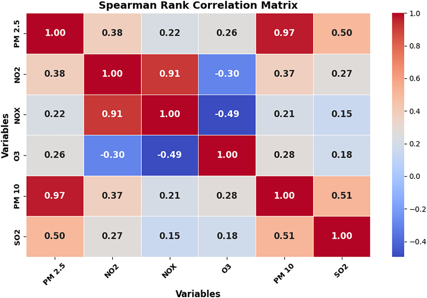
Figure 4: Spearman rank correlation matrix among pollutant variables, highlighting strength and direction of associations with PM2.5

To investigate the temporal trends of key pollutants, Fig. 5 presents the concentrations of PM10 and PM2.5 over time. PM10 is shown as the first line, with PM2.5 overlaid for comparison. The observed fluctuations in both pollutants highlight their changing levels and reveal important patterns across the observation period.

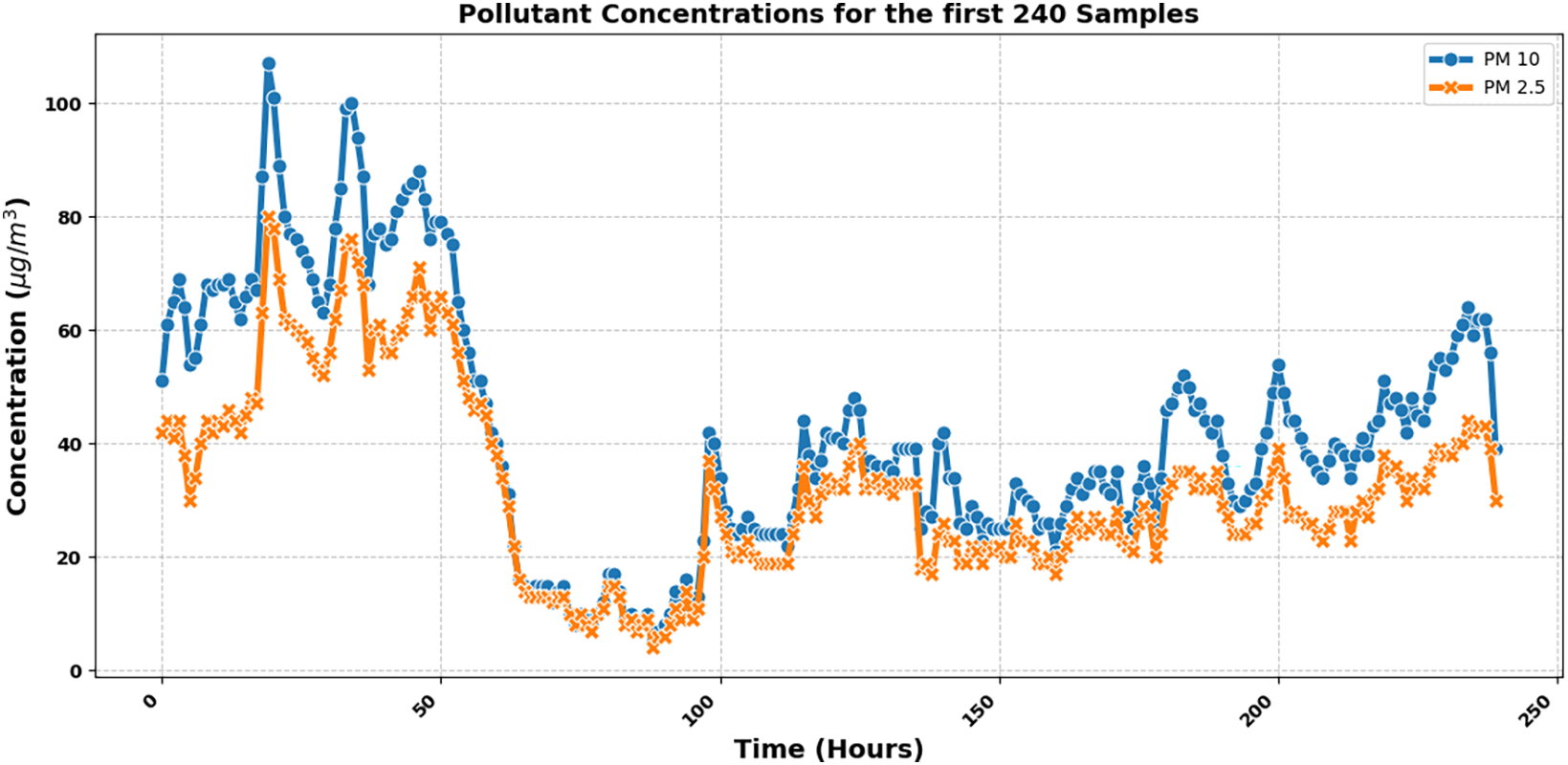
Figure 5: Time-series comparison of PM10 and PM2.5 concentrations showing co-occurring trends and pollutant dynamics

The x-axis represents time in hours, while the y-axis indicates the pollutant concentrations in µg/m3. By visualizing these trends, we can better understand how PM10 and PM2.5 concentrations evolve over the dataset period and assess any potential correlations or patterns between the two pollutants.

Furthermore, a detailed comparative evaluation of multiple models—including the proposed Hybrid CNN-LSTM model, standalone LSTM and CNN models, Maximum Likelihood Estimation (MLE), and ARIMA—has been conducted. The performance of each model was assessed using standard metrics such as RMSE, MAE, MAPE, and R2, and the results are systematically compared and discussed.

4.2 Results of Deep Learning

In this section, standalone LSTM, CNN and their hybrid approach CNN-LSTM will be discussed.

4.2.1 Analysis Using LSTM Model

The LSTM network demonstrated superior performance in capturing temporal dependencies within the time-series data. After training the model on hourly PM2.5 data, which incorporated key environmental features such as O3, SO2, and NO2, the LSTM model achieved an RMSE of 3.75 µg/m3 and an R2 value of 0.9311. This indicates a high level of predictive accuracy, highlighting the model’s ability to estimate PM2.5 concentrations with minimal error.

The LSTM model was particularly effective in capturing daily and weekly fluctuation patterns, making it a reliable tool for short-term air quality forecasting. Its performance is a result of its ability to adapt to non-linear variations in the data, driven by factors such as seasonal changes and traffic-related fluctuations. These aspects of the model allow it to effectively handle the inherent complexities in air quality prediction.

The prediction performance of the LSTM model is depicted in Fig. 6. As shown in the figure, the system successfully predicts PM2.5 levels, demonstrating a strong alignment between the predicted and actual values.

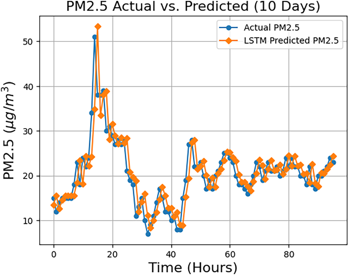
Figure 6: LSTM model’s PM2.5 prediction performance showing alignment between predicted and actual values

The LSTM model consists of a simple yet powerful architecture. It begins with an LSTM layer of 50 units, capturing the temporal dependencies from the input time-series data, which is followed by a Dropout layer to prevent overfitting. The output is passed through a Dense layer with a single neuron, providing the final prediction for PM2.5 concentration. The total number of trainable parameters in the model is 10,451, requiring only 40.82 KB of memory.

4.2.2 Analysis Using CNN Model

To predict air quality based on PM2.5 concentrations, a CNN model was adapted for time-series classification by leveraging 2D convolution layers. Hourly PM2.5 data was reshaped into daily sequences, where each sample represented 24 consecutive hourly values and was formatted as a 4D input of size [24×1×1×N], making it suitable for CNN processing. Daily labels were assigned based on the maximum PM2.5 concentration in each day and categorized into three air quality classes: Good (≤12 µg/m3), Moderate (12–35.4 µg/m3), and Unhealthy (>35.4 µg/m3). The CNN architecture consisted of an input layer followed by two convolutional blocks. Each block included a 2D convolutional layer ([3×1] filter size) with 16 and 32 filters, respectively, batch normalization, ReLU activation, and max pooling ([2×1], stride 2) to progressively extract and condense temporal features from the data. These were followed by a fully connected layer mapping to the three output classes, finalized by a softmax and classification layer.

The CNN is trained using following parameters as shown in Table 3. The trained model achieved an impressive classification accuracy of 97.36%, as evidenced by the confusion matrix. A total of 36 out of 10 days were identified as Good days, yielding an accuracy of 87.80%, while 199 out of 204 days were classified as Moderate days, achieving an accuracy of 97.54%. Additionally, 117 out of 121 Unhealthy days were correctly identified, resulting in an accuracy of 96.70%. These results demonstrate the CNN’s strong capability in detecting temporal pollution patterns and its robustness in accurately classifying air quality levels. Its effectiveness in capturing short-term PM2.5 variations underscores its potential for reliable and timely air quality monitoring. From the Fig. 7, we can see the prediction performance of CNN based model.

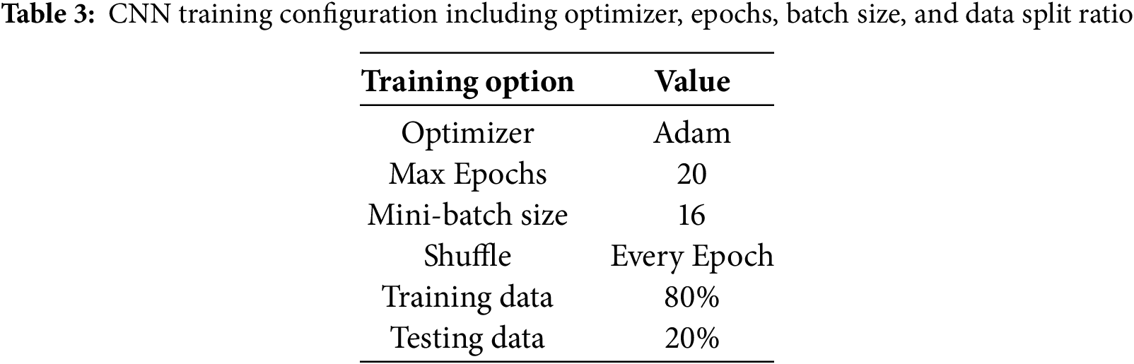
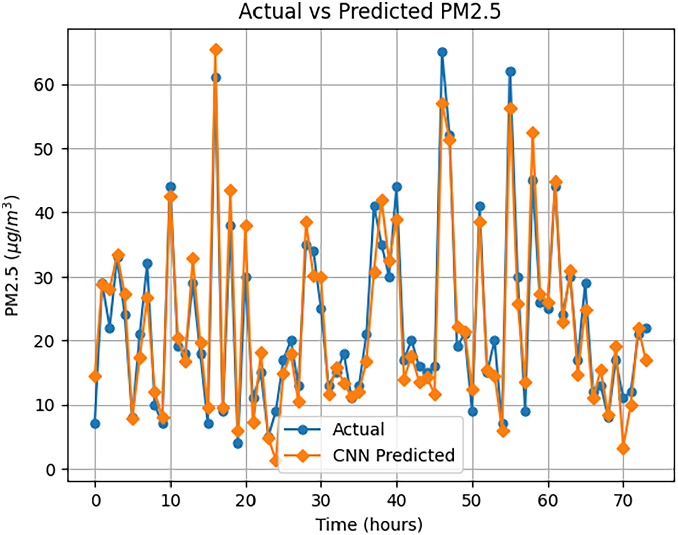
Figure 7: CNN model prediction performance on PM2.5 classification with temporal sequence input

4.2.3 Analysis Using Hybrid CNN-LSTM Model

The proposed CNN-LSTM model architecture begins with a Conv1D layer comprising 64 filters and a kernel size of 3, which is responsible for extracting local temporal features. This layer produces an output shape of (22, 64) and includes 256 trainable parameters. It is followed by a MaxPooling1D layer that reduces the spatial dimensionality to (11, 64), facilitating computational efficiency. The resulting high-level features are then passed to an LSTM layer with 64 units, which captures temporal dependencies and contributes 33,024 trainable parameters. To mitigate the risk of overfitting, a Dropout layer is subsequently applied. Finally, a Dense output layer with 3 neurons performs the classification task, adding 195 trainable parameters. It is important to note that data slicing is introduced in the model to incorporate randomness, which aids in generalization during training.

The performance of the proposed CNN-LSTM model was evaluated using a confusion matrix, revealing insightful classification patterns across the three air quality categories. For the Good class, 10 out of 10 samples (100%) were correctly classified, while none were misclassified as Satisfactory or Unhealthy. In the Satisfactory class, 28 out of 31 samples (90.3%) were correctly identified, while 2 samples were incorrectly classified as Unhealthy and 1 as Good. The Unhealthy category showed similarly strong performance, with 30 out of 32 samples (93.8%) accurately classified, and only 2 samples (6.3%) misclassified as Satisfactory, with no confusion with the Good category. These results suggest that the model is particularly effective in distinguishing Unhealthy air quality, while minor confusion exists between Good and Satisfactory samples, likely due to overlapping feature patterns as visualised in Fig. 8.

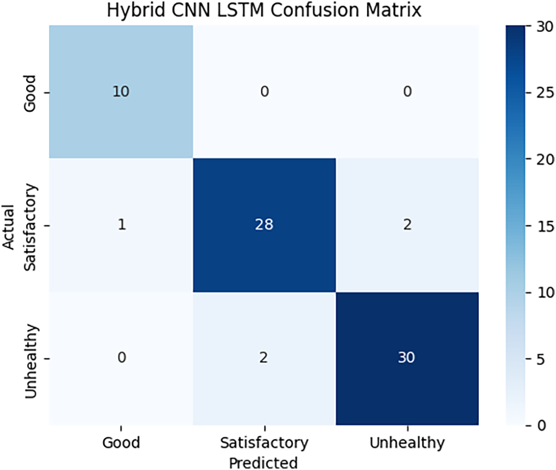
Figure 8: Confusion matrix of the hybrid CNN-LSTM model showing classification accuracy across AQI categories

The proposed CNN-LSTM model achieved a test accuracy of 95% on the dataset, which included 73 days categorized into Good, Satisfactory, and Unhealthy air quality classes. The class-wise performance indicates that the model is highly effective across all categories. For the Unhealthy class, it achieved a precision of 0.94, recall of 0.94, and F1-score of 0.94, indicating strong reliability in detecting hazardous air quality conditions. The Satisfactory class was also well-handled, with a precision of 0.93, recall of 0.90, and F1-score of 0.92, reflecting balanced classification performance. The Good class showed perfect recall at 1.00, meaning all actual Good samples were correctly identified, along with a precision of 0.91 and an F1-score of 0.95, confirming accurate and consistent predictions for this category.

The macro-averaged metrics, which treat all classes equally regardless of support size, resulted in a precision of 0.93, recall of 0.95, and F1-score of 0.94. In contrast, the weighted averages, which take the class distribution into account, yielded precision, recall, and F1-score values of 0.93, reflecting the model’s strong and stable performance even in the presence of slight class imbalance. With a total of 33,475 trainable parameters (130.76 KB) and no non-trainable parameters, the CNN-LSTM architecture proves both lightweight and powerful. These results confirm that the model effectively captures both temporal and spatial dependencies, making it a reliable choice for short-term air quality classification and forecasting. The future PM2.5 value predictions generated by the proposed technique are illustrated in the accompanying Fig. 9, highlighting the model’s capacity to accurately predict temporal trends.

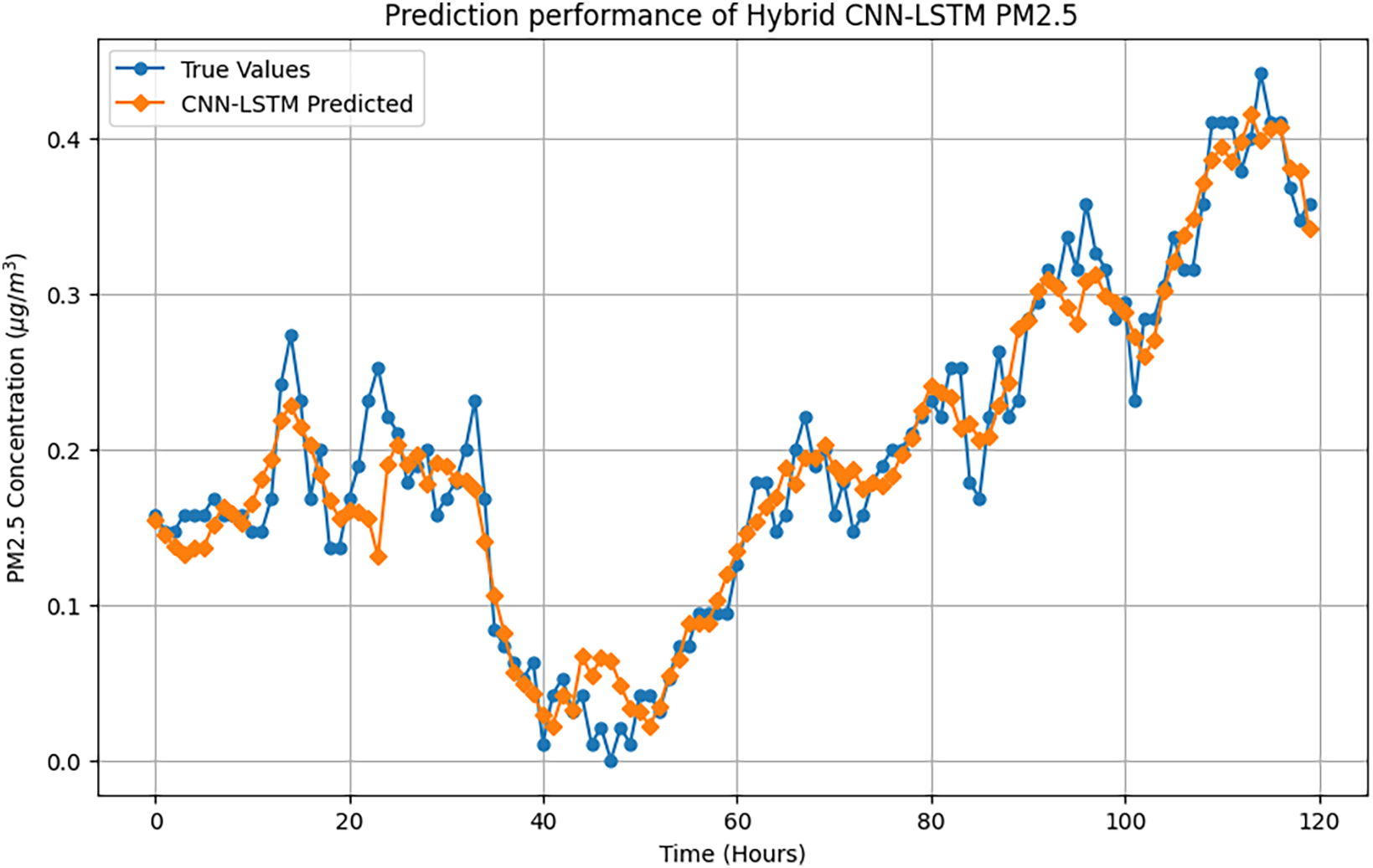
Figure 9: Future PM2.5 concentration prediction using the CNN-LSTM hybrid model

To further evaluate and validate the performance of the proposed CNN-LSTM model, several advanced visual analyzes were performed. Firstly, the Accuracy vs. Loss graph, as shown in Fig. 10, provides a clear overview of the model’s training dynamics, depicting how accuracy steadily increased while loss decreased over training epochs indicating effective learning and convergence.

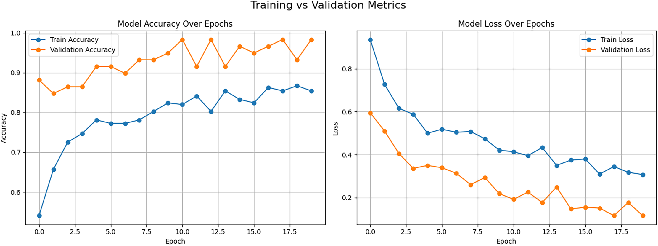
Figure 10: Training performance of CNN-LSTM model showing accuracy and loss curves over epochs

Secondly, multi-class AUC analysis was performed using both macro and micro averaged Precision-Recall (PR) curves, as illustrated in Fig. 11. The analysis clearly demonstrates that the proposed CNN-LSTM model performs exceptionally well across all three air quality categories, with perfect classification for the “Good” class (AUC = 1.00) and very high AUC scores for both “Satisfactory” (0.97) and “Unhealthy” (0.98) categories. The macro-average and micro-average AUC scores, both equal to 0.99, reflect the strong and consistent performance of the model throughout the data set. These results confirm that the model is not only accurate but also reliable in handling different class distributions. This highlights its effectiveness in making accurate predictions even on unseen data, which is critical for practical air quality forecasting applications.

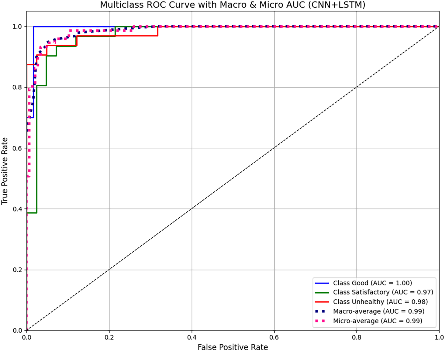
Figure 11: Macro- and micro-averaged AUC-PR curves for multiclass air quality prediction using CNN-LSTM model

Lastly, a misclassified samples visualization was generated, as presented in Fig. 12, showcasing the first ten incorrect predictions made by the model. Initially, each day was treated as a 24-h sequence (i.e., 24 samples per day), which worked well in general but led to certain misclassifications in days containing abrupt pollution spikes. Notably, Day 275 and Day 284 were incorrectly classified due to early-hour or late-hour PM2.5 spikes. For instance, Day 275 exhibited high outlier values such as [64, 67, 62, 60, 59, 45], while Day 284 showed sudden drops after peaking at values like [33, 31, 34, 33, 16, 15, 15, 14].

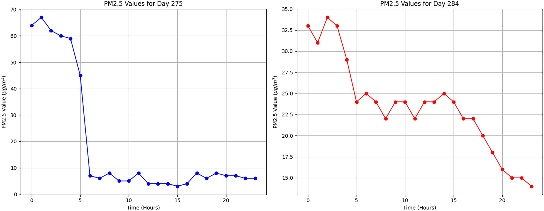
Figure 12: Misclassified hourly PM2.5 sequences for Day 275 (blue) and Day 284 (red) before segmentation, affected by local outliers

To address this issue, a day slicing technique was applied, where each 24-h day was divided into three 8-h segments, allowing for finer-grained classification. This method helped reduce the impact of short-term pollution anomalies that might otherwise dominate the prediction for the entire day. After applying this approach, previously misclassified sequences were correctly labeled, demonstrating that segmentation improves robustness by localizing outlier influence.

Fig. 13 presents the PM2.5 data for the originally misclassified day 275, which contained early hour outliers that skewed the classification. To resolve this issue, the 24-h sequence was divided into three equal 8-h segments. This cutting approach reduced the influence of short-term spikes and resulted in an improved classification. Day 823 was labeled as Unhealthy, while Day 824 and Day 825 were classified as Good.

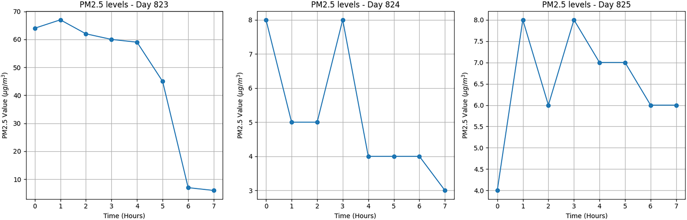
Figure 13: Segmented PM2.5 time series for Day 275, showing correct reclassification after slicing the original day into three 8-hour intervals

Similarly, Fig. 14 shows the PM2.5 values for Day 284, which was initially labeled as Unhealthy based on the full 24-sample sequence. After segmentation, the reclassified portions were assigned as Day 850 (unhealthy), Day 851 (satisfactory) and Day 852 (satisfactory). This adjustment demonstrates how time-based segmentation can effectively mitigate the impact of local outliers and improve the precision of air quality classification. Collectively, these visual and structural enhancements enrich the quantitative findings and offer a deeper understanding of the behavior of the model. In multiple misclassified samples (especially Samples 1 and 4, where Unhealthy was misclassified as Satisfactory), early spikes may have been averaged out due to excessive downsampling (e.g., MaxPooling layers reducing feature maps by 50%), or due to a single Dense layer smoothing out local fluctuations. The revised segmentation strategy effectively mitigates this loss of resolution and strengthens classification fidelity.

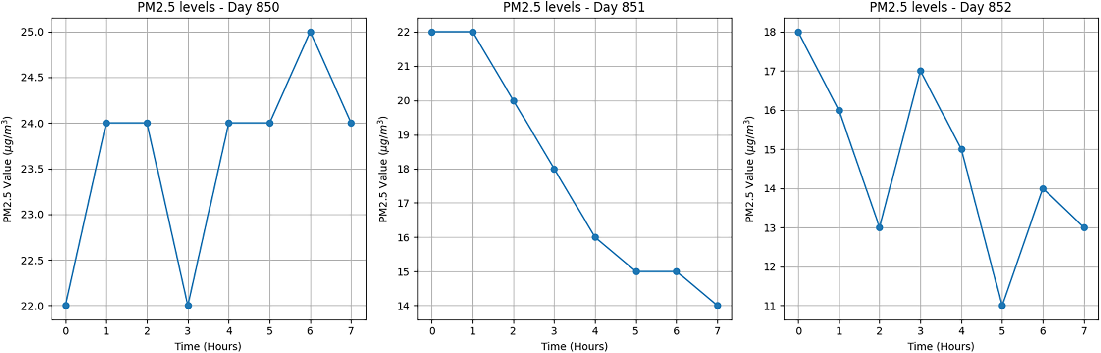
Figure 14: Segmented PM2.5 time series for Day 284, showing improved classification accuracy after splitting the full-day sequence into three segments

4.3 Performance of the Proposed Hybrid Model

The proposed hybrid CNN-LSTM model demonstrated superior performance in PM2.5 prediction tasks compared to both standalone deep learning models and existing benchmarks, as shown in Table 4. It achieved an RMSE of 3.26, MAE of 2.45, MAPE of 9.87%, and an R2 score of 95%. This indicates its strong ability to capture both spatial features via convolutional layers and temporal dependencies through LSTM units.

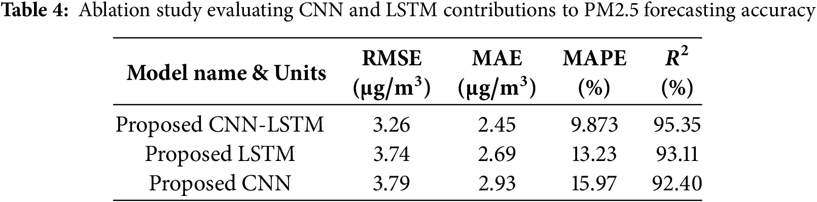
In contrast, the standalone CNN model showed a slightly higher RMSE of 3.79 and MAPE of 15.97%, while the LSTM model resulted in an RMSE of 3.74 and MAPE of 13.23%. These differences underscore the advantage of combining both architectures in a hybrid framework. When compared to previously reported models, the proposed CNN-LSTM significantly outperforms the CNN-LSTM model by Bai et al. [21], which achieved an RMSE of 8.216 and a MAPE of 38.75%. Similar trends were observed for LSTM and CNN models reported in [24,25], all of which reported substantially higher RMSE and MAPE values. These results validate the effectiveness of the hybrid design and its robustness against data irregularities, making it a promising candidate for real-time air quality forecasting applications. The segmentation and reclassification approach successfully corrected initial mispredictions in highly fluctuating periods (e.g., Days 275 and 284), demonstrating the effectiveness of outlier-aware sequence handling. By isolating noisy subsequences and applying CNN-based corrections, the model improved daily classification robustness under extreme pollution variability.

4.4 Ablation Study: Evaluating CNN and LSTM Contributions

To quantify the individual contributions of each component, we conducted an ablation-style evaluation by isolating the CNN and LSTM branches from the hybrid model. Specifically, the CNN only variant removes the recurrent layer, relying solely on spatial feature extraction, while the LSTM-only variant removes convolutional layers and processes raw sequences directly. As shown in the results, the proposed CNN-LSTM model achieves superior performance, compared to the CNN-only and LSTM only variants. This performance gap supports the synergistic benefit of combining CNN’s ability to capture localized spatial patterns with LSTM’s strength in modeling long-term temporal dynamics, thereby validating the hybrid architecture through systematic component analysis. The more insight of the study is presented in Table 4.

4.5 Results of Statistical Model

In this section, the results obtained through ARIMA and MLE will be discussed.

4.5.1 Analysis Using ARIMA Model

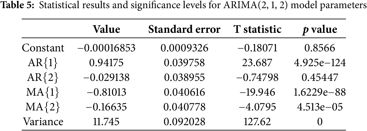
To model the temporal dynamics of PM2.5 concentrations, an ARIMA model was adopted, which includes two autoregressive (AR) terms, one order of differencing (to ensure stationarity), and two moving average (MA) terms. Stationarity is a key prerequisite for ARIMA modeling, and thus a first-order differencing transformation was applied to the original PM2.5 time series to eliminate linear trends and seasonality. This transformation is mathematically represented by:

PM25_diff(t)=PM25(t)−PM25(t−1)(8)

The parameters of the ARIMA(2, 1, 2) model were estimated and the results are summarized in Table 5.

To ensure the stationarity of the PM2.5 time series data, a first-order differencing (d = 1) was applied. Differencing is a standard technique in time series modeling to remove trends and achieve stationarity, which is a necessary condition for ARIMA models. Specifically, the first difference was calculated using the formula:

From the table, it is evident that AR(1) and MA(1) are highly statistically significant, with p-values near zero and large t-statistics (23.687 and −19.946, respectively), indicating their dominant influence on the model’s predictive capability. While the AR(2) term was not statistically significant (p = 0.45447), the MA(2) term was significant with a t-statistic of −4.0795 and a p-value of 4.513e-05. The constant term showed negligible contribution (p = 0.8566), and thus can be considered statistically insignificant. The estimated variance of the model is 11.745 with a high t-statistic of 127.62, further reinforcing model stability.

Furthermore, the performance of the ARIMA(2,1,2) model was evaluated using two standard error metrics. The RMSE was found to be 10.47 µg/m3, suggesting that on average, the model’s predictions deviated from actual PM2.5 values by about 10.47 units. The MAE and MAPE were calculated to be 8.86 µg/m3 and 17.41%, indicating a moderate level of relative prediction error.

Overall, the ARIMA model was least effective in capturing short-term fluctuations and dependencies in PM2.5 concentration data as compared to hybrid CNN-LSTM, LSTM and CNN based models.

4.5.2 Analysis Using Multiple Linear Regression Model

A multiple linear regression (MLR) model was developed to predict PM2.5 concentrations using NO2, NOx, O3, PM10, and SO2 as independent variables. The model can be expressed as:

PM2.5=β0+β1(NO2)+β2(NOx)+β3(O3)+β4(PM10)+β5(SO2)(9)

where β0 represents the intercept and β1 to β5 are the coefficients corresponding to each pollutant. Among the other predictors, NO2 (β1=0.0564) shows a strong positive influence on PM2.5 levels, with a highly significant p-value (ρ≈2.68×10−29). Similarly, for NOx (β2=−0.0127) is negatively associated with PM2.5, and this relationship is statistically significant (ρ≈5.55×10−6). For O3 (coefficient β3=−0.00475) also exhibits a small but significant negative effect (ρ≈0.00128). For PM10 (coefficient β4=0.646) has the largest positive influence, indicating a very strong and direct relationship with PM2.5, and an extremely high significance level (ρ≈0). Furthermore, for SO2 (β5=0.1672) shows a strong positive relationship with PM2.5 concentrations, with a highly significant p-value (ρ≈1.88×10−18). The model is based on 8784 observations, with 8778 degrees of freedom. It achieved a RMSE of 4.06, indicating the average deviation between predicted and actual PM2.5 values. The R2 value is 92.40%, and the adjusted R2 is also 92.40%, meaning that approximately 91.2% of the variability in PM2.5 concentrations is explained by the combined effects of NO2,NOx,O3,PM10, and SO2. The MAE and MAPE are 2.62 µg/m3 and 17.41%, respectively. Additionally, the MLR model’s overall F-statistic is extremely large (F≈1.82×104) with a p-value of 0, confirming that the regression model is statistically significant when compared to a constant model (one without predictors).

Overall, these results suggest that PM10 is the most influential predictor for PM2.5 levels, while NO2 and SO2 also play important roles. NOx and O3 show negative associations, likely reflecting more complex atmospheric processes.

Table 6 presents the performance of traditional statistical models used as baseline benchmarks for PM2.5 forecasting. The ARIMA model achieved an RMSE of 10.47, MAE of 8.86, MAPE of 20.51%, and an R2 value of 75%. While ARIMA is well-suited for capturing linear trends, its limited capacity to model non-linear, multi-variable dynamics contributes to its relatively lower accuracy, particularly for short-term predictions under fluctuating pollution conditions.

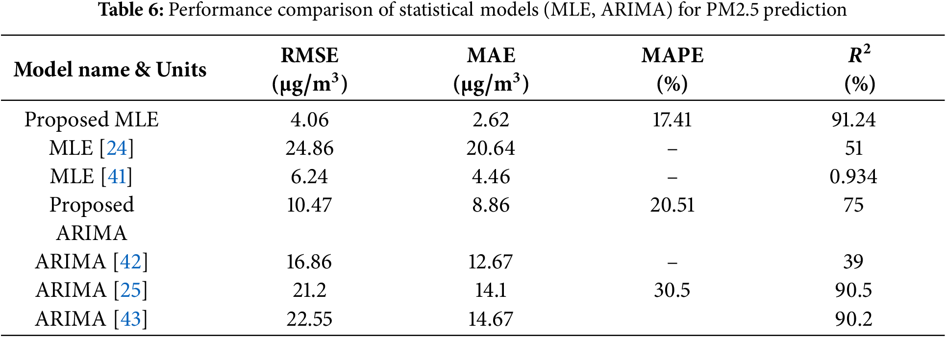
The Multiple Linear Estimation (MLE) model performed slightly better, with an RMSE of 4.06, MAE of 2.62, MAPE of 17.41%, and an R2 of 91.24%. These results reflect MLE’s strength in feature importance interpretation and linear combination modeling, though it still lacks the depth to capture temporal dependencies.

Comparatively, both statistical models underperformed relative to the deep learning and hybrid models. For instance, the proposed CNN-LSTM model reduced the RMSE by over 65% compared to ARIMA and by approximately 20% compared to MLE. These findings highlight the limitations of classical approaches in handling complex pollutant patterns and reinforce the advantage of incorporating deep learning architectures for real-world air quality forecasting.

4.6 Comparison with Relevant Papers

To evaluate the efficacy of the proposed models, we conducted a comparative analysis with recent state-of-the-art approaches including GRU, FBProphet, Transformer, XGBoost, RF and STN. The performance metrics of these models are shown in Table 7. Our proposed CNN-LSTM achieved the lowest RMSE (3.26 µg/m3), MAE (2.45 µg/m3), and MAPE (9.87%), with a strong R2 score of 95%. This outperforms other deep learning models such as GRU (RMSE 8.93) and Transformer (RMSE 19.53), as well as classical methods like FBProphet and ARIMA.

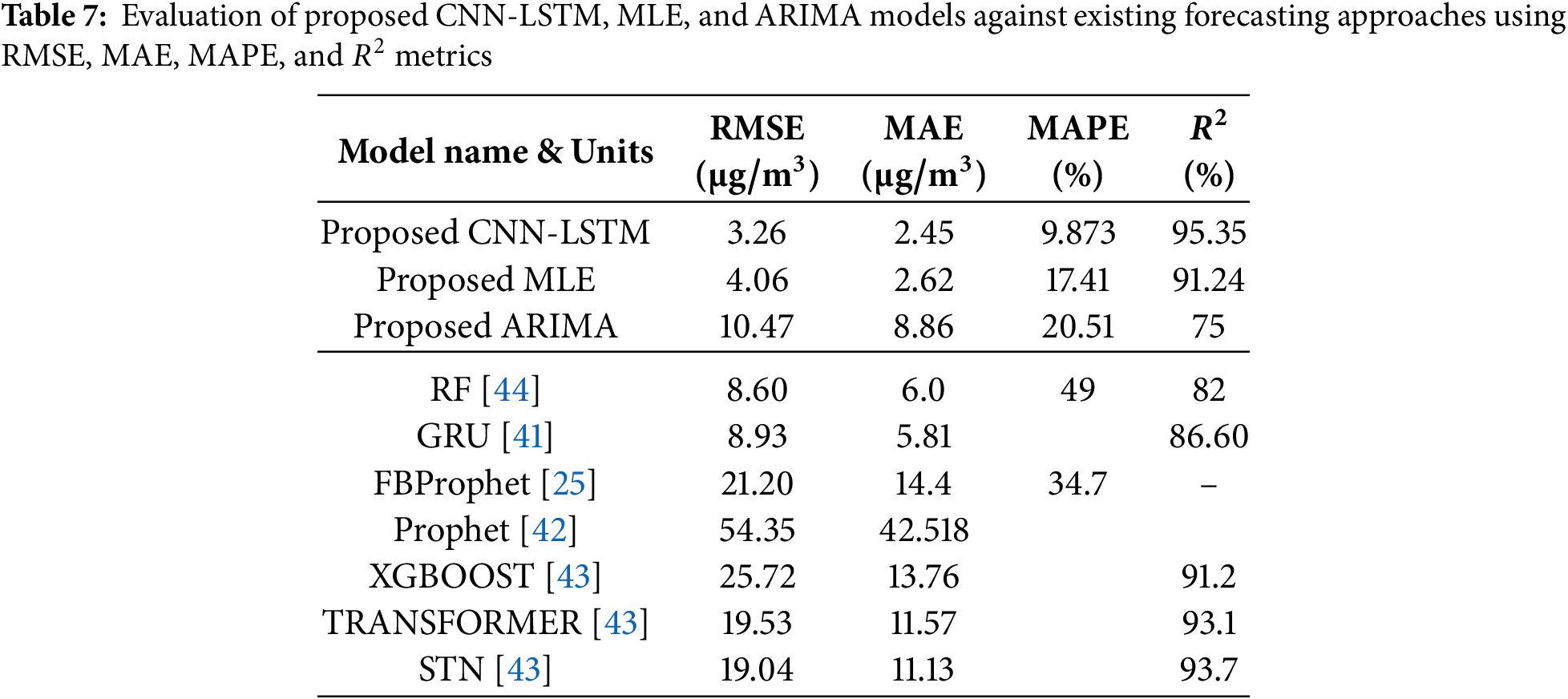
The improvement is attributed to the ability of the hybrid architecture to integrate spatial and temporal features, effectively capturing both short-term fluctuations and long-term dependencies. This comprehensive comparison validates the robustness and generalizability of our model across multiple datasets and methods. Furthermore, the significant performance gap between the proposed CNN-LSTM and single-model architectures highlights the benefit of hybridization in PM2.5 forecasting.

4.7 Benchmarking Against Existing Deep Learning Models

To further validate the effectiveness of the proposed CNN, LSTM, and CNN-LSTM architectures, a comprehensive performance comparison was conducted against existing deep learning models reported in the literature. As shown in Table 8, the proposed hybrid CNN-LSTM model consistently outperforms previously published architectures in terms of RMSE, MAE, MAPE, and R2. Notably, the proposed model achieves an RMSE of 3.26 µg/m3 and an R2 of 95%, which are significantly better than the values reported for other hybrid or standalone deep learning models such as those by Bai et al. [21], Naresh et al. [24], Garg et al. [25], Teng et al. [41] and Zhang et al. [43]. This benchmarking highlights the robustness, generalizability, and predictive strength of the proposed models in PM2.5 forecasting tasks.

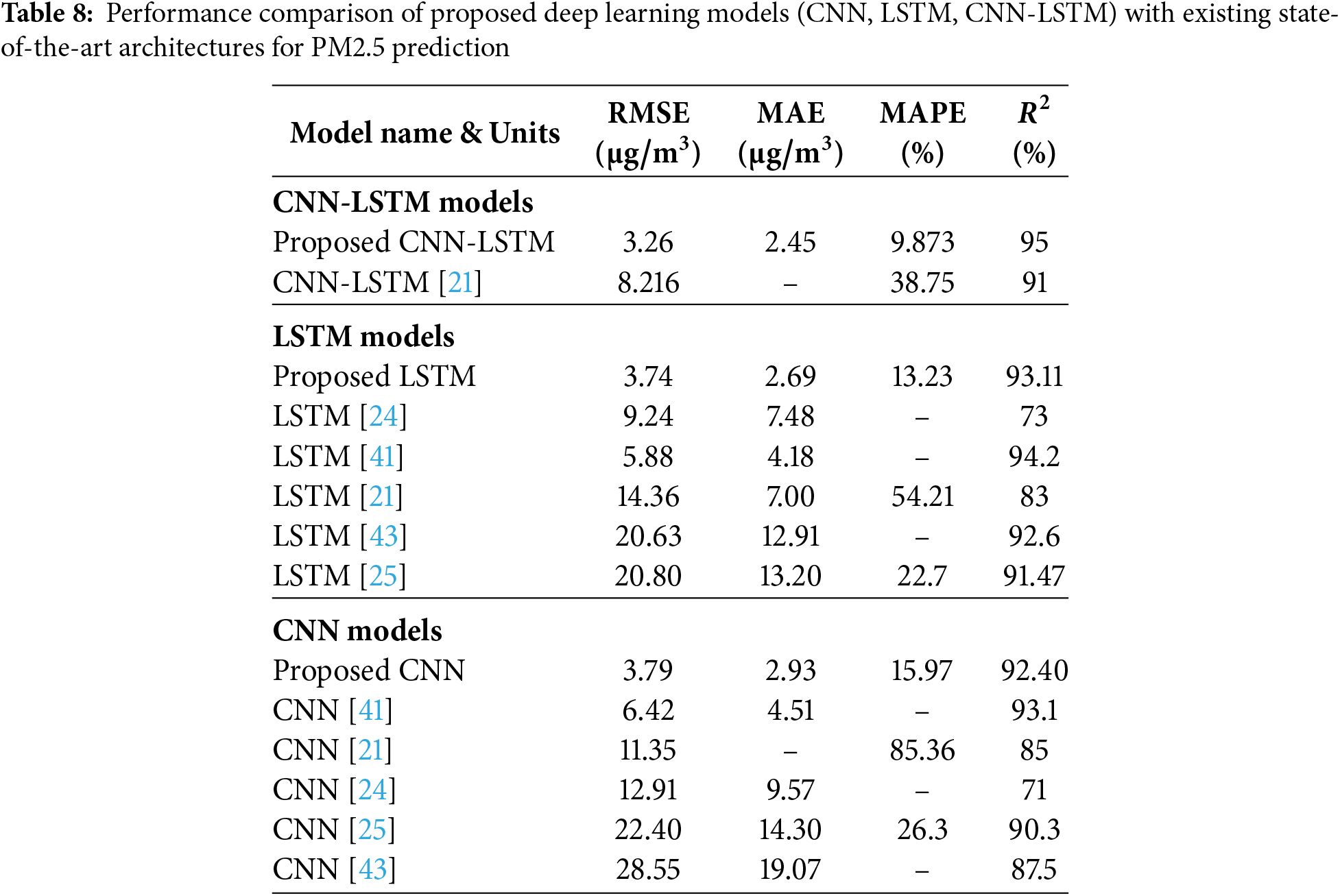
Tables 7 and 8 benchmark the proposed CNN-LSTM model against recent state-of-the-art methods. The superior performance can be attributed to the combination of correlation-driven feature selection, hybrid architecture, and segmentation-based refinement. Compared to CNN-LSTM [21] with RMSE of 8.21 and LSTM [24] with RMSE of 9.24, the proposed approach achieves more than 50% improvement in predictive error.

These empirical results support the effectiveness of each proposed innovation. Spearman-based feature selection reduced redundant inputs, improving generalization. The CNN-LSTM hybrid achieved the best predictive accuracy by learning both spatial patterns and temporal dependencies. Additionally, the segmentation approach corrected misclassified periods and improved robustness in spike-rich pollution days.

4.8 Computational Complexities

In the implemented models, the hybrid CNN-LSTM model has 122,834 trainable parameters, reflecting its higher complexity by combining convolutional feature extraction with temporal sequence modeling. The standalone CNN model, by comparison, has 70,693 trainable parameters, focusing primarily on learning spatial features through convolutional layers. Meanwhile, the standalone LSTM model is the simplest, with 10,451 trainable parameters, dedicated purely to temporal sequence learning. This progressive increase in the number of trainable parameters from LSTM to CNN to CNN-LSTM highlights the added representational power and complexity introduced at each stage.

5  Conclusion

This study presents a comprehensive data-driven framework for PM2.5 air quality forecasting by integrating both deep learning and traditional statistical models. Feature selection was performed using Spearman correlation and multiple linear regression, which identified key pollutant variables including NO2, SO2 and PM10 as strong predictors of PM2.5 concentrations. Among the models evaluated, the proposed hybrid CNN-LSTM architecture consistently outperformed both standalone deep learning models (CNN, LSTM) and traditional statistical baselines (ARIMA, MLE). It achieved an RMSE of 3.26, MAE of 2.45 and R2 of 95%, demonstrating superior predictive accuracy and the ability to effectively capture spatial features and temporal dependencies in complex pollution data. Its robustness was further validated through classification metrics, confusion matrices, and AUC analysis, particularly by distinguishing between the “Good,” “Satisfactory,” and “Unhealthy” AQI categories. In contrast, the ARIMA model exhibited significantly lower performance (RMSE of 10.47, MAPE of 20.51%) due to its linear assumptions and inability to model nonlinear trends. Although the refined MLE regression model performed better (R2 = 91.24%, RMSE = 4.06 µg/m3), it lacked the depth and adaptability offered by deep learning approaches. By combining statistical preprocessing with a hybrid deep learning architecture, our model not only improved forecast accuracy but also enhanced interpretability and resilience to data irregularities (e.g., outlier-driven misclassifications). This cross-domain integration positions the CNN-LSTM model as a highly effective and scalable solution for centralized and real-time air quality monitoring applications.

Despite its strong performance, the proposed framework has certain limitations. The model was trained on data from a specific region, which may limit its generalizability to other geographic or climatic contexts. Real-time responsiveness and deployment feasibility were not evaluated, as the model was evaluated offline without considering latency or computational overhead on resource-limited devices. Furthermore, the absence of external environmental factors, such as temperature or wind speed, and the potential impact of missing or noisy sensor data, may affect robustness in real-world scenarios. Future work will address the limitation of using data from a single station by exploring transfer learning and multistation training for broader applicability. Incorporating meteorological data is expected to boost predictive performance. Furthermore, real-time deployment within the IoT or smart city frameworks is planned to enable timely and automated air quality management.

Acknowledgement: Not applicable.

Funding Statement: The authors received no specific funding for this study.

Author Contributions: The authors confirm contribution to the paper as follows: Conceptualization, Muhammad Fahad Munir, Muhammad Salman Qamar; methodology, Muhammad Salman Qamar; software, Muhammad Fahad Munir; validation, Athar Waseem; formal analysis, Muhammad Fahad Munir; investigation, Muhammad Salman Qamar; resources, Muhammad Fahad Munir, Athar Waseem; data curation, Muhammad Fahad Munir; writing—original draft, Muhammad Salman Qamar; writing—review and editing, Muhammad Salman Qamar, Muhammad Fahad Munir; visualization, Athar Waseem; supervision, Athar Waseem; project administration, Muhammad Salman Qamar. All authors reviewed the results and approved the final version of the manuscript.

Availability of Data and Materials: Due to the nature of this research, the participants did not agree to publicly share their data; therefore, supporting data is not available.

Ethics Approval: Not applicable.

Conflicts of Interest: The authors declare no conflicts of interest to report regarding the present study.

References

1. Xu Z, Niu L, Zhang Z, Hu Q, Zhang D, Huang J, et al. The impacts of land supply on PM2.5 concentration: evidence from 292 cities in China from 2009 to 2017. J Clean Prod. 2022;347(3):131251. doi:10.1016/j.jclepro.2022.131251. [Google Scholar] [CrossRef]

2. Munir MF, Qaman MS, Waseem A, Umar U, Roslee MB, Saleem A. Predicting air quality in pakistan with a focus on smog formation: a machine learning approach. In: 2024 International Conference on Engineering and Emerging Technologies (ICEET); 2024 Dec 27–28; Dubai, United Arab Emirates. p. 1–4. [Google Scholar]

3. Chen H, Guan M, Li H. Air quality prediction based on integrated dual LSTM model. IEEE Access. 2021;9:93285–97. doi:10.1109/access.2021.3093430. [Google Scholar] [CrossRef]

4. Chen F, Zhang W, Mfarrej MFB, Saleem MH, Khan KA, Ma J, et al. Breathing in danger: understanding the multifaceted impact of air pollution on health impacts. Ecotoxicol Environ Saf. 2024;280(60):116532. doi:10.1016/j.ecoenv.2024.116532. [Google Scholar] [PubMed] [CrossRef]

5. He B, Xu HM, Liu HW, Zhang YF. Unique regulatory roles of ncRNAs changed by PM2.5 in human diseases. Ecotoxicol Environ Saf. 2023;255(4):114812. doi:10.1016/j.ecoenv.2023.114812. [Google Scholar] [PubMed] [CrossRef]

6. Fang Z, Kong X, Sensoy A, Cui X, Cheng F. Government’s awareness of environmental protection and corporate green innovation: a natural experiment from the new environmental protection law in China. Econ Anal Policy. 2021;70(1):294–312. doi:10.1016/j.eap.2021.03.003. [Google Scholar] [CrossRef]

7. Chi NNH, Oanh NTK. Photochemical smog modeling of PM2.5 for assessment of associated health impacts in crowded urban area of Southeast Asia. Environ Technol Innovat. 2021;21:101241. doi:10.1016/j.eti.2020.101241. [Google Scholar] [CrossRef]

8. Mushtaq Z, Bangotra P, Gautam AS, Sharma M, Suman, Gautam S, et al. Satellite or ground-based measurements for air pollutants (PM2.5, PM10, SO2, NO2, O3) data and their health hazards: which is most accurate and why? Environ Monit Assess. 2024;196(4):342. doi:10.1007/s10661-024-12462-z. [Google Scholar] [PubMed] [CrossRef]

9. Sun L, Lan Y, Sun X, Liang X, Wang J, Su Y, et al. Deterministic forecasting and probabilistic post-processing of short-term wind speed using statistical methods. J Geophys Res Atmosph. 2024;129(7):e2023JD040134. doi:10.1029/2023jd040134. [Google Scholar] [CrossRef]

10. Tang B, Stanier CO, Carmichael GR, Gao M. Ozone, nitrogen dioxide, and PM2.5 estimation from observation-model machine learning fusion over S. Korea: influence of observation density, chemical transport model resolution, and geostationary remotely sensed AOD. Atmos Environ. 2024;331:120603. doi:10.1016/j.atmosenv.2024.120603. [Google Scholar] [CrossRef]

11. Li Q, Li J, Wang Z, Liu B, Wang W, Wang Z. Development of a city-level surface ozone forecasting system using deep learning techniques and air quality model: application in eastern China. Atmos Environ. 2024;339(12):120865. doi:10.1016/j.atmosenv.2024.120865. [Google Scholar] [CrossRef]

12. Wang H, Qiu J, Liu Y, Fan Q, Lu X, Zhang Y, et al. MEIAT-CMAQ: a modular emission inventory allocation tool for community multiscale air quality model. Atmos Environ. 2024;331:120604. doi:10.1016/j.atmosenv.2024.120604. [Google Scholar] [CrossRef]

13. Karppinen A, Harkonen J, Kukkonen J. A semi-empirical model for evaluating urban participate matter concentrations. WIT Transact Ecol Environ. 2025;37:925–34. [Google Scholar]

14. Xu G, Liu H, Jia C, Zhou T, Shang J, Zhang X, et al. Spatiotemporal patterns and drivers of public concern about air pollution in China: leveraging online big data and interpretable machine learning. Environ Impact Assess Rev. 2025;114(33):107897. doi:10.1016/j.eiar.2025.107897. [Google Scholar] [CrossRef]

15. Abedi A, Baygi MM, Poursafa P, Mehrara M, Amin MM, Hemami F, et al. Air pollution and hospitalization: an autoregressive distributed lag (ARDL) approach. Environ Sci Pollut Res. 2020;27(24):30673–80. doi:10.1007/s11356-020-09152-x. [Google Scholar] [PubMed] [CrossRef]

16. Gao W, Xiao T, Zou L, Li H, Gu S. Analysis and prediction of atmospheric environmental quality based on the autoregressive integrated moving average model (ARIMA Model) in Hunan Province, China. Sustainability. 2024;16(19):8471. doi:10.3390/su16198471. [Google Scholar] [CrossRef]

17. Saravanan D, Kumar KS. IoT based improved air quality index prediction using hybrid FA-ANN-ARMA model. Mat Today Proc. 2022;56(3):1809–19. doi:10.1016/j.matpr.2021.10.474. [Google Scholar] [CrossRef]

18. Yi Y, Guo C, Zheng Y, Chen S, Lin C, Lau AK, et al. Life course associations between ambient fine particulate matter and the prevalence of prediabetes and diabetes: a longitudinal cohort study in Taiwan and Hong Kong. Diabetes Care. 2025;48(1):93–100. doi:10.2337/dc24-1041. [Google Scholar] [PubMed] [CrossRef]

19. Ameer S, Shah MA, Khan A, Song H, Maple C, Islam SU, et al. Comparative analysis of machine learning techniques for predicting air quality in smart cities. IEEE Access. 2019;7:128325–38. doi:10.1109/access.2019.2925082. [Google Scholar] [CrossRef]

20. Zaini N, Ean LW, Ahmed AN, Malek MA. A systematic literature review of deep learning neural network for time series air quality forecasting. Environ Sci Pollut Res Int. 2022;29(4):4958–90. doi:10.1007/s11356-021-17442-1. [Google Scholar] [PubMed] [CrossRef]

21. Bai X, Zhang N, Cao X, Chen W. Prediction of PM2.5 concentration based on a CNN-LSTM neural network algorithm. PeerJ. 2025;12:e17811. doi:10.7717/peerj.17811. [Google Scholar] [PubMed] [CrossRef]

22. Duan J, Gong Y, Luo J, Zhao Z. Air-quality prediction based on the ARIMA-CNN-LSTM combination model optimized by dung beetle optimizer. Sci Rep. 2023;13(1):12127. doi:10.1038/s41598-023-36620-4. [Google Scholar] [PubMed] [CrossRef]

23. He Z, Guo Q. Comparative analysis of multiple deep learning models for forecasting monthly ambient PM2.5 concentrations: a case study in Dezhou City, China. Atmosphere. 2024;15(12):1432. doi:10.3390/atmos15121432. [Google Scholar] [CrossRef]

24. Naresh G, Indira B. Air pollution prediction using multivariate LSTM deep learning model. Int J Intell Syst Appl Eng. 2023;12(8s):211–20. [Google Scholar]

25. Garg S, Jindal H. Evaluation of time series forecasting models for estimation of PM2.5 levels in air. In: 2021 6th International Conference for Convergence in Technology (I2CT); 2021 Apr 2–4; Mumbai, India. p. 1–8. [Google Scholar]

26. Lin J, Zhang Y, Wang K, Xia H, Hua M, Lu K, et al. Long-term impact of PM2.5 exposure on frailty, chronic diseases, and multimorbidity among middle-aged and older adults: insights from a national population-based longitudinal study. Environ Sci Pollut Res. 2024;31(3):4100–10. doi:10.1007/s11356-023-31505-5. [Google Scholar] [PubMed] [CrossRef]

27. Pandey M, Jain V, Godhani N, Tripathi SN, Rai P. Spatio-temporal forecasting of PM2.5 via spatial-diffusion guided encoder-decoder architecture. arXiv:2412.13935. 2024. [Google Scholar]

28. Pan R, Liu T, Ma L. A graph attention recurrent neural network model for PM2.5 prediction: a case study in China from 2015 to 2022. Atmosphere. 2024;15(7):799. doi:10.3390/atmos15070799. [Google Scholar] [CrossRef]

29. Kheder A, Foreback B, Wang L, Liu ZS, Boy M. Deep spatio-temporal neural network for air quality reanalysis. In: Scandinavian Conference on Image Analysis. Cham, Switzerland: Springer; 2025. p. 74–87. [Google Scholar]

30. Ghayoumi Zadeh H, Fayazi A, Rahmani Seryasat O, Rabiee H. A bidirectional long short-term neural network model to predict air pollutant concentrations: a case study of Tehran, Iran. Transact Mach Intell. 2022;5(2):63–76. doi:10.47176/tmi.2022.63. [Google Scholar] [CrossRef]

31. Peng B, Xie B, Wang W, Wu L. Enhancing seasonal PM2.5 estimations in China through Terrain–Wind–Rained Index (TWRIa geographically weighted regression approach. Remote Sens. 2024;16(12):2145. doi:10.3390/rs16122145. [Google Scholar] [CrossRef]

32. Zhang J, Peng Y, Ren B, Li T. PM2.5 concentration prediction based on CNN-BiLSTM and attention mechanism. Algorithms. 2021;14(7):208. doi:10.3390/a14070208. [Google Scholar] [CrossRef]

33. Zhang B, Chen W, Li MZ, Guo X, Zheng Z, Yang R. MGAtt-LSTM: a multi-scale spatial correlation prediction model of PM2.5 concentration based on multi-graph attention. Environ Modell Software. 2024;179(6):106095. doi:10.1016/j.envsoft.2024.106095. [Google Scholar] [CrossRef]

34. Xu J, Wang S, Ying N, Xiao X, Zhang J, Jin Z, et al. Dynamic graph neural network with adaptive edge attributes for air quality prediction: a case study in China. Heliyon. 2023;9(7):e17746. doi:10.1016/j.heliyon.2023.e17746. [Google Scholar] [PubMed] [CrossRef]

35. Koo J-S, Wang K-H, Yun H-Y, Kwon H-Y, Koo Y-S. Development of PM2.5 forecast model combining ConvLSTM and DNN in Seoul. Atmosphere. 2024;15(11):1276. doi:10.3390/atmos15111276. [Google Scholar] [CrossRef]

36. Semmelmann L, Henni S, Weinhardt C. Load forecasting for energy communities: a novel LSTM-XGBoost hybrid model based on smart meter data. Energy Informatics. 2022;5(Suppl 1):24. doi:10.1186/s42162-022-00212-9. [Google Scholar] [CrossRef]

37. Karnati H, Soma A, Alam A, Kalaavathi B. Comprehensive analysis of various imputation and forecasting models for predicting PM2.5 pollutant in Delhi. Neural Comput Applicat. 2025;37(17):11441–58. doi:10.1007/s00521-025-11047-2. [Google Scholar] [CrossRef]

38. Gun AR, Dokur E, Yuzgec U, Kurban M. Short-term solar power forecasting based on CEEMDAN and kernel extreme learning machine. Elektron Elektrotech. 2023;29(2):28–34. doi:10.5755/j02.eie.33856. [Google Scholar] [CrossRef]

39. Wang S, Huang Z, Ji H, Zhao H, Zhou G, Sun X. PM2.5 hourly concentration prediction based on graph capsule networks. Electron Res Arch. 2023;31(1):509–29. doi:10.3934/era.2023025. [Google Scholar] [CrossRef]

40. Zhao G, Yang X, Shi J, He H, Wang Q. A PM2.5 spatiotemporal prediction model based on mixed graph convolutional GRU and self-attention network. Environ Pollut. 2025;368(5):125748. doi:10.1016/j.envpol.2025.125748. [Google Scholar] [PubMed] [CrossRef]

41. Teng M, Li S, Xing J, Song G, Yang J, Dong J, et al. 24-hour prediction of PM2.5 concentrations by combining empirical mode decomposition and bidirectional long short-term memory neural network. Sci Total Environt. 2022;821:153276. doi:10.1016/j.scitotenv.2022.153276. [Google Scholar] [PubMed] [CrossRef]

42. Ansari M, Alam M. An intelligent IoT-cloud-based air pollution forecasting model using univariate time-series analysis. Arab J Sci Eng. 2024;49(3):3135–62. doi:10.1007/s13369-023-07876-9. [Google Scholar] [PubMed] [CrossRef]

43. Zhang Z, Zhang S. Modeling air quality PM2.5 forecasting using deep sparse attention-based transformer networks. Int J Environ Sci Technol. 2023;20(12):13535–50. doi:10.1007/s13762-023-04900-1. [Google Scholar] [CrossRef]

44. Gündoğdu S, Elbir T. A data-driven approach for PM2.5 estimation in a metropolis: random forest modeling based on ERA5 reanalysis data. Environ Res Communicat. 2024;6(3):035029. doi:10.1088/2515-7620/ad352d. [Google Scholar] [CrossRef]