Radial Basis Function Neural Network Adaptive Controller for Wearable Upper-Limb Exoskeleton with Disturbance Observer

1  Introduction

Motor function impairments frequently stem from neurological conditions such as spinal cord injuries and strokes [1–3]. In the rehabilitation context, designing appropriate exercises plays a crucial role in helping patients regain motor functions necessary for daily activities [4,5]. However, traditional rehabilitation methods heavily rely on one-on-one manual treatment provided by physiotherapists, who subjectively determine exercise difficulty levels and adaptations based on their expertise [6]. This labor-intensive approach highlights the challenges posed by the subjective nature of therapist perception [7]. Consequently, there is a growing interest in robotic-assisted devices as they have the potential to alleviate muscle atrophy in patients and reduce the physical demands placed on physiotherapists [8]. In addition, those devices can ensure a certain level of rehabilitation automation highly required for special types of disabilities.

Robot-assisted systems which involve a high level of interaction between the device and the patient, have become a significant area of interest in robotics, particularly in the context of rehabilitating patients with neurological disabilities [9–11]. Exoskeleton robots have been utilized in the implementation of rehabilitation programs to support physiotherapists and individuals recovering from post-stroke impairments.

The control strategies employed in rehabilitation robots are essential for achieving optimal performance in various rehabilitation treatments [12–14]. Zhao et al. [15] investigated a back stepping controller based on extended state observer for a hydraulic driven lower limb exoskeleton robot to enhance the functionality of load-bearing capacity and to reduce fatigue. Zhang et al. [16] proposed an estimated time-delay approach using Neural Network (NN) of a model-free proportional-derivative controller for a lower-limb exoskeleton. They validated the efficiency of their control system using a simulated model of an lower-limb exoskeleton. Yang et al. [17] proposed an NN controller for a lower-limb exoskeleton robot to conduct trajectory tracking tasks to compensate for external disturbances and unknown parameters. They validated their control system through simulation in MATLAB. Al-dujaili et al. [18] presented an active disturbance rejection control scheme for knee-joint motion control in an exoskeleton medical robot, utilizing both linear and nonlinear extended state observers for disturbance estimation. Asl et al. [19] also developed an NN feedback trajectory tracking controller for a robotic exoskeleton to compensate the nonlinear dynamics of the exoskeleton. Wu et al. [20] proposed a novel control strategy combining Sliding Mode Controller (SMC) and dynamic movement primitives for a reconfigurable upper-limb rehabilitation exoskeleton. Through experimental validation, they demonstrated that sliding mode control under a combinational reaching law outperforms traditional methods such as Proportional-Integral-Derivative (PID) and power reaching law-based sliding mode control in trajectory tracking. Alwand et al. [21] introduced a hybrid control strategy combining active disturbance rejection control and SMC to enhance the tracking performance of a lower limb exoskeleton for hip and knee rehabilitation. Simulation results demonstrated that their controller outperformed conventional approaches by achieving faster tracking, improved disturbance rejection, reduced chattering, and lower control effort. Motivated by the reliable estimation ability of the NN, this work proposed a NN estimation method to determine the unknown parameters.

Table 1 provides a comparative analysis of several existing studies that have developed controller methods for various applications. The focus of the studies, shown in Table 1, was on the control methods, the application as well as the study highlights including advantages and challenges of those studies. By examining Table 1, it can be observed that the surveyed works were relatively new, ranging from 2018 to 2024. In addition, those studies were concerned with the upper-limb and lower-limb as they were the most common motor disabilities. Challenges such as stability, robustness, uncertainties and disturbances were tackled with different levels of accuracy. In Table 1, controller methods are given by: Finite-time Fractional-order Nonsingular Fast Terminal Sliding Mode Control (FONFTSMC), Neural-Fuzzy Adaptive Controller (NFAC), Model-Free based Neural Network Control with Time-Delay Estimation (TDE-MFNNC), Repetitive Learning Control (RLC), Non-singular Fast Terminal Sliding Mode Control method based on Nonlinear Disturbance Observer (NFTSMC-NDO), Iterative Learning Control (ILC), Fractional-Order Ultra-local Model-based NN Sliding Mode Controller (FO-NNSMC), Adaptive Fuzzy Control (AFC) and Robust Adaptive Radial Basis Function Neural Network (RABFNN) have been used.

From the literature presented in Table 1, the researchers have investigated several controller strategies to increase the tracking performance under external disturbances. Although prior controllers in Table 1 have contributed significantly to the field of rehabilitation robotics, several critical limitations persist. In terms of disturbance handling, some approaches lack explicit disturbance observers, making them less robust against unpredictable human-robot interaction forces. Others rely on the assumption of constant disturbances, which reduces their effectiveness under dynamic patient movements. Regarding stability guarantees, certain methods require prior knowledge of disturbance bounds while others adopt overly conservative designs that compromise responsiveness. Clinical adaptability is also a concern, as some controllers require manual tuning for different rehabilitation modes, and others fail to adjust to a patient’s recovery progression over time. These limitations point to the need for a more adaptive, robust, and clinically scalable control strategy.

Motivated by the weakness of the existing works in Table 1, the novelty of this paper lies in the combination of an adaptive controller, Radial Basis Function Neural Network (RBFNN), and disturbance observer to enhance control performance as well as address unknown disturbances and uncertainties in a wearable assistive upper-limb exoskeleton. More explicitly, our paper presented the following contributions:

•   An adaptive neural network controller was established based on a high-dimensional integral-type Lyapunov function and associated stability strategies. This design allowed the tracking error to remain within a prescribed boundary while ensuring efficient trajectory tracking.

•   A RBFNN was developed to estimate the uncertain parameters of the nonlinear dynamic model. This enhanced the controller’s adaptability and improved overall system performance under varying conditions.

•   A disturbance observer was integrated into the control framework to compensate for unknown external disturbances. Its implementation increased the robustness of the controller and enabled accurate trajectory tracking in dynamic environments.

These contributions collectively strengthened the capabilities of the adaptive neural network control system, enabling more effective and reliable performance for upper-limb exoskeleton application.

The remainder of this article has been structured as follows: In Section 2, the structure of the upper-limb exoskeleton and the dynamic model have been given. Section 3 addresses the adaptive neural network controller development. Section 4 represents validation of the adaptive neural network controller on an upper-limb exoskeleton prototype. Section 5 concludes this paper.

2  Structure of Upper-Limb Exoskeleton System

The main purpose of upper-limb exoskeleton is to aid patients with muscle injuries in improving their motor capabilities for daily activities. In this section, we have presented a comprehensive overview of the mechanical design and dynamics of the prototype exoskeleton.

2.1 Mechanical Design and Structure

In this study, an upper-limb exoskeleton, which comprised four Degrees of Freedoms (DOFs) that represents four active joints, was considered. Specifically, the shoulder had two DOFs for abduction/adduction and flexion/extension. The elbow had one DOF for flexion/extension, and the wrist had one DOF for ulnar/radial deviation. Fig. 1 shows the Geometric representation of upper-limb exoskeleton.

Figure 1: Geometric representation of upper-limb exoskeleton

To simplify notation, the abbreviations SP, SR, EP, and WY have been used to represent shoulder pitch, shoulder roll, elbow pitch, and wrist yaw, respectively.

2.2 Dynamic Model of Upper-Limb Exoskeleton

In the present study, the upper-limb exoskeleton dynamic model is considered as follows:

ℳ(q)q¨+𝒞(q,q˙)+𝒢(q)+ℱext(t)=τc+τh(1)

where ℳ(q)∈Rn×n represents the mass-inertia matrix, and n is the number of joints. The vector q∈Rn denotes the joint coordinates. 𝒞(q,q˙)∈Rn represents the Coriolis and centrifugal force effects. The vector 𝒢(q)∈Rn accounts for gravitational forces. ℱext(t)∈Rn denotes external disturbances. τc∈Rn is the applied control torque, and τh represents the interaction forces between the human and the exoskeleton. The inertia matrix ℳ(q), which captures the distribution of mass and rotational inertia of the links with respect to the joints is represented as follows:

ℳ(q)=[ℳ11(q)ℳ12(q)⋯ℳ1n(q)ℳ21(q)ℳ22(q)⋯ℳ2n(q)⋮⋮⋱⋮ℳn1(q)ℳn2(q)⋯ℳnn(q)](2)

The centripetal and Coriolis matrix C(q,q˙) is represented as follows:

C(q,q˙)=[𝒞11(q)𝒞12(q)⋯𝒞1n(q)𝒞21(q)𝒞22(q)⋯𝒞2n(q)⋮⋮⋱⋮𝒞n1(q)𝒞n2(q)⋯𝒞nn(q)](3)

where 𝒞ij is the element of 𝒞(q,q˙) given as follows:

𝒞ij=∑k=1n12(∂ℳij∂qk+∂ℳik∂qj−∂ℳjk∂qi)q˙k(4)

The gravitational forces vector 𝒢(q) is defined as:

𝒢(q)=[𝒢1(q)𝒢2(q)⋮𝒢n(q)](5)

Each element 𝒢i(q) represents the gravitational forces acting on the i-th joint due to the weight of the links distal to and including link i. It is computed from the potential energy of the system and typically depends on the configuration q of the manipulator.

To obtain the state equations, we define the state vector as x=[x1x2]T, where

{x1=qx2=x˙1=q˙(6)

If we substitute Eq. (6) into Eq. (1), we obtain the state equation, given as follows:

{x˙1=x2x˙2=ℳ−1(q)[−𝒞(q,q˙)x2−𝒢(q)−ℱext(t)+τc+τh](7)

The mass-inertia matrix, denoted as ℳ(q), can be break down into two parts: the known matrix ℳk(q) and the unknown matrix Δℳ, as shown below:

ℳ(q)=ℳk(q)+Δℳ(8)

where Δℳ∈Rn×n is the inertia matrix that contains unknown parameters, while ℳk(q) represents a diagonal matrix with non-zero elements (ℳkii(q)≠0).

By substituting Eq. (7) into Eq. (8), we obtain:

ℳk(q)x˙2=ℋ(x)+𝒬+τc(9)

In Eq. (9), 𝒬=[(I+ℳk(q)Δℳ−1)(τh−ℱext(t))+ℳk(q)Δℳ−1τc]∈Rn represents disturbance elements, while ℋ(x)=[(I+ℳk(q)Δℳ−1)(−𝒢(q)−𝒞(q,q˙)x2)]∈Rn denotes unknown and uncertain parameters. It highlights the presence of both disturbance elements and unknown and uncertain parameters within the system dynamics.

Lemma 1: Consider a continuous and differentiable function Ψ(t) [28]:

γ1≤‖Ψ(t)‖≤γ2,∀t∈[t0,t1](10)

where γ1 and γ2 are positive constant values. Then, its derivative Ψ˙(t) is bounded.

Assumption 1: The external force ℱext(t)∈Rn is limited by a positive constant δ as described in [17]. Therefore, we have:

‖ℱext(t)‖<δ(11)

where δ represents a positive constant.

Assumption 2: We assume that 𝒬:R+⟶Rn and 𝒬˙ are symmetric matrices and bounded:

‖𝒬‖≤λ,‖𝒬˙‖≤μ,∀t∈R+(12)

where λ and μ are positive constant values.

Remark 1: Referring to Eq. (9), 𝒬 is expressed as follows:

𝒬=(I+ℳk−1(q))τh−(I+ℳk−1(q))ℱext(t)+ℳk(q)Δℳ−1τc(13)

In many robotic systems, the actuator inputs are subject to saturation constraints, which impose a bounded condition on the control system output τc. Consequently, ℳk(q)Δℳ−1τc remains bounded. Similarly, in the term (I+ℳk−1(q))ℱext(t), where ℱext(t) represents external forces, it is bounded based on Assumption 1. Therefore, (I+ℳk−1(q))ℱext(t) is also bounded. The variable τh represents the forces between the human and the exoskeleton, which is bounded according to [29]. Hence, (I+ℳk−1(q))τh is bounded as well. Consequently, the variable 𝒬 satisfies Assumption 2 by being bounded.

3  Adaptive Neural Network Controller and Stability Analysis

This study presents an adaptive neural network controller using a high-dimensional integral-type Lyapunov function for a wearable assistive upper-limb exoskeleton. The objective of the adaptive controller is the integration between Lyapunov function, RBFNN estimator, and disturbance observer for increasing robustness and consider unknown disturbances and uncertainties. This section presents the development of the adaptive neural network controller along with its stability analysis. Fig. 2 shows the logic diagram of the proposed adaptive neural network controller.

Figure 2: The logic diagram of the controller

The tracking error is defined as:

e=q−qd(14)

where qd represents the desired trajectory and q is the actual trajectory. The tracking error z of the control system is given by:

z=Λe+e˙(15)

Here, Λ=diag[λ1,λ2,…,λ3] is a positive definite symmetric matrix. According to Eq. (15), several linear differential functions can be defined to ensure that e converges when z=0. Consequently, e˙→0 as t→∞. By differentiating Eq. (15), we obtain:

z˙=Λe˙+e¨=Λe˙+q¨−q¨d(16)

By substituting Eq. (9) into Eq. (16), the following Eq. (17) is obtained:

z˙=Mk−1(ℋ(x)+𝒬+τc)+v(17)

where v=[v1,v2,…,vn]T and z=[z1,z2,…,zn]T. The elements of v are defined as:

vi=λie˙i−q¨d(18)

where ei is the elements of tracking error, ei(i=1,2,…,n). An efficient controller can ensure actual trajectory tracks the desired trajectory and guarantees system stability in the presence of unknown disturbances. To achieve this, the controller’s output, τc, is designed to converge to zero, i.e., z⟶0 [27,30].

3.1 Radial Basis Function Neural Network Estimator

In this paper, the RBFNN estimator has been used to estimate the uncertainties parameters. The RBFNN is one type of artificial NN that uses radial basis functions as activation functions which is particularly effective for function approximation, pattern recognition, and nonlinear system estimation. When applied as an estimator, the RBFNN is used to model and predict outputs from given inputs, especially when the system being modeled is complex or nonlinear. In Eq. (9), ℋ∈Rn represents an uncertainty term and the RBFNN estimator has been utilized to estimate the uncertain term [31].

Lemma 2: The universal approximation theorem states that any continuous function can be approximated with arbitrary precision using a linearly parameterized estimator [32]. Mathematically, it can be represented as:

F(Γ)=ψTν(Γ)+ε(19)

where F(Γ):Rn⟶R is the continuous function, Γ∈Rm represents the input vector, ψ∈Rl denotes the adjustable weight vector, ν(Γ) represents a continuous function, and ε(Γ) is a bounded estimation error.

The bounded estimation error ε(Γ) in Eq. (19) satisfies the condition:

|ε(Γ)|≤ε¯,∀Γ∈ΩΓ(20)

Here, ε¯ represents a positive constant number (ε¯>0), and ΩΓ denotes the domain of the input vector Γ. This inequality ensures the estimation error remains within a certain bound for all valid values of Γ. By considering ω∗ as the optimal constant weight, Eq. (19) can be rewritten as:

F(Γ)=ω∗TΦ(Γ)+ϱ(21)

Here, Φ(Γ)=diag[Φ1(Γ),Φ2(Γ),…,Φn(Γ)]T represents the Gaussian function, which is defined as:

Φi=exp⁡[−(Γ−ci)T(Γ−ci)σi2],i=1,2,…,n(22)

In the above equation, ci=[c1,c2,…,ci] represents the receptive field center, and σi is the Gaussian function width. Additionally, there exists a positive constant β such that |Φ(Γ)|≤β with β>0. ϱ represents the smallest possible estimation error of the RBFNN. From the estimation capability of RBFNN, it is known that the estimation error is bounded by the constant ϱ∗, i.e., |ϱ|≤ϱ∗, where ϱ∗ is a positive constant. Therefore, the estimation of the uncertain term ℋ(x) in Eq. (9) using the RBFNN can be expressed as:

ℋ(x)=−ω∗TΦ(x)−ϵ(23)

Here, ω∗T=diag[ωi], i=1,2,…,n is the RBFNN optimal weight, ℋ is the hidden-layer output, and ϵ is a bounded estimated error. We can infer from Eq. (9) that ℋ(x) as represents an unknown uncertain term that can be estimated by the RBFNN.

Since the exoskeleton has 4 DOFs, the number of neurons in the output layer is set to 4. The number of input variables is also chosen as 4, corresponding to the system’s states. The hidden layer is configured with 128 neurons. It is worth noting that, due to the continuity of ℋ and based on Lemma 1 and Eq. (19), the function is bounded. However, it does not depend on the bounded estimation error ϵ. Fig. 3 architecture of the RBFNN to estimate ℋ.

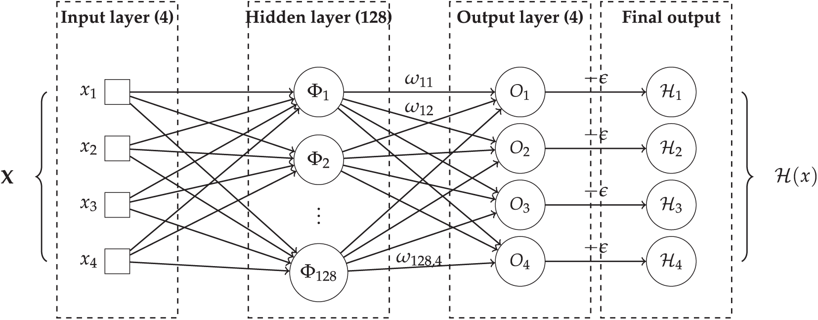
Figure 3: Architecture of the RBFNN with 4 inputs, 128 hidden neurons (Φ), and 4 outputs (H), where O=−ω∗TΦ(x)

3.2 Controller Development with Disturbance Observer

The stability and robustness of the adaptive neural network controller are analyzed by the Lyapunov functions. A candidate Lyapunov function is defined as follows [33]:

V1=zTSz(24)

where S is given as follows:

S=diag[∫01ℳk11(x¯,θz1+ν1)α11dθ...∫01ℳknn(x¯,θzn+νn)αnndθ](25)

For the system stability proof, we define the equation:

Aθ=∫01θAαdθ(26)

Here, Aα=diag[Aα11,Aα22,...,Aαnn], and we make the assumption:

Aαii(x¯,θz1+νi)=Mkii(x¯,θz1+νi)αii(27)

Here, αii=diag[α11,α22,...,αnn] is a positive definite diagonal matrix of size n×n, and x¯=x1. For simplicity, we assume that α11=α22=...=αnn. Additionally, v=q˙d−ζ is defined, where ζ=[ζ1...ζn]T∈Rn with ζ=λiei and λi is a constant eigenvalue. Here, q˙d and θ∈[0,1] represent desired angular velocity and an independent scalar of z, x, and ν, respectively [34].

According to Eq. (27), based on the eigenvalues maximum and minimum of Aα (λmaxAα and λminAα), we have:

0≤λminAαzTz≤zTAαz≤λmaxAαzTz(28)

This inequality shows the bounds on the quadratic form zTAαz in terms of the eigenvalues of Aα. Substituting Eq. (26) into Eq. (28) yields:

0≤zT(∫01θAαdθ)z≤(∫01θλmax(Aα)dθ)zTz(29)

From this inequality, we can conclude that V1≥0. According to Eqs. (24) and (27), the candidate Lyapunov function can be rewritten as follows:

V1=∑i=1mzi2∫01θAαii(x¯,θz1+νi)dθ(30)

This representation shows that the candidate Lyapunov function V1 is a quadratic form of the tracking error z with integration involving the terms Aαii. The first derivative of Eq. (24) is given as follows:

V˙1=2zTAθz˙+zT(∂Aθ∂zz˙)z+zT(∂Aθ∂xx˙)z+zT(∂Aθ∂νν˙)z(31)

Here,

∂Aθ∂zz˙=diag[∫01θ∂Aαii∂zizi˙dθ](32)

∂Aθ∂xx˙=diag[∫01θ∂Aαii∂xixi˙dθ](33)

∂Aθ∂νν˙=diag[∫01θ∂Aαii∂νiνi˙dθ](34)

These equations represent the partial derivatives of Aθ with respect to z, x, and ν, respectively. By assuming u=θz, we can determine,

∂Aα∂z=∂Aα∂u∂u∂z=θ∂Aα∂u(35)

∂Aα∂θ=∂Aα∂u∂u∂θ=∂Aα∂uz(36)

Substituting these derivatives into the expression for ∂Aθ∂zz, we have:

∂Aθ∂zz=diag[∫01θ∂Aαii∂zizidθ]=∫01θ2∂Aα∂θdθ(37)

This provides the expression for ∂Aθ∂zz in terms of the derivatives of Aα and the variable z. It can be further derived as follows:

zT(∂Aθ∂zz˙)z=zT([θ2Aα]01−2∫01θAαdθ)z˙=zTAαz˙−2zTAθz˙(38)

Consider that θ and ν are independent scalars. Since u=θz, we can derive ∂Aθ∂νz=diag[∫01∂Aαii∂νzidθ]=∫01θ∂Aα∂θdθ and v=−ν˙. Therefore, we have:

zT(∂Aα∂νν˙)z=zT(−∫01θ∂Aα∂θdθ)v=zT∫01Aαvdθ−zTAαv(39)

By substituting Eqs. (38) and (39) into Eq. (31), we have:

V1˙=zT(Aαz˙−Aαv+Ψ)(40)

where

Ψ=(∂Aθ∂xx˙)+∫01Aαvdθ(41)

Since ℳk(q), α, and ℳk(q)α are symmetric matrices, Eq. (17) is substituted into Eq. (40), thus we have:

V1˙=zT[Aαℳk−1(q)(ℋ(x)+τc+𝒬)+Ψ](42)

Since ℳk−1 and Aα are symmetric, we have:

α=ℳK−1(q)αℳk−1(q)=Aαℳk−1(q)(43)

Then, Eq. (42) is rewritten as follows:

V1˙=zT[α(ℋ(x)+τc+𝒬)+Ψ](44)

We can further derive as follows:

V1˙=zT[α(ℋ(x)+τc+𝒬)+Ψα](45)

where

Ψα=∫01θ(∂Aα∂xx˙)zdθ+∫01Aαvdθ(46)

By considering Aα=ℳk(q)α, we have Ψα=αΩ(x,q), where

Ω(x,q)=[∫01θ∂ℳk(q)∂x+∫01ℳk(q)vdθ](47)

Thus, Eq. (45) is rewritten as follows:

V1˙=ZTα[ℋ(x)+τc+𝒬+Ω(x,q)](48)

It is acknowledged from Eq. (23), ℋ(x) is approximated by RBFNN. Therefore we can have:

V1˙=zTα[−ω∗TΦ(x)+𝒬+τc+Ω(x,q)](49)

From Lemma 1 and Assumption 2, it is determined that 𝒬 is bounded ‖𝒬˙‖⩽μ, where μ is an unknown positive constant.

An auxiliary variable D is defined to estimate system disturbance 𝒬 by calculating a disturbance observer [35], as follows:

D=𝒬−Kx2(50)

where K=KT>0 represents a positive definite symmetric matrix that needs to be specified. Taking into account Eqs. (9) and (50), and assuming Mk(q) is a diagonal matrix, the time derivative of D is given as by:

D˙=𝒬˙−Kx2˙=𝒬˙−Kℳk−1(q)[ℋ(x)+τc+𝒬](51)

In Eq. (51), the term H(x) is estimated by the RBFNN method, as described in Eq. (23). Thus we can obtain that:

D˙=𝒬˙−Kℳk−1(q)[−ω∗TΦ(x)+τc+𝒬](52)

To calculate the system disturbance 𝒬, it is necessary to obtain the intermediate variable D initially. The estimation of 𝒬 is denoted as 𝒬^. By utilizing Eq. (52), Assumption 2, and assuming that 𝒬^˙=0, the update law for D^ can be expressed as follows:

D^˙=−Kℳk−1(q)[−ω^TΦ(x)+τc+𝒬^](53)

From Eq. (50), the approximation of system disturbance 𝒬 is represented as follows:

𝒬^=D^−Kx2(54)

Estimation error of 𝒬 and D can be obtained as follows:

𝒬~=Q−𝒬^(55)

D~=D−D^=𝒬~(56)

According to Eqs. (50) and (53), the derivative of D~ and 𝒬~ with time t are given as follows:

𝒬~˙=D~˙=D˙−D¯˙=𝒬˙−KMk−1(q)[ω~TΦ(x)+𝒬~](57)

where ω~=ω^−ω∗, in which ω^ is the estimation of ω∗. From above analysis, the controller output is defined as follows:

τc=ω^TΦ(x)−𝒬^−Ω(x,q)−Klαz(58)

where Kl=KlT>0 is a symmetric, positive definite matrix. The update law of ω^ is given as follows:

ω~˙i=−Ξi[Pi(x)αiizi+σω^i](59)

where Ξi∈Rn×n(i=1,2,...,n) represents a symmetric positive constant matrix, consisting of positive diagonal elements Ξi, and σ is a positive constant.

Considering a Lyapunov function candidate as follows:

V2=V1+12𝒬~T𝒬~+12∑i=1nω~iTΞi−1ω~i(60)

By considering Eq. (49), the derivative of V2 is given as follows:

V˙2=zTα[−ω∗TΦ(x)+τc+Q+Ω(x,q)]+∑i=1nω~iΞi−1ω~˙i+𝒬~T𝒬~˙(61)

Substituting controller output in Eq. (58) into Eq. (61), we have:

V˙2=zTα[ω~TΦ(x)−𝒬~−Klαz]+∑i=1nω~iΞi−1ω~˙i+𝒬~T𝒬~˙(62)

According to Assumption 2, Eqs. (57) and (59), ‖Φ(x)‖≤γ, and the following expressions,

zTα𝒬~≤zTααz2+𝒬~T𝒬~(63)

𝒬~T𝒬˙≤𝒬~T𝒬~2+‖𝒬˙‖2(64)

∑i=1nω~iTPi(x)ziαii=zTω~TΦ(x)(65)

It can be concluded that,

V˙2≤−zTα(Kl−0.5In×n)αz+μ22−𝒬~T(KMk−1(q)−1.5In×n)

+σ‖ω∗‖22−σ−‖Kℳk−1(q)‖2γ2∑i=1nω~iTω~i(66)

where the following expressions are taken into consideration:

𝒬~TKℳk−1(q)ω~TΦ(x)≤‖𝒬~‖22+‖Kℳk−1(q)‖2‖Φ(x)‖2‖ω~‖22(67)

−σω~iω~i=−σ‖ω~i‖2−σω~iω~i∗≤−σ‖ω~i‖22+σ‖ω~i∗‖22(68)

The positive definite controller parameters K, Kl, and positive constant σ are needed to be chosen such that: Kl−0.5In×n≥0, KMk−1(q)−1.5In×n>0, and σ−‖KMk−1(q)‖2γ>0, we establish the following inequality:

V˙2≤κV2+L(69)

where

κ=min(2λi(Kℳ−1(q)k−1.5In×n),σ−‖KMk−1(q)‖2γλmax(Ξi−1),λmin(α(Kl−0.5In×n)α)∫01λmax(Aα)dθ)(70)

L=μ22+σ2‖ω∗‖2(71)

λmin(⋅) and λmax(⋅) represents the minimum and maximum eigenvalues of (⋅), respectively. The following inequality is established by multiplying eκt and the integrating both sides of Eq. (69) with respect to time:

V2≤(V2(0)−Lκ)eκt+Lκ≤V(0)+Lκ(72)

Eq. (72) shows that V2 remains ultimately bounded as t→∞, it follows that z, 𝒬~, and ω~ are also bounded within a specific range. Hence, we can conclude that the proof is completed and the stability of this system has been proven by using the Lyapunov method [36,37].

4  Results and Discussion

In upper-limb exoskeleton control for rehabilitation, desired trajectories are very important in guiding patient movement and ensuring therapeutic effectiveness. In this context, desired trajectories may vary depending on the patient or the stage of rehabilitation of the same subject. In the case of the same subject, four case scenarios may illustrate the range of control needs. First, passive rehabilitation involves the exoskeleton following a pre-defined trajectory without patient effort, ideal for early-stage recovery or patients with limited motor function. This case-scenario is usually faced during the beginning of the rehabilitation exercises or when the patient power is low. Second, active-assisted control adapts the trajectory based on partial user input, where the exoskeleton supports and guides the limb along a desired path when the patient initiates motion but lacks full strength. Third, in resistive training, the exoskeleton imposes resistance along a target trajectory to strengthen muscles, commonly used in advanced rehabilitation stages. Lastly, task-specific trajectories involve complex, real-world movements (e.g., reaching or grasping), requiring the exoskeleton to follow trajectories that mimic daily activities, promoting neuroplasticity and functional recovery. Each scenario demands precise trajectory planning and real-time adaptability to patient condition, making control design a key challenge in upper-limb rehabilitation robotics.

To test the effectiveness of our proposed controller in trajectory tracking, four case scenarios were created artificially to imitate the above-cited cases. Without loss of generality, the generated trajectories were expected to replicate the upper-limb joint movements of the same subject but at different stages of the rehabilitation or four different subjects. The scenarios were created only for simulation purposes.

The gains of our adaptive neural network controller, namely Λ, K, Kl, α, σ, and Ξ, were proportional gains that significantly affected the system. For example, selecting larger values for the gains increased the system’s convergence rate but also led to larger oscillations. Conversely, choosing smaller values for the gains resulted in slower convergence but reduced oscillation. In this study, the parameters were selected using either a trial-and-error approach or based on prior experience to achieve a balance between convergence rate, oscillation, and maintaining a limited range of tracking error. Considering system response, robustness, and tracking error, the controller parameters were determined as Ξ=diag[1.51.51.51.5], Λ=diag[200200200200], α=I4×4, and σ=0.55. For disturbance compensation, the disturbance observer parameters were selected as K=diag[4444] and Kl=[3.23.23.23.2]. The choice of controller parameters significantly influenced system behavior. For example, higher gain values led to faster convergence but result in greater oscillations, whereas lower gains reduced oscillations at the cost of slower convergence. In this simulation, the parameters were chosen through a trial-and-error process.

The dynamic model of the upper-limb exoskeleton can be described as in Eq. (1). Because it is challenging to obtain the exact mathematical model of the system to simulate precise simulation model of the robot, we assumed that the following external disturbances and the interaction forces between the human and the exoskeleton are present:

τh=[0.4q˙1+sin⁡(2q1)+0.3sin⁡(q˙1)1.2q˙2−1.5sin⁡(q2+q1)+0.9sin⁡(q˙2)−1.6q˙3−2.2sin⁡(q3)+0.2sin⁡(q˙3)0.7q˙4−1.3sin⁡(q4−q2)+0.4sin⁡(q˙4)](73)

ℱext(t)=[1.5cos⁡(t)+sin⁡(2t)2cos2⁡(t)+1.8cos⁡(t)2.5sin⁡(t)−cos⁡(t)sin⁡(2t)1.2sin⁡(2t)+0.5cos⁡(3t)](74)

The artificially generated trajectories qd have been shown in Fig. 4 for SR, SP, EP, and WY. It should be recalled here that the abbreviations SP, SR, EP, and WY have been used to respectively represent shoulder pitch, shoulder roll, elbow pitch, and wrist yaw. The actual trajectories, represented as q, have been shown in Fig. 4. In what follows, the four cases were considered as scenarios in the context of the conducted simulations.

Figure 4: Angular trajectories and tracking errors of SR, SP, EP, and WY: (a) SR (b) SP (c) EP (d) WY

The desired trajectory were generated based on our previous study in [37]. An analysis of Fig. 4 reveals that the tracking error e stayed within a defined range, confirming the effectiveness of the adaptive neural network controller. The output of the controller has been represented in Fig. 5.

Figure 5: Controller output of SR, SP, EP, and WY: (a) SR (b) SP (c) EP (d) WY

Fig. 5 presented the raw output of the controller, where the observed chattering reflects the controller’s effort to suppress disturbances affecting the system. Also, the controller output remained within a bounded and stable range. The controller output increased as the generated desired trajectory changed more drastically. For example, as represented in Fig. 4, the trajectory corresponded to a movement of the SR joint more frequently than SP, resulting in the controller applying a higher output to the actuators. This efficient adaptation of the control system can be observed. Furthermore, Fig. 6 illustrates the estimated disturbance of SR, SP, EP, and WY.

Figure 6: Estimated disturbance of SR, SP, EP, and WY: (a) SR (b) SP (c) EP (d) WY

The estimated disturbance was calculated based on the measured data from actual trajectory and the measured torque data for each joint. Frequent moves in trajectory introduce heightened disturbances to the joints, elevating angular velocity and external forces on the arm. This creates additional disturbances in the control system. analysis of Figs. 4 and 6 revealed the adaptive neural network controller adeptly observed and responded to these disturbances.

In another experiment, a similar procedure was conducted with predefined periodically desired trajectories. The results were then compared with a conventional PID controller mentioned in [38,39]. The conventional PID controller had the following parameter values: Kp=diag[3333], Ki=diag[2.52.52.52.5], and Kd=diag[0.10.10.10.1]. Fig. 7 illustrates the comparison of the tracking trajectory between the adaptive neural network controller and the conventional PID controller.

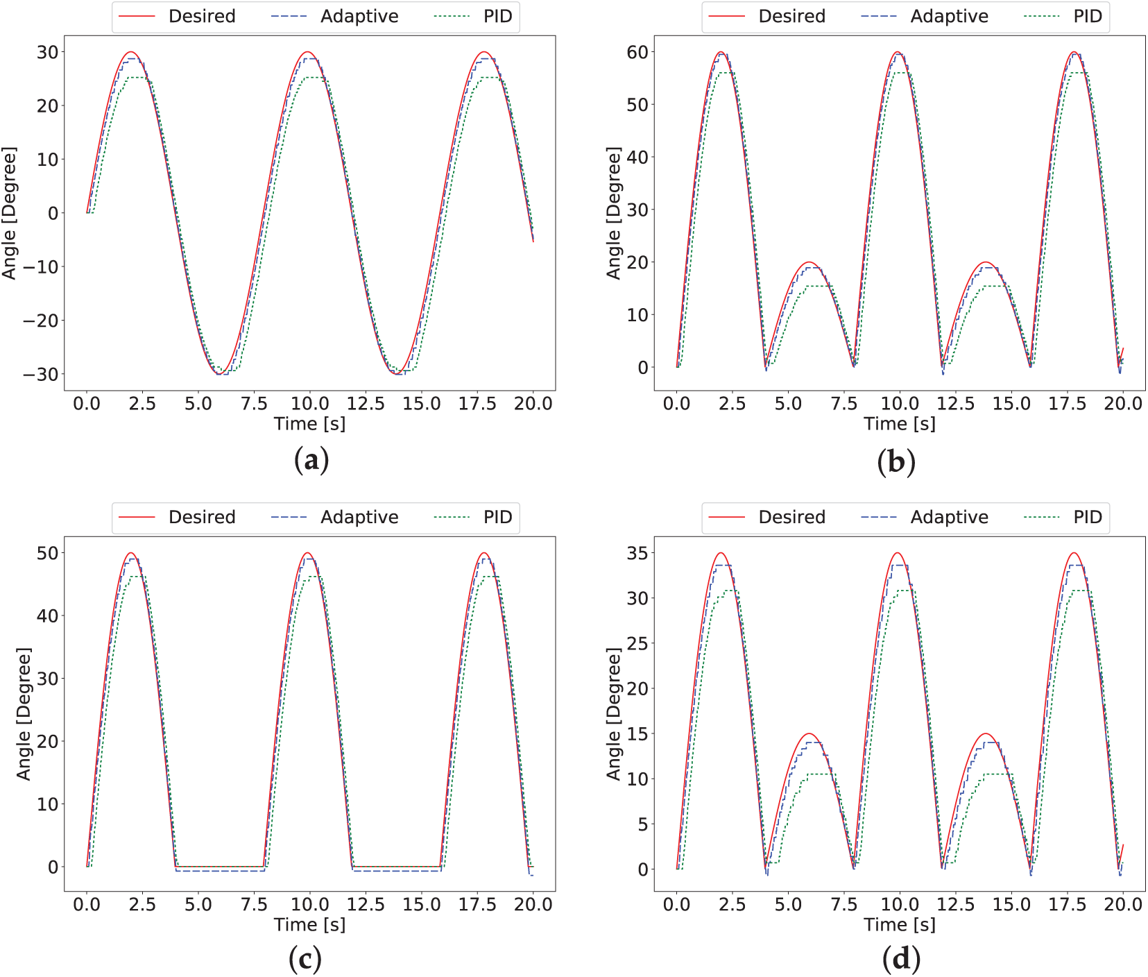
Figure 7: Comparison of tracking trajectory of our adaptive neural network controller and a conventional PID controller of each joint. (a) SR (b) SP (c) EP (d) WY

The Root Mean Square (RMS) of the tracking error had been determined as shown in Table 2. This table compares the propsed daptive neural network controller, PID controller from [38], NFAC from [22], as well as AFC from [27].

The adaptive neural network controller exhibited a smaller RMS value compared to the conventional PID controller. The adaptive neural network control scheme, which incorporated a disturbance observer, established a more instinctive interaction between the human and robot than the method mentioned in [22,27]. For instance, the performance of the Adaptive Neural Network Controller for Joint 4 (WY) was more efficient by 15.79%, 389.47%, and 268.42% than the NFAC controller by [22], the AFC controller by [27], and the Conventional PID controller, respectively. Therefore, our adaptive neural network controller method enabled efficient trajectory tracking even in the presence of human interaction forces and unknown disturbances.

Our adaptive neural network controller efficiently tracked defined desired trajectory that was adopted from our previous study in [37]. The disturbance observer effectively mitigated unknown disturbances, ensuring system stability using a high-dimensional integral Lyapunov function. The neural network estimator accurately estimated uncertain parameters of the nonlinear dynamic system. In summary, our adaptive neural network controller constrained the tracking error within a specified range, demonstrating its overall effectiveness. In conclusion, our adaptive control scheme has exhibited satisfactory performance and holds significant potential in the field of upper-limb exoskeletons.

5  Conclusion

This paper presentd a novel adaptive neural network controller designed for a four DoFs wearable assistive upper-limb exoskeleton. The controller ensured system stability using a high-dimensional integral-based Lyapunov function. The RBFNN estimated uncertain parameters, while a disturbance observer handled unknown disturbances. The adaptive neural network controller aimed to accurately track the exoskeleton’s desired trajectory for target joints.

Four human-interaction-based scenarios were conducted to assess the controller’s effectiveness. Results revealed that the adaptive neural network controller bounded tracking errors within a specific range, surpassing the conventional PID controller in terms of efficiency and performance. The proposed controller achieved a significant improvement in RMS tracking error over several benchmark methods, reducing the error by 73% compared to the conventional PID controller, by 15.8% compared to the NFAC, and by an impressive 389% compared to the AFC method.

Although our adaptive neural network controller exhibited impressive performance, recognizing its limitations is crucial for future enhancements. Future research could focus on refining control parameters to attain a higher level of precision and adaptability. Intelligent algorithms based on human interaction movements could be employed to train disturbance observer parameters. Also, future studies could explore hybridizing our control framework with reinforcement learning for adaptive parameter tuning or Gaussian processes for uncertainty quantification. Incorporating the wearer’s estimation strategy into training may further enhance the disturbance observer’s efficiency and overall performance.

Acknowledgement: The authors extend their appreciation to the King Salman Center For Disability Research for funding this work through Research Group No. KSRG-2024-468.

Funding Statement: This research was funded by the King Salman Center For Disability Research, through Research Group No. KSRG-2024-468.

Author Contributions: Conceptualization, Mohammad Soleimani Amiri, Sahbi Boubaker, Souad Kamel and Rizauddin Ramli; methodology, Mohammad Soleimani Amiri and Rizauddin Ramli; software, Mohammad Soleimani Amiri; validation, Mohammad Soleimani Amiri, Rizauddin Ramli and Sahbi Boubaker; formal analysis, Mohammad Soleimani Amiri, Rizauddin Ramli and Sahbi Boubaker; investigation, Mohammad Soleimani Amiri, Souad Kamel and Rizauddin Ramli; resources, Mohammad Soleimani Amiri; data curation, Mohammad Soleimani Amiri, Souad Kamel and Rizauddin Ramli; writing—original draft preparation, Mohammad Soleimani Amiri; writing—review and editing, Sahbi Boubaker, Rizauddin Ramli and Souad Kamel; visualization, Mohammad Soleimani Amiri; supervision, Rizauddin Ramli; project administration, Sahbi Boubaker; funding acquisition, Sahbi Boubaker. All authors reviewed the results and approved the final version of the manuscript.

Availability of Data and Materials: Due to the nature of this research, participants of this study did not agree for their data to be shared publicly, so supporting data is not available.

Ethics Approval: Not applicable

Conflicts of Interest: The authors declare no conflicts of interest to report regarding the present study.

References

1. Zipser CM, Cragg JJ, Guest JD, Fehlings MG, Jutzeler CR, Anderson AJ, et al. Cell-based and stem-cell-based treatments for spinal cord injury: evidence from clinical trials. Lancet Neurol. 2022;21(7):659–70. doi:10.1016/S1474-4422(21)00464-6. [Google Scholar] [PubMed] [CrossRef]

2. Lin PH, Dong Q, Chew SY. Injectable hydrogels in stroke and spinal cord injury treatment: a review on hydrogel materials, cell-matrix interactions and glial involvement. Mat Adv. 2021;2(8):2561–83. doi:10.1039/d0ma00732c. [Google Scholar] [CrossRef]

3. Wang J, Pei S, Guo J, Bao M, Yao Y. A vector-based motion retargeting approach for exoskeletons with shoulder girdle mechanism. Biomimetics. 2025;10(5):312–27. doi:10.3390/biomimetics10050312. [Google Scholar] [PubMed] [CrossRef]

4. Zhou J, Yang S, Xue Q. Lower limb rehabilitation exoskeleton robot: a review. Adv Mech Eng. 2021;13(4):16878140211011862. doi:10.1177/16878140211011862. [Google Scholar] [CrossRef]

5. Wang T, Chenhao BZL, Liu T, Han Y, Ferreira SWJP, Dong W, et al. A review on the rehabilitation exoskeletons for the lower limbs of the elderly and the disabled. Electronics. 2022;11(3):1–16. doi:10.3390/electronics11030388. [Google Scholar] [CrossRef]

6. Joel JPA, Raj RJS, Muthukumaran N. Review on gait rehabilitation training using human adaptive mechatronics system in biomedical engineering. In: 2022 International Conference on Computer Communication and Informatics (ICCCI); 2022 Jan 25–27; Coimbatore, India. p. 1–5. doi:10.1109/ICCCI54379.2022.9740794. [Google Scholar] [CrossRef]

7. Xia Y, Li J, Yang D, Wei W. Gait phase classification of lower limb exoskeleton based on a compound network model. Symmetry. 2023;15(1):163. doi:10.3390/sym15010163. [Google Scholar] [CrossRef]

8. Cortese M, Cempini M, De Almeida R, Paulo R, Soekadar SR, Carrozza MC, et al. A Mechatronic system for robot-mediated hand telerehabilitation. IEEE/ASME Trans Mechatr. 2015;20(4):1753–64. doi:10.1109/TMECH.2014.2353298. [Google Scholar] [CrossRef]

9. Mohammadi M, Knoche H, Thøgersen M, Bengtson SH, Kobbelgaard FV, Gull MA, et al. Tongue control of a five-DOF upper-limb exoskeleton rehabilitates drinking and eating for individuals with severe disabilities. Int J Hum Comput Stud. 2023;170(10):102962. doi:10.1016/j.ijhcs.2022.102962. [Google Scholar] [CrossRef]

10. Qin L, Wang ZXJ, Lu G, Ji H. Control method in coordinated balance with the human body for lower-limb exoskeleton rehabilitation robots. Biomimetics. 2025;10(5):324–48. doi:10.3390/biomimetics10050324. [Google Scholar] [PubMed] [CrossRef]

11. Song X, Yi B, Chen Q, Zhou Y, Cho H, Hong Y, et al. Machine learning-powered ultrahigh controllable and wearable magnetoelectric piezotronic touching device. Am Chem Soc. 2024;18(26):16648–57. doi:10.1021/acsnano.4c01102. [Google Scholar] [PubMed] [CrossRef]

12. Shi D, Zhang W, Zhang W, Ding X. A review on lower limb rehabilitation exoskeleton robots. Chin J Mech Eng. 2019;32(1):74. (In English). doi:10.1186/s10033-019-0389-8. [Google Scholar] [CrossRef]

13. Rahmani M, Rahman MH. An upper-limb exoskeleton robot control using a novel fast fuzzy sliding mode control. J Intell Fuzzy Syst. 2019;36(3):2581–92. doi:10.3233/JIFS-181558. [Google Scholar] [CrossRef]

14. Razzaghian A. A fuzzy neural network-based fractional-order Lyapunov-based robust control strategy for exoskeleton robots: application in upper-limb rehabilitation. Mathem Comput Simulat. 2022;193(22):567–83. doi:10.1016/j.matcom.2021.10.022. [Google Scholar] [CrossRef]

15. Zhao J, Zhang Y, Hou H, Yue Y, Meng K, Yang Z. Active disturbance rejection control with backstepping for decoupling control of hydraulic driven lower limb exoskeleton robot. IEEE Trans Indust Elect. 2025;72(1):714–23. doi:10.1109/TIE.2024.3413820. [Google Scholar] [CrossRef]

16. Zhang X, Wang H, Tian Y, Peyrodie L, Wang X. Model-free based neural network control with time-delay estimation for lower extremity exoskeleton. Neurocomputing. 2018;272(10):178–88. doi:10.1016/j.neucom.2017.06.055. [Google Scholar] [CrossRef]

17. Yang Y, Huang D, Dong X. Enhanced neural network control of lower limb rehabilitation exoskeleton by add-on repetitive learning. Neurocomputing. 2019;323(4):256–64. doi:10.1016/j.neucom.2018.09.085. [Google Scholar] [CrossRef]

18. AL-Dujaili AQ, Hasan AF, Humaidi AJ, Al-Jodah A. Anti-disturbance control design of Exoskeleton Knee robotic system for rehabilitative care. Heliyon. 2024;10(9):e28911. doi:10.1016/j.heliyon.2024.e28911. [Google Scholar] [PubMed] [CrossRef]

19. Jabbari Asl H, Narikiyo T, Kawanishi M. Neural network-based bounded control of robotic exoskeletons without velocity measurements. Control Eng Pract. 2018;80(12):94–104. doi:10.1016/j.conengprac.2018.08.005. [Google Scholar] [CrossRef]

20. Wu Q, Zheng L, Zhu Y, Xu Z, Zhang Q, Wu H. Development of a reconfigurable 7-DOF upper limb rehabilitation exoskeleton with gravity compensation based on DMP. IEEE Trans Med Robot Bionics. 2025;7(1):303–14. doi:10.1109/TMRB.2024.3517157. [Google Scholar] [CrossRef]

21. Alawad NA, Humaidi AJ, S Alaraji A. Sliding mode-based active disturbance rejection control of assistive exoskeleton device for rehabilitation of disabled lower limbs. An Da Acad Bras De Cienc. 2023;95(2):e20220680. doi:10.1590/0001-3765202320220680. [Google Scholar] [PubMed] [CrossRef]

22. Wu Q, Wagn X, Chen B, Wu H. Development of an RBFN-based neural-fuzzy adaptive control strategy for an upper limb rehabilitation exoskeleton. Mechatronics. 2018;53(3):85–94. doi:10.1016/j.mechatronics.2018.05.014. [Google Scholar] [CrossRef]

23. Liu Q, Liu Y, Zhu C, Guo X, Meng W, Ai Q, et al. Design and control of a reconfigurable upper limb rehabilitation exoskeleton with soft modular joints. IEEE Access. 2021;9:166815–24. doi:10.1109/ACCESS.2021.3136242. [Google Scholar] [CrossRef]

24. Zhang G, Wang J, Yang P, Guo S. A learning control scheme for upper-limb exoskeleton via adaptive sliding mode technique. Mechatronics. 2022;86(2):102832. doi:10.1016/j.mechatronics.2022.102832. [Google Scholar] [CrossRef]

25. Han S, Wang H, Tian Y, Christov N. Time-delay estimation based computed torque control with robust adaptive RBF neural network compensator for a rehabilitation exoskeleton. ISA Trans. 2020;97(2):171–81. doi:10.1016/j.isatra.2019.07.030. [Google Scholar] [PubMed] [CrossRef]

26. He D, Wang H, Tian Y, Guo Y. A fractional-order ultra-local model-based adaptive neural network sliding mode control of n-DOF upper-limb exoskeleton with input deadzone. IEEE/CAA J Autom Sin. 2024;11(3):760–81. doi:10.1109/JAS.2023.123882. [Google Scholar] [CrossRef]

27. Huang P, Li Z, Zhou M, Li X, Cheng M. Fuzzy enhanced adaptive admittance control of a wearable walking exoskeleton with step trajectory shaping. IEEE Trans Fuzzy Syst. 2022;30(6):1451–552. doi:10.1109/tfuzz.2022.3162700. [Google Scholar] [CrossRef]

28. Amiri MS, Ramli R, Aliman N. Adaptive swarm fuzzy logic controller of multi-joint lower limb assistive robot. Machines. 2022;10(6):425. doi:10.3390/machines10060425. [Google Scholar] [CrossRef]

29. Ruiz-Ruiz FJ, Ventura J, Urdiales C, Gómez-de-Gabriel JM. Compliant gripper with force estimation for physical human-robot interaction. Mech Mach Theory. 2022;178(8):105062. doi:10.1016/j.mechmachtheory.2022.105062. [Google Scholar] [CrossRef]

30. Amiri MS, Ramli R. Utilisation of initialised observation scheme for multi-joint robotic arm in Lyapunov-based adaptive control strategy. Mathematics. 2022;10(17):3126. doi:10.3390/math10173126. [Google Scholar] [CrossRef]

31. Zhang L, Li Z, Yang C. Adaptive neural network based variable stiffness control of uncertain robotic systems using disturbance observer. IEEE Trans Indus Elect. 2017;64(3):2236–45. doi:10.1109/TIE.2016.2624260. [Google Scholar] [CrossRef]

32. Voigtlaender F. The universal approximation theorem for complex-valued neural networks. Appl Comput Harmon Anal. 2023;46(04):33–61. doi:10.1016/j.acha.2022.12.002. [Google Scholar] [CrossRef]

33. Anand A, Seel K, Gjærum V, Håkansson A, Robinson H, Saad A. Safe learning for control using control Lyapunov functions and control barrier functions: a review. Procedia Comput Sci. 2021;192(4-5):3987–97. doi:10.1016/j.procs.2021.09.173. [Google Scholar] [CrossRef]

34. Shi W. Adaptive fuzzy output-feedback control for nonaffine MIMO nonlinear systems with prescribed performance. IEEE Trans Fuzzy Syst. 2021;29(5):1107–20. doi:10.1109/TFUZZ.2020.2969110. [Google Scholar] [CrossRef]

35. Yang Y, Cui Y, Qiao J, Zhu Y. Adaptive periodic-disturbance observer based composite control for SGCMG gimbal servo system with rotor vibration. Control Eng Pract. 2023;132(2):105407. doi:10.1016/j.conengprac.2022.105407. [Google Scholar] [CrossRef]

36. Qiu Z, Duan C, Yao W, Zeng P, Jiang L. Adaptive Lyapunov function method for power system transient stability analysis. IEEE Trans Power Syst. 2023;38(4):3331–44. doi:10.1109/TPWRS.2022.3199448. [Google Scholar] [CrossRef]

37. Amiri MS, Ramli R. Fuzzy adaptive controller of a wearable assistive upper limb exoskeleton using a disturbance observer. IEEE Trans Human-Mach Syst. 2025;55(2):197–206. doi:10.1109/THMS.2025.3529759. [Google Scholar] [CrossRef]

38. Amiri MS, Ramli R, Van M. Swarm-initialized adaptive controller with beetle antenna searching of wearable lower limb exoskeleton for sit-to-stand and walking motions. ISA Trans. 2025;158(5):640–53. doi:10.1016/j.isatra.2025.01.003. [Google Scholar] [PubMed] [CrossRef]

39. Amiri MS, Ramli R. Offline tuning mechanism of joint angular controller for lower-limb exoskeleton with adaptive biogeographical-based optimization. Turk J Elect Eng Comput Sci. 2022;30(4):1654. doi:10.55730/1300-0632.3871. [Google Scholar] [CrossRef]