
 Submit a Paper
 Propose a Special lssue
 Open Access
ARTICLE

Computational Solutions of a Delay-Driven Stochastic Model for Conjunctivitis Spread
1 Center for Research and Development in Mathematics and Applications (CIDMA), Department of Mathematics, University of Aveiro, Aveiro, 3810-193, Portugal
2 Department of Physical Sciences, The University of Chenab, Gujrat, 50700, Pakistan
3 Department of Computer Science and Mathematics, Lebanese American University, Beirut, 1102 2801, Lebanon
4 Department of Mathematical Sciences, College of Science, Princess Nourah bint Abdulrahman University, P.O. Box 84428, Riyadh, 11671, Saudi Arabia
5 Department of Mathematics and Statistics, College of Science, King Faisal University, Al Ahsa, 31982, Saudi Arabia
* Corresponding Authors: Ali Raza. Email: ; Emad Fadhal. Email:
(This article belongs to the Special Issue: Recent Developments on Computational Biology-II)
Computer Modeling in Engineering & Sciences 2025, 144(3), 3433-3461. https://doi.org/10.32604/cmes.2025.069655
Received 27 June 2025; Accepted 12 August 2025; Issue published 30 September 2025
 View Full Text
 Download PDF
Abstract
This study investigates the transmission dynamics of conjunctivitis using stochastic delay differential equations (SDDEs). A delayed stochastic model is formulated by dividing the population into five distinct compartments: susceptible, exposed, infected, environmental irritants, and recovered individuals. The model undergoes thorough analytical examination, addressing key dynamical properties including positivity, boundedness, existence, and uniqueness of solutions. Local and global stability around the equilibrium points is studied with respect to the basic reproduction number. The existence of a unique global positive solution for the stochastic delayed model is established. In addition, a stochastic nonstandard finite difference scheme is developed, which is shown to be dynamically consistent and convergent toward the equilibrium states. The scheme preserves the essential qualitative features of the model and demonstrates improved performance when compared to existing numerical methods. Finally, the impact of time delays and stochastic fluctuations on the susceptible and infected populations is analyzed.Keywords
Conjunctivitis, often called pink eye, is a highly contagious disease. Infection of the conjunctiva is generally a result of viruses, bacteria, and allergens. Some viruses can cause a precise conjunctivitis known as acute hemorrhagic conjunctivitis (AHC). Bacterial conjunctivitis causes the speedy onset of conjunctiva irritation, puffiness of the eyelid, and a muggy release. Usually, signs advance mainly in a single eye and then may extend to the next eye within 2 to 5 days. Three main viruses have been studied and built as the agents responsible for acute hemorrhagic conjunctivitis (AHC): coxsackievirus A24 variation (CA24v), enterovirus 70, and adenovirus 11. Acute hemorrhagic conjunctivitis (AHC) can only occur in a human population and is transmitted through human interaction with an infected specific object, like a towel used by a diseased person. The discomfort of the eyes, sensitivity to light, sore eyes, tears, and pus discharge are some symptoms. Antibiotic eye drops, sanitized passivity, quarantine, and permitting the infection to progress in 2–3 weeks are operative ways to break the extent of conjunctivitis infection [1]. Recently, a significant outbreak occurred in different cities in Pakistan. It began in Karachi and spread to major cities. Almost one hundred thousand cases were reported in Punjab. This massive outbreak of pink eye is a recent development in Pakistan’s history [2].
In 2024, Faisal et al. [3] examined the dynamics of conjunctivitis adenovirus using a unique tool such as bifurcation. At the end, to support the dynamical results, they simulated their numerical result very comprehensively. Gabriela et al. [4] conducted a study in 2024 using a basic Susceptible-Infectious-Susceptible (SIS) model with introducing uncertainty through transmission parameters. They attained conditions of extinction and existence using threshold constraints. They considered real-world problems and proposed suitable uncertain parameters. In 2024, Essak [5] considered three types of uncertainty in their study Lévy noise, Gaussian white noise, and telegraph noise to investigate their influence on the dynamics of disease. Albani et al. [6] used the fact that model parameters evolve with time and showed the randomness of sudden change. They proposed the jump-diffusion stochastic process. They presented their dynamical analysis and compared it with the variation and jumps. They used real data for their simulation and claimed their finding are accurate. In 2024, Ali et al. [7] considered a stochastic model for influenza dynamics and also used accurate parameter values for their comprehensive understanding of influenza dynamics. They used actual data for their simulation that supports their dynamic results. In 2014, Unyong et al. [8] suggested and investigated a mathematical system for the dynamical stability of conjunctivitis with nonlinear incidence terms considered. Finally, numerical results support the analytic results. In 2012, Sangsawang et al. [9] investigated the system for the spread of Hemorrhagic Conjunctivitis. Numerical simulations of the system demonstrate that the disease-free equilibrium and endemic are stable and unique. In 2006, Chowell et al. [10] modeled the diffusion dynamics of AHC in an eruption of pink eye in the host population in Mexico. Therefore, the effects of sustenance present a public health strategy and the efficient message of the eruption, and community health evidence press statements that initiate beings on evading infection and encourage them to pursue a clinical diagnosis. They studied epidemic models with well-known computational methods based on stochastic differential equations with artificial decay terms in [11–13]. They studied well-known stochastic models such as the stochastic within-host Chikungunya (CHIKV) virus model with saturated incidence rate, Extinction, and the stationary distribution of the stochastic hepatitis B virus model, and a Zika virus as a mosquito-borne transmitted disease with environmental fluctuations as presented in [14–16]. The approach aligns with recent works such as [17], where stochastic noise is interpreted as environmental randomness impacting disease spread. Foundational contributions such as those in [18] provide detailed bifurcation analysis of delay epidemic models, highlighting the critical role of time-lag in disease dynamics. Similarly, reviews in [19,20] summarize analytical techniques for deterministic and stochastic delay systems, particularly in biological contexts. Our model structure and analytical proofs draw on these theoretical foundations, especially in establishing positivity, stability, and global existence. The authors studied the Split-Step θ-Method for Stochastic Pantograph Differential Equations, focusing on convergence and mean-square stability analysis, in [21].
Model formation and its numerical simulations are the classical origins of studying the transmission dynamics of infectious diseases because they allow us to understand the complex transmission dynamics of any contagious disease. The trajectories of the deterministic model are idealistic, but the stochastic model is closer to reality. This outcome matters for policymakers and concerned individuals. So, this study took the deterministic model and reformulated it into a stochastic delayed conjunctivitis model, then studied its stochastic behavior to understand the dynamics of the spread of disease, and an exponential delay was introduced to understand the effect of delay on the spread of disease to get more optimal results to control the disease. This work makes several novel contributions to the modeling and control of conjunctivitis epidemics:
• Model Innovation: The stochastic delayed compartment model for conjunctivitis is configured in a new manner such that it incorporates artificial delay effects to reflect realistic intervention strategies such as quarantine, delayed exposure, or behavioral response to symptoms.
• Theoretical Advancement: The model’s dynamical properties, including positivity, boundedness, existence, and uniqueness, were studied rigorously. Also, the authors studied local and global stability conditions under biologically meaningful assumptions.
• Numerical Methodology: A completely new and original stochastic nonstandard finite difference (NSFD) method has been developed and analyzed. This method retains important dynamical properties, ensures numerical positivity and convergence, and beats standard methods under larger time steps.
• Biological Insight: Artificial delays significantly reduce the number of infected individuals and increase the susceptible population, with use as a control strategy. These findings are compatible with recent public health approaches and have practical relevance to the model.
• Literature Integration: This paper contributes to filling the gap in existing literature by making an extended union of stochastic dynamics, artificial delays, and conjunctivitis modeling under one united framework, which is justified by the most recent epidemiological events and data.
• Public Health Interpretation of Artificial Delay: The exponential delay term
The mathematical framework of this study is deeply rooted in functional analysis. This study employs key results from functional analysis, including fixed point theory, operator norms, and stability criteria in infinite-dimensional spaces, to establish existence, uniqueness, and positivity of solutions. These foundational tools ensure the rigorous formulation and analysis of the stochastic delay differential equations (SDDEs) that govern the proposed model.
The following subdivisions comprise five sections: Section 1 briefly introduces the research disease and literature review. Section 2 presents the derivation of the delayed mathematical model and its dynamical properties, equilibrium points, and local-global behavior of the delayed system. Section 3 describes the stochastic delayed model and the theorem-related unique global positive solution. Section 4 introduces the selective numerical method, and presents the derived stochastic NSFD-related theorems. Lastly, Section 5 discusses numerical simulations among selective techniques and their convergence behavior around the conjunctivitis present state with different step sizes. In addition, the discussion and conclusion are presented in different sections.
2 Derivation of the Delayed Conjunctivitis Mathematical Model
This model is present in [1] in the deterministic form. This study investigates artificial delay effects and stochastic behaviors to understand the realistic transmission dynamics. Delay-based interventions are used to control the spread of disease. Because of the exponential growth of the disease population, the exponential delay is employed to prevent disease transmission similarly. In [1], the human host population N(t) is divided into five compartments
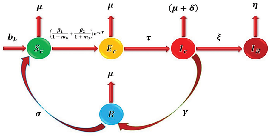
Figure 1: Flow dynamics of the Conjunctivitis disease in a population
The delayed conjunctivitis mathematical model is derived under the following assumptions.
• Direct and indirect transmission paths are taken.
• Individuals who recover again become susceptible to the disease.
• Individuals who lost their vision are considered.
• The host population is equally mixed.
• The natural death rate and birth rate are the same.
• The natural death rate and natural expiry rate of bacteria/viruses are approximately equal.
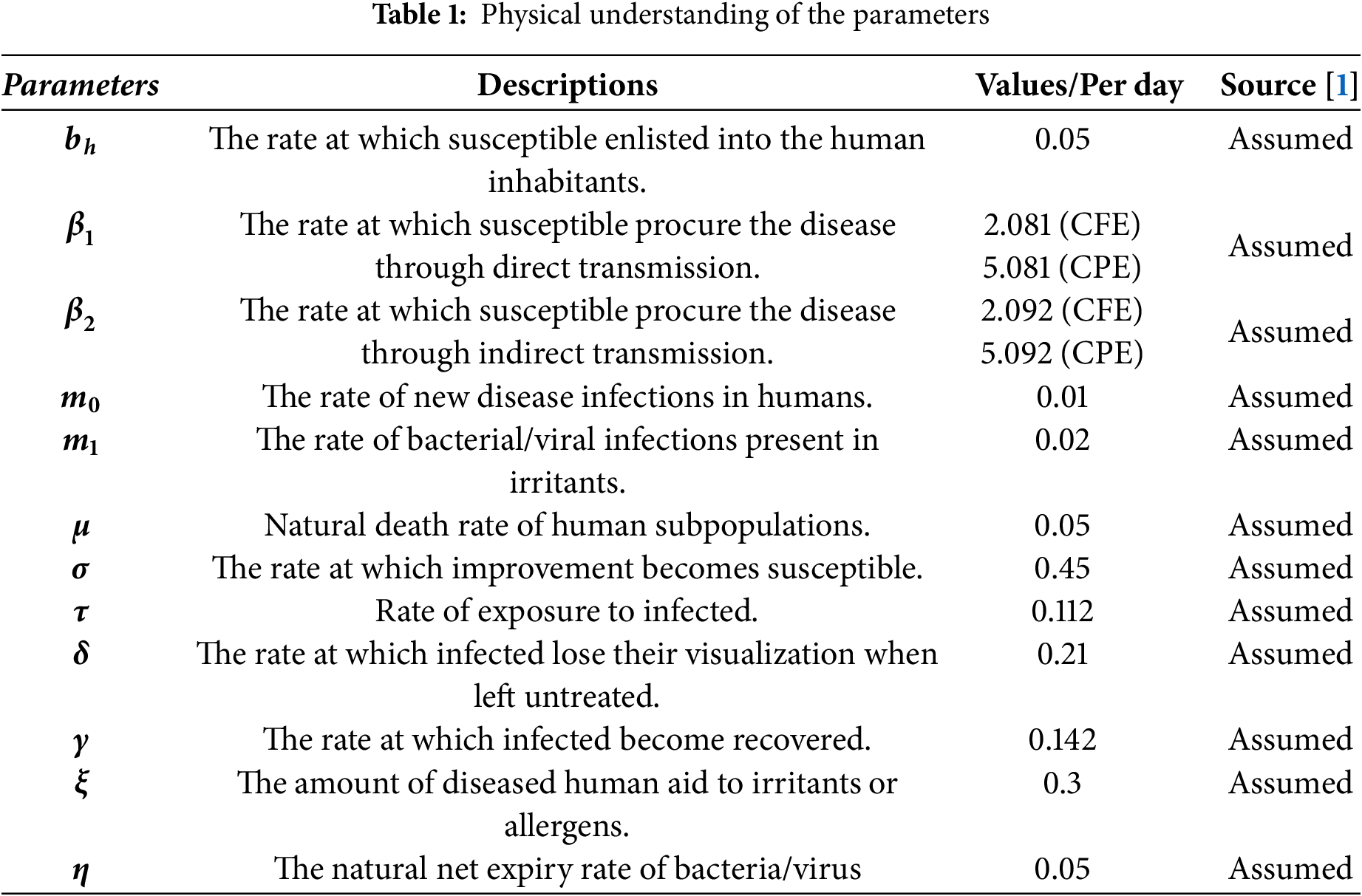
Although most parameter values are directly adopted from [1], several minor modifications were made to improve computational tractability and biological interpretability. Specifically, this study assumes that the birth and natural death rates are equal (0.05/day), a common simplification in epidemic models to maintain a stable total population in the absence of disease-related deaths. This assumption allows a clearer focus on the disease-induced dynamics without the confounding effects of demographic growth or decline.
The model of the conjunctivitis delay differential equations is as follows:
Given that
Theorem 1: (Positivity) For any given initial condition
Proof: If
Similarly, the following relationships from system (2)–(5) can be described:
Eqs. (6)–(10) are non-negative. Hence, the system (1)–(5) is positive
Theorem 2: (Boundedness)
Proof: After adding the system (1)–(5), the total population of the system is as follows:
The general solution
Now, any given initial trajectory
Theorem 3: (Existence and Uniqueness) The unique solution of system (1)–(5) exists piece-wise if it satisfies linear growth and Lipschitz conditions and
Proof: Define the norm
Considering system (1)–(5) yields:
The uniqueness of Eq. (12) can be proved by satisfying Eq. (13) as follows:
The condition
Similar,
The condition
The condition
The condition
The condition
Now, Lipschitz’s condition is verified for the existence as follows:
Eqs. (15)–(19) indicate that systems (1)–(5) have unique solutions and Eqs. (20)–(24) have a sure existence. □
To obtain the condition where conjunctivitis dies out from the system (1)–(5) or becomes endemic.
To determine the system’s reproductive number [22] of (1)–(5) using the following generation matrix method.
Theorem 4: The reproductive number of the system (1)–(5) is given by
Proof: By the abovementioned method, three concerned compartments are considered,
Now,
here,
and
where
Hence, by the largest eigenvalue of
Now, the asymptotic behaviour of convergence for the system (1)–(5) is investigated locally and globally around defined equilibrium states with the constraints of the reproductive number.
Theorem 5: (Local stability at
Proof: To prove this result, the Jacobian matrix of the right-side system (1)–(5) at
For eigenvalue,
By expanding (28),
where
Theorem 6: (Local stability at
Proof: To prove this result, the Jacobian matrix of system (1)–(5) at
Routh-Hurwitz criteria for the 5th-order polynomial exhibit that all the eigenvalues of (30) through MATLAB have negative real parts. Hence, the system (1)–(5) at the conjunctivitis-present equilibrium point
Theorem 7: (Global stability at
Proof: Define Lyapunov function V:
if
Hence, system (1)–(5) asymptotically converges around the Conjunctivitis Free State globally if
Theorem 8: (Global stability at
Proof: Describe Lyapunov function V:
Using the right side of the system (1)–(5):
Hence, by LaSalle’s invariance principle, at
3 Stochastic Delayed Conjunctivitis Model
Now, the stochastic behavior of the system (1)–(5) is derived by the non-parametric perturbation method for more realistic optimal outcomes. So, by non-parametric perturbation technique [23], the system (1)–(5) becomes:
Given that
Unique Global Positivity
To prove the system (31) of SDDEs,
The coefficient of the system (31) is locally Lipschitz (Theorem 5.2.8, [24]), but it has a linear growth property. Thus, it can explode to infinity at a finite time. To prove a unique global solution, it is enough to prove
Theorem 9: For system (31) any given initial value
Proof: Since the coefficient of the system (31) is locally Lipschitz, a unique maximal local solution exists for any given initial condition.
Suppose
Prove this result by contradiction, then there exists
This, there is an integer
For any K such that
The following can be calculated using Ito’s formula:
If
After integrating from 0 to
Using the fact E
Set
Hence,
The indicator function is represented by
It tends to be a contradiction because
here,
This section presents the numerical competitive analysis for the stochastic delayed conjunctivitis model (31) among three standard and one nonstandard method. In which for all
4.1 Transition Probabilities of the Model
If
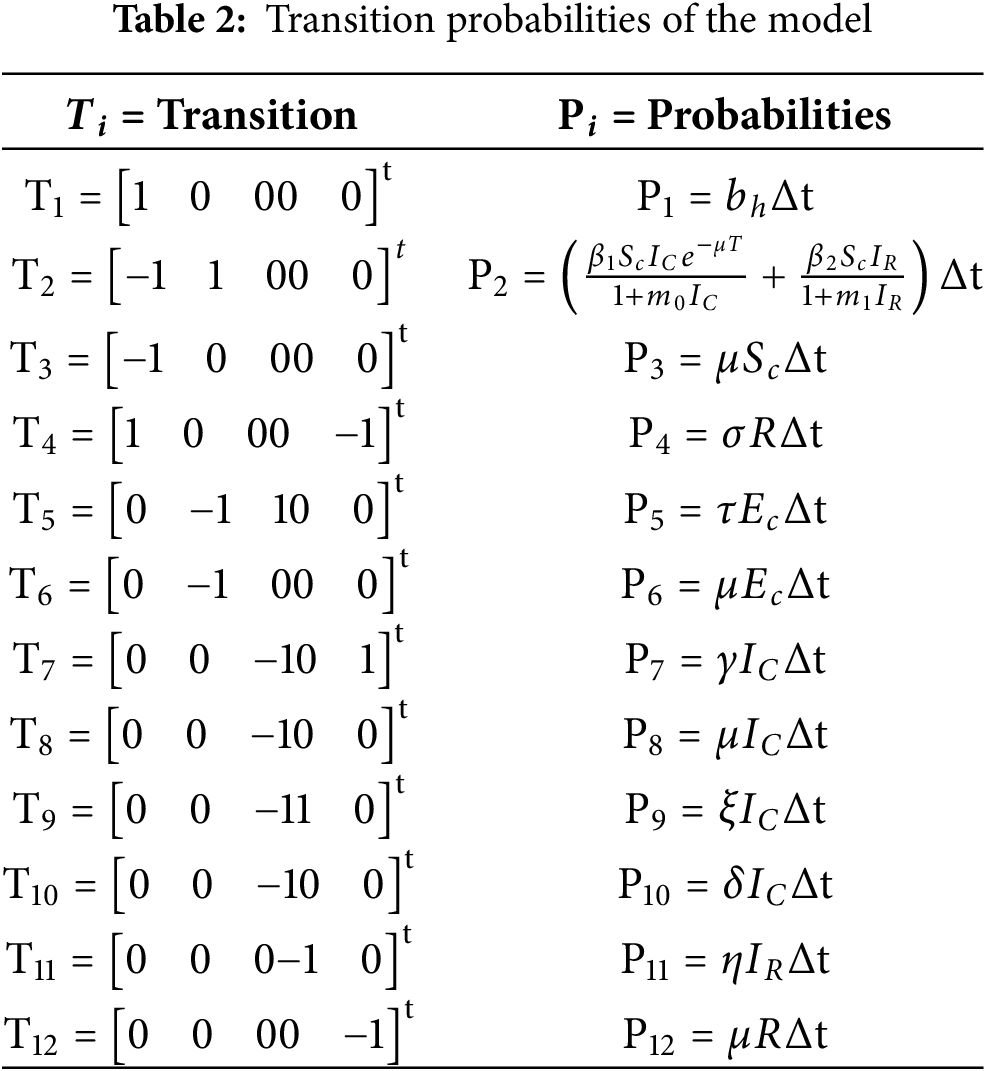
The expectation and variance of the system (31) can be described as follows:
If Drift
Eq. (37) is the stochastic differential equation with initial condition
In this technique, the weak order of convergence with weak order one under sufficient smoothness property [25] is higher than the firm order of convergence with substantial order 0.5 under Lipschitz and bounded growth properties on H and K of equation [26,27].
With initial condition
The stochastic Euler method can be formulated from the system (31) with given initial conditions
where,
4.4 Stochastic Runge-Kutta Method
The stochastic Runge-Kutta method of order four can be derived from the system (31) with given initial condition
Stage 1
Stage 2
Stage 3
Stage 4
Final stage
where,
4.5 Stochastic Nonstandard Finite Difference Method
The proposed stochastic NSFD method [28,29] of the non-parametric perturbation stochastic system (31) can be expressed in the following manner, with given initial condition
Similarly,
where,
4.6 Essential Properties for the Stochastic NSFD
It is important to check the essential properties of the proposed discrete system derived from the continuous stochastic delayed conjunctivitis system (31).
Theorem 10: For any given initial value (
Proof: The proof is straightforward because the constraint of biological problems is non-negative. □
Theorem 11: The region
Proof: Prove this result by mathematical induction on ‘n’. Case I is obvious.
Now for case-II
If the result is true for any
The system (41)–(45) can be decomposed as follows:
These equations are added by supposing non-perturbation is zero.
By Eq. (i) and suppose
By mathematical induction, the result is valid for the proposed NSFD method and hence is bounded for all
4.7 Consistency Analysis of Stochastic Nonstandard Finite Difference (NSFD)
Theorem 12: The equilibria for the stochastic proposed nonstandard system (41)–(45) are the same for any
Proof: By solving the system (41)–(45), and
Conjunctivitis free equilibrium (CFE) =
Conjunctivitis present equilibrium (CPE) =
Theorem 13: The deterministic form of the stochastic nonstandard computational system (41)–(45) is stable if the eigenvalue lies in the unit circle
Proof: The system (41)–(45), and
The Jacobian of the above equations:
where
At Conjunctivitis free equilibrium (CFE) =
All remaining eigenvalues lie within the unit circle as depicted in Fig. 2 by representing Eq. (47) using the parameter values provided in Table 1. Since the largest eigenvalue is shown to be less than one, it follows that the rest are also less than one, which confirms the system’s stability. □
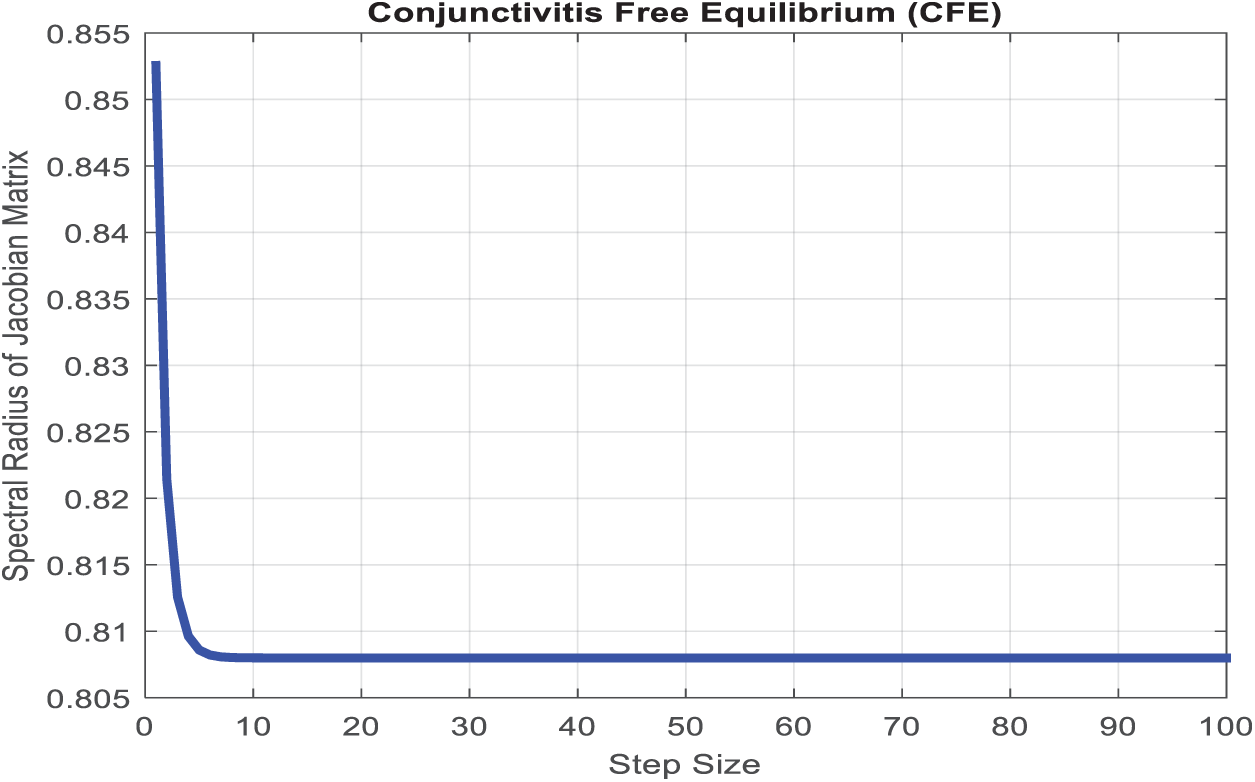
Figure 2: The spectral radius of the Jacobian matrix of the proposed nonstandard computational method at the conjunctivitis-free equilibrium (CFE) is less than one for a discrete time step size [0, 100]
Finally, the delayed nonstandard finite difference system driven by the system (41)–(45) is unconditionally asymptotically convergent to its equilibrium states for any step size.
This section presents the comparative numerical analysis of the considered standard schemes with a proposed nonstandard finite difference scheme and deterministic simulations by MATLAB. For a conjunctivitis-free state,
In the present study, the necessary dynamical properties like positivity, boundedness, uniqueness, and the existence of a conjunctivitis delayed model are studied. For small step size, Fig. 3a,c,e shows infected individuals converge to the actual endemic state, and after an increase in step size, Fig. 3b,d,f, all considered standard schemes, is inconsistent and refuses to comply with fundamental properties. In addition, the deterministic solution is the expected solution of the stochastic proposed nonstandard finite difference, which preserves all dynamic properties and a consistent scheme at any time step size. As the delay in the model increases, susceptibility exponentially rises and leads to the disease dying out from the system. Fig. 4a indicates that as the artificial delay in the model increases, the number of infected individuals decreases exponentially and, after some delay, converges to zero, and the disease dies out of the system. In contrast, Fig. 4b, in the same manner, presents an increase in the number of susceptible individuals and vice versa. Fig. 5 reveals that if
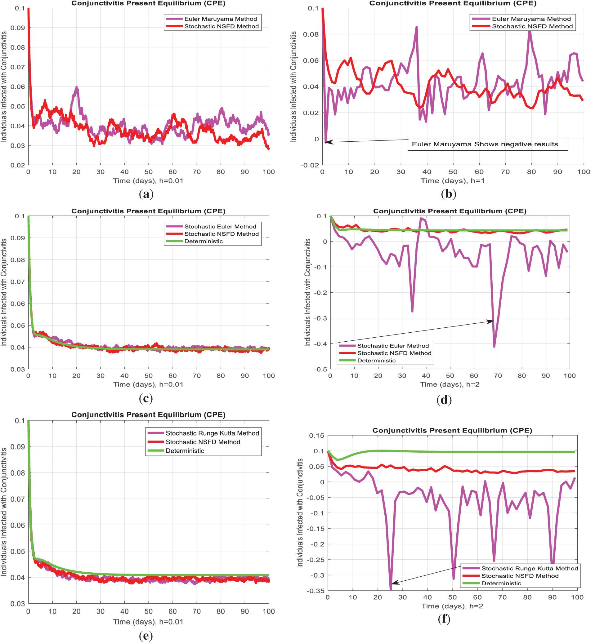
Figure 3: (a) Euler Maruyama scheme for infected individuals converges to the true endemic state for small step size h = 0.01. (b) Euler Maruyama scheme disobeys positivity for large step size
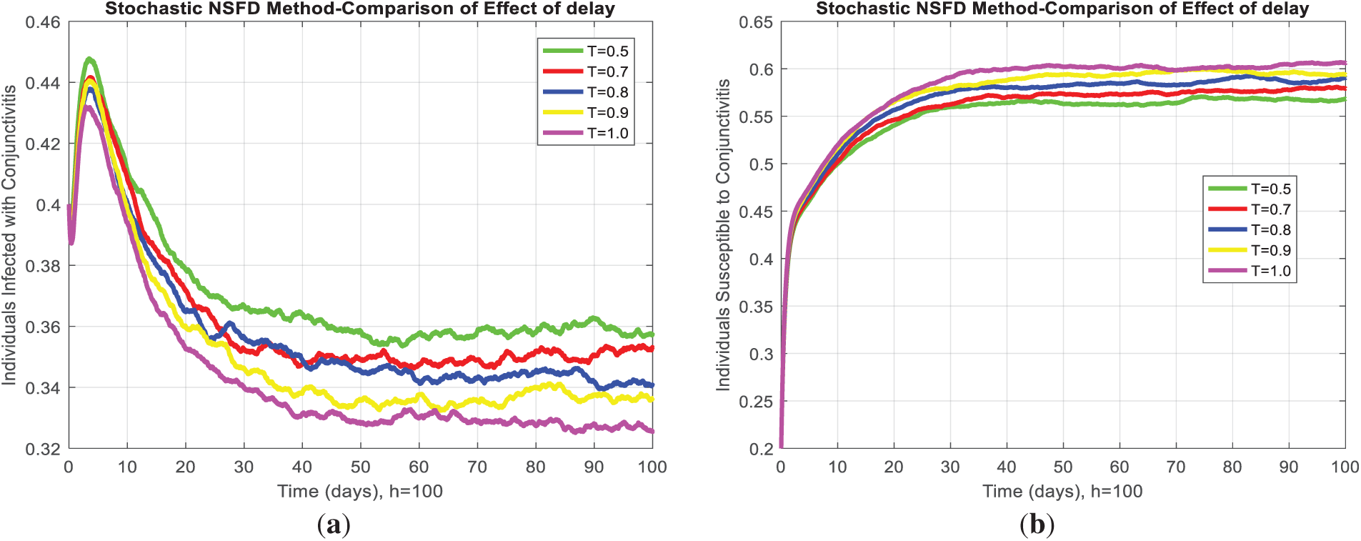
Figure 4: (a) Infected individuals decrease by increasing the delay for any step size. (b) For any step size, susceptible individuals increase whenever the delay increases
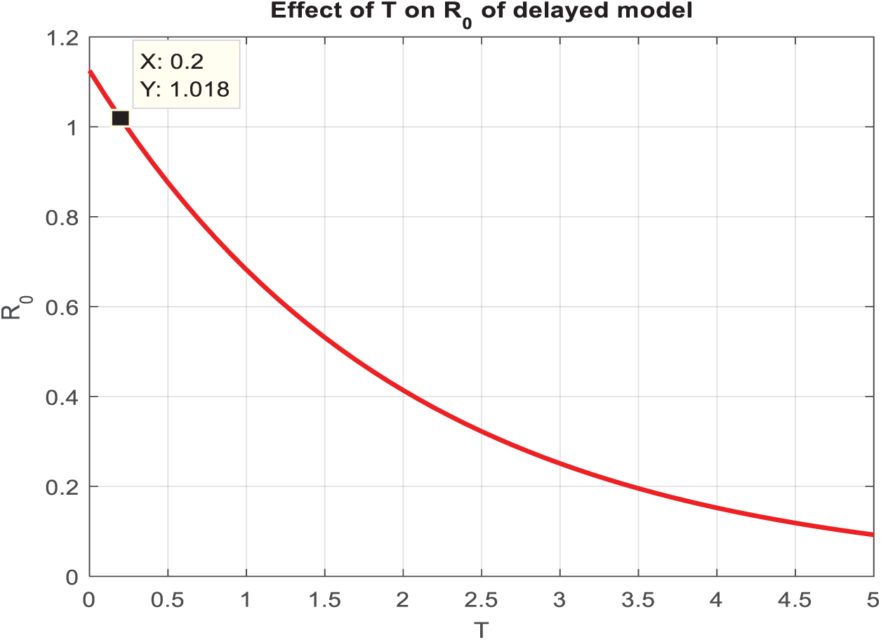
Figure 5: Almost after a three-day delay, the system changes its behavior and becomes a Conjunctivitis Free Equilibrium (CFE)
This study develops and analyzes a stochastic delay differential equation model to investigate the transmission dynamics of conjunctivitis. The model incorporates both direct and indirect transmission pathways and includes an artificial exponential delay to assess the impact of intervention strategies on disease progression. This research establishes key mathematical properties of the model, including positivity, boundedness, and the existence and uniqueness of global solutions. Stability analysis is performed around both disease-free and endemic equilibrium states under the constraint of the basic reproduction number. A novel stochastic nonstandard finite difference (NSFD) scheme is proposed, which demonstrates strong consistency with theoretical results and preserves the system’s dynamic properties across a range of time step sizes. Extensive numerical simulations indicate that artificial delay effectively reduces the number of infected individuals and promotes disease eradication, highlighting its potential as a viable public health intervention strategy. Comparison to standard numerical schemes reveals that the proposed NSFD method offers improved stability, positivity, and convergence. This study contributes a mathematically rigorous and computationally reliable framework for understanding and controlling conjunctivitis outbreaks using stochastic modeling with delay effects. The findings support the inclusion of artificial delays in epidemic models to reflect real-world disease mitigation efforts. In the future, this work could be improved by using quantum computing methods to make epidemic simulations faster and more efficient. This could allow real-time analysis and better optimization of complex disease models, especially when working with large amounts of data or uncertain situations.
Acknowledgement: All authors contributed equally. All authors read and approved the present study. This work was supported by Princess Nourah bint Abdulrahman University Researchers Supporting Project number (PNURSP2025R899), Princess Nourah bint Abdulrahman University, Riyadh, Saudi Arabia. Also, this work was supported by the Deanship of Scientific Research, Vice Presidency for Graduate Studies and Scientific Research, King Faisal University, Saudi Arabia (KFU252831).
Funding Statement: This work was supported by Princess Nourah bint Abdulrahman University Researchers Supporting Project number (PNURSP2025R899), Princess Nourah bint Abdulrahman University, Riyadh, Saudi Arabia. Also, this work was supported by the Deanship of Scientific Research, Vice Presidency for Graduate Studies and Scientific Research, King Faisal University, Saudi Arabia (KFU252831).
Author Contributions: The authors confirm contribution to the paper as follows: Ali Raza: Conceptualization, mathematical modeling, stochastic formulation, delay differential analysis, interpretation of results, supervision, writing—original draft, writing—review & editing. Asad Ullah: Data collection, computational implementation, visualization, literature review, writing—original draft. Eugénio M. Rocha: Conceptualization, model refinement, methodology, supervision, project administration, visualization, validation, writing—review & editing. Dumitru Baleanu: Model refinement, stochastic analysis, theoretical validation, critical revision, project administration. Hala H. Taha: Literature review, data analysis, interpretation of epidemiological aspects, funding acquisition, manuscript drafting, writing—review. Emad Fadhal: Validation, funding acquisition, result interpretation, manuscript writing & editing. All authors reviewed the results and approved the final version of the manuscript.
Availability of Data and Materials: The datasets analyzed during the current study are available from the corresponding authors upon reasonable request.
Ethics Approval: Not applicable.
Conflicts of Interest: The authors declare no conflicts of interest to report regarding the present study.
References
1. Ogunmiloro OM. Stability analysis and optimal control strategies of direct and indirect transmission dynamics of conjunctivitis. Math Methods App Sciences. 2020;43(18):10619–36. doi:10.1002/mma.6756. [Google Scholar] [CrossRef]
2. Pink eye outbreak in Pakistan [Internet]. [cited 2025 Aug 12]. Available from: https://en.wikipedia.org/wiki/Pink_eye_outbreak_in_Pakistan. [Google Scholar]
3. Javed F, Ahmad A, Ali AH, Hincal E, Amjad A. Investigation of conjunctivitis adenovirus spread in human eyes by using bifurcation tool and numerical treatment approach. Phys Scr. 2024;99(8):085253. doi:10.1088/1402-4896/ad62a5. [Google Scholar] [CrossRef]
4. de Jesús Cabral-García G, Villa-Morales J. Certain aspects of the SIS stochastic epidemic model. Appl Math Model. 2024;128:272–86. doi:10.1016/j.apm.2024.01.027. [Google Scholar] [CrossRef]
5. Essak AA. Stochastic differential equations in epidemiology [dissertation]. Leicester, UK: University of Leicester; 2024. [Google Scholar]
6. Albani VVL, Zubelli JP. Stochastic transmission in epidemiological models. J Math Biol. 2024;88(3):25. doi:10.1007/s00285-023-02042-z. [Google Scholar] [PubMed] [CrossRef]
7. Ali M, EL Guma F, Qazza A, Saadeh R, Alsubaie NE, Althubyani M, et al. Stochastic modeling of influenza transmission: insights into disease dynamics and epidemic management. Partial Differ Equ Appl Math. 2024;11(5):100886. doi:10.1016/j.padiff.2024.100886. [Google Scholar] [CrossRef]
8. Unyong B, Naowarat S. Stability analysis of conjunctivitis model with nonlinear incidence term. Aust J Basic Appl Sci. 2014;8(24):52–8. [Google Scholar]
9. Sangsawang S, Tanutpanit T, Mumtong W, Pongsumpun P. Local stability analysis of mathematical model for hemorrhagic conjunctivitis disease. Curr Appl Sci Technol. 2014;12(2):189–97. [Google Scholar]
10. Chowell G, Shim E, Brauer F, Diaz-Dueñas P, Hyman JM, Castillo-Chavez C. Modelling the transmission dynamics of acute haemorrhagic conjunctivitis: application to the 2003 outbreak in Mexico. Stat Med. 2006;25(11):1840–57. doi:10.1002/sim.2352. [Google Scholar] [PubMed] [CrossRef]
11. Capasso V, Serio G. A generalization of the Kermack-McKendrick deterministic epidemic model. Math Biosci. 1978;42(1–2):43–61. doi:10.1016/0025-5564(78)90006-8. [Google Scholar] [CrossRef]
12. Shafique U, Al-Shamiri MM, Raza A, Fadhal E, Rafiq M, Ahmed N. Numerical analysis of bacterial meningitis stochastic delayed epidemic model through computational methods. Comput Model Eng Sci. 2024;141(1):311–29. doi:10.32604/cmes.2024.052383. [Google Scholar] [CrossRef]
13. Raza A, Abdella K. Analysis of the dynamics of anthrax epidemic model with delay. Discov Appl Sci. 2024;6(3):128. doi:10.1007/s42452-024-05763-y. [Google Scholar] [CrossRef]
14. Shahid N, Raza A, Iqbal S, Ahmed N, Fadhal E, Ceesay B. Stochastic delayed analysis of coronavirus model through efficient computational method. Sci Rep. 2024;14(1):21170. doi:10.1038/s41598-024-70089-z. [Google Scholar] [PubMed] [CrossRef]
15. Gokila C, Sambath M. The threshold for a stochastic within-host CHIKV virus model with saturated incidence rate. Int J Biomath. 2021;14(6):2150042. doi:10.1142/s179352452150042x. [Google Scholar] [CrossRef]
16. Gokila C, Sambath M. Extinction and stationary distribution of stochastic hepatitis B virus model. Math Methods App Sciences. 2025;48(3):2913–33. doi:10.1002/mma.10467. [Google Scholar] [CrossRef]
17. Gokila C, Sambath M. Modeling and simulations of a Zika virus as a mosquito-borne transmitted disease with environmental fluctuations. Int J Nonlinear Sci Numer Simul. 2023;24(1):137–60. doi:10.1515/ijnsns-2020-0145. [Google Scholar] [CrossRef]
18. Li Y, Wei Z. Dynamics and optimal control of a stochastic coronavirus (COVID-19) epidemic model with diffusion. Nonlinear Dyn. 2022;109(1):91–120. doi:10.1007/s11071-021-06998-9. [Google Scholar] [PubMed] [CrossRef]
19. Ruan S, Wei J. On the zeros of transcendental functions with applications to stability of delay differential equations with two delays. Dyn Contin Discrete Impuls Syst Ser A Math Anal. 2003;10(6):863–74. [Google Scholar]
20. Greenhalgh D. Hopf bifurcation in epidemic models with a latent period and nonpermanent immunity. Math Comput Model. 1997;25(2):85–107. doi:10.1016/S0895-7177(97)00009-5. [Google Scholar] [CrossRef]
21. Rihan FA, Udhayakumar K. Split-step θ-method for stochastic pantograph differential equations: convergence and mean-square stability analysis. Appl Numer Math. 2025;217(3):1–17. doi:10.1016/j.apnum.2025.05.010. [Google Scholar] [CrossRef]
22. Diekmann O, Heesterbeek JP, Roberts MG. The construction of next-generation matrices for compartmental epidemic models. J R Soc Interface. 2010;7(47):873–85. doi:10.1098/rsif.2009.0386. [Google Scholar] [PubMed] [CrossRef]
23. Allen EJ, Allen LJS, Arciniega A, Greenwood PE. Construction of equivalent stochastic differential equation models. Stoch Anal Appl. 2008;26(2):274–97. doi:10.1080/07362990701857129. [Google Scholar] [CrossRef]
24. Mao X. Stochastic differential equations and applications. Amsterdam, The Netherlands: Elsevier; 2007. 448 p. [Google Scholar]
25. Gikhman II, Skorokhod AV. Stochastic differential equations. Berlin/Heidelberg, Germany: Springer; 2007. p. 113–219. [Google Scholar]
26. Mil’shtein GN. A method of second-order accuracy integration of stochastic differential equations. Theory Probab Appl. 1979;23(2):396–401. doi:10.1137/1123045. [Google Scholar] [CrossRef]
27. Talay D. Efficient numerical schemes for the approximation of expectations of functionals of the solution of a S.D.E., and applications. In: Korezlioglu H, Mazziotto G, Szpirglas J, editors. Filtering and control of random processes. Berlin/Heidelberg, Germany: Springer; 2005. p. 294–313. doi: 10.1007/bfb0006577. [Google Scholar] [CrossRef]
28. Mickens RE. Dynamic consistency: a fundamental principle for constructing nonstandard finite difference schemes for differential equations. J Differ Equ Appl. 2005;11(7):645–53. doi:10.1080/10236190412331334527. [Google Scholar] [CrossRef]
29. Mickens RE. Nonstandard finite difference schemes: methodology and applications. Singapore: World Scientific; 2020. 332 p. [Google Scholar]
30. Arenas AJ, González-Parra G, Chen-Charpentier BM. A nonstandard numerical scheme of predictor-corrector type for epidemic models. Comput Math Appl. 2010;59(12):3740–9. doi:10.1016/j.camwa.2010.04.006. [Google Scholar] [CrossRef]
Cite This Article
 Copyright © 2025 The Author(s). Published by Tech Science Press.
This work is licensed under a Creative Commons Attribution 4.0 International License , which permits unrestricted use, distribution, and reproduction in any medium, provided the original work is properly cited.
 Downloads
 Citation Tools