
 Submit a Paper
 Propose a Special lssue
 Open Access
ARTICLE

Offshore Wind Turbines Anomalies Detection Based on a New Normalized Power Index
1 Faculty of Informatics, Complutense University of Madrid, Madrid, 28040, Spain
2 Faculty of Physics, Complutense University of Madrid, Madrid, 28040, Spain
3 Institute of Knowledge Technology, Complutense University of Madrid, Madrid, 28040, Spain
* Corresponding Author: Segundo Esteban. Email:
(This article belongs to the Special Issue: Intelligent Control and Machine Learning for Renewable Energy Systems and Industries)
Computer Modeling in Engineering & Sciences 2025, 144(3), 3387-3418. https://doi.org/10.32604/cmes.2025.070070
Received 07 July 2025; Accepted 20 August 2025; Issue published 30 September 2025
 View Full Text
 Download PDF
Abstract
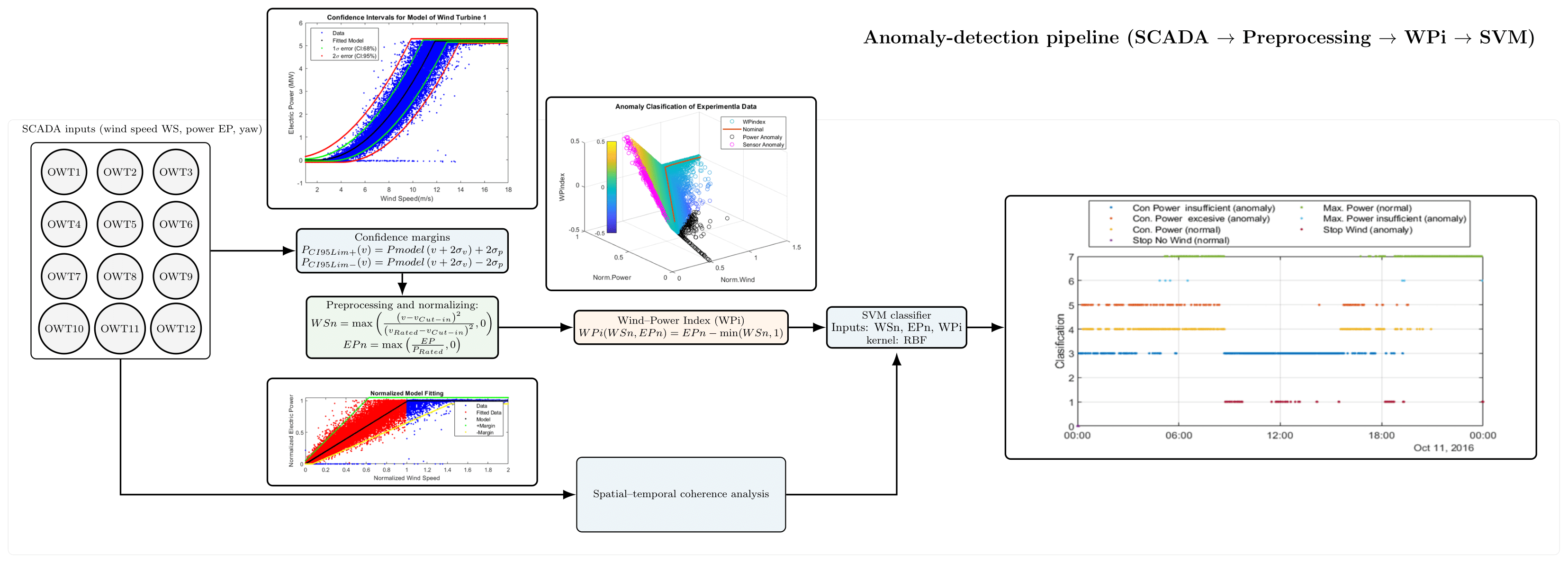
Anomaly detection in wind turbines involves emphasizing its ability to improve operational efficiency, reduce maintenance costs, extend their lifespan, and enhance reliability in the wind energy sector. This is particularly necessary in offshore wind, currently one of the most critical assets for achieving sustainable energy generation goals, due to the harsh marine environment and the difficulty of maintenance tasks. To address this problem, this work proposes a data-driven methodology for detecting power generation anomalies in offshore wind turbines, using normalized and linearized operational data. The proposed framework transforms heterogeneous wind speed and power measurements into a unified scale, enabling the development of a new wind power index (WPi) that quantifies deviations from expected performance. Additionally, spatial and temporal coherence analyses of turbines within a wind farm ensure the validity of these normalized measurements across different wind turbine models and operating conditions. Furthermore, a Support Vector Machine (SVM) refines the classification process, effectively distinguishing measurement errors from actual power generation failures. Validation of this strategy using real-world data from the Alpha Ventus wind farm demonstrates that the proposed approach not only improves predictive maintenance but also optimizes energy production, highlighting its potential for broad application in offshore wind installations.Graphic Abstract
Keywords
The rapid expansion of wind power as a key element of global strategies to extend renewable energy production has underlined the critical importance of ensuring the reliability and efficiency of wind turbines (WT). Installation and maintenance expenses currently make the largest contribution to the cost of generating this type of energy.
Offshore wind energy is becoming the backbone of energy diversification and climate change mitigation. Offshore wind farms benefit from higher and more consistent wind speeds than land-based installations, resulting in greater efficiency and more energy. In addition, they are far from communities, reducing visual and acoustic impact, and can meet significant coastal electricity demand.
But the marine environment is harsh and poses major challenges to the reliability and maintenance of these systems. Particularly, offshore wind turbines (OWT) operate in harsh and unpredictable conditions, including high winds, turbulent waves, and exposure to corrosive salt water [1]. These factors significantly increase the likelihood of mechanical and structural failures, which can lead to costly downtime, reduced energy production, and increased maintenance expenses. As OWT deployment continues to grow, the need for robust and scalable fault detection systems becomes paramount to maximize operational efficiency, longevity, and minimize economic losses [2].
However, the diversity of wind turbine designs, different manufacturers, and the varying ages of turbines in a wind farm represent a significant challenge to developing a unified approach to fault detection. Turbines of different brands often employ proprietary monitoring and metrics systems, while older turbines may lack the advanced sensors and data acquisition capabilities of newer models. This heterogeneity complicates the implementation of standardized fault detection techniques, making it difficult to compare turbine performance within the same farm or implement consistent maintenance strategies.
Therefore, it is essential to have a uniform fault detection framework that allows for the application of consistent techniques, metrics, and diagnostic tools across various turbine groups. Such a framework would not only streamline maintenance operations but also facilitate the integration of data-driven approaches, such as machine learning and predictive analytics, to improve the accuracy and speed of fault identification.
The principal motivation of this article stems from this need and is, therefore, to propose a standardized and consistent framework for fault detection in wind turbines of different brands and ages, and under different operating conditions. The objective pursued with the fault detection strategy proposed here is to establish a common basis for data management that can guarantee the reliability of the maintenance strategy and thus, to extend the useful life of wind turbines and improve their economic viability, regardless of their brand, age, or design.
However, the objective goes further by extending it to the definition of turbine health assessment metrics that examine the spatial and temporal consistency of the different wind turbines in a wind farm. These metrics capture correlations between wind turbines and trends over time, further improving the robustness of detection.
The main contribution of this work is therefore to address the problem of anomaly detection in the different offshore turbines of a wind farm through a systematic and normalized approach, based on real data. To this end, a mathematical model of the power curves of the turbines of the Alpha Ventus wind farm [3] has been obtained, which incorporates wind-power relationships and the effects of the location of each turbine and environmental factors, such as wake turbulence on performance. The data and power curves are normalized to define a new Wind Power Index (WPi) for anomaly classification that incorporates confidence intervals. Furthermore, a spatial and temporal coherence analysis of the operation of the different turbines of the same farm is performed to detect correlations between neighboring turbines and track historical trends. This structured approach not only improves maintenance strategies but also optimizes energy production, ensuring the long-term reliability of offshore wind energy systems.
Unlike traditional power curve fits (cubic polynomials or neural networks), which must be designed and tuned individually for each wind device, the proposed method uses a linearized and normalized transformation of wind speed and power output to define a unified WPi. The WPi not only highlights deviations with a clear physical interpretation (errors in wind measurement or in power generation) but also allows for anomaly checking across wind farms through spatial (consistency of neighboring turbines) and temporal coherence. This generalization capability is the main difference with works such as Masoumi [4], who analyzes machine learning solutions for offshore wind farms without a standardized data scaling strategy; or Lind et al. [5], who compare neural networks with a stochastic vibration model on data from the same RAVE database used in this work.
The main novelty of the methodology here developed lies in the proposal of a unified normalization and a linear index that can be applied to different wind turbines. In fact, the framework proposed here easily handles heterogeneous turbines and integrates SVM refinement of the WPi index thresholds, providing interpretability and robust anomaly detection on the RAVE/Alpha Ventus dataset.
The structure of the rest of the paper is organized as follows. Section 2 provides a summary of some related works in the field of wind turbine anomaly detection. Section 3 describes the dataset used in this study, detailing the key measured variables and the preprocessing. It also introduces the proposed methodology, including the classification strategy and a statistical anomaly detection framework applying to differentiate between normal and abnormal operational states. Section 4 addresses the modelling and identification of real wind turbine power curves. Section 5 presents the analysis of data errors, which motivates the linearization and normalization of the data, and leads to the development of a novel performance index for anomaly detection. Finally, the results are presented in Section 6, in terms of spatial and temporal coherence, demonstrating the effectiveness of the proposed index and the identification of different anomaly types using a Support Vector Machine (SVM) classifier. Finally, Section 7 concludes the paper with key findings, the limitation of this study and outlining potential directions for future research.
Anomaly detection is key to improving wind turbine efficiency and maintaining good operating conditions. Data obtained from monitoring the condition and operation of wind turbines using Supervisory Control and Data Acquisition (SCADA) systems helps detect changes in wind turbine operation that could indicate potential failures. One of the main challenges for the wind industry is the early detection of wind turbine faults, making anomaly detection crucial to maintaining operational efficiency and preventing costly wind farm shutdowns.
This topic has been addressed in the literature. Some recent reviews that address this issue in a general way, among others, are the following. In [6], SCADA data-driven technologies to improve the operation and maintenance of wind turbines are analyzed, highlighting the use of machine learning techniques and the challenges associated with data availability and computational demands. The work presented in [7] compares three unsupervised machine learning methods using SCADA data from a wind farm in Ecuador to detect anomalies and predict potential wind turbine failures.
Other works focus on detecting faults in specific turbine components. One of the elements where anomalies are important to detect due to their impact on the turbine’s structural integrity and efficiency is the blades. The authors of [8] provide a comprehensive review of wind turbine blade monitoring. The review highlights the need for condition monitoring to prevent structural damage and evaluates data-driven inspection using digital twin technology. Similarly, in [9], a review on damage detection in wind turbine blades covering signal responses, characteristics, sensors, and testing methods is presented. The review aims to summarize previous studies, classify and analyze representative research, identify research gaps, and suggest future research directions in damage identification.
On the other hand, most studies addressing both fault detection and power prediction for wind turbines work with the power curve. By analyzing deviations from the expected power curve, which represents the relationship between wind speed and output power, anomalies such as mechanical wear, sensor malfunctions, or environmental impact can be detected early. This requires obtaining theoretical models of each turbine curve. Numerous studies using this approach can be found in literature. For example, Bilendo et al. in [10] provided a comprehensive review of power curve-based applications, common types of anomalies and faults, data preprocessing and correction schemes, and modelling techniques. Morrison et al. in [11] compared the performance of Isolation Forest (iForest), Local Outlier Factor, Gaussian Mixture Models, and k-Nearest Neighbors (k-NN) anomaly detection methods with and without data filtering for wind turbines. Martí-Puig et al. in [12] proposed an anomaly filtering method based on manufacturer-supplied features to improve the reliability of wind turbine power curve estimation. Their research uses artificial neural networks (ANNs) for power curve modelling. The authors of [13] fitted three performance curves (power curve, pitch angle curve, and rotor speed curve) using SCADA data to describe the normal behavior of a wind turbine, significantly improving anomaly detection accuracy.
Astolfi et al. in [14] proposed a method for multivariate wind turbine power curve analysis based on sequential feature selection, employing support vector regression (SVR) with a Gaussian kernel. The study demonstrates that including the minimum, maximum, and standard deviation of environmental and operational variables in SCADA datasets improves performance monitoring. To learn from optimal power curve data, Bilendo et al. in [15] proposed a novel regression algorithm. They previously performed signal processing that included density-based spatial clustering of applications with noise Density-Based Spatial Clustering of Applications with Noise (DBSCAN) for condition monitoring. Finally, the work by Paik et al. [16] describes a novel procedure for the detection and removal of outliers for the estimation of wind farm power curves by using vector quantization clustering algorithms and spatial clustering based on the density of noisy applications.
Coming closer to this article approach, there are some studies that emphasize data processing [17], but none of them standardize data or homogenize it, considering the different sources and variables they represent. Wen et al. [18] focus on the importance of strict SCADA data quality control to address issues arising from regulation, weather, and mechanical failures. Xiang et al. [19] developed a quartile method for distributing SCADA data in order to clean and remove abnormal data and improve its validity. Morrison et al. [11] also explored the impact of filtering explicit and obvious anomalies from SCADA data before running anomaly detection methods, finding that this improves performance. Zhang et al. [13] also highlighted the need to remove outliers from raw SCADA data to mitigate prediction inaccuracy when fitting performance curves. To address data inhomogeneities, Mehrjoo et al. [20] proposed a hybrid estimation approach for wind turbine power curve modelling, using weighted balanced loss functions and weighting schemes. In other works, such as in the one by Xiang et al. [19], emphasis is placed on feature extraction and selection. The paper by Chen et al. [21] proposes the combination of an improved temporal convolutional network with a new norm-linear-ConvNeXt architecture Non-Linear Controller-Temporal Convolutional Network (NLC-TCN) to detect abnormal operating conditions of wind turbines.
Nor is the idea of considering the information that spatial relationships can provide about the power curve data for each turbine in a farm considered in literature. There are a few studies that include the spatial and temporal characteristics of the data given the intricate spatiotemporal correlations and non-stationarity of the SCADA data [22]. Wen et al., in [18], also developed a method to detect abnormal SCADA wind speed data using wind speed correlation between adjacent wind turbines and a deviation detection model based on dynamic power curve fitting.
Li and Shen, in [23], proposed an anomaly detection and classification method that utilizes the detectable spatial and temporal dependence structure (DSTDS) for wind speed data, transforming it into a dependence matrix. The method employs a temporal segmentation scheme and captures the spatial dependence structure of wind speed series using a t-copula-based method. Xiang et al. [19] also proposed a method to extract multi-way spatiotemporal features from SCADA data for wind turbine condition monitoring using Convolutional Neural Network (CNN) and a gated bidirectional recurrent unit (BiGRU) with attention mechanism. In [24], the active power was predicted using ensembles of polynomial regression models that leverage a larger number of input variables, including environmental measurements collected from the farm’s other wind turbines as additional information for modelling. More recently, Miao et al. [22] propose a methodology to extract spatial dependencies by integrating sparse graph structures and incorporate temporal information using a hybrid adaptive self-attention mechanism. This combined approach effectively captures comprehensive spatiotemporal correlations in SCADA data of wind turbines. In [25], a fault detection method based on spatio-temporal features and k-nearest neighbor is proposed for fault detection model in wind turbines.
Several deep learning approaches have been also proposed for anomaly detection in offshore wind turbines. These include Bidirectional Long Short-Term Memory (BiLSTM) autoencoders, such as in [26], where this technique is used to detect anomalies by learning normal behavior and flagging deviations via reconstruction error, though they require careful threshold tuning. Spatio-temporal graph neural networks are used in [27], where authors fusion Graph Convolutional Networks (GCNs), Temporal Convolutional Networks (TCNs), and Long Short-Term Memory networks (LSTMs) to capture both sensor relationships and time dynamics, offering high accuracy at the cost of complexity. The method called Hawkeye, proposed by Li et al. [28], combines contrastive learning and residual clustering in an unsupervised setting, achieving high precision without the need for labeled data. Graph convolutional autoencoders [29] are able to model sensor interactions through graph structures, enabling early fault detection and precise localization, though they require detailed graph construction. Hybrid Convolutional Neural Network–Gated Recurrent Unit (CNN–GRU) models [30] can be also used to extract spatial and temporal features for general monitoring but they depend again on proper threshold settings. While these deep learning-based methods demonstrate high detection accuracy, they typically require extensive training data, high computational cost, and complex tuning.
Other studies have explored observer and neuro fuzzy–based fault-diagnosis frameworks, as well as broader issues of grid integration and energy storage in offshore wind farms. For instance, Pérez-Pérez et al. [31] proposed a robust fault-diagnosis scheme based on Multiple Adaptive Neuro-Fuzzy Inference System (MANFIS) and zonotopic observers, demonstrating high detection accuracy under modelling uncertainties. Pérez-Pérez et al. [32] also developed a neuro-fuzzy quasi-Linear Parameter-Varying (qLPV) zonotopic observer for fault detection and isolation, achieving real-time performance on SCADA datasets.
The methodology proposed here seeks to improve some of the limitations of the methods discussed and address some shortcomings of previous works. While these model-based approaches offer efficient methods for anomaly detection, they focus on a single turbine, and the strategies developed are not scalable to different turbine types or those subject to different operating conditions. Furthermore, they require retraining for each turbine to consider effects such as wakes and aging.
This work overcomes this limitation by basing the fault detection strategy on an analysis of normalized data and a linear approximation of the wind turbine power curve. Another novel feature compared to previous work is the consideration of spatial coherence as a criterion for anomaly detection in different turbines within the same wind farm.
The use of SVM for anomaly classification in the final phase of the methodology provides a low-computational and easily interpretable solution.
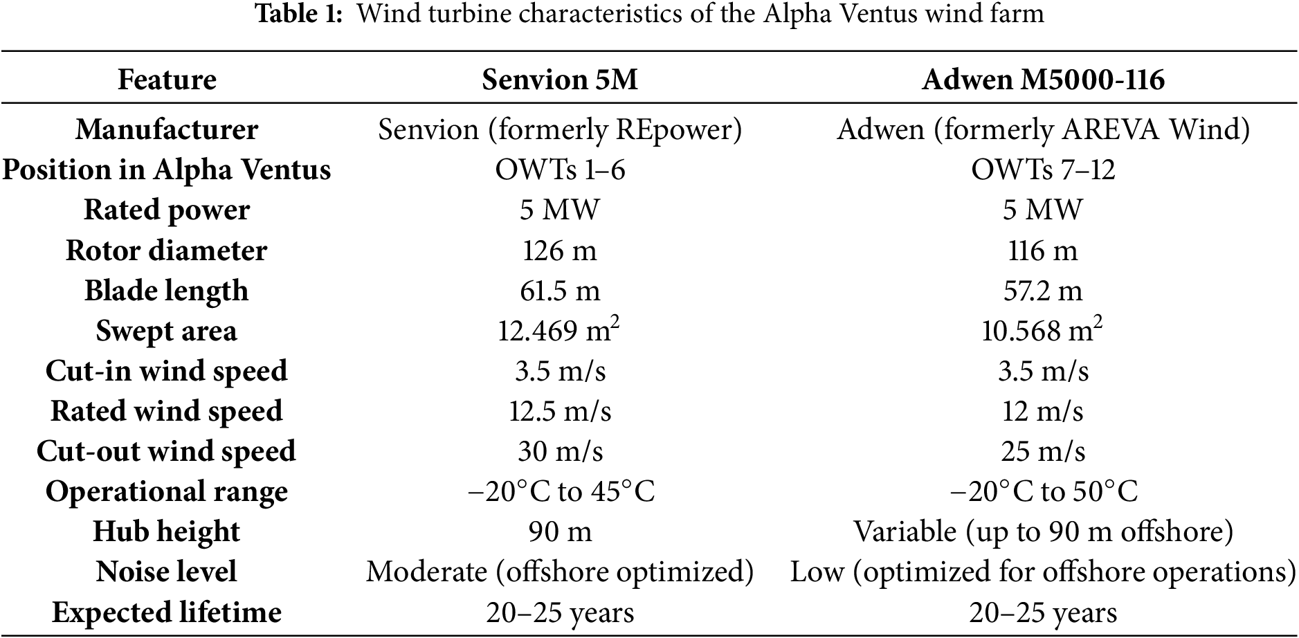
The data used in this article comes from Alpha Ventus [3] Germany’s first offshore wind farm. It is situated in the North Sea, 45 km north of the island of Borkum, at an average water depth of 28 m. This wind farm, in operation since 2010, consists of 12 turbines of 5 MW capacity each, generating a total output of 60 MW. There are two different types of wind turbines: six Senvion (now Repower) of 5 MW installed on jacket foundations, designed by Offshore Wind Energy Converter (OWEC), and six Adwen AD 5MW-116 turbines supported by tripod foundations. These turbines are arranged in a 4 × 3 grid over 4 km2, with a spacing between turbines of approximately 800 m. This spacing is designed to minimize wake effects and maximize energy capture. Table 1 shows the different types of wind turbine of the Alpha Ventus farm and the principal technical characteristics.
The wind farm includes a central offshore substation connected to the turbines via inter-array cables. In addition, the site is equipped with a meteorological mast (Met Mast F1), located approximately 403.2 m ahead of WT4. This Mast plays a vital role in collecting wind and meteorological data, contributing to accurate performance monitoring and forecasting. The precise placement of these elements is crucial for the efficient operation and management of the wind farm [33].
The Alpha Ventus wind farm has an extensive sensor network deployed across the various turbine components (on the nacelle, blades, tower). Large amounts of real-time data such as vibration frequencies, temperature fluctuations, and output power are continuously collected. Particularly, the project employs an extensive array of sensors over 1200 measurement channels distributed from the turbine foundations to the blade tips that continuously record a broad spectrum of variables. These registers include key operational parameters such as wind speed, wind direction, power output, rotor speed, blade pitch, and yaw angle, along with environmental and diagnostic data like ambient and component temperatures, vibration levels, and electrical measurements (voltage, current, frequency). Most SCADA data are logged as 10-min averages to effectively capture the dynamics of turbine performance and environmental conditions, although certain diagnostic sensors operate at higher frequencies to provide detailed transient information. With a data record spanning more than a decade, the project offers a unique long-term dataset that supports in-depth analyses of seasonal variability, turbine health, and the overall influence of harsh marine conditions on offshore wind operations [34].
Table 2 details the sensor variables, their measurement units, and associated statistical metrics used in this work.
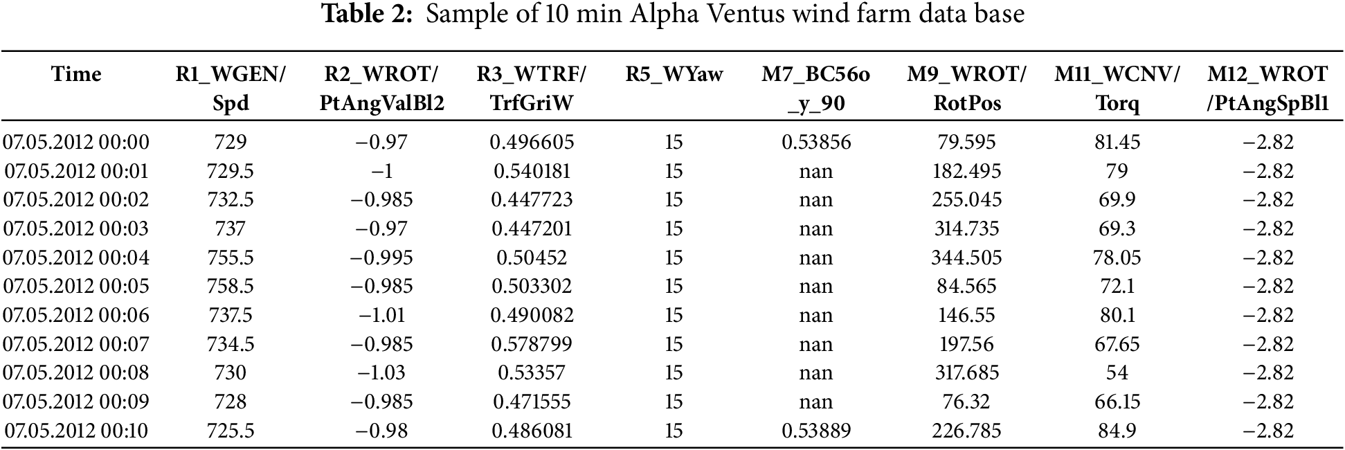
The naming convention includes both turbine type and identification number—for instance, “M7” indicates a sensor reading from turbine number 7 of the Tripod type, while “R2” denotes turbine number 2 of Jacket type. Each variable has its mean, standard deviation, minimum, and maximum values. In the example of Table 2 there are only mean values. These variables are the following. The wind generator speed (WGEN/Spd) is measured in revolutions per minute (rpm), reflecting the nacelle’s performance; the pitch angle for Blade 2 (WROT/PtAngValBl2) is expressed in degrees; it is the sme for all the blades. The transformer/grid power output (WTRF/TrfGriW) is recorded in megawatts (MW). Similarly, the yaw angle of the nacelle (WYaw) is given in degrees, the acceleration at a specific structural point (B-C56o_y_90) in meters per second squared (m/s2), and the rotor position (WROT/RotPos) in degrees. Furthermore, the torque on the converter (WCNV/Torq) is measured in kilonewton-meters (kNm), and the pitch angle speed for Blade 1 (WROT/PtAngSpBl1) is provided in degrees per second (°/s), and it is the same for the other blades.
SCADA data such as wind speed, wind direction, power output, rotor speed, and blade angles are provided continuously for all turbines, while turbines 4, 5, 7, and 8 are the only equipped with additional sensors to monitor temperature, tilt, inclination and accelerations at various points of their structures.
Fig. 1 shows the position and some variables of the turbines of the wind farm. In Fig. 1a it is possible to see the location of each of the 12 Alpha Ventus wind turbines (AV1 to AV12) of the wind farm. Fino1 is the dedicated meteorological measurement platform for this farm. AV UW (bottom right) is the undisturbed, un-waked baseline measurement point in the farm that is considered a reference. Of these, the turbines from WT1 to WT6 are Senvion type and from WT7 to WT12 are Adwen type, both currently having an age of 15 years. They were commissioned in the year 2009. Fig. 1 also shows an overview of some variables of the wind farm in the year 2016. The age of the wind farm at that time was 7 years. Fig. 1b shows the wind speed in 2016. It is possible to see how the average is around 10 m/s, near the rated speed of the wind turbines. Fig. 1c shows the total power output of the farm measured from the main power line. Fig. 1d shows the wave height during the year and how it is related to the wind speed.
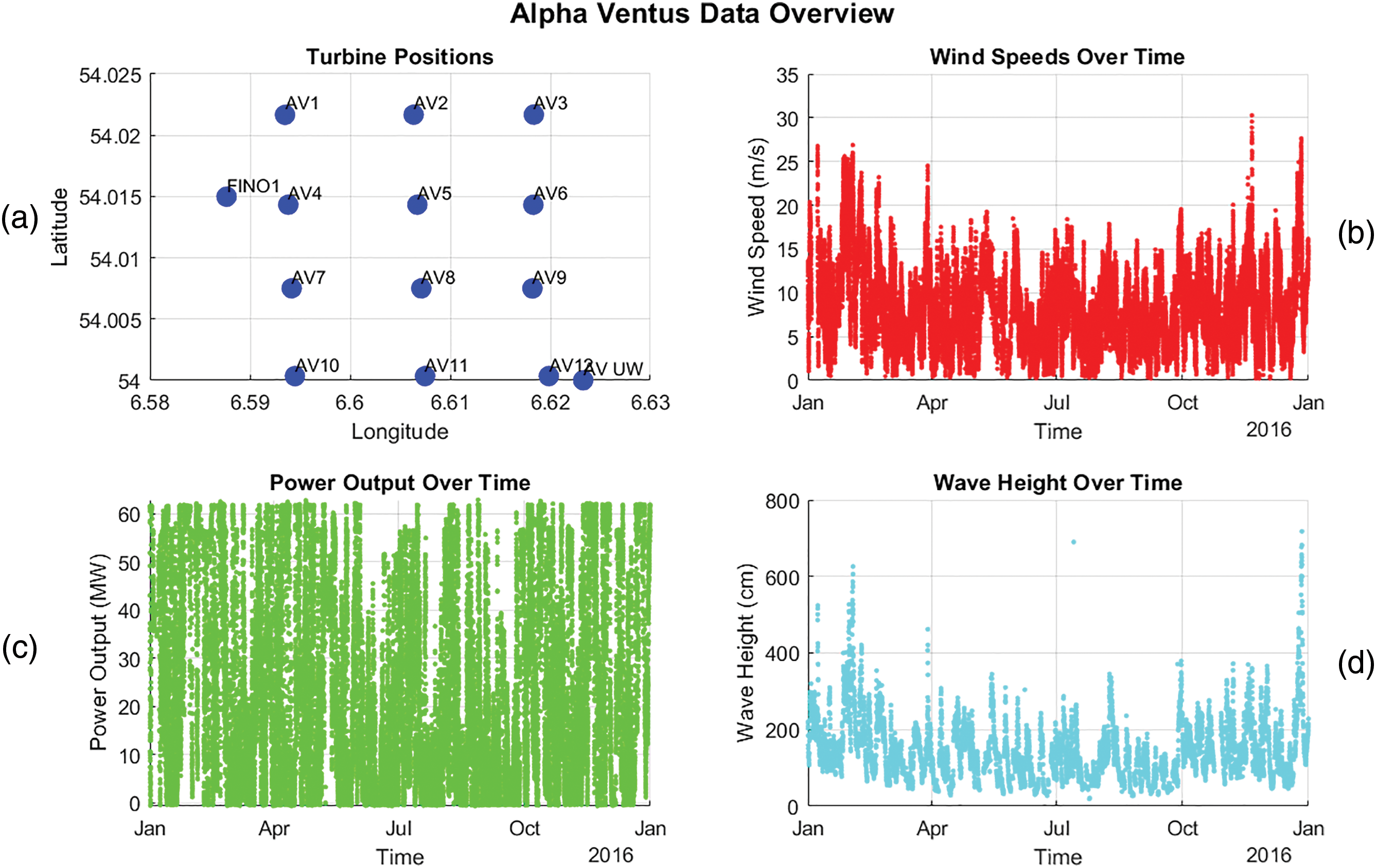
Figure 1: Alpha Ventus offshore wind farm data overview (year 2016 data). (a) Turbines Positions. (b) Farm wind speed in 2016. (c) Farm power output in 2016. (d) Farm wave height in 2016
Fig. 2 illustrates the evolution of three key operational variables—yaw error, wind speed, and power output—for turbines WT1 (Senvion) and WT7 (Adwen) during October 2016.
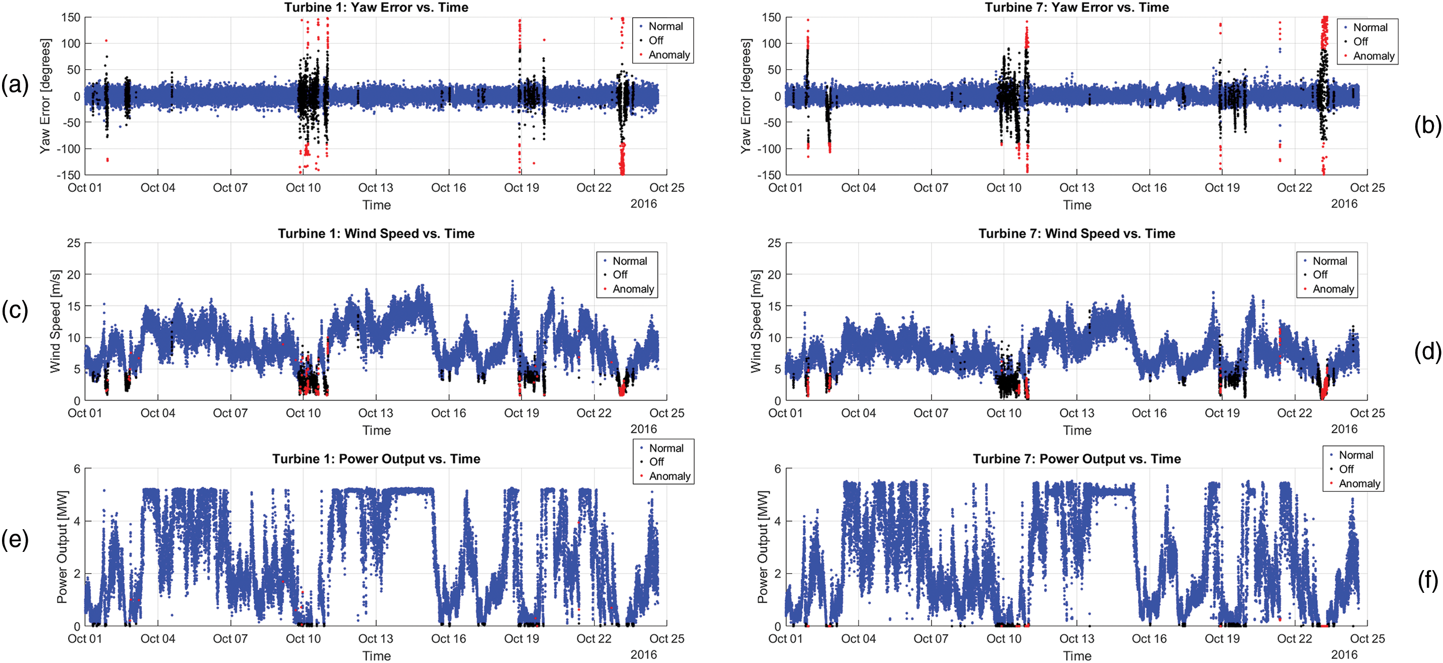
Figure 2: Some variables evolution of wind turbine WT1 and WT7 (October 2026). (a,b) compare the yaw errors. (c,d) compare the wind speed. (e,f) compare the power output
The yaw error (Fig. 2a,b) shows significant deviations, especially around October 10 and 19, likely leading to lower energy capture and increased mechanical loads. This is corroborated by the marked decrease in power output on the same dates (Fig. 2e,f), demonstrating the direct impact of yaw error on turbine performance. Furthermore, power output generally follows wind speed trends (Fig. 2c,d), as expected under normal operating conditions.
The differences in performance between WT1 and WT7 can be attributed to their respective positions within the wind farm (Fig. 1a). WT1, located at the periphery, experiences relatively undisturbed inflow, resulting in more stable wind speeds and consistent power generation. In contrast, WT7 is situated downstream of turbines WT4 and WT5, making it susceptible to wake effects. This leads to increased turbulence, higher yaw misalignment, and greater fluctuations in both wind speed and power output, ultimately reducing its efficiency compared to WT1.
The lower wind speeds observed at WT7 (Fig. 2c,d) are primarily due to its exposure to the wake generated by WT4. When the prevailing wind originates from the north or northwest, WT1 intercepts the flow first, creating a downstream wake characterized by reduced velocity and heightened turbulence. This phenomenon, well-documented in wake modelling studies (e.g., computational fluid dynamics and semi-empirical approaches), explains the diminished wind speeds at WT7’s rotor plane. Additionally, site-specific factors such as terrain-induced flow distortions and atmospheric stability conditions (e.g., thermal stratification and wind shear) may further modulate wake losses, depending on the local microclimate.
3.2 Methods: Support Vector Machines (SVM)
Machine learning algorithms can be applied to this data to detect anomalies and predict potential failures in turbine components. These models identify patterns and deviations indicative of problems such as blade erosion, gearbox malfunction, or structural instabilities.
Support Vector Machine (SVM) is a supervised machine learning algorithm used for classification and regression tasks. It works by finding the optimal hyperplane that separates data points of different classes in a high-dimensional space. The goal is to maximize the margin, which is the distance between the hyperplane and the nearest data points from each class, known as support vectors [35]. This hyperplane can be defined as a decision boundary that separates the data. For a binary classification problem, it can be expressed as:
where
The margin to be maximized is calculated as the distance between the hyperplane and the closest data points (support vectors). The margin is given by:
maximizing the margin is equivalent to minimizing
To obtain that margin, SVM solves the following constrained optimization problem:
Subject to:
where
For non-linearly separable data, a soft margin is introduced using slack variables
Subject to:
where C is a regularization parameter that controls the trade-off between maximizing the margin and minimizing classification errors.
The most important part of the application of SVM is selecting a kernel function to map input data into a higher-dimensional space. Common kernels include:
Linear:
Polynomial:
Radial Basis Function (RBF):
The configuration of the SVM parameters was determined through an in-depth evaluation process. The Gaussian Radial Basis Function (RBF) is used here as a kernel for the SVM, leveraging MATLAB’s built-in fitcsvm implementation. Although fitcsvm provides robust defaults, these settings are validated on October 2016 subset of the Alpha Ventus SCADA data, using 5-fold cross-validation to ensure optimal generalization. This process confirmed that a regularization parameter C = 1.0 (with the default kernel scale) achieves the best trade-off between margin maximization and misclassification control. Once trained, the same SVM framework applies for different types of turbines and locations.
This paper attempts to classify the source of the anomalies. To do so, the following possible states or anomalies associated with the operation of wind turbines are considered.
• Stopping: is a controlled stop and securing of the rotor, to avoid involuntary movements, especially during maintenance, extreme weather conditions or grid failures. It is not considered a failure since stopping the rotor ensures the safety of the turbine, reduces wear and protects components from damage in strong winds.
• Power reduction: can be intentional, to improve longevity, improve grid stability, reduce noise or comply with regulations. But it can also be an indication of a failure or an anomaly in some component of the turbine or in the sensors.
• Environmental factors: which can affect the performance, efficiency and life of turbine components. For example, ice build-up on the blades reduces efficiency, but there is no data on this type of failure in the database being worked with.
• Wakes: When wind passes through a turbine, it slows down and becomes turbulent, creating a wake that affects downstream turbines, leading to lower efficiency and higher fatigue loads on nearby turbines. This effect will be studied and can be identified in the turbines discussed in this article.
• Sensors: Wind speed, direction, temperature, vibration and blade position. These sensor failures or inaccuracies can lead to suboptimal power generation, increased wear or even turbine shutdown. Failures in power measurement not only lead to inaccurate power readings and financial losses but also hinder the detection of inefficiencies.
• Communication equipment errors: These can occur due to signal interference, hardware failures, software failures or environmental factors such as lightning or extreme weather conditions. These problems can disrupt remote monitoring and control, leading to maintenance delays and lower efficiency.
Those six cases of anomalies or faults are reflected in one way or another in the data available in the wind farm database, specifically in the power curve of the wind turbine, and an attempt will be made to detect some of them. In some of those cases they will appear as power anomaly because there is enough wind but no power output. Stopping will be ignored because also it is easy to detect using the power curve.
The power curve of a wind turbine shows the relationship between wind speed and power output (Fig. 3).
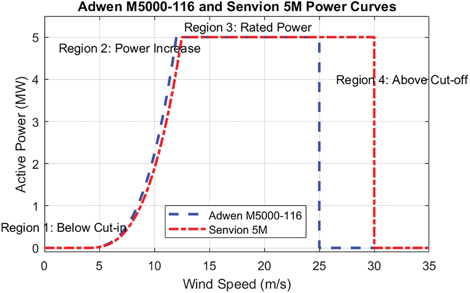
Figure 3: Ideal operation regions of Adwen (blue line) and Senvion (red line) wind turbines
It typically follows a pattern where below the cut-in wind speed (region I), no power is generated. As the wind speed increases and exceeds the cut-in threshold, the turbine starts generating power and output increases rapidly following cubic growth (region II). Once the rated wind speed is reached, power output stabilizes at the maximum rated capacity of the turbine, ensuring safe operation (region III). Beyond the cut-off speed, the turbine shuts down to prevent structural damage from excessive forces (region IV). That is, the turbine operates following these operational modes, all of them controlled by robust systems to maintain optimal performance and safety. Fig. 3 shows the wind speed values that define these operating regions for the two specific types of turbines in the wind farm.
In region II, where output power increases, the power is proportional to the cube of the wind speed according to Eq. (8).
where:
•
•
•
•
To illustrate this relationship between wind speed and power output from real data, Fig. 4 shows the actual power curves for wind turbine WT1 and wind turbine WT7, both from different manufacturers and situated at very different positions on the farm, highlighting the differences in performance.
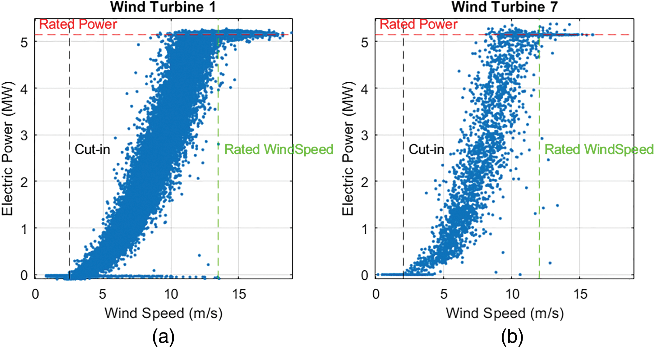
Figure 4: (a) Power curve of Adwen (WT1) and (b) Senvion (WT7) wind turbine
As can be seen in Fig. 4, both turbines exhibit a power curve that fits the typical expected profile, where power output increases as wind speed increases, reaching a plateau at rated power. WT1 shows a smoother power curve, reaching rated power (~5 MW) at approximately 12 m/s corresponding to the rated speed, and maintaining it steadily. However, WT7 reaches rated power at around 10 m/s, but shows a significant dispersion in its output power, particularly at mid-range wind speeds (6–10 m/s), suggesting a higher variability in its performance. This dispersion could indicate wake factors, mechanical inefficiencies, suboptimal control strategies or environmental influences that affect that WT7 turbine more.
Model Identification
To identify a model of the wind turbine power curve, the choice of the degree of the polynomial is important as it affects the accuracy of the model. A comparative analysis of the fit of the data to the non-linear models of third degree (cubic), the theoretical one given by Eq. (8), and of second degree (quadratic) reveals notable differences in that fit. However, according to Eq. (8), if the power were represented as a function of the cube of the effective wind speed, an almost linear behavior should be obtained.
That is, due to aerodynamic inefficiencies, disturbances and inaccuracies of the control system, in real systems the curve of the measured power data of the turbine as a function of wind speed fits better to a quadratic function than to a cubic one, as shown in Fig. 5.
Fig. 5 shows a linear fitting with respect to the cubic and squared wind speed.
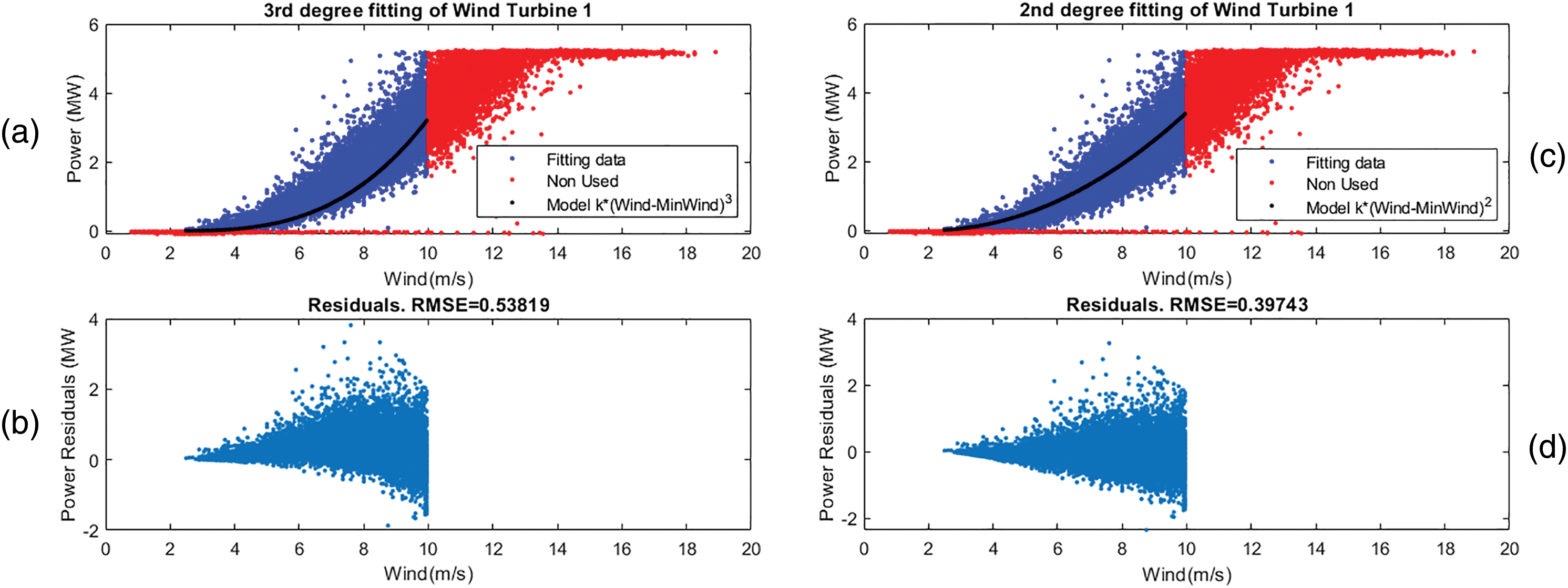
Figure 5: (a,b) 3rd degree fitting; (c,d) 2nd degree fitting
The selection of a second-order polynomial fit (Fig. 5c) over a third-order one (Fig. 5a) is based on the behavior of the residuals and the physical interpretation of the data. When fitting a model, the residuals—defined as the difference between the observed values and the model predictions—are a key diagnostic tool. If the residuals exhibit systematic patterns or curvature, it typically indicates that the model is not well-suited to the data, either due to an inappropriate choice of degree or base. The residuals from a third-order polynomial fit (Fig. 5b) exhibited a clear curvature, suggesting overfitting or the introduction of unnecessary complexity. In contrast, a second-order polynomial (Fig. 5c) resulted in residuals that were randomly distributed without curvature, which is a strong indication of an appropriate model choice. Residuals reduce their displacement and curvature, and for that reason the resulting RMSE is significantly better, 0.39 compared to 0.53.
One contributing factor is that the performance of real wind turbines, particularly those nearing the end of their operational life, is generally lower than that predicted by idealized models. Moreover, wind speed measurements are typically acquired from anemometers mounted on the nacelle, where the airflow has already been altered by the turbine structure. Consequently, the recorded wind speed does not accurately represent the undisturbed incoming wind that actually drives the turbine. This discrepancy can lead to deviations from the ideal power curve, which may be more accurately captured using a lower-order polynomial model.
This result is significant because it challenges the assumption—common in the literature—that third-order polynomial necessarily provides better fit for wind turbine power curves. This research findings, based on real operational data from two different wind turbines, suggest that a second-order polynomial better captures the actual behavior of these real systems. This observation aligns with [16], where other bases are proposed to offer a more reliable and efficient representation of the wind turbine power curve.
This means that, according to the experimental data, the extracted power is behaving as a system proportional to the square of the wind speed. Therefore, for anomaly detection a second-degree model of the power curve will be used. It includes the dead zone and power saturation regions, and can be expressed as:
where the first factor models the region where there is not enough wind to start the turbine. When the wind speed is less than or equal to the cut-in speed, this factor is 0; otherwise, it is 1. The min function saturates the model power to its maximum for wind speed values above the rated speed.
5.1 Data Analysis of Input and Output Variables
Before applying machine learning techniques to detect anomalies, a visual analysis of the data has been carried out to extract some information that can help identify the type of anomaly or the source of these failures.
The turbines have been analyzed according to their type and age. That is, turbines WT1–WT6 are of type Senvion and Turbines WT7–WT12 are of brand Adwen. The turbines were installed between July and November 2009. The entire wind farm became fully operational in April 2010. The data used in this research is from 2016. The age of the turbines in the time of the study is 6 years. In addition, their position on the farm was shown in Fig. 1a.
The input variable wind speed is measured in the nacelle by an anemometer sensor, which is located behind the rotor, so the measurement is distorted by the wind turbine itself since the wind has passed through the blades. In addition, the wind measurement system is different for each type of wind turbine on the farm. To analyze how this measurement is affected, the value of this turbine sensor is compared with the wind speed measurement at the station; the difference has been called measurement wind speed error. Fig. 6 shows mean and standard deviation (std) of this error for both types of wind turbines.
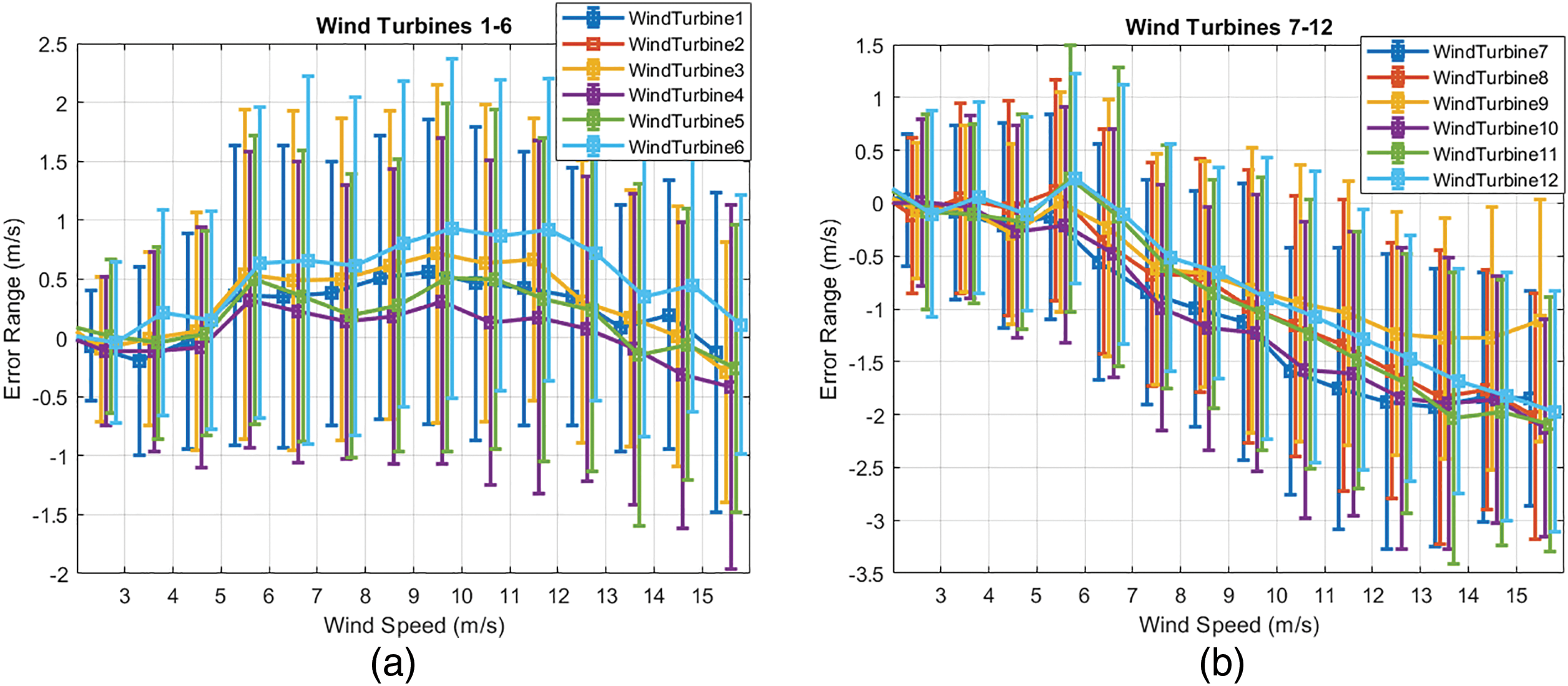
Figure 6: (a) Measured wind speed error at WT1–6; (b) Measured wind speed error at WT7–12
As can be seen in Fig. 6, when the wind is more aggressive, the error is greater than if the wind is light. This greater error in the measurement of high-speed winds is not worrying, because in the case of high-speed winds the power of the wind turbine is limited by the control system. It can be concluded that, for the WT1–6 wind turbines in the operating wind speed range [3, 10] m/s, the mean error is negligible, and the standard deviation is more or less constant, around 1 m/s. However, for the WT7–12 turbines, the mean error and the standard deviation increase with speed, although for low-speed winds the standard deviation is similar to that of WT1–6. This analysis will help identify and eliminate potential errors.
The same has been done for the other variable that provides information on the operation of the turbine. The output power error of the wind turbine must be estimated in the nominal power zone. In this zone the wind is strong (overrated) and therefore the wind speed error does not significantly influence the power. That is, the error in this case will be mainly due to errors in the power control system and in the measurement sensors. Fig. 7 shows the typical deviation of the power error in the nominal region for both types of wind turbines.
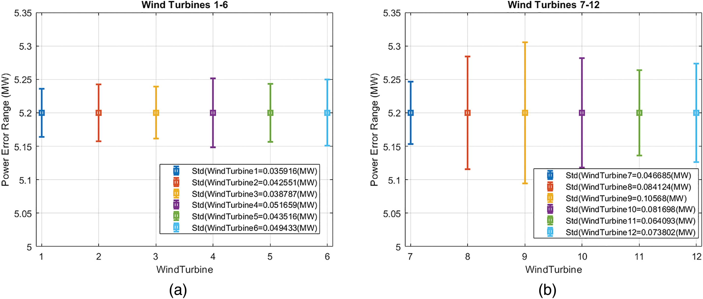
Figure 7: (a) Output power error of WT1–6; (b) Output power error of WT7–12
It can be observed that the std of the power is not significant, less than 0.05 MW for WT1–6 and smaller than 0.1 MW for WT7–12.
5.2 Anomaly Classification Based on Confidence Intervals
As shown in Fig. 4, the measured power curve data can be very noisy. This may be due to system failures or inefficiencies, and/or to failures or inaccuracies in the measurement of the input (wind) and the output (power) of the wind converter. Since the input and output measurement errors have been previously characterized, these errors can be included in the model to obtain confidence margins for the anomaly detection system. The output errors must be added to the output of the model, and the input errors must be propagated through the power curve model. For instance, equations of the positive and negative limits for a 95% (
where
The model of the power curve (black line), the real data (blue dots), and confidence intervals of 68% (
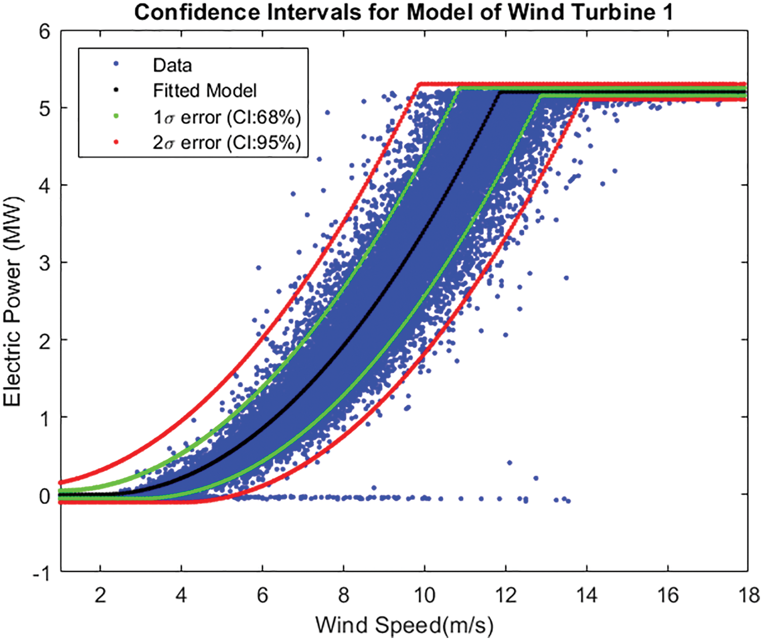
Figure 8: Confidence margins
Using these confidence intervals, it is easy to make a basic classification of anomalies. Values within the confidence interval are considered as nominal (normal) behavior, values above the upper limit are considered as wind measurement anomaly, and values below the lower limit are classified as power anomaly.
Using the second order power curve degree model and confidence margin, the detection of both types of anomalies over time is shown in Fig. 9.
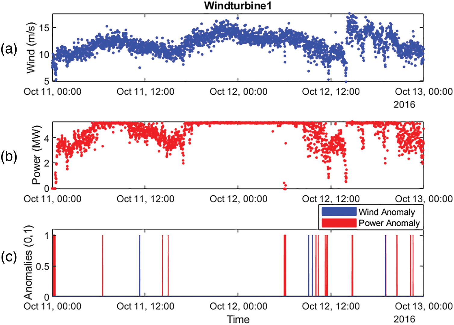
Figure 9: (a) Wind speed, 10, (b) power, and (c) anomalies at days 11 & 12 October 2016 in WT1
The results show the temporal relationship between wind speed and power output of the WT1 turbine. The top graph shows the wind speed fluctuating between 5 and 15 m/s for two days, 11 and 12 October 2016, while the middle graph shows the power output, which is generally correlated with wind speed but includes fluctuations and possible interruptions. The bottom graph shows the anomalies, with blue lines indicating wind anomalies and red lines marking power anomalies.
5.3 Data Linearization and Normalization
Data-driven detection and identification techniques are highly dependent on the information provided to them. They are often designed for specific problems, so the configuration is ad hoc. However, it would be highly desirable if the effort to select a technique, configure it, and apply it to data, which is generalizable and applicable to a wide range of conditions and systems. To make the methodology general, a normalization process is proposed and developed in this work. Normalization is important in this research as it ensures that wind speed (measured in m/s) and power (measured in MW), which operate at different scales, can be compared in a consistent manner. By standardizing these variables, anomalies can be detected more effectively and fairly, as it prevents the larger scale of power data from overshadowing small variations in wind speed data.
In addition, normalization facilitates consistent detection of anomalies across different turbines and sensor configurations within the wind farm, allowing for robust and reliable analysis of wind farm performance. In this case, regarding the power curve, considering the squared wind speed as input, the power signal would be a linear function. Furthermore, by working with normalized values around the key points of the power curve, no model is required. Therefore, the following normalization of the variables of the wind turbine power curve is proposed. The Normalized Wind Speed (WSn) can be defined as:
where:
• v: The actual wind speed at a given moment (m/s).
•
•
In the same way, the Normalized Electric Power (EPn) is defined as,
where:
•
•
During signal normalization, only a lower bound of zero was applied, while the upper bound was intentionally left unrestricted. This approach allows high-magnitude noise and outliers to propagate through the processing chain without being truncated prematurely. These values will then be evaluated and constrained using the adaptive margin bounds defined in Eqs. (16) and (17). With these normalized signals, the power curve transforms into a saturated linear function with slope 1. Fig. 10a (top graph) shows the new power model for WT1 when the wind speed and output power variables are normalized.
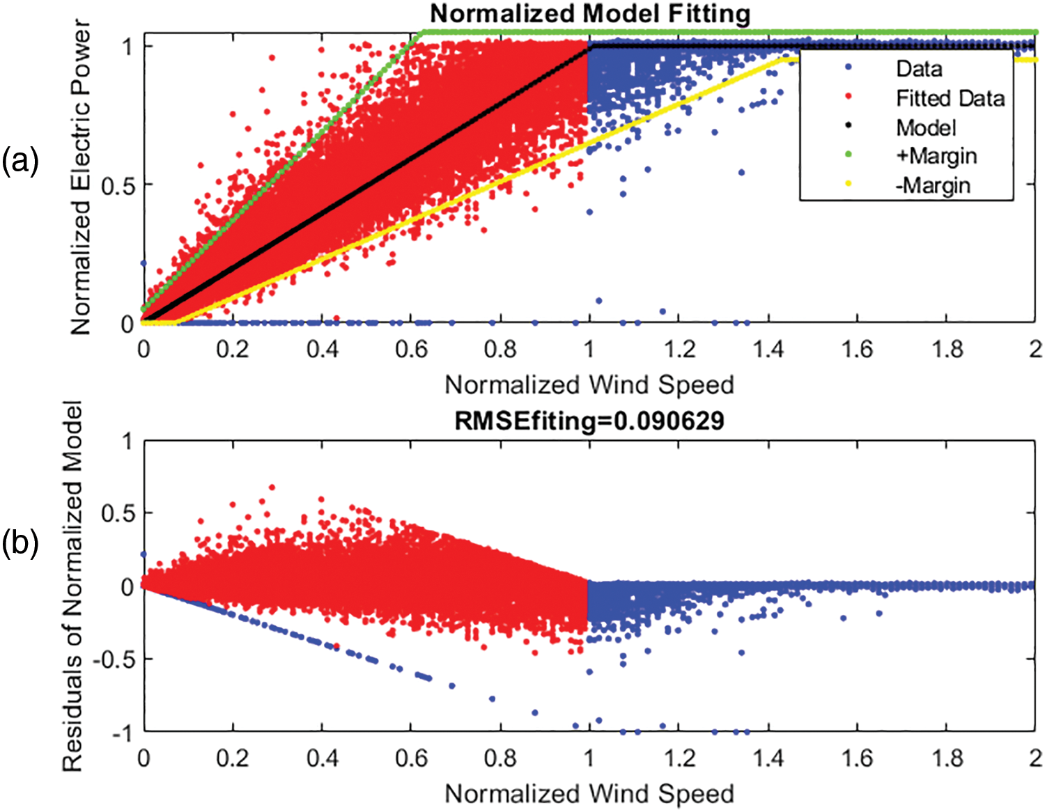
Figure 10: WT1 model fitting, (a) Normalized Power; (b) Residuals
The model follows the linear function represented by the (black line). The positive (green) and negative (yellow) lines indicate error margins, formulated in Eqs. (16) and (17). These error margins can be fitted to provide margins of confidence too. Fig. 10b (bottom graph) shows the residuals of the model fit and its RMSE, which in this case is quite small (0.0906). It is important to note that in the transient zone the error margins are proportional to the normalized wind, while in the nominal zone the error is the normalized power error.
Using these normalized signals is possible to define the Wind to Power Index WPi, described in Eq. (18). This linear index indicates how close the real output power to the ideal power curve is. In this index, the normalized wind speed is saturated to consider the region where the output power stays at its maximum value by the control system of the wind turbine.
The index can be interpreted as follows:
• A value of 0 indicates ideal theoretical operation.
• A value greater than 0 means that more power is being generated than the estimated from the measured wind speed. This suggests that there may be an anomaly in the wind measurement.
• A value less than 0 means that less power is being generated than the estimated from the measured wind speed. This suggests that there may be an anomaly in the generated power.
Fig. 11 shows the behavior of this index, which is a function of the two normalized variables of the wind turbine power curve.
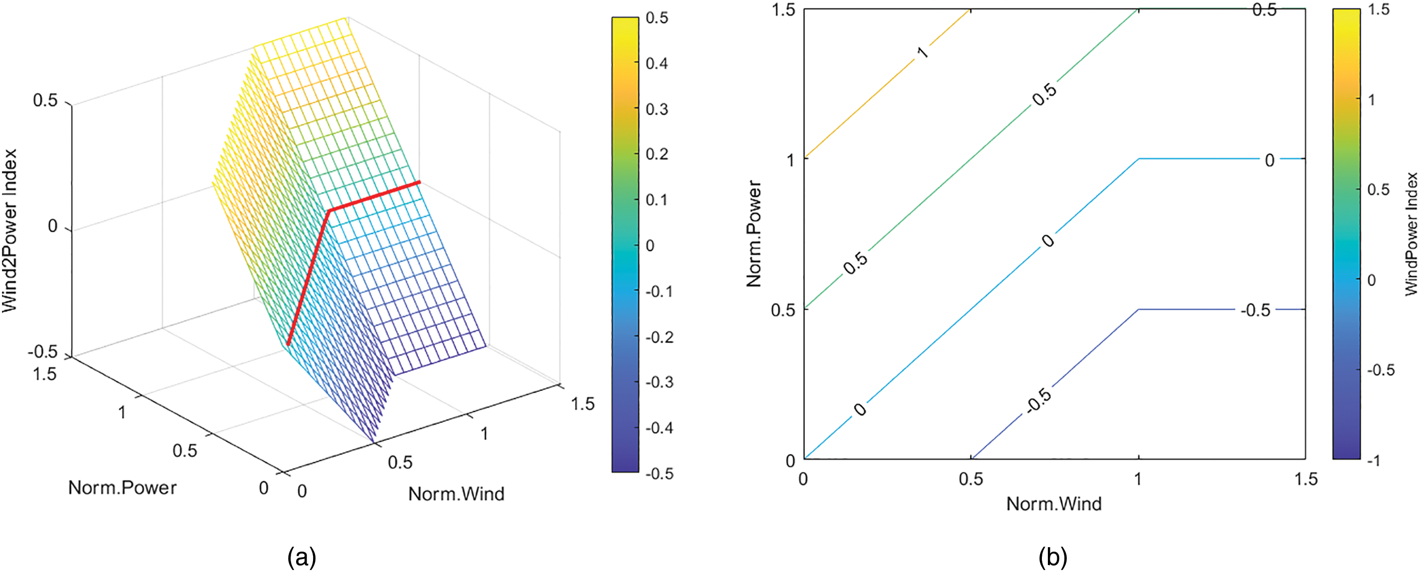
Figure 11: (a) Ideal index surface; (b) Index contour curves (right)
In Fig. 11a, the red line shows the ideal behavior, with WPi index equals to zero. There are two planes, one representing the behavior of the index when the turbine is working at nominal speed, and another when it is working with under rated winds. Fig. 11b shows the contour lines of the index surface.
In addition, the value of this index indicates the extent of the anomaly. Using this approach, the error margins can be projected onto the power index surface and thus used to classify the anomalies. Fig. 12 shows the anomaly classification of the WT1 wind turbine data using the Wind Power Index (WPi) Eq. (18) and the error margins described in Eqs. (16) and (17).
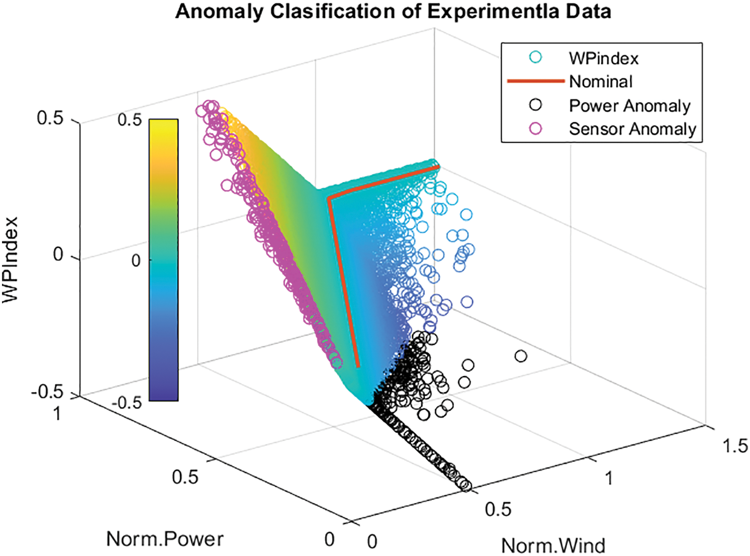
Figure 12: Anomaly classification of WT1 output power data
In Fig. 12, the axes represent normalized power, normalized wind, and the WPi index, which serves as an indicator of wind turbine performance. Black and pink circles are used to point out an anomalous performance, according to the defined margin errors. The pink points are sensor anomalies, due to sensor inaccuracies, turbulence, or external environmental disturbances. The black points are power anomalies, possibly caused by mechanical inefficiencies, transmission problems, or control system failures. The color bars codification is used to evaluate the wind turbine performance in a progressive way. Green circles are used where power output aligns with wind conditions, clustered around the WPi ≈ 0 shown as a red line. The yellow circles are near to wind anomalies and dark blue circles are near to power anomalies.
The introduction of this standardization helps compare the behavior of different types of turbines and analyze their behavior over time, considering their history and obtaining patterns of their temporal evolution, and in space, analyzing the coherence of the signals to see if they reflect the influence of the different locations of each turbine within a farm.
6.1 Anomaly Detection Based on Wind Porwer Index
Temporal coherence measures the correlation between system properties over time. Since the wind power index (WPi) is divided by the normalized wind speed, it is possible to isolate the temporal analysis from the excitation conditions at the turbine. Long-term coherence is implicit when calculating the wind power index,
• Those indicated in the manufacturer’s specifications (
• Experimentally readjusted during the commissioning phase (
• Updated after major maintenance or repair (
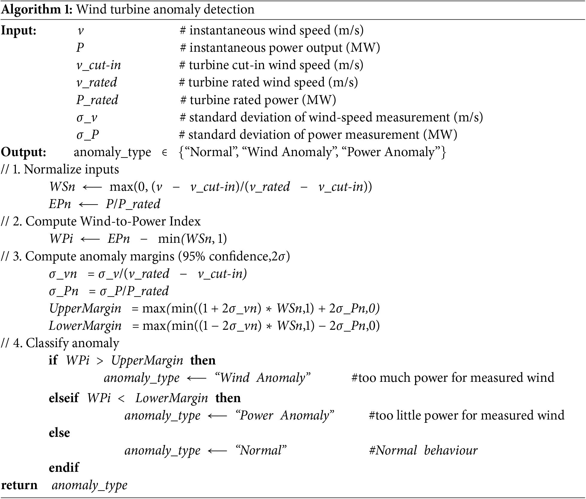
Using normalized signals, the index allows wind turbine operators to directly diagnose deviations from expected performance, identifying whether the problems are due to inconsistencies in wind measurement or to power anomalies generated by the wind turbine. Algorithm 1 describes the steps of the anomaly detection methodology. This algorithm is applied during operation to each data sample provided in real time by each wind turbine.
Using Algorithm 1, an analysis of the WT1 signals is shown in Fig. 13.
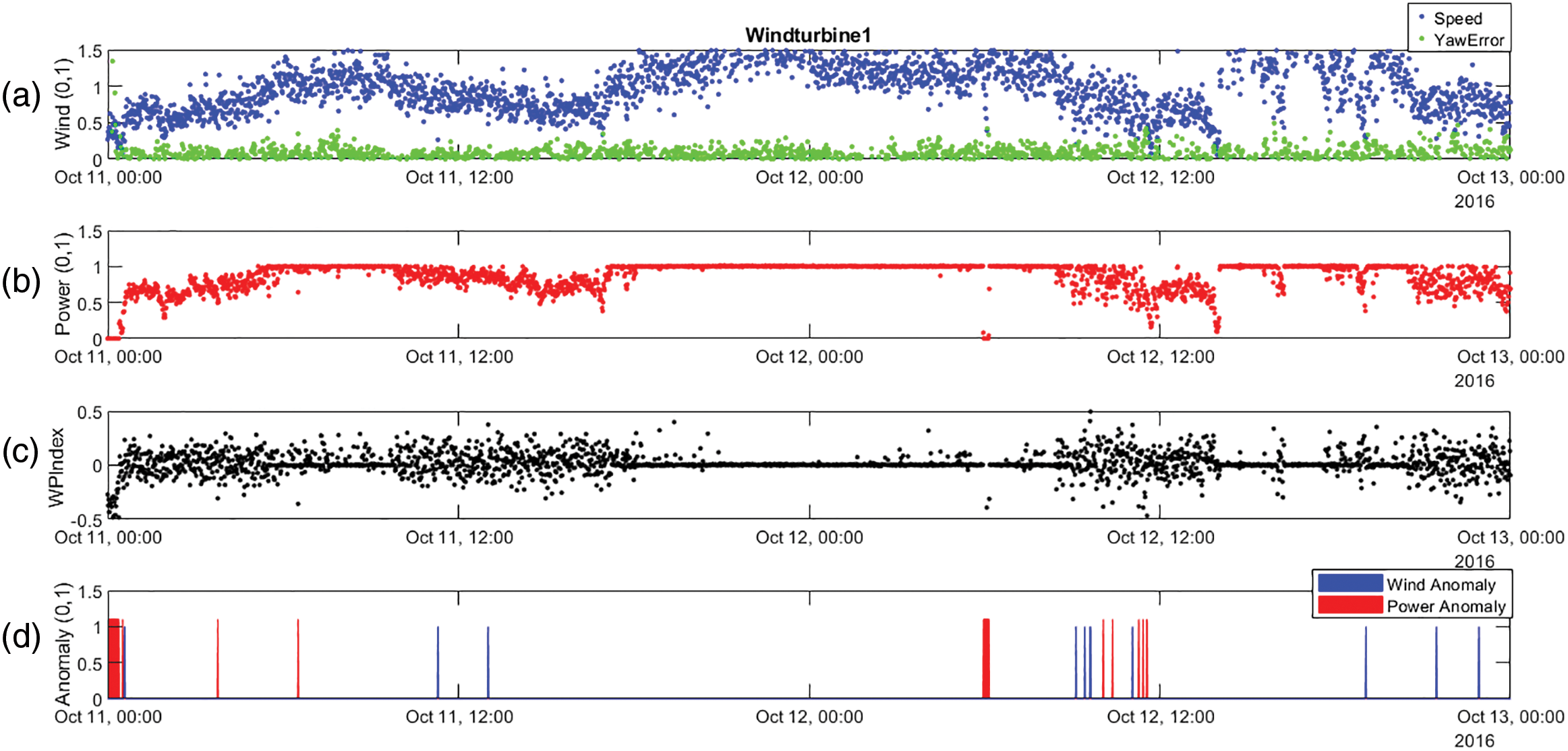
Figure 13: From top to bottom, (a) Normalized wind speed and yaw error, (b) Normalized power, (c) Wind to power index, and (d) Anomalies detection for WT1
As can be seen, the results shown in Fig. 13 are very similar to those obtained previously using the confidence margins of the non-normalized power curve. However, some cases of power drop are not considered an anomaly because they are accompanied by a drop in wind speed. This is consistent, because in low wind situations, low power generation is a normal situation.
Applying the same indices and thresholds also yields good results for WT7 (Fig. 14). This proves that this anomaly detection method can be used for different turbine models. Furthermore, this methodology does not need to identify the model of the power curve, it only requires the parameters used in normalization and indices.
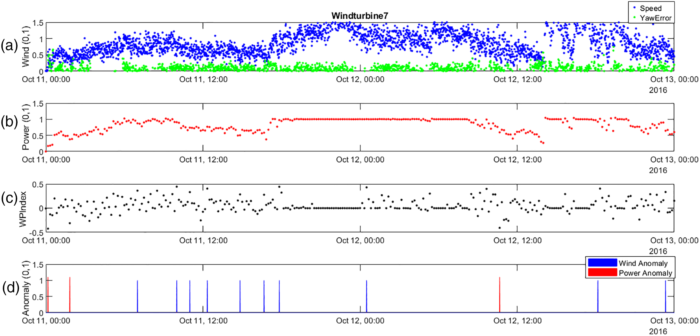
Figure 14: From top to bottom, (a) Normalized Wind speed and yaw error, (b) Normalized Power, (c) Wind to Power Index, and (d) Anomalies detection for WT7
Fig. 14 shows the performance of WT7 between 11 and 13 October 2016. A good anomaly classification has also been obtained for WT7, which is a different brand than WT1, using the same error margin limits (that is, the P ± margins of WT1). Both offshore wind turbines operated under the same wind conditions, but with different performances. WT7 produced consistently stable power (around 0.9–1.0), while WT1 showed more fluctuations in power output. Although WT7 recorded more wind anomalies (suggesting greater sensitivity to turbulence), WT1 experienced more power failures, indicating potential inefficiencies. These differences are likely due to design factors such as rotor size, control systems, and age, with WT7 being a newer model offering more precise pitch and yaw control. This type of turbine, the Adwen group to which WT7 belongs, is more efficient and makes better use of the wind, so there are fewer power anomalies. On the other hand, there are more wind anomalies, because the wind speed measurement suffers more disturbances in this type of turbine. Therefore, according to the previous analysis, for this type of turbine the upper error margin limit of the wind power index should be high.
Fig. 15 shows the performance of WT4 between 11 and 13 October 2016.
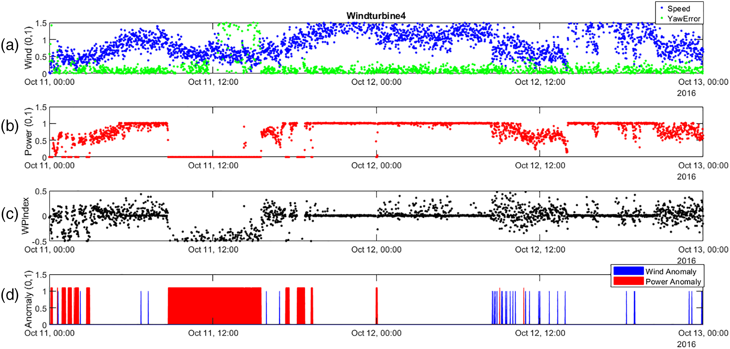
Figure 15: From top to bottom, (a) Normalized wind speed and yaw error, (b) Normalized power, (c) Wind to power index, and (d) Anomalies detection for WT4
In the case of WT4, faults are continuously being detected, as it can be seen in the anomaly graph. This even generated total stoppages in energy production for long periods of time, as can be seen on 11 October. In the following days, maintenance work had to be done on this turbine. By training the SVM on normalized variables (WSn, EPn, and WPi), the model effectively distinguishes between subtle variations in turbine performance that are often masked by measurement noise.
6.2 Anomalies Classification with SVM
Dealing with normalized signals and normalized indices has also other advantages such as:
• This normalization facilitates the physical interpretation of the signals and indices. It is also independent of the wind turbine model and thus, it is possible to merge information from different types of wind turbines.
• It is possible to define logical rules that allow refining the detection and classification of anomalies. For example, conditions such as for wind speeds lower than 20% of the nominal wind and power generation less than 50% of nominal power… A combination of the above conditions can be formulated as (WSn > 0.2) & (EPn < 0.5).
• The Wind to Power Index, WPi, can also be interpreted as a deviation from the expected efficiency in the wind turbine, so efficiency limits could be included in the logical rules. For example, WPi > −0.2 means that the efficiency is greater than 80% = (1 − WPi) ∗ 100.
Using rules based on percentages of normalized signals, anomalies can be classified for the different modes of operation. Table 3 shows the logical rules used to classify faulty operational mode according to normalized signals levels.
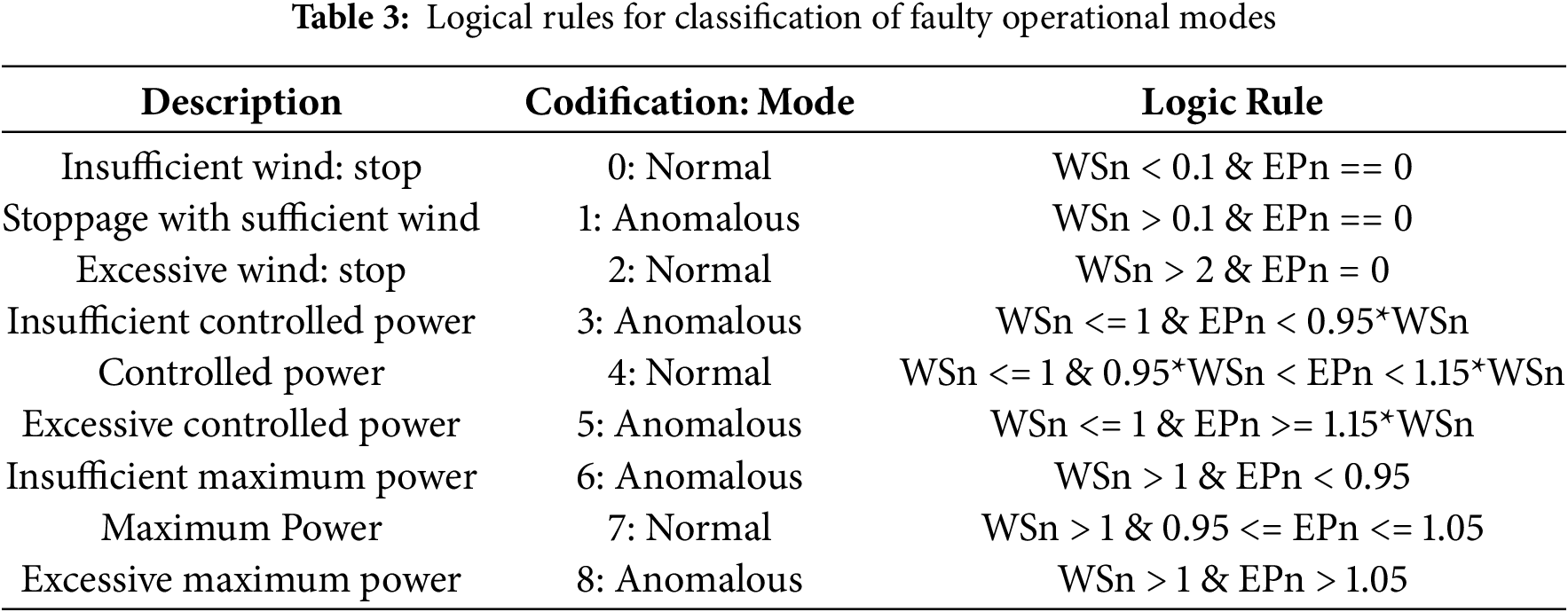
The application of these rules allows the automatic classification of experimental data in normal or faulty operational modes, as it is shown in Fig. 16.
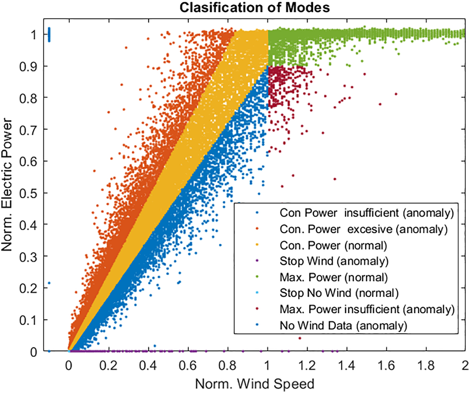
Figure 16: Rules-based classification of modes and anomalies
From this rules-based classification, a machine learning model has been trained using the Support Vector Machine (SVM) algorithm, where the input variables are WSn, EPn and WPi. Validating the trained model yields the following confusion matrix, shown in Fig. 17. The rules-based classification is shown in rows, and the classification by the SVM model in columns. The matrix is clearly diagonal dominant, as expected. Even so, there are some cases of validation that classify them differently, cases that it is convenient to analyse:
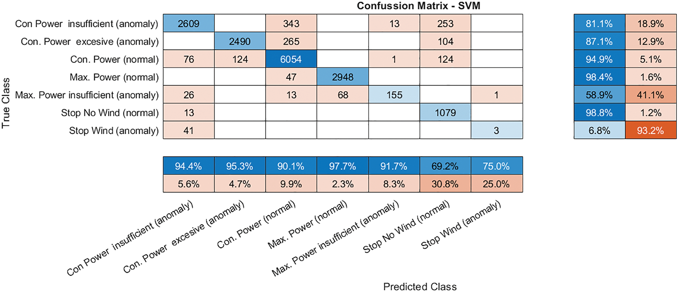
Figure 17: Confusion matrix of SVM validation
• Both in “Con. Power Insufficient (anomaly)” and in “Con. Power Excess (anomaly)” a percentage of points are classified in border areas. A large part of these cases is considered “Stop No Wind” because the wind is practically null. Another part has been considered as “Con. Power (normal)”, which is a border area that can be entered due to errors in the wind measurement.
• “Con. Power (normal)” and “Max Power (normal)” are very well classified.
• On the other hand, the “Max Power insufficient (anomaly)” is misclassified 41% of the time towards frontier values. This makes sense, because analysing the trend of the points, it can be seen that a large part of the pre-classified points in this area really follows a trend of previous areas.
• Stops due to lack of wind are classified correctly, while stops with wind are often classified as “Con. Power Insufficient (anomaly)”, because they generate some power.
The SVM classification presents a more uncertain response than the pre-classification carried out by rules. In reality, due to perturbations and measurement errors, the boundaries are not perfect, and the behaviour is fuzzy, as the SVM model behaves. In addition, the model captures the trend of points in the underpowered anomalous zone, even better than strict rules. Fig. 18 shows a real time classification made by the SVM model during the day of October 11. The WT4 has been chosen because it presented anomalous behaviour during these dates.
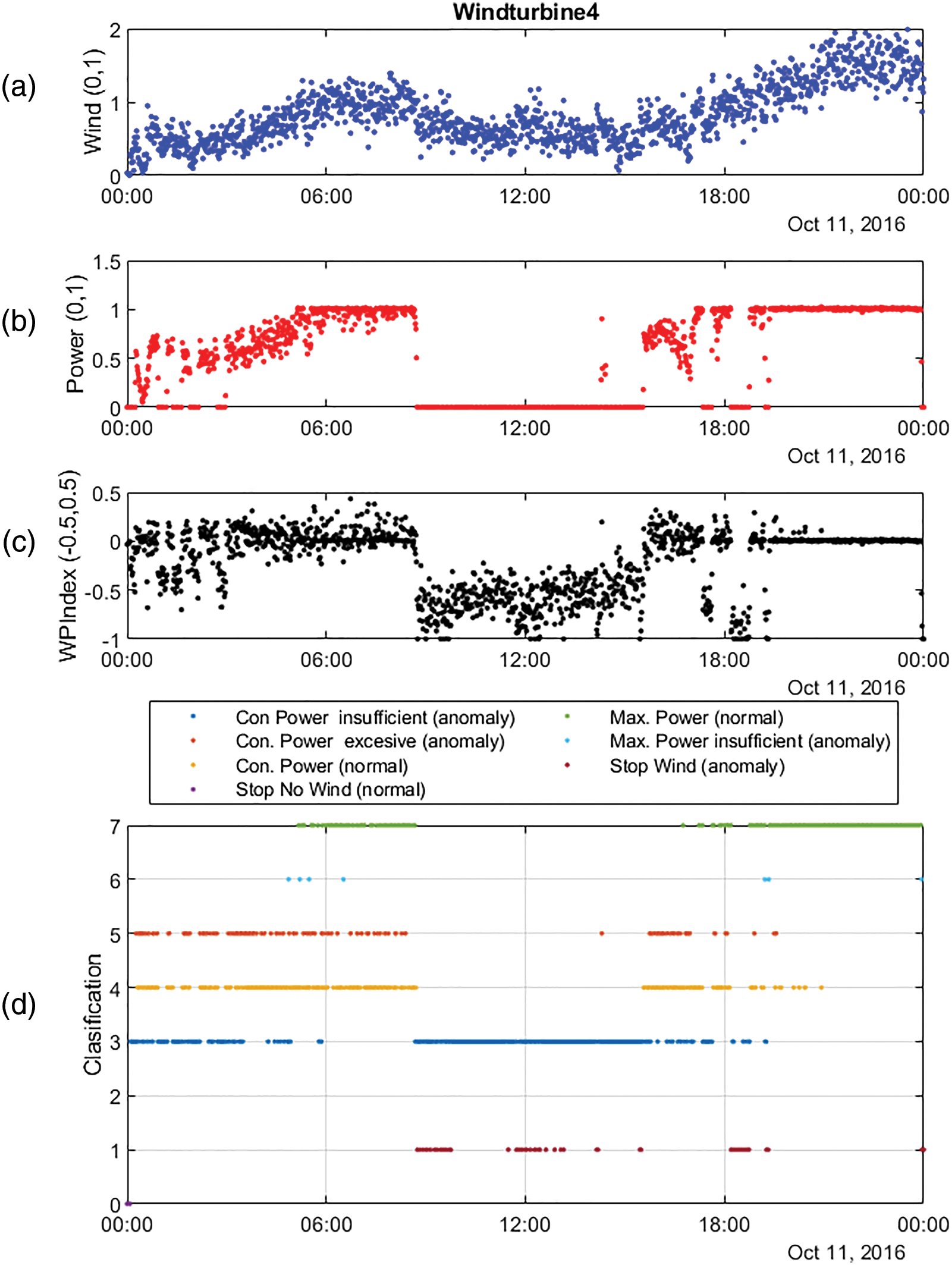
Figure 18: From top to bottom, (a) Normalized Wind Speed, (b) Normalized Power, (c) Wind to Power Index, and (d) Anomalies classification for WT4
In Fig. 18, only at the beginning, a stop occurs due to lack of wind (classified as 0). When the winds are strong, WT4 works correctly with normal behaviour (7) and few insufficient power anomalous cases (6). On the other hand, with poor winds, normal behaviour (4) alternates with quite a lot of anomalous behaviour, insufficient power (3) and excessive power (5). In addition, in the central area of the day there are anomalous stops (1) although there is enough wind to operate in controlled mode.
6.3 Spatial Coherence Analysis
Spatial coherence describes the correlation between the properties of a system at different spatial points. In this case, spatial coherence can be assessed by comparing signals and indices from wind turbines subjected to similar conditions over a time interval. For example, wind turbine j can be graphically compared with wind turbine k over the time interval
This stipulated time interval,
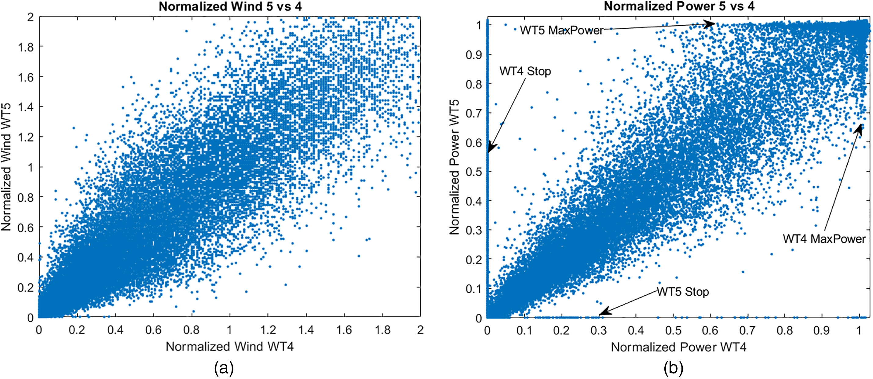
Figure 19: WT5 vs. WT4 spatial coherence, (a) Normalized wind and (b) Normalized power
In the wind graph comparation (Fig. 19a), no significant asymmetry is observed with respect to the main diagonal, which is the ideal situation. This means that the wind record is similar for both wind turbines, WT4 and WT5, so they show spatial coherence. In the power graph comparation (Fig. 19b), only a little asymmetry is observed with respect to the main diagonal, so they still show good spatial coherence. WT4 has many points in the zero-power zone, meaning it stops many more times than WT5. It is also observed that wind turbine WT5 reaches the maximum power zone more times than WT4.
Fig. 20 shows the comparison of the WPi indices of turbines WT5 and WT4 over a month. Ideally, both indices should be zero, as the wind turbines operate in nominal mode, where the error in wind speed is not relevant and the error in power should be very small. In the nominal zone the error margin is the power error, shown in red in the figure. But in the other operation zone the error margin is a function of wind speed. For this reason, Fig. 20 shows the maximum error margins vs. the normalized wind speed, described in Eqs. (20) and (21). That is, the maximum errors are defined as the maximum of the difference between margin and model.
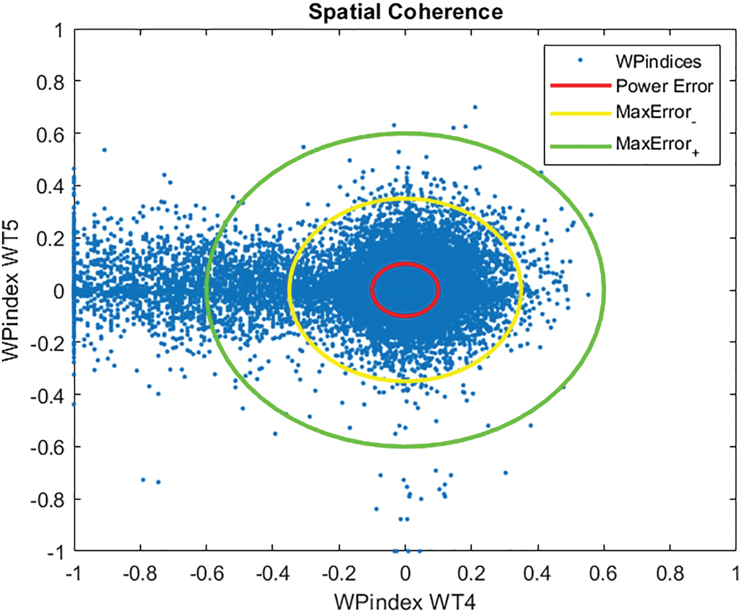
Figure 20: WT5 vs. WT4 Wind-Power Indices spatial coherence
Fig. 20 shows that many points are beyond the maximum errors’ limits. Most of these points are in the zone where WPindex4 is negative and WPindex5 is close to zero, indicating that wind turbine WT4 is generating less power than it should, while wind turbine WT5 is generating it correctly. This means that wind turbine WT4 exhibits abnormal behavior and should be inspected. These results demonstrate the usefulness of this index, as it reveals an inconsistency that could not be detected by analyzing the signals independently.
As an opposite case, Fig. 21 shows the comparison of WT 5 vs. WT 6 indices, where it is shown that both wind turbines show consistent behavior.
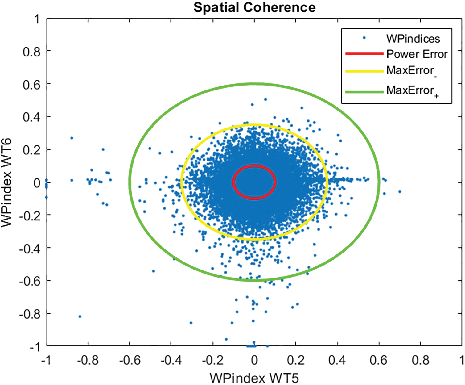
Figure 21: WT6 vs. WT5 Wind-Power Indices spatial coherence
In this case, according to Fig. 21, most of the points fall within the error margins, where both wind turbines operate correctly. The few points outside these margins could be due to transient. Furthermore, a very symmetrical point cloud is observed, meaning that both generators operate very similarly.
Fig. 22 shows a comparison of two turbines of type Adwen, WT11 and WT12, over a month. In this case, a diagonal of points can be seen that fall outside the error margins.
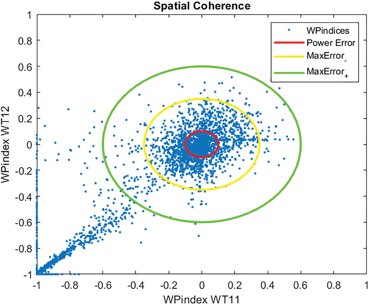
Figure 22: WT12 vs. WT11 Wind-Power Indices spatial coherence
This means that both wind turbines are generating less power than they should. But in this case, this degradation is symmetrical with respect to the main diagonal, so it can be deduced that it is not a failure of one of the wind turbines, but rather it can be assumed that it is a general failure of this type of turbines of the farm. But it can also be observed that WT11 suffers more power stops than WT12.
6.4 Spatiotemporal Coherence Analysis
Normalization of the signals and the wind power index also allows for the simultaneous analysis of both temporal and spatial coherence. In addition, normalization allows for the comparison of wind turbine performance with the average for the entire wind farm. The wind farm index can be defined as an average in Eq. (22), excluding wind turbines in a technical shutdown from this calculation.
By plotting the temporal evolution of the index for all wind turbines on a single graph, even if they are of different types or have undergone modifications during their useful life, their correlation in both domains can be observed. Fig. 23 shows a comparison of the temporal behavior of filtered indices of all the wind turbines (colors) and the farm average (black line).
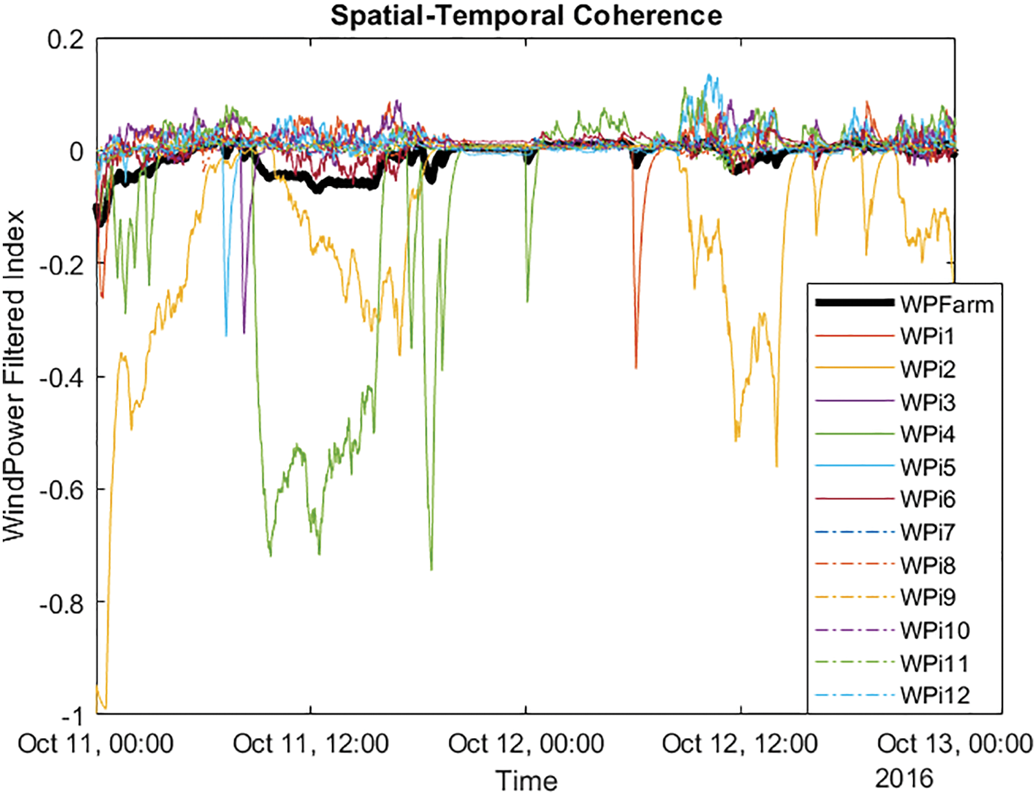
Figure 23: Wind Farm spatiotemporal coherence
From the analysis and observation of Fig. 23 it can be concluded that:
• All wind turbines, except WT2 and WT4, are behaving normally, exhibiting only small power anomalies for brief intervals due to short shutdowns.
• Wind turbine WT2 experienced multiple power anomalies over those days. Its signals were analyzed, revealing that it does not accurately measure the wind speed. As a result, the control system is in safe mode, not adjusting the blade pitch, causing performance degradation with partial drops in the index.
• Wind turbine WT4 also exhibits multiple power anomalies over significant time intervals. However, upon analysis of its wind and power signals, they appear to be correct. In the following days, this wind turbine underwent inspection and repair.
• Wind turbine WT5 shows a small spike regarding wind anomaly around 12:00 on day 12 of October.
• Due to the power drop at wind turbines WT2 and WT4, the farm produced 5% less than optimal power for most of day 11 and for a brief period on day 12 October.
This study presents a methodological contribution to anomaly detection in wind energy by focusing on data processing rather than specific application techniques. Normalizing turbine behavior variables proved to greatly facilitate the detection and interpretation of anomalies, enabling a clearer distinction between measurement errors and operational issues affecting power generation. The introduction of a simple quadratic power curve model, coupled with a Wind Power Index (WPi), has demonstrated its effectiveness in separating normal behavior from potential failures. Integrating a Support Vector Machine (SVM) into this framework improved the classification of subtle anomalies, especially in borderline cases with transient disturbances or measurement noise.
A key advantage of the proposed normalization approach is its ability to unify anomaly detection across turbines from different manufacturers. The linear WPi index, combined with normalized data, supports coherent temporal and spatial analysis, making anomaly identification more direct and interpretable. This framework can be adapted for real-time monitoring and detection, offering scalability across heterogeneous turbine models and diverse environmental conditions.
This study has certain limitations. The methodology was tested on two commercial wind turbine models from a single data set, which may restrict its generalizability without further validation on different wind farm installations. Direct quantitative comparison with other approaches is challenging due to the absence of publicly available data sets with similar operational constraints. Future work should focus on applying the method to broader and more varied data, integrating additional sensor measurements, and exploring its influence on advanced classification techniques. These steps would strengthen its robustness, adaptability, and applicability in both onshore and offshore wind energy contexts.
Acknowledgement: Not applicable.
Funding Statement: This work has been partially supported by the Spanish Ministry of Science and Innovation under the MCI/AEI/FEDER project number PID2021-123543OBC21.
Author Contributions: The authors confirm contribution to the paper as follows: conceptualization, Bassel Weiss and Matilde Santos; methodology, Bassel Weiss and Segundo Esteban; software, Bassel Weiss; validation, Bassel Weiss and Segundo Esteban; resources, Bassel Weiss and Matilde Santos; writing—original draft preparation, Bassel Weiss; writing—review and editing, Segundo Esteban and Matilde Santos; funding acquisition, Matilde Santos. All authors reviewed the results and approved the final version of the manuscript.
Availability of Data and Materials: The data supporting the findings of this study are accessible through RAVE (Research at Alpha Ventus), German Federal Ministry of Climate Action, coordinated by Fraunhofer IWES (https://rave-offshore.de/en/data.html, accessed on 8 August 2025).
Ethics Approval: Not applicable.
Conflicts of Interest: The authors declare no conflicts of interest to report regarding the present study.
Abbreviations
| ANNs | Artificial Neural Networks |
| BiGRU | Bidirectional Gated Recurrent Unit |
| BiLSTM | Bidirectional Long Short-Term Memory |
| CNN | Convolutional Neural Network |
| Con | Controlled |
| DBSCAN | Density-Based Spatial Clustering of Applications with Noise |
| DSTDS | Detectable Spatial and Temporal Dependence Structure |
| EPn | Normalized Electric Power |
| Fino1 | from German: Research Platform in the North and Baltic seas 1 |
| GCN | Graph Convolutional Network |
| GRU | Gated Recurrent Unit |
| iForest | Isolation Forest |
| k-NN | k-Nearest Neighbors |
| LSTM | Long Short-Term Memory |
| MANFIS | Multiple Adaptive Neuro-Fuzzy Inference System |
| MAX | Maximum |
| Min | Minimum |
| NLC-TCN | Non-Linear Controller-Temporal Convolutional Network |
| Oct | October |
| OWEC | Offshore Wind Energy Converter |
| OWT | Offshore Wind Turbine |
| qLPV | Quasi-Linear Parameter-Varying |
| RAVE | Research at Alpha Ventus |
| RBF | Radial Basis Function |
| RMSE | Root Mean Square Error |
| rpm | Revolutions per minute |
| SCADA | Supervisory Control and Data Acquisition |
| SVM | Support Vector Machine |
| TCN | Temporal Convolutional Network |
| WPi | Wind to Power Index |
| WSn | Normalized Wind Speed |
| WT | Wind Turbine |
References
1. Sacie M, Santos M, López R, Pandit R. Use of state-of-art machine learning technologies for forecasting offshore wind speed, wave and misalignment to improve wind turbine performance. J Mar Sci Eng. 2022;10(7):938. doi:10.3390/jmse10070938. [Google Scholar] [CrossRef]
2. Wang Y, Liu H, Li Q, Wang X, Zhou Z, Xu H, et al. Overview of condition monitoring technology for variable-speed offshore wind turbines. Energies. 2025;18(5):1026. doi:10.3390/en18051026. [Google Scholar] [CrossRef]
3. RAVE. Research at Alpha Ventus. RAVE-offshore.de. 2025. [cited 2025 May 1]. Available from: https://rave-offshore.de/en/start.html. [Google Scholar]
4. Masoumi M. Machine learning solutions for offshore wind farms: a review of applications and impacts. J Mar Sci Eng. 2023;11(10):1855. doi:10.3390/jmse11101855. [Google Scholar] [CrossRef]
5. Lind PG, Vera-Tudela L, Wächter M, Kühn M, Peinke J. Normal behaviour models for wind turbine vibrations: comparison of neural networks and a stochastic approach. Energies. 2017;10(12):1944. doi:10.3390/en10121944. [Google Scholar] [CrossRef]
6. Pandit R, Astolfi D, Hong J, Infield D, Santos M. SCADA data for wind turbine data-driven condition/performance monitoring: a review on state-of-art, challenges and future trends. Wind Eng. 2023;47(2):422–41. doi:10.1177/0309524X221124031. [Google Scholar] [CrossRef]
7. Vásquez-Rodríguez G, Maldonado-Correa J. Anomaly-based fault detection in wind turbines using unsupervised learning: a comparative study. IOP Conf Ser Earth Environ Sci. 2024;1370(1):012005. doi:10.1088/1755-1315/1370/1/012005. [Google Scholar] [CrossRef]
8. Kong K, Dyer K, Payne C, Hamerton I, Weaver PM. Progress and trends in damage detection methods, maintenance, and data-driven monitoring of wind turbine blades—a review. Renew Energy Focus. 2023;44:390–412. doi:10.1016/j.ref.2022.08.005. [Google Scholar] [CrossRef]
9. Kaewniam P, Cao M, Alkayem NF, Li D, Manoach E. Recent advances in damage detection of wind turbine blades: a state-of-the-art review. Renew Sustain Energy Rev. 2022;167(9):112723. doi:10.1016/j.rser.2022.112723. [Google Scholar] [CrossRef]
10. Bilendo F, Badihi H, Lu N, Cambron P, Jiang B. A normal behavior model based on power curve and stacked regressions for condition monitoring of wind turbines. IEEE Trans Instrum Meas. 2022;71:1–13. doi:10.1109/TIM.2022.3196116. [Google Scholar] [CrossRef]
11. Morrison R, Liu X, Lin Z. Anomaly detection in wind turbine SCADA data for power curve cleaning. Renew Energy. 2022;184:473–86. doi:10.1016/j.renene.2021.11.118. [Google Scholar] [CrossRef]
12. Martí-Puig P, Hernández JÁ., Solé-Casals J, Serra-Serra M. Enhancing reliability in wind turbine power curve estimation. Appl Sci. 2024;14(6):2479. doi:10.3390/app14062479. [Google Scholar] [CrossRef]
13. Zhang S, Robinson E, Basu M. Wind turbine condition monitoring based on three fitted performance curves. Wind Energy. 2024;27(5):429–46. doi:10.1002/we.2859. [Google Scholar] [CrossRef]
14. Astolfi D, Castellani F, Lombardi A, Terzi L. Multivariate SCADA data analysis methods for real-world wind turbine power curve monitoring. Energies. 2021;14(4):1105. doi:10.3390/en14041105. [Google Scholar] [CrossRef]
15. Bilendo F, Meyer A, Badihi H, Lu N, Cambron P, Jiang B, et al. Applications and modeling techniques of wind turbine power curve for wind farms—a review. Energies. 2022;16(1):180. doi:10.3390/en16010180. [Google Scholar] [CrossRef]
16. Paik C, Chung Y, Kim YJ. Power curve modeling of wind turbines through clustering-based outlier elimination. Appl Syst Innov. 2023;6(2):41. doi:10.3390/asi6020041. [Google Scholar] [CrossRef]
17. Chen W, Cheng L, Chang Z, Wen B, Li P. Wind turbine blade icing detection using a novel bidirectional gated recurrent unit with temporal pattern attention and improved coot optimization algorithm. Meas Sci Technol. 2022;34(1):014004. doi:10.1088/1361-6501/ac8db1. [Google Scholar] [CrossRef]
18. Wen W, Liu Y, Sun R, Liu Y. Research on anomaly detection of wind farm SCADA wind speed data. Energies. 2022;15(16):5869. doi:10.3390/en15165869. [Google Scholar] [CrossRef]
19. Xiang L, Yang X, Hu A, Su H, Wang P. Condition monitoring and anomaly detection of wind turbine based on cascaded and bidirectional deep learning networks. Appl Energy. 2022;305(15):117925. doi:10.1016/j.apenergy.2021.117925. [Google Scholar] [CrossRef]
20. Mehrjoo M, Jozani MJ, Pawlak M. Toward hybrid approaches for wind turbine power curve modeling with balanced loss functions and local weighting schemes. Energy. 2021;218(1):119478. doi:10.1016/j.energy.2020.119478. [Google Scholar] [CrossRef]
21. Chen N, Shao C, Wang G, Wang Q, Zhao Z, Liu X. Anomaly detection of wind turbine based on norm-linear-ConvNeXt-TCN. Meas Sci Technol. 2024;35(7):076107. doi:10.1088/1361-6501/ad366a. [Google Scholar] [CrossRef]
22. Miao Q, Wang D, Xia Z, Xu C, Zhan J, Wu C. Exploring spatio-temporal dynamics for enhanced wind turbine condition monitoring. Mech Syst Signal Process. 2025;223(6):111841. doi:10.1016/j.ymssp.2024.111841. [Google Scholar] [CrossRef]
23. Li Y, Shen X. Anomaly detection and classification method for wind speed data of wind turbines using spatiotemporal dependency structure. IEEE Trans Sustain Energy. 2023;14(4):2417–31. doi:10.1109/TSTE.2023.3270865. [Google Scholar] [CrossRef]
24. Cascianelli S, Astolfi D, Castellani F, Cucchiara R, Fravolini ML. Wind turbine power curve monitoring based on environmental and operational data. IEEE Trans Ind Inform. 2021;18(8):5209–18. doi:10.1109/TII.2021.3128205. [Google Scholar] [CrossRef]
25. Qian X, Sun T, Zhang Y, Wang B, Gendeel MAA. Wind turbine fault detection based on spatial-temporal feature and neighbor operation state. Renew Energy. 2023;219(2):119419. doi:10.1016/j.renene.2023.119419. [Google Scholar] [CrossRef]
26. Barnabei VF, Ancora TCM, Delibra G, Corsini A, Rispoli F. Semi-supervised deep learning framework for predictive maintenance in offshore wind turbines. Int J Turbomach Propuls Power. 2025;10(3):14. doi:10.3390/ijtpp10030014. [Google Scholar] [CrossRef]
27. Dai S, Han S, Bai X, Kang Z, Liu Y. A multivariate spatiotemporal feature fusion network for wind turbine gearbox condition monitoring. Energies. 2025;18(5):1273. doi:10.3390/en18051273. [Google Scholar] [CrossRef]
28. Li Y-F, Hu Z-A, Gao J-W, Zhang Y-S, Li P-F, Du H-Z. Efficient anomaly detection method for offshore wind turbines. J Electron Sci Technol. 2025;22(4):100285. doi:10.1016/j.jnlest.2024.10028. [Google Scholar] [CrossRef]
29. Miele ES, Bonacina F, Corsini A. Deep anomaly detection in horizontal axis wind turbines using graph convolutional autoencoders for multivariate time series. Energy AI. 2022;8(4):100145. doi:10.1016/j.egyai.2022.100145. [Google Scholar] [CrossRef]
30. Kong Z, Tang B, Deng L, Liu W, Han Y. Condition monitoring of wind turbines based on spatio-temporal fusion of SCADA data by convolutional neural networks and gated recurrent units. Renew Energy. 2020;146(C):760–8. doi:10.1016/j.renene.2019.07.033. [Google Scholar] [CrossRef]
31. Pérez-Pérez EJ, Puig V, López-Estrada FR, Valencia-Palomo G, Santos-Ruiz I, Osorio-Gordillo G. Robust fault diagnosis of wind turbines based on MANFIS and zonotopic observers. Expert Syst Appl. 2024;235(6):121095. doi:10.1016/j.eswa.2023.121095. [Google Scholar] [CrossRef]
32. Pérez-Pérez EJ, Puig V, López-Estrada FR, Valencia-Palomo G. Fault detection and isolation in wind turbines based on neuro-fuzzy qLPV zonotopic observers. Mech Syst Signal Process. 2023;191(7503):110025. doi:10.1016/j.ymssp.2023.110183. [Google Scholar] [CrossRef]
33. Pettas V, Kretschmer M, Clifton A, Cheng PW. On the effects of inter-farm interactions at the offshore wind farm Alpha Ventus. Wind Energy Sci. 2021;6(6):1455–72. doi:10.5194/wes-6-1455-2021. [Google Scholar] [CrossRef]
34. Durstewitz M, Lange B. Sea-wind-power: research at the first German offshore wind farm Alpha Ventus. Berlin/Heidelberg, Germany: Springer-Verlag GmbH; 2017. 252 p. doi:10.1007/978-3-662-53179-2. [Google Scholar] [CrossRef]
35. Nassif AB, Talib MA, Nasir Q, Dakalbab FM. Machine learning for anomaly detection: a systematic review. IEEE Access. 2021;9:78658–700. doi:10.1109/ACCESS.2021.3083060. [Google Scholar] [CrossRef]
Cite This Article
 Copyright © 2025 The Author(s). Published by Tech Science Press.
This work is licensed under a Creative Commons Attribution 4.0 International License , which permits unrestricted use, distribution, and reproduction in any medium, provided the original work is properly cited.
 Downloads
 Citation Tools