
 Submit a Paper
 Propose a Special lssue
 Open Access
ARTICLE

Dombi Power Aggregation-Based Decision Framework for Smart City Initiative Prioritization under t-Arbicular Fuzzy Environment
1 Institute of Numerical Sciences, Kohat University of Science and Technology, Kohat, 26000, Khyber Pakhtunkhwa, Pakistan
2 Department of Computing, Mathematics and Electronics, “1 Decembrie 1918” University of Alba Iulia, Alba Iulia, 510009, Romania
3 Faculty of Mathematics and Computer Science, Transilvania University of Brasov, Iuliu Maniu Street 50, Brasov, 500091, Romania
* Corresponding Author: Jawad Ali. Email:
(This article belongs to the Special Issue: Algorithms, Models, and Applications of Fuzzy Optimization and Decision Making)
Computer Modeling in Engineering & Sciences 2025, 145(1), 857-889. https://doi.org/10.32604/cmes.2025.064604
Received 19 February 2025; Accepted 29 July 2025; Issue published 30 October 2025
 View Full Text
 Download PDF
Abstract
With the rapid growth of urbanization, smart city development has become a strategic priority worldwide, requiring complex and uncertain decision-making processes. In this context, advanced decision-support tools are essential to evaluate and prioritize competing initiatives effectively. To support effective prioritization of smart city initiatives under uncertainty, this study introduces a robust decision-making framework based on the t-arbicular fuzzy (t-AF) set—a recent extension of the t-spherical fuzzy set that incorporates an additional parameter, the radius , to enhance the representation of uncertainty. Dombi-based operational laws are formulated within this context, leading to the development of four power aggregation operators that integrate a support degree to reflect inter-attribute relationships. The structural and theoretical foundations of the operators are rigorously demonstrated. Further, the proposed operators are embedded into an extended weighted aggregated sum product assessment (WASPAS) method to create a comprehensive multi-criteria decision-making model. The practical utility of the proposed approach is demonstrated through a case study involving the evaluation of seven smart city initiatives against eight critical criteria. Comparative analysis against established models reveals that the proposed approach offers superior ranking consistency, enhanced discrimination power among alternatives, and improved handling of uncertainty—ultimately supporting more reliable and interpretable decision-making outcomes.Keywords
Multi-criteria decision-making (MCDM) refers to the systematic evaluation and selection of the most suitable alternative from a set of options, each assessed against multiple, and often conflicting, criteria, constraints, and objectives [1–4]. This process is integral to a wide range of domains—from routine personal choices to complex strategic decisions in business and public policy—where it facilitates rational analysis and prioritization. As real-world decision problems frequently involve ambiguous or incomplete information, effective MCDM strategies must account for such uncertainty. To address this, Zadeh [5] introduced the fuzzy set (FS) theory, which allows partial membership values rather than strict binary categorization. Subsequently, Atanassov [6] enhanced this framework by proposing intuitionistic FS (IFS), incorporating degrees of non-membership alongside membership. Later, Yager and Abbasov [7] advanced the theory further through the introduction of Pythagorean FS (PyFS), offering an even more nuanced mechanism for uncertainty representation.
While IFS and PyFS have proven to be effective tools within the broader FS theory, they share a significant shortcoming: their frameworks do not fully accommodate ambiguous or indeterminate opinions that cannot be classified strictly in terms of membership or non-membership. To bridge this conceptual gap, Cuong and Kreinovich [8] proposed the Picture FS (PFS), a more expressive model that permits the representation of human judgments across four distinct dimensions—positive, negative, neutral (abstention), and refusal. This allows decision-makers to express more nuanced evaluations in complex environments. However, like IFS, the PFS model imposes a constraint that the sum of the three primary degrees must not exceed one, limiting its capacity to represent broader uncertainty. To overcome this structural limitation, Mahmood et al. [9] introduced the spherical FS (SFS), a generalization of PFS that defines its membership components on the surface of a unit sphere, thus relaxing the additive constraint and offering a richer modeling framework. Since then, SFS theory has gained traction in decision sciences. Al-Shamiri et al. [10] extended the SFS framework to spherical fuzzy bipolar soft expert sets by introducing certain set-theoretic operations and properties for the proposed model, and addressed several important related problems. Sarwar et al. [11] introduced a quantum spherical fuzzy approach to the technique for order preference by similarity to ideal solution method, incorporating elements from quantum mechanics and fuzzy logic. Further advancements include Ali and Garg’s [12] formulation of a norm-based distance metric specific to SFS, and Akram et al.’s [13] exploration of outranking techniques under the same environment. Recently, Ali [14] proposed a symmetry-based ranking approach tailored to sustainable supplier evaluation using SFS. Building upon these developments, Ashraf et al. [15,16] introduced an extended version of the SFS model known as the disc SFS (DSFS), which incorporates an additional radius parameter. This enhancement allows the model to capture variable levels of fuzziness, providing a more flexible and realistic depiction of uncertainty in practical decision-making contexts. Unlike traditional SFS, where the degree values are constrained to lie on the unit sphere, the DSFS introduces a disc-like geometry that adjusts the scale of uncertainty representation. This additional parameter facilitates a more granular differentiation among alternatives and enhances the accuracy of aggregation operations—capabilities that conventional FS models often lack. However, DSFS imposes a rigid constraint that the sum of the squares of the three membership-related components must not exceed unity, i.e.,
Aggregation operators (AOs) serve as essential tools in real-world decision-making by enabling the synthesis and prioritization of fuzzy information. Over time, researchers have proposed numerous AOs tailored to various fuzzy frameworks. For example, Jana et al. [18] formulated Dombi-based operators within the context of Pythagorean fuzzy sets. Senapati et al. [19] advanced the field by introducing Aczel-Alsina operators for interval-valued intuitionistic fuzzy settings, highlighting their practical relevance in decision analysis. Qiyas et al. [20] explored trigonometric sine-based operators for spherical fuzzy sets to address decision-making challenges, while in a separate study, Qiyas et al. [21] presented Hamacher-type operators for spherical uncertain linguistic environments, emphasizing their applicability in group decision scenarios to unify divergent expert opinions. Similarly, Abdullah et al. [22] conducted an in-depth assessment of decision support systems grounded in 2-tuple spherical fuzzy linguistic aggregation methods.
The Dombi AO, originally formulated by Dombi in 1982 [23], is characterized by its parameter-dependent adaptability, enabling it to function in either a conjunctive or disjunctive mode. This intrinsic flexibility has led to its extensive adaptation within a range of fuzzy set extensions. For instance, Chen and Ye [24] introduced weighted Dombi operators under single-valued neutrosophic sets, establishing a foundational approach for subsequent enhancements. Expanding on this, Liu et al. [25] incorporated the Dombi Bonferroni mean into IFS theory and applied it to MCDM. Similarly, Shi and Ye [26] explored the application of Dombi operators in neutrosophic cubic environments to address MCDM scenarios. More recent advancements include the work of Seikh and Mandal [27], who developed interval-valued Fermatean fuzzy Dombi weighted operators and extended them to interval-valued spherical fuzzy domains, with practical implementation in areas such as plastic waste management [28]. Furthermore, Jana et al. [18] adapted the Dombi operator to picture FSs, thereby broadening its operational landscape. In a recent development, Seikh and Mandal [29] introduced a new class of Dombi averaging and geometric AOs for IFS, applying them to MCDM problems. Despite extensive research on Dombi aggregation operations across various FS extensions, disc spherical fuzzy (DSF) operations have not yet been defined in terms of Dombi operations. Consequently, existing DSF AOs primarily rely on the algebraic product and sum of DSFs, making them less generalized. Moreover, conventional operators often overlook the mutual dependencies among the input values being aggregated, which significantly undermines their suitability for handling intricate decision-making problems. To overcome this shortcoming, and guided by the foundational principles of power aggregation [30–32], it becomes essential to construct a new class of aggregation operators under the DSF environment, wherein the weights are adaptively determined based on the characteristics of the input data. Incorporating Dombi-based operations into this scheme enhances the mutual reinforcement among the aggregated inputs, yielding more coherent and context-sensitive results. Additionally, these advancements call for the application of the weighted aggregated sum product assessment (WASPAS) method in conjunction with the newly proposed operators. A significant benefit of this integrated strategy lies in its capacity to reduce the impact of outliers and unfavorable inputs by leveraging power-based weights within a flexible, hybrid MCDM framework. This methodology combines the advantages of the weighted sum model (WSM) and the weighted product model (WPM), enabling a more stable and discriminative ranking of alternatives. WASPAS produces final scores by synthesizing the outcomes from both models, with its operational mode governed by a threshold parameter. Depending on the selected value, the method can emulate either WSM or WPM behavior, thus drawing on the respective merits of both approaches.
Despite notable progress in fuzzy MCDM, several methodological and practical limitations persist, which serve as the motivation for this study:
i. Lack of Dombi AOs in DSF environments: Although Dombi AOs are recognized for their parametric flexibility and generalization capabilities [23], they have not yet been incorporated into DSF frameworks. Existing DSF aggregation models primarily rely on conventional algebraic operations, limiting their adaptability in handling complex uncertainties.
ii. Static weighting in DSF aggregation: Current DSF-based AOs utilize fixed weighting schemes, failing to reflect the contextual influence of input data. Inspired by power aggregation mechanisms [30–32], there exists a need to develop DSF-based AOs that dynamically adjust weights in response to varying input arguments, thereby better representing expert judgment and preferences.
iii. Lack of hybrid aggregation strategies: Many DSF-based MCDM approaches are restricted to either WSM or WPM, which can limit their robustness in multifactorial decision environments. The hybrid WASPAS method, which balances additive and multiplicative reasoning, has not been adapted to the DSF context.
iv. Underexplored application in smart city prioritization: To the best of the authors’ knowledge, no prior study has applied DSF-based MCDM frameworks—particularly those involving Dombi operators and hybrid power aggregation—to the domain of smart city initiative prioritization. Given the inherent complexity, uncertainty, and interdependence of smart city components, this application provides an ideal platform to validate the practical value and broader applicability of the proposed model.
Based on the above gaps, this research presents the following contributions:
i. A novel class of DSF AOs based on Dombi functions, enhancing flexibility and generalization in fuzzy environments.
ii. Integration of power aggregation into DSF AOs, allowing context-sensitive weight adjustment that better reflects the influence of input data.
iii. Extension of the WASPAS methodology to the DSF framework using Dombi-based AOs, resulting in improved ranking stability and decision accuracy.
iv. Implementation of the proposed model in a real-world case study on smart city initiative prioritization—an application area not previously addressed in the DSF-MCDM literature—to demonstrate its practical relevance and effectiveness.
The structure of this article is as follows: Section 2 reviews the foundational concepts necessary to comprehend the proposed framework. In Section 3, the formulation and properties of Dombi operations under the DSF environment are explored in detail. Section 4 introduces a set of aggregation operators based on these operations. Section 5 describes the procedural steps of the WASPAS technique, which is then employed in a practical case study in Section 6. Section 7 provides a comparative evaluation to assess the effectiveness of the proposed model. Concluding remarks are offered in Section 8.
In this article, the set
This section reviews the definitions of DTN, DTCN, and power operators, as well as t-SFS and t-AFS, along with their corresponding theoretical concepts.
Definition 1. [23] For
Definition 2. [30] Given a sequence of non-negative real numbers
Here,
i)
Moreover, the support measure is defined as
Definition 3. [31] Consider a sequence of non-negative real numbers
The variables are specified in the same manner as in Definition 2.
Definition 4. [9] A t-SFS
where
Definition 5. [9,33] Let
1.
2.
3.
4.
Definition 6. [34] Consider
The greater the score function value, the higher the ranking of the corresponding t-SFN.
Definition 7. [17] A t-AFS on
where
The expression
Definition 8. [17] Let
1.
2.
3.
4.
5.
Definition 9. [17] Let
where
In this section, we establish the Dombi operational laws tailored for t-AFNs, laying the groundwork for subsequent aggregation mechanisms.
Definition 10. Consider two t-AFNs,
1.
2.
3.
4.
Building on the t-AFN operations outlined in Section 3, we introduce a set of Dombi power operators and examine their resulting properties.
4.1 t-AF Dombi Power Average Operator
In the present part, we establish the theoretical foundation of the t-AFDPA operator and explore its characteristics.
Definition 11. For a given set of t-AFNs
Here,
Theorem 1. Given a set of t-AFNs
Proof. This can be proven using mathematical induction as follows:
For
Assume that Eq. (12) holds for
Now, to prove it for
Therefore, Eq. (12) holds for all
Theorem 2. For a given set of t-AFNs
Proof. Since
Theorem 3. For any two sets of t-AFNs,
Proof. As
Furthermore, given that
Additionally, since
Hence, we obtain
Theorem 4. For any sequence of t-AFNs given by
Proof. Given that
Therefore,
4.2 t-AF Dombi Power Weighted Average Operator
Definition 12. For a given set of t-AFNs
here,
Theorem 5. For any set of t-AFNs given by
Theorem 6. For any collection of t-AFNs represented as
Theorem 7. For any two sets of t-AFNs, denoted as
Theorem 8. For any set of t-AFNs given by
4.3 t-AF Dombi Power Geometric Operator
In the present section, we establish the theoretical foundation of the t-AFDPG operator and analyze its properties.
Definition 13. For a given set of t-AFNs
here,
Theorem 9. For any collection of t-AFNs represented as
Proof. This can be proven using mathematical induction as follows:
For the base case
Assume that Eq. (22) holds for
Now, to prove it for
Therefore, Eq. (22) holds for all
Theorem 10. For a given set of t-AFNs
Proof. Given that
Theorem 11. Consider two sets of t-AFNs, denoted as
Proof. Given that
Furthermore, since
Moreover, since
Theorem 12. For any set of t-AFNs represented as
and
then the following holds.
Proof. Given that
We derive the following inequalities.
Therefore,
4.4 t-AF Dombi Power Weighted Geometric Operator
Definition 14. Given an array of t-AFNs defined as
here,
Theorem 13. Given an array of t-AFNs
Theorem 14. Consider an array of t-AFNs
Theorem 15. Given two arrays of t-AFNs,
Theorem 16. Consider an array of t-AFNs
This section presents a WASPAS-based method that incorporates the developed power AOs. Let
Decision experts assess each criteria
The following steps describe the procedure of the proposed t-AF-WASPAS method:
Step 1: Normalize the decision matrix
Step 2: Calculate the support value for each criteria
where
Step 3: Determine the total support for
Then, compute the power weight corresponding to
here,
Step 4: Apply the t-AFDPWA operator to calculate the WSM
Step 5: Use the t-AFDPWG operator to calculate the WPM
Step 6: Using Eq. (37), combine the WSM and WPM values to obtain the aggregated preference measure
here,
Step 7: Calculate the score of each aggregated preference measure
The pseudocode representation of the proposed WASPAS approach is provided in Algorithm 1.

The stepwise procedure of the proposed methodology is depicted in Fig. 1.

Figure 1: Flowchart of the proposed WASPAS method
6 Case Study: Smart City Initiative Prioritization
In the following, we explore the smart city initiative prioritization problem, and implement the proposed algorithm to showcase its practical applicability and effectiveness.
The rapid expansion of urban populations worldwide has intensified the challenges faced by cities in managing infrastructure, resources, sustainability, and overall quality of life. In response to these growing concerns, the concept of smart cities has gained significant attention, promoting the integration of digital technologies, data-driven systems, and automation to create more livable, efficient, and sustainable urban environments.
However, the successful development of smart cities demands careful prioritization across diverse domains such as energy, healthcare, governance, transportation, and public safety. Given the limitations in financial resources, technological maturity, and public readiness, it is impractical to implement all smart initiatives simultaneously. Consequently, there is a pressing need for a structured approach to prioritize projects based on their potential impact and feasibility.
Due to the multi-dimensional and often conflicting nature of the factors involved, this decision-making process is complex. Therefore, the application of MCDM problems provides a systematic and rational mechanism to evaluate and rank different initiatives by considering both qualitative and quantitative aspects.
In this study, an MCDM-based framework is proposed to prioritize a selection of seven smart city initiatives evaluated against eight critical criteria, aiming to assist urban planners and decision-makers in adopting strategies that are both effective and sustainable.
Evaluation Criteria: The assessment of smart city initiatives is conducted based on eight carefully selected criteria, as presented in Table 1.

Alternatives: The evaluation considers seven selected smart city initiatives, summarized in Table 2.

A panel of experts evaluates seven smart city initiatives
In the present section, we employ the proposed WASPAS approach to the data provided in Matrix
Step 1: Since the criteria
Step 2: Based on Eq. (32), the support values are calculated as given below:
Step 3: Using Eqs. (33) and (34), the power weights are calculated and presented in the following matrix.
Step 4: According to Eq. (35), the weighted sum measures
Step 5: Using Eq. (36), the weighted product measures
Step 6: Applying Eq. (37) with
Step 7: The scores of the aggregated preference measures are calculated as follows:
Consequently, the ranking of the projects is:
6.3 Theoretical and Policy Implications
Theoretical Implications: This study offers several significant contributions to the field of fuzzy MCDM. Firstly, it enhances the modeling of uncertainty through the use of t-AF sets, incorporating a radius component for a richer and more flexible representation. Secondly, the development of Dombi-based aggregation operators provides an improved mechanism for addressing interdependencies among criteria, a frequently encountered but often underexplored issue. Furthermore, the integration of the WASPAS method within the disc spherical fuzzy environment introduces a robust and efficient mechanism for ranking alternatives, effectively balancing both additive and multiplicative assessment strategies. Collectively, these innovations advance the methodological foundation for researchers tackling high-dimensional and uncertainty-laden decision problems.
Policy Implications: From a practical standpoint, the proposed t-AF-WASPAS method can assist policymakers and planners in making more informed decisions about renewable energy projects. It offers a clear, adaptable structure for evaluating projects based on technical, environmental, and social factors. Importantly, it also accounts for risks related to policy or market changes—an essential feature in today’s evolving energy landscape. By aligning with broader sustainability goals and national development targets, this approach supports strategic, long-term planning at various scales—from local initiatives to national programs.
This section conducts a detailed sensitivity analysis to evaluate the impact of the parameter
As shown in Table 3, the ranking scores and corresponding preference orderings remain remarkably stable across different values of

Minor shifts are observed in the middle-ranked alternatives (e.g.,
Next, we conduct the sensitivity with respect to the parameter

From the results, it is observed that when
From
This section presents a comprehensive evaluation of the proposed methodology by comparing its outcomes with various alternative methods previously reported in the literature [16,35–40]. The outcomes derived are presented in Table 5.
(1). From Table 5, it is evident that the operators CSFSWWA and CSFSWWG proposed by Ashraf et al. [16] identify
(2). From Table 5, it can be observed that the DSF-AAWA and DSF-AAWG operators proposed by Ahmad et al. [35] identify
However, a notable limitation in both [35] and [36] lies in their use of the score function defined as
(3). In comparison with the approaches proposed by Ashraf et al. [37] and Revathy et al. [38], the radius and neutral components were omitted, respectively, from the dataset in matrix
(4). From Table 5, it is evident that

Moreover, Table 6 presents a detailed comparative overview of the proposed approach and the existing methods, highlighting the key characteristics, advantages, and limitations of each.

While the proposed WASPAS-based model offers improved decision-making performance in uncertain environments, several limitations should be acknowledged. (i) The current framework is designed for MCDM problems and may not extend directly to MCGDM settings without further adaptation. (ii) Its reliance on fuzzy data—particularly membership, non-membership, neutrality, and the radius parameter—limits its applicability in crisp decision environments where such inputs are unavailable. (iii) The method treats input criteria as independent and lacks the ability to model interrelationships among them, unlike techniques that use Maclaurin symmetric means or other dependency-aware aggregators. (iv) It also does not support partitioned input structures, which restricts its suitability for hierarchical or thematically grouped criteria. (v) The model’s effectiveness depends on predefined weight values, making it sensitive to subjective or imprecise weight assignments. In contrast, hybrid or data-driven weighting strategies offer greater flexibility. (vi) Lastly, although the method performs well for moderate problem sizes, handling very large decision matrices may still pose computational challenges compared to more scalable approaches like CRADIS.
To overcome the aforementioned limitations, future developments of the framework could focus on incorporating inter-attribute dependency modeling, introducing hybrid weighting mechanisms, enhancing computational scalability for high-dimensional decision problems, and conducting broader real-world validations to improve its generalizability and practical relevance.
In order to statistically validate the robustness of the proposed method in comparison with the existing approach, we apply the Spearman correlation test on the ranking results presented in Table 6. The obtained correlation coefficients between different ranking vectors are graphically illustrated in the heatmap shown in Fig. 2.
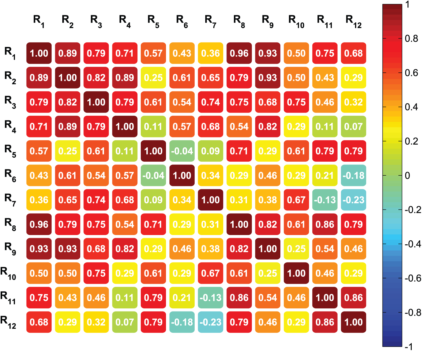
Figure 2: Spearman correlation between rankings
The results, visualized in the heatmap in Fig. 2, reveal that the proposed method (
This study introduced a novel decision-making methodology based on the Dombi operational framework under the t-AF environment. A family of four new aggregation operators—t-AFDPA, t-AFDPWA, t-AFDPG, and t-AFDPWG—was developed by incorporating power weights to effectively capture interrelationships among input arguments while minimizing the influence of extreme values. These operators demonstrate an enhanced capacity to handle complex decision information by integrating support degrees among inputs. A mathematical analysis confirmed the desirable properties of the proposed operators, ensuring their consistency, monotonicity, and idempotency. To operationalize the framework, the WASPAS method was modified to accommodate t-AF data and employed in a realistic decision-making scenario related to smart city initiative prioritization. The results showcased the practicality and effectiveness of the approach, particularly in capturing the nuanced nature of uncertainty and vagueness present in complex environments. A detailed sensitivity analysis, as illustrated in Tables 5 and 6, revealed that the model exhibits strong robustness against variations in both critical parameters—
Future research could focus on extending the proposed t-AF-based aggregation framework to other advanced decision-making domains, particularly those involving machine learning-driven models, graph theory-based approaches and three-way decision models, where the presence of uncertainty and imprecision is a critical challenge. Additionally, the integration of this framework with hybrid MCDM techniques and confidence-level-based decision strategies could significantly enhance its flexibility and practical applicability in complex, multi-criteria environments.
Acknowledgement: Not applicable.
Funding Statement: The authors received no specific funding for this study.
Author Contributions: Conceptualization, Jawad Ali; methodology, Ioan-Lucian Popa; software, Jawad Ali; validation, Ioan-Lucian Popa; formal analysis, Jawad Ali; writing—original draft preparation, Jawad Ali and Ioan-Lucian Popa; writing—review and editing, Jawad Ali and Ioan-Lucian Popa. All authors reviewed the results and approved the final version of the manuscript.
Availability of Data and Materials: Our manuscript has no associated data.
Ethics Approval: Not applicable.
Conflicts of Interest: The authors declare no conflicts of interest to report regarding the present study.
Abbreviations
| MCDM | Multi-criteria decision-making |
| FS | Fuzzy set |
| IFS | Intuitionistic fuzzy set |
| PyFS | Pythagorean fuzzy set |
| PFS | Picture fuzzy set |
| SFS | Spherical fuzzy set |
| DSFS | Disc spherical fuzzy set |
| t-AFS | t-Arbicular fuzzy set |
| AOs | Aggregation operators |
| t-AFN | t-Arbicular fuzzy number |
| WASPAS | Weighted aggregated sum product assessment |
| PA | Power average |
| DTN | Dombi t-norm |
| DTCN | Dombi t-conorm |
| PG | Power geometric |
| SFN | Spherical fuzzy number |
| WPA | Weighted power average |
| WPG | Weighted power geometric |
| SFN | Spherical fuzzy number |
| DSFN | Disc spherical fuzzy number |
| WSM | Weighted sum measure |
| WPM | Weighted product measure |
| DSFDPA | Disc spherical fuzzy Dombi power average |
| MCGDM | Multi-criteria group decision-making |
| DSFDPWA | Disc spherical fuzzy Dombi power weighted geometric |
| DSFDPG | Disc spherical fuzzy Dombi power geometric |
| DSFDPWG | Disc spherical fuzzy Dombi power weighted average |
| DSFN | Disc spherical fuzzy number |
References
1. Ali Z. Fairly aggregation operators based on complex p, q-rung orthopair fuzzy sets and their application in decision-making problems. Spec Oper Res. 2025;2(1):113–31. doi:10.1007/s40314-021-01696-z. [Google Scholar] [CrossRef]
2. Ali J, Ali W, Alqahtani H, Syam MI. Enhanced EDAS methodology for multiple-criteria group decision analysis utilizing linguistic q-rung orthopair fuzzy hamacher aggregation operators. Complex Intell Syst. 2024;10(6):8403–32. doi:10.1007/s40747-024-01586-x. [Google Scholar] [CrossRef]
3. Li D, Wan G, Rong Y. An enhanced spherical cubic fuzzy waspas method and its application for the assessment of service quality of crowdsourcing logistics platform. Spec Decis Mak Appl. 2026;3(1):100–23. [Google Scholar]
4. Petchimuthu S, Mahendiran C, Premala T. Power and energy transformation: multi-criteria decision-making utilizing complex q-rung picture fuzzy generalized power prioritized Yager operators. Spec Oper Res. 2025;2(1):219–58. [Google Scholar]
5. Zadeh LA. Fuzzy sets. Inf Control. 1965;8(3):338–53. [Google Scholar]
6. Atanassov K. Intuitionistics fuzzy sets. Fuzzy Sets Syst. 1986;20(1):87–96. doi:10.1016/s0165-0114(86)80034-3. [Google Scholar] [CrossRef]
7. Yager RR, Abbasov AM. Pythagorean membership grades, complex numbers, and decision making. Int J Intell Syst. 2013;28(5):436–52. doi:10.1002/int.21584. [Google Scholar] [CrossRef]
8. Cuong BC, Kreinovich V. Picture fuzzy sets-a new concept for computational intelligence problems. In: 2013 Third World Congress on Information and Communication Technologies (WICT 2013); 2013 Dec 15–18; Hanoi, Vietnam: IEEE; 2013. p. 1–6. [Google Scholar]
9. Mahmood T, Ullah K, Khan Q, Jan N. An approach toward decision-making and medical diagnosis problems using the concept of spherical fuzzy sets. Neural Comput Appl. 2019;31(11):7041–53. doi:10.1007/s00521-018-3521-2. [Google Scholar] [CrossRef]
10. Al-Shamiri MMA, Ali G, Abidin MZU, Adeel A. Multi-attribute group decision-making method under spherical fuzzy bipolar soft expert framework with its application. Comput Model Eng Sci. 2023;137(2):1891–936. doi:10.32604/cmes.2023.027844. [Google Scholar] [CrossRef]
11. Sarwar MA, Gong Y, Alzakari SA, Alhussan AA. Quantum-driven spherical fuzzy model for best gate security systems. Comput Model Eng Sci. 2025;143(3):3523–55. doi:10.32604/cmes.2025.066356. [Google Scholar] [CrossRef]
12. Ali J, Garg H. On spherical fuzzy distance measure and TAOV method for decision-making problems with incomplete weight information. Eng Appl Artif Intell. 2023;119(7):105726. doi:10.1016/j.engappai.2022.105726. [Google Scholar] [CrossRef]
13. Akram M, Zahid K, Kahraman C. A PROMETHEE based outranking approach for the construction of Fangcang shelter hospital using spherical fuzzy sets. Artif Intell Med. 2023;135(10232):102456. doi:10.1016/j.artmed.2022.102456. [Google Scholar] [PubMed] [CrossRef]
14. Ali J. Spherical fuzzy symmetric point criterion-based approach using Aczel-Alsina prioritization: application to sustainable supplier selection. Granul Comput. 2024;9(2):33. doi:10.1007/s41066-024-00449-7. [Google Scholar] [CrossRef]
15. Ashraf S, Chohan MS, Ahmad S, Hameed MS, Khan F. Decision aid algorithm for kidney transplants under disc spherical fuzzy sets with distinctive radii information. IEEE Access. 2023;11:122029–44. doi:10.1109/access.2023.3327830. [Google Scholar] [CrossRef]
16. Ashraf S, Iqbal W, Ahmad S, Khan F. Circular spherical fuzzy sugeno weber aggregation operators: a novel uncertain approach for adaption a programming language for social media platform. IEEE Access. 2023;11:124920–41. doi:10.1109/access.2023.3329242. [Google Scholar] [CrossRef]
17. Ali J, Popa I-L. TODIM method with unknown weights under t-arbicular fuzzy environment for optimal gate security system selection. AIMS Math. 2025;10(6):13941–73. doi:10.3934/math.2025627. [Google Scholar] [CrossRef]
18. Jana C, Senapati T, Pal M, Yager RR. Picture fuzzy Dombi aggregation operators: application to MADM process. Appl Soft Comput. 2019;74(4):99–109. doi:10.1016/j.asoc.2018.10.021. [Google Scholar] [CrossRef]
19. Senapati T, Chen G, Mesiar R, Yager RR, Saha A. Novel Aczel-Alsina operations-based hesitant fuzzy aggregation operators and their applications in cyclone disaster assessment. Int J Gen Syst. 2022;51(5):511–46. doi:10.1080/03081079.2022.2036140. [Google Scholar] [CrossRef]
20. Qiyas M, Abdullah S, Khan S, Naeem M. Multi-attribute group decision making based on sine trigonometric spherical fuzzy aggregation operators. Granul Comput. 2022;7(1):141–62. doi:10.1007/s41066-021-00256-4. [Google Scholar] [PubMed] [CrossRef]
21. Qiyas M, Abdullah S, Naeem M. Spherical uncertain linguistic Hamacher aggregation operators and their application on achieving consistent opinion fusion in group decision making. Int J Intell Comput Cybern. 2021;14(4):550–79. doi:10.1108/ijicc-09-2020-0120. [Google Scholar] [CrossRef]
22. Abdullah S, Barukab O, Qiyas M, Arif M, Khan SA. Analysis of decision support system based on 2-tuple spherical fuzzy linguistic aggregation information. Appl Sci. 2019;10(1):276. doi:10.3390/app10010276. [Google Scholar] [CrossRef]
23. Dombi J. A general class of fuzzy operators, the Demorgan class of fuzzy operators and fuzziness measures induced by fuzzy operators. Fuzzy Sets Syst. 1982;8(2):149–63. doi:10.1016/0165-0114(82)90005-7. [Google Scholar] [CrossRef]
24. Chen J, Ye J. Some single-valued neutrosophic Dombi weighted aggregation operators for multiple attribute decision-making. Symmetry. 2017;9(6):82. doi:10.3390/sym9060082. [Google Scholar] [CrossRef]
25. Liu P, Liu J. Some q-rung orthopai fuzzy Bonferroni mean operators and their application to multi-attribute group decision making. Int J Intell Syst. 2018;33(2):315–47. doi:10.1002/int.21933. [Google Scholar] [CrossRef]
26. Shi L, Ye J. Dombi aggregation operators of neutrosophic cubic sets for multiple attribute decision-making. Algorithms. 2018;11(3):29. doi:10.3390/a11030029. [Google Scholar] [CrossRef]
27. Seikh MR, Mandal U. Interval-valued fermatean fuzzy Dombi aggregation operators and SWARA based PROMETHEE II method to bio-medical waste management. Expert Syst Appl. 2023;226(3514):120082. doi:10.1016/j.eswa.2023.120082. [Google Scholar] [CrossRef]
28. Mandal U, Seikh MR. Interval-valued spherical fuzzy MABAC method based on Dombi aggregation operators with unknown attribute weights to select plastic waste management process. Appl Soft Comput. 2023;145(2):110516. doi:10.1016/j.asoc.2023.110516. [Google Scholar] [CrossRef]
29. Seikh MR, Chatterjee P. Evaluation and selection of E-learning websites using intuitionistic fuzzy confidence level based Dombi aggregation operators with unknown weight information. Appl Soft Comput. 2024;163(1):111850. doi:10.1016/j.asoc.2024.111850. [Google Scholar] [CrossRef]
30. Yager RR. The power average operator. IEEE Trans Syst Man Cybern Part A Syst Humans. 2001;31(6):724–31. doi:10.1109/3468.983429. [Google Scholar] [CrossRef]
31. Xu Z, Yager RR. Power-geometric operators and their use in group decision making. IEEE Trans Fuzzy Syst. 2009;18(1):94–105. doi:10.1109/tfuzz.2009.2036907. [Google Scholar] [CrossRef]
32. Ali J. Multiple criteria decision-making based on linguistic spherical fuzzy copula extended power aggregation operators. Granul Comput. 2024;9(2):44. doi:10.1007/s41066-024-00464-8. [Google Scholar] [CrossRef]
33. Ashraf S, Abdullah S, Mahmood T, Ghani F, Mahmood T. Spherical fuzzy sets and their applications in multi-attribute decision making problems. J Intell Fuzzy Syst. 2019;36(3):2829–44. [Google Scholar]
34. Ju Y, Liang Y, Luo C, Dong P, Gonzalez EDS, Wang A. T-spherical fuzzy TODIM method for multi-criteria group decision-making problem with incomplete weight information. Soft Comput. 2021;25(4):2981–3001. doi:10.1007/s00500-020-05357-x. [Google Scholar] [CrossRef]
35. Ahmad QA, Ashraf S, Iqbal W, Qiang ML. Enhanced decision technique for optimized crude oil pretreatment under disc spherical fuzzy Aczel Alsina aggregation information. Sci Rep. 2024;14(1):15088. doi:10.1038/s41598-024-62036-9. [Google Scholar] [CrossRef]
36. Ashraf S, Iqbal W, Hameed MS, Simic V, Bacanin N. An enhanced CRADIS decision model for optimizing radioactive waste reduction through transmutations based on disc spherical fuzzy information. Appl Soft Comput. 2024;167(6):112289. doi:10.1016/j.asoc.2024.112289. [Google Scholar] [CrossRef]
37. Ashraf S, Abdullah S, Mahmood T. Spherical fuzzy Dombi aggregation operators and their application in group decision making problems. J Ambient Intell Humaniz Comput. 2020;11(7):2731–49. doi:10.1007/s12652-019-01333-y. [Google Scholar] [CrossRef]
38. Revathy A, Inthumathi V, Krishnaprakash S, Anandakumar H, Arifmohammed K. The characteristics of circular fermatean fuzzy sets and multicriteria decision-making based on the fermatean fuzzy t-norm and t-conorm. Appl Comput Intell Soft Comput. 2024. doi:10.1155/2024/6974363. [Google Scholar] [CrossRef]
39. Debnath K, Roy SK, Deveci M, Tomášková H. Integrated MADM approach based on extended MABAC method with Aczel-Alsina generalized weighted Bonferroni mean operator. Artif Intell Rev. 2025;58(1):1–45. doi:10.1007/s10462-024-10980-3. [Google Scholar] [CrossRef]
40. Debnath K, Roy SK. Power partitioned neutral aggregation operators for T-spherical fuzzy sets: an application to H2 refuelling site selection. Expert Syst Appl. 2023;216(57):119470. doi:10.1016/j.eswa.2022.119470. [Google Scholar] [CrossRef]
Cite This Article
 Copyright © 2025 The Author(s). Published by Tech Science Press.
This work is licensed under a Creative Commons Attribution 4.0 International License , which permits unrestricted use, distribution, and reproduction in any medium, provided the original work is properly cited.
 Downloads
 Citation Tools