Fracture Modeling of Viscoelastic Behavior of Solid Propellants Based on Accelerated Phase-Field Model

1  Introduction

During long-term storage of solid rocket motors in complex application environments, damage phenomena within the solid propellant grain—such as interfacial dewetting between the viscoelastic matrix and particles [1] and microcrack initiation [2]—gradually accumulate over time. These nonlinear deformation processes, induced by cyclical mechanical loads, constant strain relaxation, and creep, significantly alter the propellant’s modulus and fracture toughness, ultimately threatening the structural integrity of the motor grains [3,4]. To address this challenge, it is crucial to develop a viscoelasticity-correlated model capable of capturing the evolution of internal damage and crack propagation in solid propellant. This requires a constitutive framework that simultaneously accounts for the material’s elastic, viscous, damage, and crack propagation behaviors.

Currently, most strength criteria and constitutive models for viscoelastic materials are constructed on the basis of phenomenological theories. Among these, strength criteria are typically established by making assumptions about material failure modes [5,6]. For instance, Wang et al. [7] modified the double-shear strength criterion to predict the tensile failure strength of solid propellants under confining pressure. Although these criteria can be adjusted to accommodate experimentally measured tensile strengths, their applicability to viscoelastic materials remains quite limited [8]. Constitutive models for viscoelasticity, built macroscopically on continuum damage mechanics, can effectively link the reduction in stiffness and tensile failure behavior of materials under external loads. For example, numerous studies [9–11] have proposed damage constitutive models incorporating factors like rate-dependency, confining pressure effects, or aging. It must be emphasized, however, that while these models broaden the predictive scope for the mechanical properties of viscoelastic materials, they generally involve complex damage functions. This introduces significant challenges in parameter determination and numerical implementation. Furthermore, unless these damage functions are adequately regularized, issues of mesh sensitivity persist.

Fracture mechanics theory offers a more mechanically rational approach to calculating material fracture. For decades, researchers have actively studied its application to material mechanics problems, and this remains a vibrant field of research. However, current fracture modeling methods predominantly focus on plastic materials, such as crystalline materials [12,13], geomaterials [14,15], and construction materials [16–18]. When applied to simulating fracture in viscoelastic materials, these methods encounter significant theoretical and computational challenges that have not yet been adequately resolved.

Phase-field methods have become an effective approach for simulating fracture in solid materials [19–21]. This method approximates discrete cracks as continuous diffuse interfaces by introducing a phase-field variable describing damage extent and a length scale parameter controlling crack width. It captures the processes of crack nucleation and propagation by solving partial differential equations, enabling researchers to handle complex fracture patterns—such as crack nucleation, propagation, and branching—without explicitly tracking crack geometries. Leveraging this advantage, several studies have proposed phase-field fracture models for viscoelastic materials [22–24]. Miehe and Schanzel [25] pioneered the application of phase-field models to study fracture behavior in viscoelastic solids. Although their model incorporated rate-dependency in damage evolution, its primary focus was enhancing numerical stability. Liu et al. [26] developed a nonlinear viscoelastic phase-field model based on the second Piola-Kirchhoff stress, analyzing the influence of loading rates on the maximum fracture force in viscous solids. Shen et al. [27] employed the Amor energy decomposition to establish a modified phase-field model incorporating viscous dissipation mechanisms, investigating viscous effects in polar ice under varying loads. Dammaß et al. [28] proposed a unified phase-field model for fracture in viscoelastic materials, rigorously deriving governing equations for phase-field and viscous internal variables by satisfying thermodynamic consistency. Yuan et al. [29] adopted Miehe’s strain tensor spectral decomposition to construct an enhanced viscoelastic phase-field model. Recently, Yin et al. [30] combined a thermo-viscoelastic rheological model with a phase-field approach based on multiplicative decomposition of the deformation gradient to study temperature- and rate-dependent fracture in polymeric materials.

It should be emphasized that most literature cited above employs a staggered iteration scheme in numerical solutions. The essence of phase-field modeling lies in minimizing the total energy functional corresponding to the displacement field and phase-field—i.e., solving the nonlinear system formed by these two strongly coupled field variables. Theoretically, the monolithic iteration scheme (updating all variables simultaneously within one equation system) offers higher accuracy [25,27], but often faces challenges of high computational costs and poor convergence for complex problems. In contrast, the staggered iteration scheme demonstrates superior numerical robustness by alternately solving the displacement and phase-fields independently (i.e., decoupled updates). This advantage explains its adoption in most current viscoelastic phase-field models [22–24,26,28–30]. However, a significant limitation is that staggered schemes typically require extremely small load increments to ensure sufficient numerical accuracy, resulting in substantial computational costs [31]. This issue has not yet been adequately explored in phase-field fracture studies for viscoelastic materials.

Moreover, when employing phase-field methods for fracture problems, the length scale parameter must be properly determined. Theoretically, it can be proven that as the length scale parameter approaches zero, the solution of the phase-field model converges to a sharp crack surface [32,33]. Superficially, this may suggest that the length scale is merely a numerical parameter requiring only a sufficiently small value. However, Hu et al. [34] demonstrated that this parameter significantly influences computed mechanical responses (e.g., stresses and strains). Therefore, the length scale parameter should be regarded as an intrinsic parameter dependent on the material’s microstructure, requiring calibration and validation against experimental data [35,36].

Although the overarching objective of this work is to establish a phase-field model capturing viscoelastic fracture in solid propellants, it can be delineated into three specific sub-goals: 1. Develop a novel viscoelastic phase-field method with a key point: treating viscous dissipation energy as part of the driving force for damage evolution and fracture. This is achieved by quantifying the viscous driving energy through a generalized Maxwell viscoelastic constitutive model. 2. Implement an adaptive time-stepping algorithm within the staggered iteration scheme to substantially reduce the prohibitive computational costs of the phase-field model. 3. Experimentally determine all material parameters required for the model—including viscoelastic parameters for at least a five-term generalized Maxwell model and the fracture-related length scale parameter—to ensure validity in all numerical verifications presented.

The structure of the article is organized as follows: Section 2 outlines the general formulation for coupling phase-field and viscoelasticity. Section 3 describes the finite element formulation of the framework and introduces an adaptive time-stepping scheme. Section 4 presents the process of parameter identification of the viscoelastic phase-field model. Finally, Section 5 provides numerical examples demonstrating the framework’s ability to predict fracture behavior in solid propellants under various loading conditions.

2  Theoretical Background

The theoretical framework of the viscoelastic fracture phase-field model is introduced first. A generalized Maxwell model is employed to describe the viscoelastic mechanical properties of polymer composites. The expressions for the elastic energy and the dissipative energy required in the viscoelastic phase-field method are formulated based on the generalized Maxwell model.

2.1 Approximation of Fracture Surface

In the reference configuration, consider a continuous body in its initial state. It occupies a region Ω in Euclidean space, bounded by ∂Ω, and contains an internal discontinuity surface Γ. The main concept of the phase-field formulation for fracture is to introduce an internal length scale l0, which effectively smears a sharp crack and defines the width of the diffused zone as shown in Fig. 1. A phase-field variable d is used to quantify the damage within this diffuse region. These two parameters are critical for transforming the fracture discontinuity in a solid material into a smeared, continuous field. This approach, which models the smooth transition of a body from an intact ‘phase’ (d=0) to a broken ‘phase’ (d=1), is termed the Phase-Field Method (PFM).

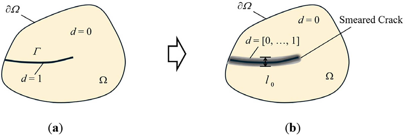
Figure 1: In a 2D phase-field damage model, a sharp crack Γ is smeared by internal length scale l0. (a) Before. (b) After

The purpose of this diffuse representation is to introduce, across the discontinuity Γ, the following approximation for the fracture surface

AΓ=∫Ωγ(d,∇d)dV,(1)

where AΓ is the crack area. The introduction of the crack density function γ circumvents the need to track discrete crack surfaces, defined as [37]

γ≈14c0[1l0o(d)+l0(∇d⋅∇d)],(2)

where the parameter c0 is to ensure that the fracture surface converges to the actual crack extension Γ0→Γ when the crack width is l0→0. o(d) is called the crack geometry function o(d)∈[0,1], which must fulfill the following relationship

o(0)=0,o(1)=1,o′(d)≥0 for 0≤d≤1.(3)

2.2 Phase-Field Framework Considering Viscous Dissipation

According to Griffith’s theory of brittle fracture, Francfort and Marigo proposed incorporating the fracture energy density into the total free energy ψ of a continuous body [38]:

ψ=ψe+ψf,(4)

where ψe and ψf denote the elastic energy density and fracture energy density during the deformation of the body, respectively.

The phase-field model established using Eq. (4) has been widely applied in studies on the fracture behavior of brittle materials. This study extends this principle, postulating that not only is elastic energy stored and contributes to accelerating damage evolution, but also that a portion of the viscous dissipation energy is stored and participates in this process:

ψ=ψe+ψv+ψf(5)

where ψv represents the viscous energy density. The expressions for each energy component will be discussed in detail in the following sections.

2.2.1 Internal Energy Density

The elastic energy density component can be expressed as:

ψe(e,d)=ω(d)ψe0(e),(6)

where e and ψe0 denote the elastic strain and the energy density in the undamaged material, respectively. ω(d) is the degradation function, used to reflect the degree of damage within the material caused by microcrack formation. Specifically, the degradation function ω(d) is introduced to account for the reduction in internal energy due to damage. It adheres to the following conditions [32]:

ω(0)=1,ω(1)=0,ω′(1)=0,ω′(d)<0.(7)

Based on the work of Shen et al. [27], we define the stored viscous energy component in the viscoelastic body as follows:

ψv(ρ,d)=(1−α)ωv(d)ψv0(ρ),(8)

where ρ and ψv0 represent a vector of strain-like viscous internal variables and the viscous energy density in the undamaged material, respectively. The dissipation factor α, ranging from [0, 1], is introduced here to quantify the influence of viscous dissipation level on the mechanical response process of the material. (1−α)ωv(d)ψv0 denotes the stored portion of viscous energy within the material during its response, while αωv(d)ψv0 represents the energy density of dissipated portion. Eq. (8) hypothesizes that the rate-dependency of viscoelastic materials is directly related to the proportion of viscous energy dissipation and storage. A specific analysis and discussion of the dissipation factor α are provided in Section 5. The degradation function ωv(d) influences the viscous energy similarly to the elastic energy degradation function. Here, ωv(d)=ω(d) is applied. However, other potentially more complex choices could be considered [39,40].

Most studies [41–43] employ ω(d)=(1−d)2 as the degradation function in phase-field models. In contrast, Borden et al. [44] used the following degradation function

ω(d)=s[(1−d)3−(1−d)2]+3(1−d)2−2(1−d)3,(9)

where s>0, for the specific meaning of s, please refer to literature [45]. Notably, the degradation function (1−d)2 is a special case of Eq. (9) when s = 2. To more comprehensively investigate the influence of the degradation function on the predictive capability of the phase-field model, we also introduce the degradation function from the phase-field cohesive zone model (CZM) [46]:

ω(d)=2(1−d)22(1−d)2+ad(2−d),(10)

where a is a material parameter related to the crack width l0. All three degradation functions listed above strictly satisfy the conditions specified in Eq. (7). Section 4.4 will provide a detailed comparison of these three degradation functions, analyzing which one is more suitable to describing the mechanical response of viscoelastic materials.

2.2.2 Fracture Energy Density

The fracture energy density of a body is usually expressed as the product of the critical energy release rate and the crack density function. According to the smeared crack surface density Eq. (2), the energy produced by crack propagation in the phase-field is

ψf(d,∇d)=Gcγ=Gc2l0d2+Gcl02|∇d|2.(11)

Here, the critical energy release rate Gc is a material parameter, defined as the energy released per unit thickness when a crack extends by one unit length. In this work, o(d)=d2 and c0=2 are defined. Next, the conditions that satisfy the thermodynamic consistency in the viscoelastic phase-field model are verified.

2.2.3 Thermodynamic Consistency and Governing Equations

In the absence of inertia, the macro-force balance law can be expressed as

∇⋅σ+b=0,(12)

where ∇⋅ is the divergence operator. σ and b are the damaged stress tensor and body force vector, respectively.

In reference to Miehe et al. [32], we postulate the existence of a microforce balance system within the body Ω. This system is characterized by an internal microforce χ and a surface force ς=ξ⋅n acting at the boundary ∂Ω. Here, ξ represents the microforce traction vector. The internal microforce and the surface microforce are conjugate to the phase-field value d and the phase-field gradient ∇d. Then the balance of microforce over the volume V is given by

∫∂ΩςdA+∫ΩχdV=0.(13)

Following a similar derivation as above, we obtain

∇⋅ξ+χ=0.(14)

The internal energy production for viscoelastic solids is given by

ρ0ℰ˙=σ:ε˙+ξ⋅∇d˙−χd˙,(15)

where ρ0 and ℰ˙ are the mass density and the entropy of the body, respectively. ε˙ denotes the rate of deformation tensor, corresponding to the time derivative of the total strain.

Let ψ˙ denote the rate of change of free energy density. In the absence of heat flux and heat sources, the Clausius–Duhem dissipation inequality states

𝒟=ρ0ℰ˙−ψ˙≥0,(16)

where ρ0 and 𝒟 represent the mass density and the total mechanical dissipation of the body, respectively.

Following the definition in Eq. (5), the rate of free energy is calculated as an additive decomposition of the elastic and viscous components of fracture, as follows

ψ˙=ψ˙e+ψ˙v+ψ˙f.(17)

Following Eqs. (6), (8), (11) and (15), we obtain

{ψ˙e=∂ψe∂e:e˙+∂ψe∂dd˙,ψ˙v=∂ψv∂ρ:ρ˙+∂ψv∂dd˙,ψ˙f=∂ψf∂∇d⋅∇d˙+∂ψf∂dd˙.(18)

Substituting Eqs. (15) and (18) into the Clausius–Duhem dissipation inequality yields

𝒟=(σ:ε−∂ψe∂e:e˙−∂ψv∂ρ:ρ˙)+(ξ−∂ψf∂∇d)⋅∇d˙−(χ+∂ψe∂d+∂ψv∂d)d˙≥0.(19)

Eq. (19) holds for any arbitrary thermodynamic process, which means that all admissible rate terms corresponding to e˙, ρ˙, ∇d˙ and d˙, must satisfy

{σ:ε≥ω(d)(∂ψe0∂e:e˙+(1−α)∂ψv0∂ρ:ρ˙),ξ=∂ψf∂∇d,χ=−∂ψe∂d−∂ψv∂d.(20)

When the constitutive relation employs a linear viscoelastic model as shown in Section 2.3, the following condition must hold

σ:ε=∂ψe0∂e:e˙+∂ψv0∂ρ:ρ˙.(21)

Given that the degradation functions satisfy 0≤ω(d),α≤1, the inequality ≥ in Eq. (20) is satisfied.

Incorporating the phase-field microforce expressions Eq. (20) into the balance law Eq. (14) yields the governing equations for the viscoelastic phase-field model

ω′(d)[ψe0+(1−α)ψv0]+Gcl0(d−l02Δd)=0, on Ω.(22)

From above discussion, it is shown that the rate of free energy in Eq. (17) satisfies the second law of thermodynamics.

Consider an initial boundary-value problem whereby governing equations are given by Eqs. (12) and (22). The boundary conditions are

∇d⋅n=0, on ∂Ω,(23)

ω(d)σ⋅n=t, on ∂Ω,(24)

u=u¯, on ∂Ω,(25)

where u¯ denotes the known displacement.

The term [ψe0+(1−α)ψv0] in Eq. (22) represents the undegraded total internal energy density, also referred to as the phase-field driving energy. During the unloading process (i.e., strain decreases) after body damage occurs, it is necessary to prevent the variable d from decreasing due to a reduction in the phase-field driving energy. Therefore, phase-field modeling must strictly enforce the irreversibility condition for the damage variable (d˙≥0), ensuring that damage evolution is either monotonically increasing or constant. To guarantee this, we introduce a history variable

ℋ={ψt if ψt>ℋn,ℋn otherwise,(26)

where ℋn is the energy value from the previous time increment. ℋ, the maximum historical value of the strain energy density, replaces the total driving energy ψt=[ψe0+(1−α)ψv0], satisfying the Karush-Kuhn-Tucker (KKT) conditions [47]

ψt−ℋ≤0,ℋ˙≥0,ℋ˙(ψt−ℋ)=0.(27)

These conditions apply to both loading and unloading.

2.3 Viscoelasticity Constitutive Relationship

This subsection focuses on the expressions for elastic energy density and viscous energy density to quantify the phase-field driving energy.

2.3.1 Generalized Maxwell Model

The constitutive relationship for viscoelastic materials is often described using rheological elements combining springs and dashpots. Based on the deviatoric-volumetric decomposition of the stress tensor, this work introduces a Generalized Maxwell Model (GMM), as illustrated in Fig. 2. The model consists of separate parts for the deviatoric stress (σdev) and the volumetric stress (σvol ). Each part contains one equilibrium branch (a spring) and multiple non-equilibrium branches (each a Maxwell model: a spring in series with a dashpot).

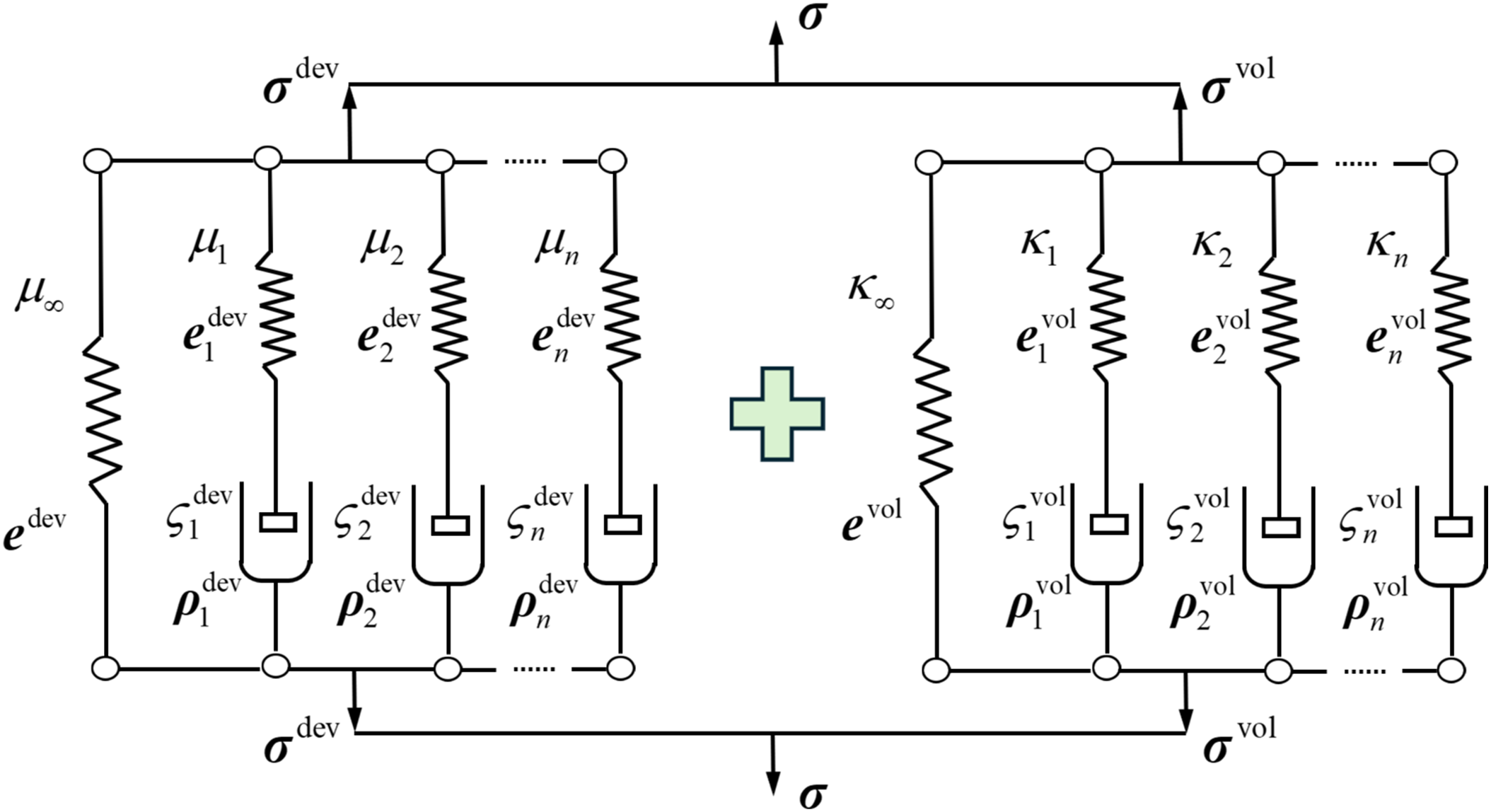
Figure 2: Schematic representation of the generalized Maxwell model

Consequently, the strain tensor can also be decomposed into a deviatoric strain tensor (edev) and a volumetric strain tensor (evol), summing as

ε=edev+evol,(28)

where evol=1/3tr(ε)I, tr(ε) is solved according to the Einstein summation convention, and I represents the second-order identity tensor.

Within an individual non-equilibrium branch, the strain is expressed as

edev=emdev+ρmdev,(29)

evol=emvol+ρmvol,(30)

where m satisfies 1 ≤ m ≤ n, and n is the total number of non-equilibrium branches. emdev and ρmdev denote the elastic strain of the spring and the viscous strain of the dashpot, respectively, in the mth non-equilibrium branch of the deviatoric part. Similarly, emvol and ρmvol denote the same for the volumetric part.

Analogously, the stress tensor obeys the relation σ=σdev+σvol. According to the schematic in Fig. 2, σdev and σvol are given by

σdev=σ∞dev+∑m=1nσmdev,(31)

σvol=σ∞vol+∑m=1nσmvol.(32)

Here, σ∞dev and σ∞vol represent the stresses in the equilibrium branches, while σmdev and σmvol represent the stresses in the mth non-equilibrium branch.

The stress-strain relation of the equilibrium branch is

σ∞dev=2μ∞edev,(33)

σ∞vol=3κ∞evol,(34)

where μ∞ and κ∞ are the shear modulus and bulk modulus of the equilibrium branch.

Crucially, because the stress in the dashpot equals the stress in the spring within the mth Maxwell branch, the stress-strain relation of each non-equilibrium branch is

{σmdev=2μmemdev=ζmdevρ˙mdev,σmvol=3κmemvol=3ζmvolρ˙mvol,(35)

where the dot superscript (˙) denotes the derivative with respect to time t. μm and κmare the shear modulus and bulk modulus of the mth non-equilibrium branch, respectively. ζmdev and ζmvol are the volume viscosity and shear viscosity of the mth non-equilibrium branch, respectively.

The basic hereditary integral formulation for linear isotropic viscoelasticity is

σ(t)=∫0t2μ(t−τ)dedevdτdτ+I∫0tκ(t−τ)devoldτdτ.(36)

In the generalized Maxwell model depicted in Fig. 2, the relaxation functions κ(t) and μ(t) can be individually defined as a series of exponentials, known as the Prony series

μ(t)=μ∞+∑m=1nμme−t/τmdev,(37)

κ(t)=κ∞+∑m=1nκme−t/τmvol,(38)

where τmdev and τmvol are the deviatoric relaxation time, and volumetric relaxation time, respectively, of the mth non-equilibrium branch. The relaxation times are expressed as:

τmdev=ςmdev/μm,(39)

τmvol=ςmvol/κm.(40)

2.3.2 Elastic Energy and Viscous Energy

Based on the decomposition form of the generalized Maxwell model, the elastic energy density ψe0 can be expressed as

ψe0=(ψedev)∞+(ψevol)∞+∑m=1n[(ψedev)m+(ψevol)m],(41)

here, (ψedev)∞ and (ψevol)∞ represent the deviatoric and volumetric elastic energy densities of the equilibrium branch in the generalized Maxwell model. (ψedev)m and (ψevol)m denote the deviatoric and volumetric elastic energy densities of the mth non-equilibrium branch, respectively, defined as

{(ψedev)∞=μ∞edev:edev(ψedev)m=μmemdev:emdev,(42)

{(ψevol)∞=12κ∞[tr(evol)]2(ψevol)m=12κm[tr(emvol)]2,(43)

similar to the elastic energy density, the total viscous dissipation energy density ψe0 is expressed as

ψe0=ψvdev+ψvvol=∑m=1n[(ψvdev)m+(ψvvol)m].(44)

where the total viscous dissipation energy density is split into deviatoric ψvdev and volumetric ψvvol components. (ψvdev)m and (ψvvol)m represent the deviatoric and volumetric viscous dissipation energy densities for the mth non-equilibrium branch, given by

{(ψvdev)m=ςmdev∫0tρ˙mdev:ρ˙mdevdτ,(ψvvol)m=ςmvol∫0tρ˙mvol:ρ˙mvoldτ.(45)

Although Eq. (45) defines the dissipation energy density, numerical solution is complicated by the presence of viscous strain rates ρ˙mdev and ρ˙mvol [22,27]. Substituting Eq. (35) into Eq. (45) transforms the viscous energy density expression into a non-viscous-strain-rate form

{(ψvdev)m=(2μm)2ςmdev∫0temdev:emdevdτ,(ψvvol)m=(κm)2ςmvol∫0t[tr(emvol)]2dτ.(46)

Introducing the relaxation times τmdev, τmvol and using Eqs. (39) and (40), this equation can be rewritten as:

{(ψvdev)m=2μmτmdev∫0temdev:emdevdτ,(ψvvol)m=κmτmvol∫0t[tr(emvol)]2dτ.(47)

Combining Eqs. (42), (43), and (47) further yields

{(ψ˙vdev)m=2τmdev(ψedev)m,(ψ˙vvol)m=2τmvol(ψevol)m,(48)

where (ψ˙vdev)m and (ψ˙vvol)m are the rates of the deviatoric and volumetric viscous dissipation energy densities for the mth non-equilibrium branch, respectively. Additionally, we assume τm=τmdev=τmvol in this work.

3  Numerical Discretization and Acceleration Scheme

Next, we formulate the weak form, linearize and discretize our model. Special attention is paid to the treatment of the adaptive time-stepping in the staggered scheme.

3.1 Weak Formulation and Finite Element Implementation

Based on the Galerkin method, the proposed phase-field framework is numerically discretized to derive the global tangent stiffness matrix for the iterative calculations of finite element. First, the phase-field microscopic force balance Eq. (22) and the macroscopic force balance Eq. (12) are multiplied by the trial functions wd and wu, respectively. These are then integrated over the problem domain, and integration by parts is applied to obtain the weak forms of the phase-field residual equation and the displacement field residual equation for a single element

Rue=∫Ω∇wuT:σdV−∫ΩwuT⋅bdV−∫ΓwuT⋅tdS,(49)

Rde=∫Ω[Gcl0∇wdT∇d+∂ω(d)∂dψtwd+Gcl0dwd]dV.(50)

The solution spaces for the displacement field, 𝒮u, and the phase-field, 𝒮d, are defined as follows:

𝒮u={u∣u∈H1,u=u¯ on ∂Ω},(51)

𝒮d={d∣d∈H1},(52)

where H1 represents the first-order Sobolev space [48]. The solution spaces for the trial functions are:

𝒱u={wu∣wu∈H1,wu=0 on ∂Ωu},(53)

𝒱d={wd∣wd∈H1}.(54)

For a single mesh element, the finite element discretization of the displacement trial function, the phase-field trial function, and their corresponding gradients can be expressed as:

wu=Nuue,∇wu=ε=Buue,(55)

wd=Ndde,∇wd=Bdde.(56)

Here, ue and de are the nodal displacement vector and nodal phase-field vector, Nu and Nd are the element shape function matrices for the displacement and phase-fields, respectively, and Bu and Bd are the element geometric function matrices. In code implementation, standard bilinear or trilinear shape functions N are used for both displacement and phase-field variables.

Following standard finite element procedures, assembly yields the global equations

Ru=0,Rd=0.(57)

Eq. (57) forms a coupled nonlinear residual equation system between the displacement and phase-fields, typically requiring an iterative solution. The coupled iterative solution of displacement and phase-fields is termed the monolithic scheme [32].

The staggered scheme is adopted here. The specific solution process from time tl to tl+1 is carried out through the following three steps:

a.   Determine the current ℋn with the displacement variable u at time tl.

b.   With the ℋn to update the phase-field variable d at time tl+1 based on Eq. (50).

c.   With the phase-field value d calculated in the previous step to solve the displacement variable u at time tl+1 based on Eq. (49).

The Newton-Raphson method is used for iterative calculation. Let ul and dl denote the displacement and phase-field values, respectively, at the lth iteration within the kth timestep. The format for the (l + 1)th iteration is then

{dl+1ul+1}={dlul}+[Kldd00Kluu]−1{RldRlu},(58)

Here, the off-diagonal coupling tangent stiffness matrix terms Klud and Kldu are omitted. Kldd and Kluu represent the tangent stiffness matrices for the phase-field and displacement field, respectively. The first letter in the superscript identifies the residual component, while the second letter indicates the partial derivative with respect to the solution variables ul and dl. These matrices are obtained by assembling theωir respective elemental tangent stiffness matrices

Kedd=−∂Rde∂de=∫ΩGcl0⁢[(Nd)T⁢Nd+l02⁢(Bd)T⁢Bd]dV+∫Ωω′′⁡(d)⁢ψt⁢(Nd)T⁢NddV,(59)

Keuu=−∂Rue∂ue=∫Ωω(d)(Bu)TDBudV,(60)

where D is the stiffness matrix. The primary advantage of the above-mentioned staggered scheme compared to the monolithic scheme is that it has a relatively high numerical robustness, which is more necessary particularly when the phase-field variable evolves rapidly. However, load increments must be sufficiently small within this staggered scheme to achieve adequate numerical accuracy [49].

3.2 Discretization of the Generalized Maxwell Model

To enable stress calculation within the finite element framework, the incremental forms for deviatoric strain, deviatoric stress, elastic energy, and viscous dissipation energy are derived below. The derivations for volumetric strain, volumetric stress, volumetric elastic energy, and volumetric viscous dissipation energy follow a similar process.

The deviatoric integral equation is

σdev=∫0t2(μ∞+∑m=1nμme(t−τ)/τmdev)dedevdτdτ.(61)

We rewrite this equation in the form

σdev=2μ0(edev−∑m=1nξmρmdev),(62)

where μ0=μ∞+∑m=1nμm is the instantaneous shear modulus. ξm=μm/μ0=κm/κ0 is the normalized form of the shear modulus. According to Eq. (36) and the strain relationship between the spring and dashpot, the viscous strain ρmdev, in the mth non-equilibrium branch, can be expressed as

ρmdev=∫0τ(1−e(τf−τ)/τmdev)dedevdτfdτf.(63)

For finite element analysis this equation must be integrated over a finite increment of time. To perform this integration, we will assume that edev varies linearly with τ during the increment; hence, dedev/dτf=Δedev/Δτ. To use this relation, we break up Eq. (63) into two parts

(ρmdev)l+1=∫0τn(1−e(τf−τl+1)/τmdev)dedevdτfdτf+∫τnτn+1(1−e(τf−τl+1)/τmdev)dedevdτfdτf.(64)

Now observe that

1−e(τf−τl+1)/τmdev=1−e−Δτ/τmdev+e−Δτ/τmdev(1−e(τf−τl)/τmdev).(65)

Use of this expression and the approximation for dedev/dτf during the increment yields

(ρmdev)l+1=(1−e−Δτ/τmdev)∫0τldedevdτfdτf+e−Δτ/τmdev∫0τl(1−e(τf−τl)/τmdev)dedevdτfdτf+ΔedevΔτf∫τlτl+1(1−e(τf−τl+1)/τmdev)dτf.(66)

The first and last integrals in this expression are readily evaluated, whereas from Eq. (63) follows that the second integral represents the viscous strain in the mth non-equilibrium branch at the beginning of the increment. Hence, the change in viscous strain is

Δρmdev=(ρmdev)l+1−(ρmdev)l=(1−e−Δτ/τmdev)(edev)l+(e−Δτ/τmdev−1)(ρmdev)l+(Δτ−τmdev(1−e−Δτ/τmdev))ΔedevΔτf.(67)

Eq. (62) is then used subsequently to obtain the new value of the stresses

Δσdev=(σdev)l+1−(σdev)l=2μ0(edev−∑m=1nξm((ρmdev)l+1−(ρmdev)l)).(68)

The tangent modulus, depends only on the reduced time step, is readily derived from these equations by differentiating the deviatoric stress increment, which is

μ=μ0[1−∑m=1nξmτmdevΔτ(Δττmdev+e−Δτ/τmdev−1)].(69)

When a strain increment Δe occurs in the deviatoric stress branch of the generalized Maxwell model, the increment of the total strain energy in the branch is

ΔWTotdev=(σdev)l:Δedev+12((σdev)l+1−(σdev)l):Δedev=12(((σdev)l+1+(σdev)l):Δedev.(70)

Similarly, when a viscous strain increment ξmΔρmdev occurs in the mth non-equilibrium branch, the increment of viscous dissipation energy for the deviatoric part of the generalized Maxwell model is

ΔWvdev=(σdev)n:∑m=1nξmΔρmdev+12((σdev)n+1−(σdev)n):∑m=1nξmΔρmdev=12((σdev)n+1+(σdev)n):∑m=1nξmΔρmdev.(71)

The increment of elastic energy can be expressed as

ΔWedev=ΔWTotdev−ΔWvdev.(72)

Following the same steps outlined from Eqs. (61)–(72), the corresponding expressions for the volumetric part of the generalized Maxwell model can be derived.

The numerical discretization within the finite element framework is implemented using Abaqus [50] user subroutines: User element subroutine (UEL) for the main phase-field framework program, User-defined material subroutine (UMAT) for visualizing results from the phase-field framework computations, and Abaqus main control routine (ABQMAIN) for post-processing of calculated data.

3.3 Adaptive Time-Stepping Scheme

As mentioned above, staggered algorithms for solving coupled displacement-phase-field problems necessitate sufficiently small, constant load increments to ensure accuracy. This fixed time-stepping approach inevitably leads to significant computational expense, particularly for complex structures or large-scale models. To preserve the robustness of the staggered scheme while substantially reducing computation time in Abaqus, this section introduces an adaptive time-stepping strategy.

The core principle of adaptive scheme is to dynamically adjust the time increment by identifying critical states in phase-field evolution. The theoretical basis stems from Miehe’s [51] alternative form of fracture energy

Wf=∫Ω[W0(d)+r(d)]dV,(73)

where W0(d) represents the function of fracture energy. r(d) serves as a critical threshold in phase-field modeling, defined as

r(d)=ϕc[1−ω(d)],(74)

with ϕc being the specific fracture energy governing damage initiation.

We let ϕc=Gc/2l0, resulting in a fracture energy expression

W0(d)=Gc∫Ωγ(d,∇d)dV=∫ΩGc2l0[d2+l02|∇d|2]dV,(75)

consistent with Eq. (11).

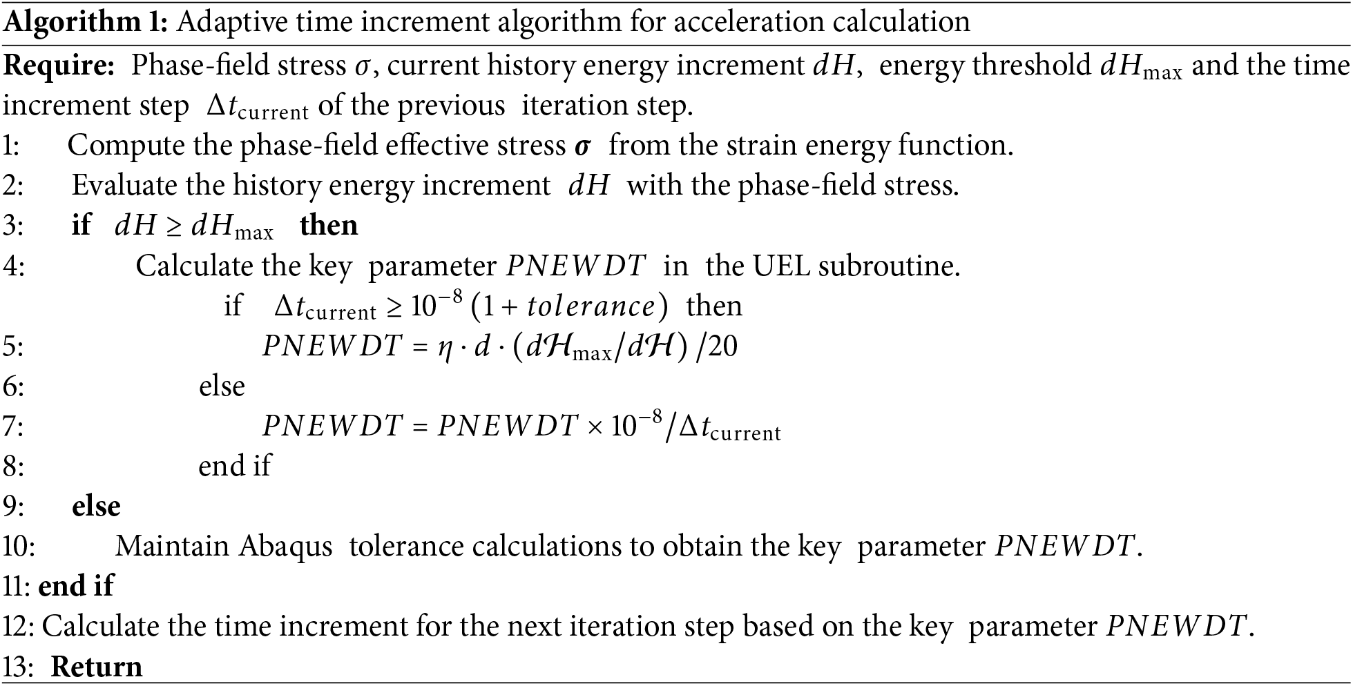
The adaptive time stepping operates as follows: When the driving energy dℋ computed at lth increment remains below dℋmax, the time increment for step l + 1 is increased according to the default tolerance-based scheme of Abaqus. This leverages Abaqus’ inherent tendency to maximize increments when convergence and accuracy permit, enhancing efficiency away from fracture zones. Conversely, if dℋ equals or exceeds dℋmax, the algorithm reduces the subsequent increment according to the rules prescribed in Algorithm 1. Here, dℋ=ℋn+1−ℋn.

The threshold dℋmax is set as

dℋmax=ϕc/10=Gc20l0,(76)

ensuring refined time increments near critical energy states.

We validate the effectiveness of our adaptive time-stepping scheme using a typical benchmark: simulating fracture in a single-edge notched square plate. The model features a prefabricated horizontal crack extending from the left surface to the geometric center, with geometry, boundary conditions, and loading depicted in Fig. 3. The bottom surface is fixed, while a constant vertical displacement rate (0.01 mm/s) is applied to the top surface to simulate quasi-static tensile loading. To accurately capture fracture, a fine mesh (element size down to h = 1.0 × 10−3 mm) is used in the central region. The model, discretized into 25,292 quadrilateral elements, employs material parameters from Ref. [37]: Young’s modulus E = 210 GPa, Poisson’s ratio ν = 0.3, phase-field length scale l0 = 0.0075 mm, and critical energy release rate Gc = 2.7 N/mm.

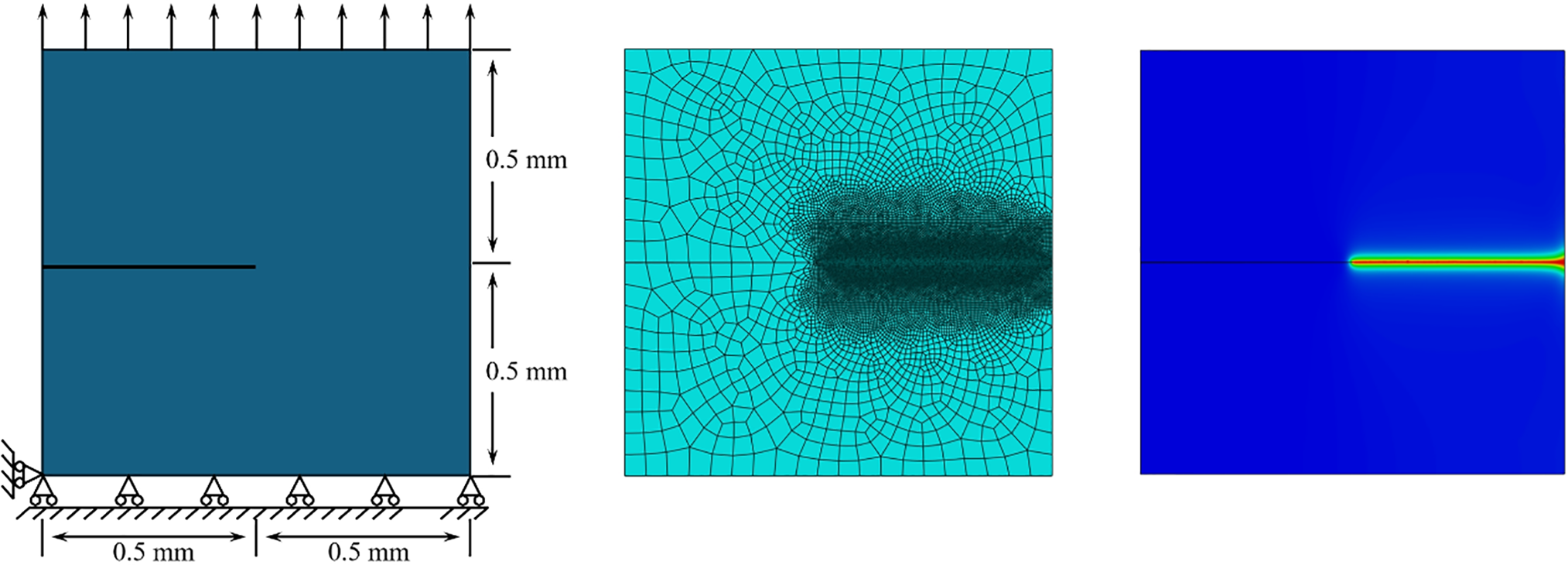
Figure 3: The plate geometry, mesh, and computed phase-field contours using the adaptive scheme

The initial time increment is 0.1 s, and subsequent steps are dynamically determined by Algorithm 1. For comparison, four time-step strategies are implemented: (1) ∆t = 0.1 s; (2) ∆t = 0.01 s; (3) ∆t = 0.001 s; (4) A fixed two-stage increment scheme: ∆t = 0.001 s up to a displacement of 0.004 mm (identified from preliminary analysis), switching to ∆t = 0.0001 s afterwards to better resolve fracture progression.

Fig. 4a compares the load-displacement curves. Our adaptive scheme’s result closely matches the solution from Miehe et al. [37]. Fig. 4b compares normalized computation times. The adaptive scheme requires only about 1/6.5 of the time taken by the two-stage fixed scheme (0.001 s + 0.0001 s), demonstrating significant efficiency gains.

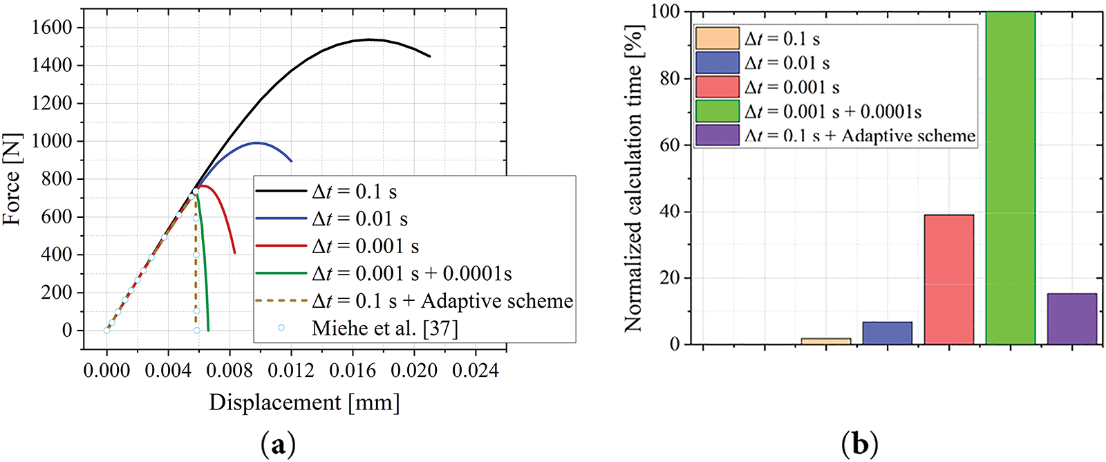
Figure 4: Tensile simulation results for the single-edge notched square plate [37]. (a) Force-displacement responses of all schemes. (b) Normalized computation time for all schemes

Therefore, the adaptive scheme not only reduces computational time but also enhances usability. It eliminates the manual intervention required in the two-stage fixed scheme (specifically switching to a fine step size to capture fracture), streamlining the simulation workflow.

4  Parameter Identification of Viscoelastic Phase-Field Model

In this section, experimental datasets from the mechanical testing of solid propellants are employed to identify unknown parameters within the established phase-field framework. These include phase-field fracture parameters and viscoelastic parameters of the generalized Maxwell model. Additionally, data from tensile tests under varied strain rates are also used to prepare for the validation of the phase-field framework in Section 5.1.3.

4.1 Experiments

The following two types of tests employed a hydroxyl-terminated polybutadiene (HTPB) composite propellant with filler particles comprising 88% of the mass. In this filler fraction, ammonium perchlorate (AP) and aluminum (Al) accounted for mass fractions of 70% and 18%, respectively.

4.1.1 Tensile Relaxation Test of Solid Propellant

Following method of the American JANNAF (Joint Army-Navy-NASA-Air Force) standard [52], uniaxial tensile tests are performed on the propellant under constant strain. The time-dependent relaxation force is measured during the relaxation process, allowing calculation of the tensile relaxation modulus at various time points. By applying the Time-Temperature Superposition Principle (TTSP), the relaxation modulus curves obtained at different temperatures are shifted to construct the master curve of stress relaxation modulus at a reference temperature (typically room temperature). This data provides the foundation for identifying parameters of the Generalized Maxwell Model, discussed in the next section.

The geometry and dimensions of the test specimen are shown in Fig. 5. Relaxation tests are performed using a universal testing machine (UTM) equipped with an environmental chamber. Specimens are stretched at a constant rate of 0.12 s−1 (equivalent to the speed of 500 mm/min) to an initial engineering strain of 5% (3.5 mm). This strain level is then held constant while the stress decay is continuously monitored for a duration of 1000 s. Tests are conducted across six temperature conditions: 70°C, 50°C, 20°C, 0°C, −20°C, and −40°C. Prior to testing, the gauge length between fixtures is set to 70 mm, and a slight preload tension is applied to eliminate any slack. Specimen displacement is recorded using the UTM’s high-precision built-in sensors. Furthermore, propellant specimens are conditioned in the environmental chamber for 30 min before each test at a specific temperature to ensure thermal equilibrium.

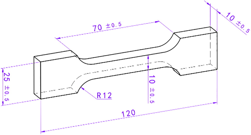
Figure 5: Dogbone sample size of solid propellants

The initial cross-sectional area of each specimen is measured at multiple points using vernier calipers before testing to calculate the relaxation modulus. To minimize variations between individual samples, three identical specimens are tested in parallel at each set temperature, and their results are averaged. To account for initial instabilities in the test process, data collection commenced at the 2-s mark. Analysis focused on relaxation data at the following eleven specific time points: 2, 4, 8, 20, 40, 80, 120, 200, 400, 800, and 1000 s. The resulting tensile stress relaxation modulus curves for the HTPB propellant at various temperatures are shown in Fig. 6.

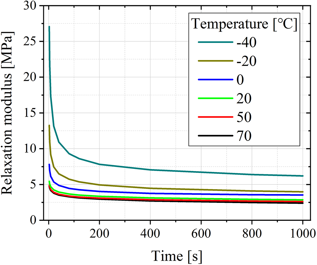
Figure 6: Relaxation modulus-time curves at different temperatures

4.1.2 Constant-Rate Tensile Testing of Solid Propellant

The constant-rate tensile testing of the HTPB propellant is conducted in accordance with ASTM D638 [53]. Specimens maintained the dogbone geometry and dimensions shown in Fig. 6, with an engineering gauge length of 70 mm. The constant-rate tensile testing is also carried out on the universal testing machine, employing the same fixtures as those used in the tensile relaxation tests. The primary purpose of this test is to acquire data to calibrating the fracture parameters (specifically, the characteristic length l0 and the critical energy release rate Gc). The test employs four tensile rates: 10, 100, 500, and 1000 mm/min, with four parallel specimens tested.

Among them, the 1000 mm/min rate test data is used to identify the fracture parameters for the proposed viscoelastic phase-field model. The three sets of test data at 10, 100, and 500 mm/min are used for model validation in Section 5.1.3.

4.2 Parameter Identification of the Generalized Maxwell Model

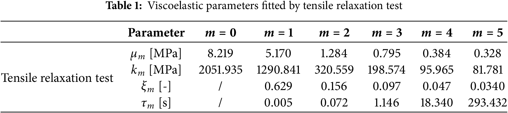
As illustrated in Fig. 2, the generalized Maxwell model is decomposed into deviatoric and volumetric components. Essentially, each individual part can be viewed as a Prony series. Previous research has established that the number of terms (m) within the Prony series significantly impacts the accuracy of material response simulations and analysis. A minimum of m = 5 terms is required for a Prony series to accurately capture the linear viscoelastic deformation behavior of materials [54]. Consequently, given the characteristic viscoelastic behavior of HTPB propellant, the generalized Maxwell model is defined as a 5th-order series in the subsequent parameter identification work.

Leveraging the time-temperature superposition principle and the least squares method, the tensile stress relaxation modulus curves of the HTPB solid propellant at various temperatures can be shifted and subsequently fitted to construct a master tensile relaxation modulus curve, as shown in Fig. 7.

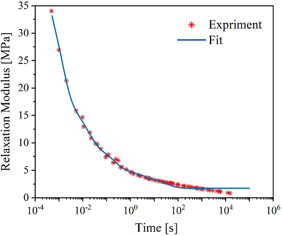
Figure 7: Relaxation modulus master curve fitting results

The specific steps are as follows:

•   Reference temperature selection: A reference temperature of T0 (20°C) is selected. The horizontal axis (time) of the relaxation modulus curves is converted to a logarithmic scale (lg⁡t), and the vertical axis is calculated as lg⁡[E−(t)⋅T0/T] to generate the lg⁡[E−(t)⋅T0/T]−lg⁡t curve.

•   Shift factor calculation: The temperature- and time-dependent shift factor αT is computed for each temperature. The logarithm of the shift factor (lg⁡αT) is then determined.

•   Curve superposition: The logarithmic curves at other temperatures are horizontally shifted and superimposed onto the reference temperature curve. A master relaxation modulus curve is subsequently obtained by applying an exponential transformation (anti-logarithm) to the shifted data.

•   Prony series fitting: Using the master curve, the relaxation coefficients of the Prony series are fitted via the least-squares method as shown in Table 1. The initial modulus and equilibrium modulus of the HPBT propellant are determined to be 24.624 and 0.911 MPa, respectively.

4.3 Identification of Phase-Field Parameters

Based on the constant-rate tensile test data, the least squares method is applied to fit fracture parameters of phase-field model. The minimized residual is defined as

ℛ=∑i=1n(Fi, test −Fi, numFi, test )2,(77)

where Fi, test  represents the measured force at the ith displacement point and Fi, num is the numerical calculated force from the viscoelastic phase-field framework.

The numerical model replicates the geometry of the dogbone specimen (Fig. 5). The boundary conditions and loading conditions used are same as in experiments. The left end of the specimen is fixed while its right end is stretched at 1000 mm/min rate. A structured hexahedral mesh with 85,176 nodes and 78,125 elements is employed, as shown in Fig. 8. Each node features four degrees of freedom: one phase-field damage variable and three displacement variables. Mesh refinement is implemented in the central potential fracture zone to enhance accuracy, achieving a minimum element size h = 0.4 mm. Numerical simulations utilized an initial constant timestep of 0.01 s prior to activating the adaptive time stepping algorithm. Material viscoelastic parameters are detailed in Table 1. Force data is extracted from the loading point.

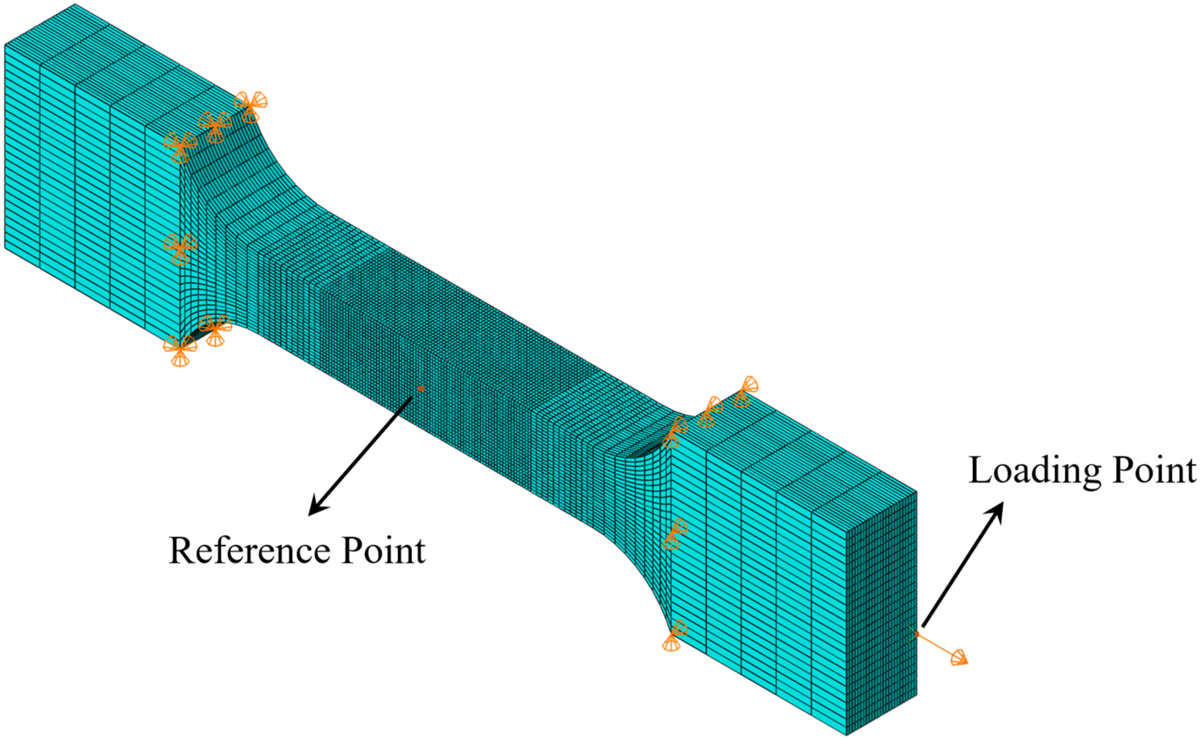
Figure 8: The mesh and boundary conditions of the dogbone specimen

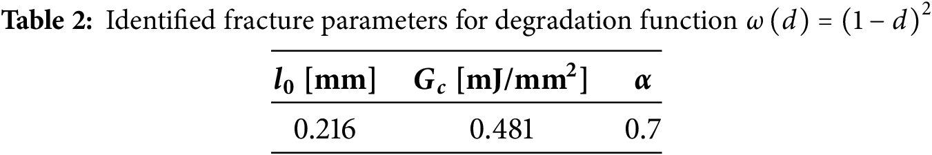
The Nelder-Mead simplex algorithm minimized the residual of Eq. (77) to perform parameter fitting. The resulting fracture parameters are summarized in Table 2.

4.4 Influence of Degradation Function

The specific form of the degradation function ω(d) is a crucial parameter in phase-field modeling, significantly influencing the accuracy of material behavior predictions, as highlighted by Sargado et al. [55] and Kuhn et al. [56]. Different choices of ω(d) directly impact the computed simulation results.

To systematically analyze this effect, we compare the three types of degradation functions discussed in Section 2.2.1:

{ω(d)1=(1−d)2,ω(d)2=m[(1−d)3−(1−d)2]+3(1−d)2−2(1−d)3,ω(d)3=2(1−d)22(1−d)2+ad(2−d),(78)

where the value m of the polynomial degradation function ω(d)2 is 1 to investigate the coupling effect of the cubic term and the quadratic term; the value a of the cohesive degradation function is 4 to investigate the influence of the typical cohesive degradation function on the viscoelastic phase-field framework calculation.

4.4.1 The Influence on One Element Tensile

One 2D plane strain element is the simplest case, where the influence of degradation function can be understood. The boundary conditions are shown in Fig. 9. The dimensions of the element are 1 mm × 1 mm. The bottom nodes are constrained in both x and y direction, whereas we allow the top nodes to slide vertically.

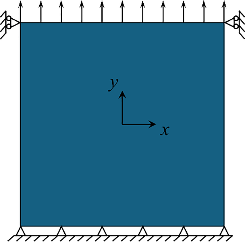
Figure 9: Geometry and boundary conditions for one element

An analytical solution exists for this constrained case. The phase-field is homogeneous (∇d = 0). Therefore, if a simple well determined deformation scheme is assumed: εx=0, γxy=0, the elastic potential energy can be calculated directly

ℋ=maxτ∈[0,t]{ψt(ε)}=maxτ∈[0,t]{12c22εy2},(79)

where c22 is the (2, 2) element of the plane strain stiffness matrix, expressed as

c22=E(1−ν)(1+ν)(1−2ν).(80)

Solving the phase-field Eq. (22) yields d depending on the chosen ω(d). For example, using the quadratic degradation function ω(d) gives

d=2ℋ2ℋ+Gc/l0,(81)

which leads to the true stress in the y direction as follows

σy=(1−d)2σ¯y=(1−d)2c22εy,(82)

where σ¯y is the undegraded stress.

The comparison between analytical and numerical solutions for each degradation function is depicted in Fig. 10a. In this comparison, the characteristic width of the phase-field is set as l0=0.1 mm. Furthermore, Fig. 10b illustrates the relationship between degradation values and phase-field values for each degradation function in this case.

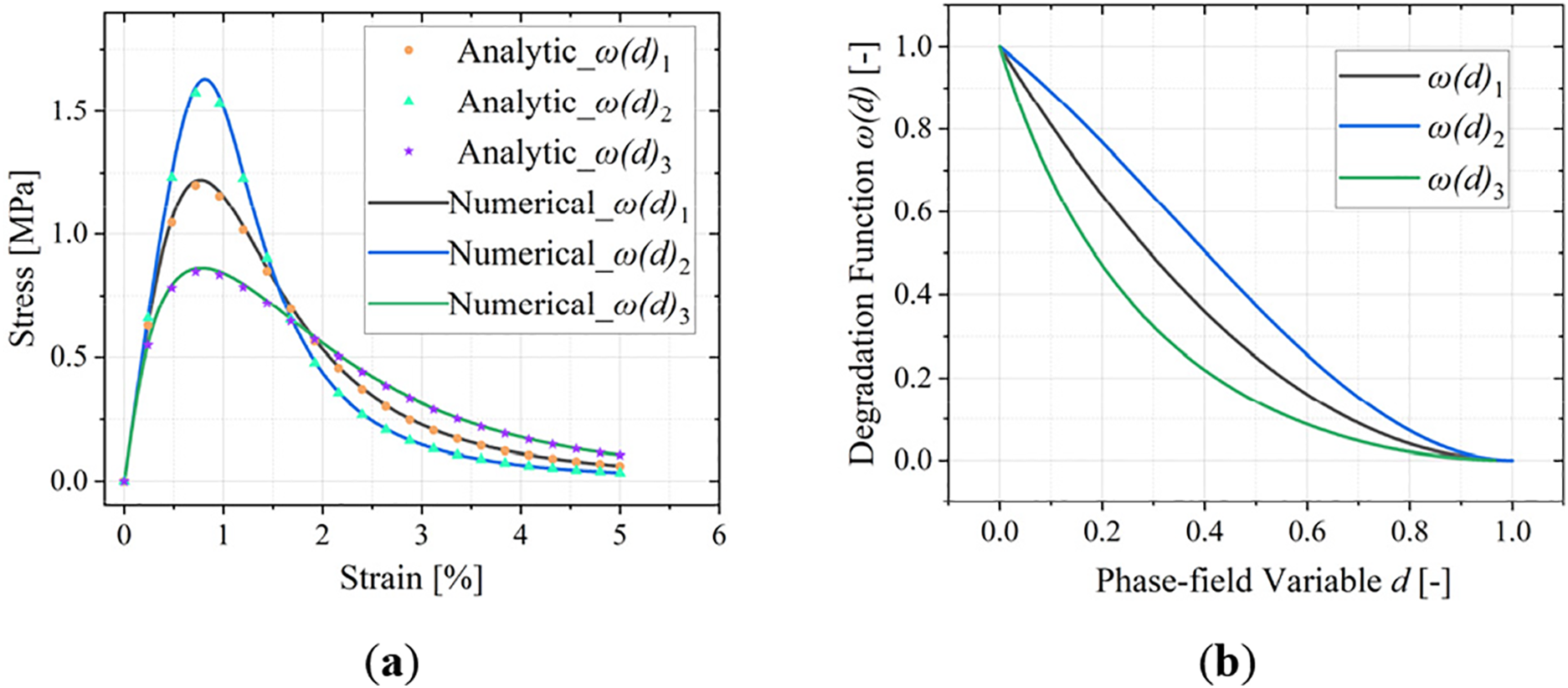
Figure 10: (a) Stress-strain relationship between analytical and numerical solutions. (b) Evolution relationship between degradation functions and damage values

Through observation in Fig. 10a, it is noted that

•   The polynomial degradation function ω(d)2 produces a more distinct initial linear elastic response compared to the quadratic ω(d)1 and cohesive ω(d)3 functions, which exhibit earlier nonlinearity.

•   The polynomial function ω(d)2 exhibits a sharper stress drop at peak stress, implying a more brittle material response relative to the quadratic and cohesive functions.

•   Degradation functions ω(d)1 and ω(d)3 lead to a slower stress decay towards zero than ω(d)2, indicating a more ductile post-peak response.

•   The strain at peak stress differs significantly between all three degradation functions. This demonstrates that the choice of ω(d) critically affects the predictions of the phase-field model on key material properties, including ultimate strength and maximum elongation.

Based on these comparative results, the quadratic ω(d)1 and cohesive ω(d)3 degradation functions appear more suitable for coupling phase-field modeling with viscoelastic material behavior.

4.4.2 The Influence on Dogbone Specimen Tensile

We also analyzed the influence of selection of degradation function on the tensile simulation of a dogbone specimen. The model geometry and boundary conditions matched those detailed in Fig. 8. Fracture parameters (internal length scale l0 and critical energy release rate Gc, see Tables 3 and 4) for degradation functions 2 and 3 are determined through residual least-squares fitting as described in Section 4.3. The comparative results in Fig. 11 demonstrate that simulations using the quadratic degradation function achieved the closest match to experimental data.

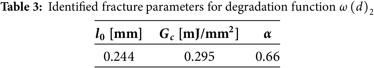
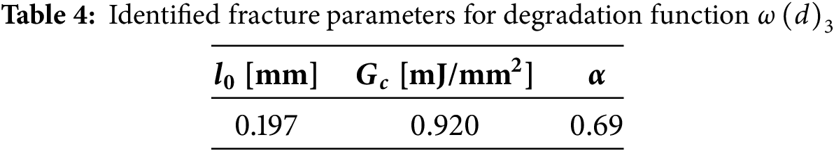
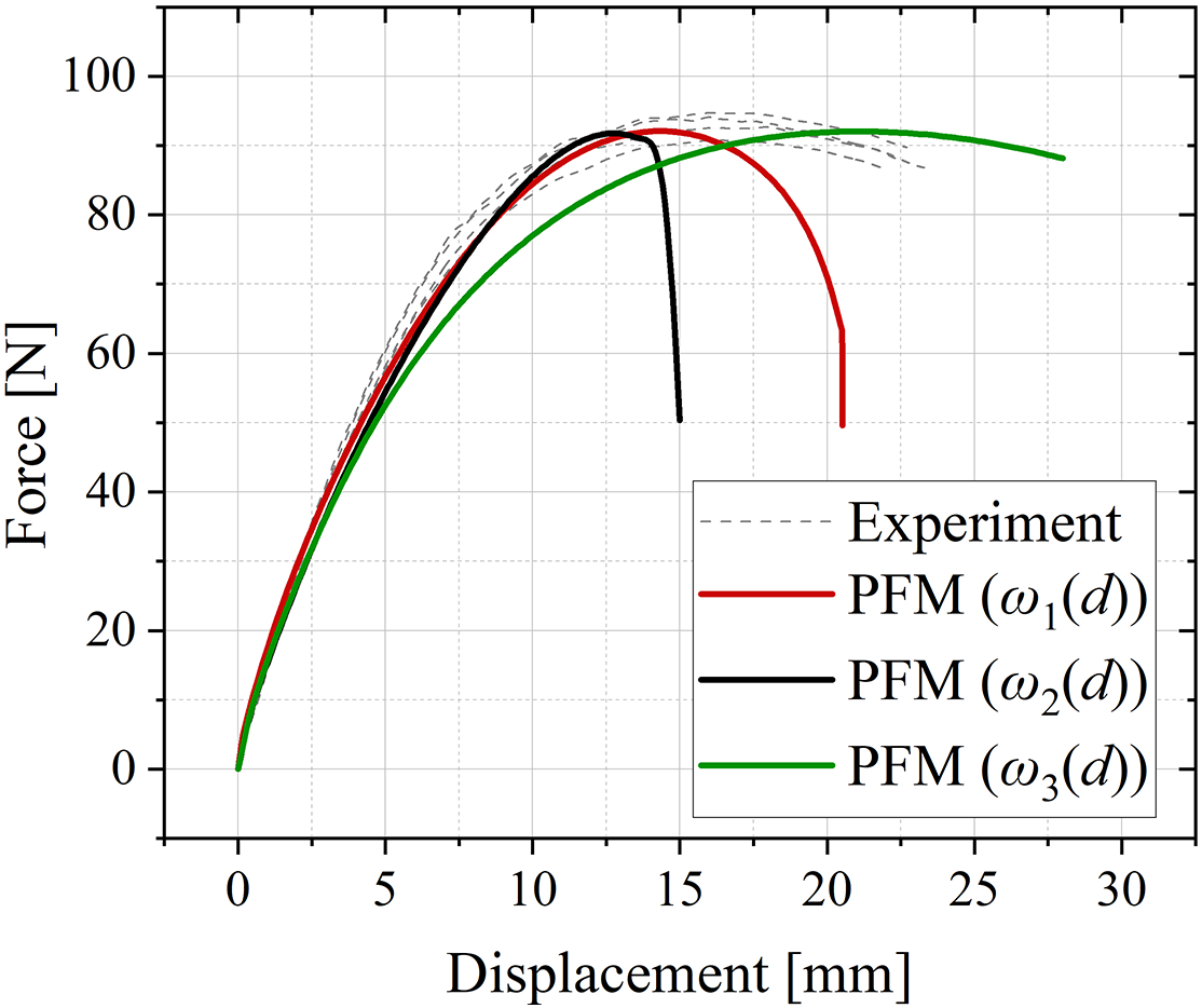
Figure 11: The influence of degradation functions on dogbone specimen tensile

Therefore, based on these findings, the quadratic degradation function is selected for all subsequent simulations in this study.

5  Simulation Analysis of the Influence of Viscous Energy Dissipation Rate

This section evaluates the ability of the developed viscoelastic phase-field framework to simulate the tensile mechanical properties and fracture behavior of solid propellants. Several numerical simulations are performed: cyclic loading, stress relaxation, constant-rate tensile fracture of dogbone samples, and tensile tests on three-dimensional single-notched plates for both Mode I (opening) and Mode II (sliding) fracture. These simulations utilize the scaling factor (α) to elucidate the intrinsic relationship between viscous dissipation and the rate-dependent damage behavior of the material. Simulations involving crack growth in structures with preexisting cracks under quasi-static loads verify the model’s capability to capture and characterize complex fracture patterns in viscoelastic materials.

5.1 Dogbone Samples Under Various Loading Conditions

5.1.1 Cyclic Loading Simulation

The cyclic loading of solid propellant is simulated using the dogbone model shown in Fig. 8. The viscoelastic constitutive parameters are listed in Table 1, while the phase-field parameters are given in Table 2, Poisson’s ratio ν = 0.498. As illustrated in Fig. 12a, a two-stage loading protocol is applied at the loading point. The first stage (before 1 s) stretched the sample at 500 mm/min to a deformation of 8.4 mm (12% stretch ratio relative to the gauge length). This is followed by a second stage involving cyclic loading with a sinusoidal variation

u(t)=Asin⁡(ωt),(83)

where the amplitude A is 2.8 mm (4% stretch ratio), with a period of 2 s (angular frequency ω = π rad/s). Notably, the first stage of loading ensures the sample avoids compression during the cycles, maintaining exclusively tensile (non-negative) stress.

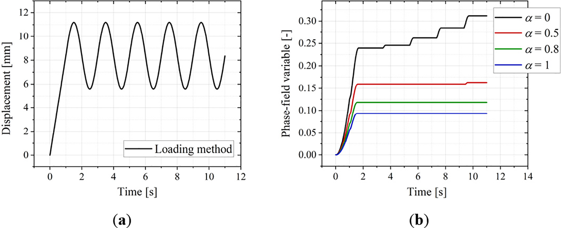
Figure 12: (a) The loading method in cyclic simulation. (b) Phase-field value evolution over time

Four different computational conditions are implemented: (1) α = 1: All viscous energy is dissipated during the material response and does not contribute to damage evolution. (2) α = 0.8: 80% viscous energy dissipates, 20% is stored. (3) α = 0.5: Viscous energy dissipation and storage are balanced. (4) α = 0: Energy is completely stored and drives damage evolution (no dissipation). Strain, stress, phase-field value, and energy results are extracted at the reference point (Fig. 8) within the dogbone model’s gauge section.

Results presented in Fig. 13 show that as the dissipation factor (α) decreases: the maximum strain amplitude in Fig. 13a gradually increases (hardening effect—see black arrow), while the maximum stress amplitude in Fig. 13b gradually decreases (softening effect). This demonstrates that the viscoelasticity of the solid propellant is intrinsically linked to the magnitude of the viscous driving energy defined in the phase-field model (Eq. (22)). Lower α (more stored energy) leads to greater viscous driving energy, The material’s viscous response becomes more pronounced.

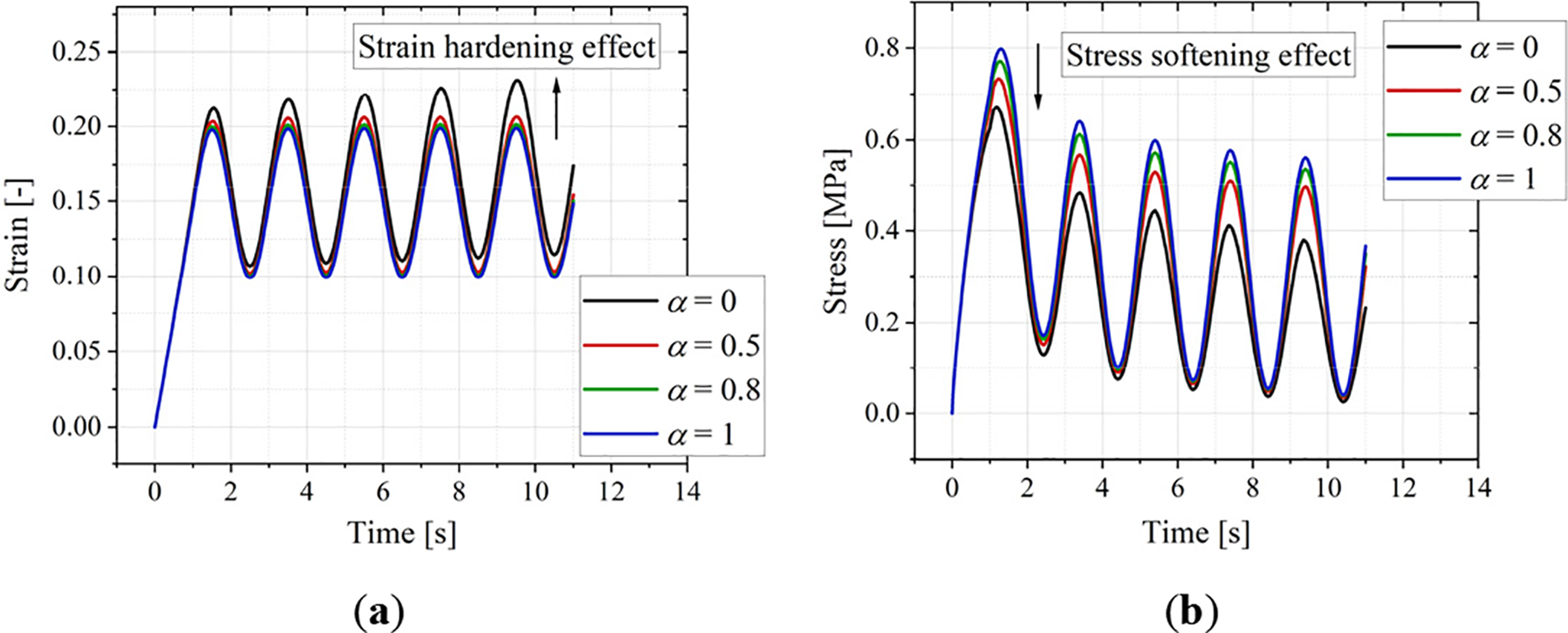
Figure 13: Cyclic loading simulation results. (a) Strain evolution over time. (b) Stress evolution over time

The influence of energy dissipation is further analyzed using the stress-strain curves depicted in Figs. 14a, 15a, and 16a. All cases exhibit a characteristic spiraling decrease in stress vs. strain, signifying the Mullins effect [57]. At α = 0 (Fig. 14a), the stress decreases markedly downward and to the right (larger spiral spacing). As α increases (Figs. 15a and 16a), the spiraling descent evolves towards a more vertical direction, with progressively smaller spiral spacing. Notably, even at α = 1 where the viscous driving energy is zero, the stress-strain curve still shows a spiraling decrease. This occurs because the inherent viscoelastic constitutive behavior (generalized Maxwell model) is still active.

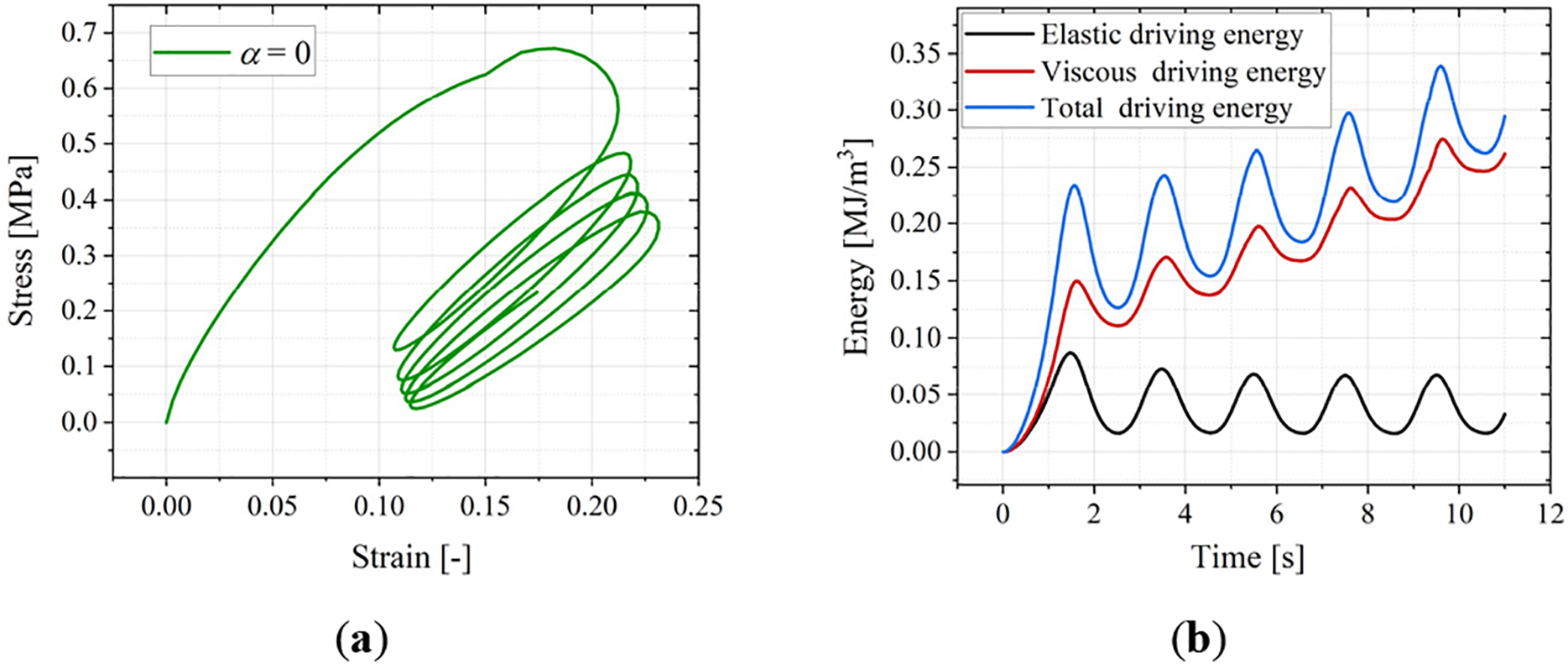
Figure 14: Cyclic loading simulation results when α = 0. (a) Stress evolution over strain. (b) Energy evolution curves

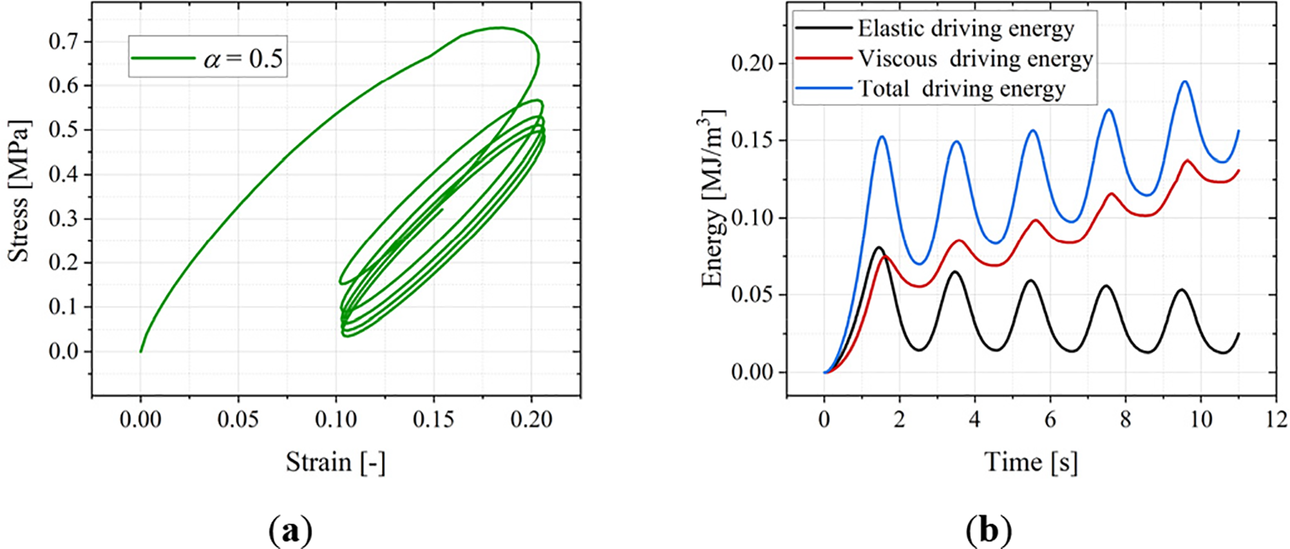
Figure 15: Cyclic loading simulation results when α = 0.5. (a) Stress evolution over strain. (b) Energy evolution curves

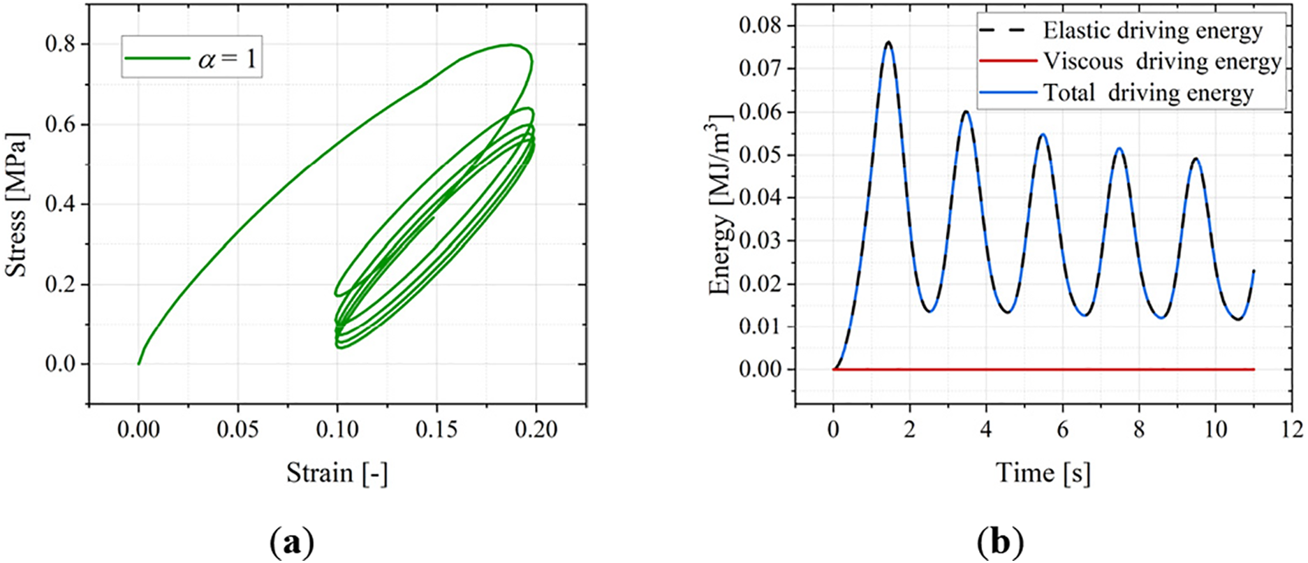
Figure 16: Cyclic loading simulation results when α = 1. (a) Stress evolution over strain. (b) Energy evolution curves

To explain this response specifically, Figs. 14b, 15b and 16b detail the evolution of the elastic driving energy, viscous driving energy, and total internal (phase-field driving) energy. These values are computed as

{ψePF=ψe0,ψvPF=αψv0,ψtPF=ψePF+ψvPF,(84)

where subscripts e, v, t correspond to elastic, viscous, and total energy, respectively.

As shown in Fig. 14b (α = 0), the amplitude of the total internal energy ψtPF steadily increases during the loading process. This increase exceeds the amplitude growth observed in Fig. 15b (α = 0.5). Consequently, at α = 0, the phase-field evolution rate is the fastest, as shown in Fig. 12b. Additionally, at α = 1 (where viscous energy is fully dissipated), the amplitude of ψtPF continually decreases, as demonstrated in Fig. 16b. This leads to the phase-field value increasing only during the first cycle and remaining constant throughout subsequent cyclic loading (Fig. 12b). This clear trend definitively confirms that viscous energy is the primary factor responsible for the stepwise and accelerated accumulation of material damage.

5.1.2 Stress Relaxation Simulation

The dogbone sample relaxation loading process lasted for a total of 1100 s. The sample is stretched to a 20% deformation within the first 100 s, and then this tensile displacement is held constant for the remaining 1000 s. Four different viscous energy dissipation conditions are considered: α = 0, α = 0.5, α = 0.8 and α = 1.

Fig. 17a shows the stress vs. time curves extracted at the reference point under different α values. It displays a typical stress relaxation process for solid propellant. It can be observed that as the α value progressively increases, the value of equilibrium stress that the material relaxes towards also becomes higher. This trend aligns with the relaxation response curves of solid propellant at different temperatures shown in Fig. 6 (where lower temperatures lead to relaxation towards a higher equilibrium tensile force). This indicates that lower temperatures reduce the viscous energy dissipation rate during material loading, making the response more elastic.

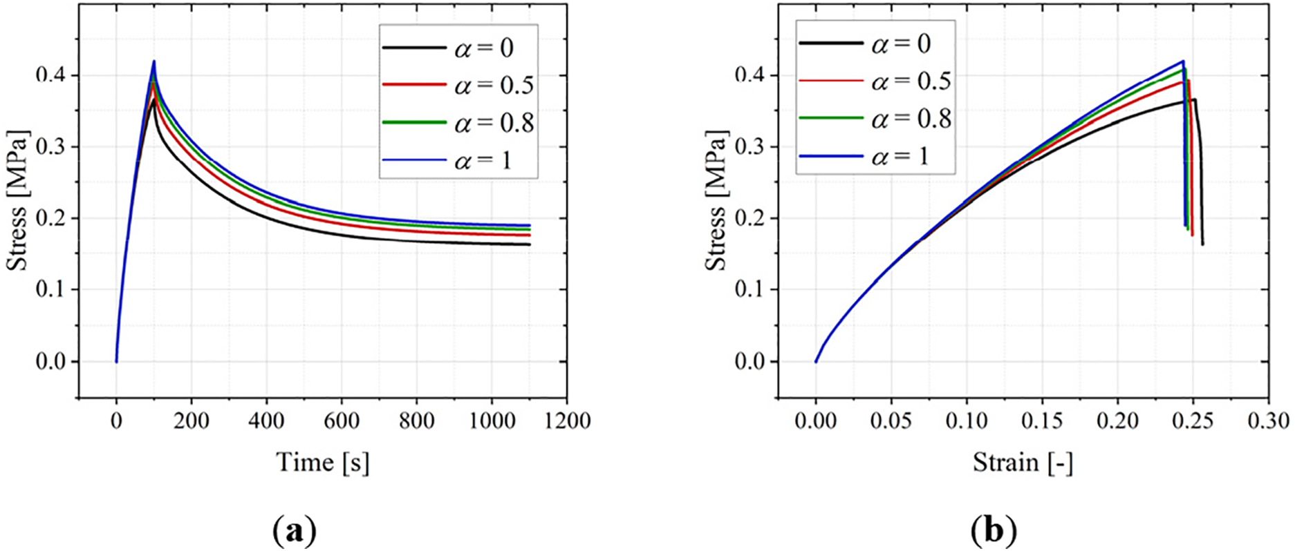
Figure 17: Stress relaxation simulation results. (a) Stress evolution over time. (b) Stress evolution over strain

Fig. 17b shows the stress-strain curves. For the curve corresponding to α = 1 (black curve), during its stress decrease phase (corresponding to the relaxation phase after 100 s in Fig. 17a), the strain continues to grow. This indicates that damage accumulation within the material did not stop during this phase.

Fig. 18a presents the evolution curves of phase-field value over time. During the tensile loading phase to 20% strain, both elastic and viscous driving energies gradually increase, leading to a rapid rise in the phase-field value for all curves. The damage accumulation rate is fastest for α = 0. During the relaxation phase (constant displacement), the phase-field values for most curves remained relatively stable. However, the curve (black one) for α = 0 showed a brief increase after 100 s.

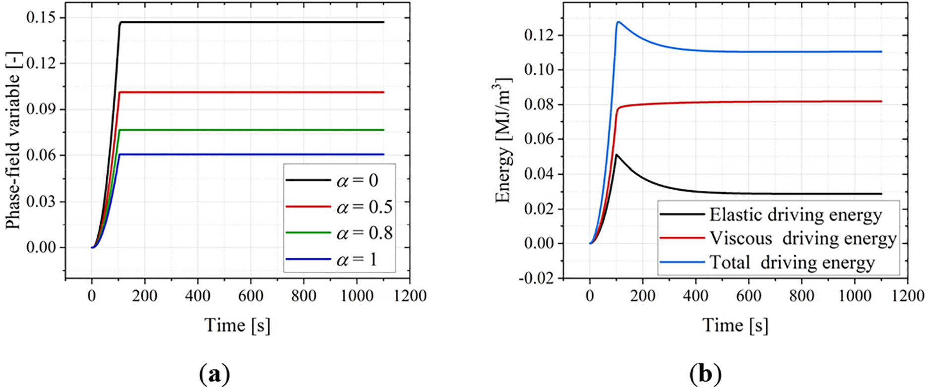
Figure 18: Stress relaxation simulation results. (a) Phase-field value evolution over time. (b) Energy evolution curves when α = 0

Fig. 18b displays the energy change curves for α = 0. During stress relaxation, the viscous energy increased while the elastic energy gradually decreased. The total phase-field driving energy decreased initially (as the rate of viscous energy increase is less than the rate of elastic energy decrease) and then slowly increased (as the rate of increase in viscous energy surpassed the rate of decrease in elastic energy). This shift underlies the continuous stress decrease observed during the relaxation phase. Fig. 19a shows the energy curves for α = 0.5, where the increase in viscous energy during relaxation is almost equal to the decrease in elastic energy. In Fig. 19b (α = 1), the increase in viscous energy is smaller than the decrease in elastic energy. Consequently, the total phase-field driving energy decreased, but the phase-field value remained constant (green curve) due to the constraint imposed by the historical energy in Eq. (27).

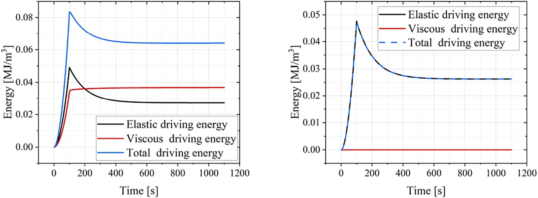
Figure 19: Stress relaxation simulation results. (a) Energy evolution curves when α = 0.5. (b) Energy evolution curves when α = 1

5.1.3 Tensile Fracture Simulation and Validation

Constant-rate tensile simulations are performed for the dogbone samples at three loading rates: 10, 100, and 500 mm/min. The model material parameters are consistent with those in Tables 1 and 2. For each loading rate, the analysis compared two scenarios representing different viscous energy dissipation proportions (α): one where α = 0.7 matched the fit value from Table 2 (where the fracture is driven by elastic and viscous energy) and another where α = 1 (where fracture is driven solely by elastic energy).

Fig. 20a shows stress-time curves revealing two key trends: (1) Tensile strength increases with loading rate, and (2) For any given rate, both maximum strength and maximum elongation increase as the viscous dissipation proportion α rises (indicating slower damage accumulation). Fig. 20b shows the corresponding evolution of the phase-field value d over time. It demonstrates that: (1) The phase-field value reaches d = 1 (complete fracture) faster under higher loading rates, signifying a reduced fracture process time; and (2) Increasing the viscous dissipation proportion α slows the rate at which d approaches 1, prolonging the fracture process.

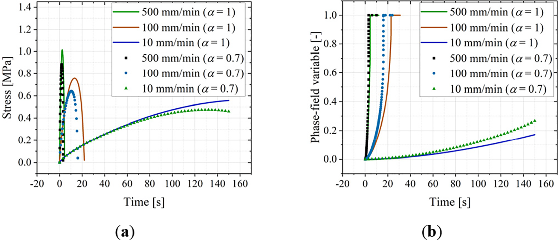
Figure 20: Tensile fracture simulation for dogbone samples: (a) Stress-time curves. (b) Phase-field value-time curves

We now validate the model’s capability to predict the mechanical response of solid propellant dogbone specimens across tensile rates of 10, 100, and 500 mm/min. In this process, the value of α is no longer fixed but is fitted and identified based on Eq. (77).

Fig. 21a–c compares the simulated and experimental force-displacement curves and present the variation in the number of iterations per increment during the tensile simulation for the three strain rates. The results demonstrate that the numerical prediction curves are in good agreement with the experimental data. Furthermore, the adaptive time-stepping scheme ensures a stable and efficient computational process—most increments converge within two or fewer iterations. Even during the stage of unstable crack propagation, the iteration count remains below two.

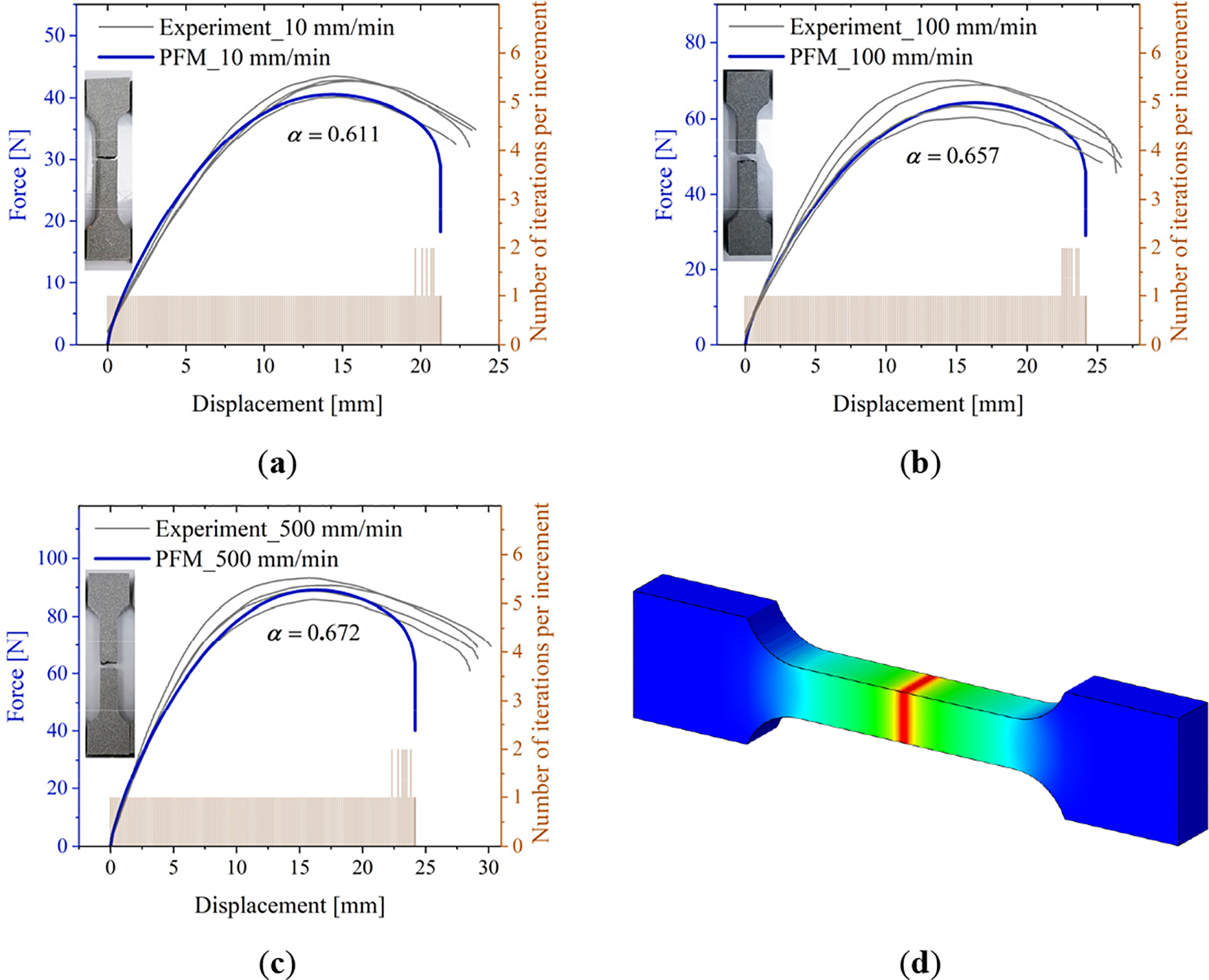
Figure 21: Numerical and experimental force-displacement responses of solid propellant specimens under different loading rates: (a) 10 mm/min, (b) 100 mm/min, (c) 500 mm/min. (d) Phase-field contour of fractured dogbone sample

Fig. 21d displays the contour plot of the tensile fracture of the dogbone specimen. Comparison with the actual fracture morphology shown in the images (depicted in Fig. 21a–c) reveals that both exhibit an opening-mode horizontal fracture. This indicates that the proposed model can accurately predict the tensile mechanical properties of solid propellant materials.

5.2 Single-Sided Notched Samples under Tensile and Shear Loading

This section details two finite element models based on the geometries of pull-off (corresponding to Mode I fracture) and shear (corresponding to Mode II fracture) specimens used in structural integrity assessment of solid rocket motor grain. The simulations focus on analyzing the crack propagation behavior of solid propellant in these two test types.

5.2.1 Mode Ⅰ Crack Propagation

The geometric dimensions and boundary conditions of the finite element model are shown in Fig. 22a. A horizontal pre-crack is set at the middle-right edge of the sample. The bottom of the sample is fixed, while a vertically upward displacement is applied to the top. The material parameters for the viscoelastic constitutive model remain consistent with those listed in Table 1. Fig. 22b shows the meshing result, consisting of 65,264 hexahedral elements. The mesh is refined in the potential crack propagation zone, with a maximum element size of h = 0.1 mm. The phase-field characteristic length is set to l0 = 4h = 0.4 mm (ensuring computational stability [23]), and the critical energy release rate is Gc = 3.8 N/mm. The study investigated three different viscous energy dissipation ratios: α = 0, α = 0.5, and α = 1.

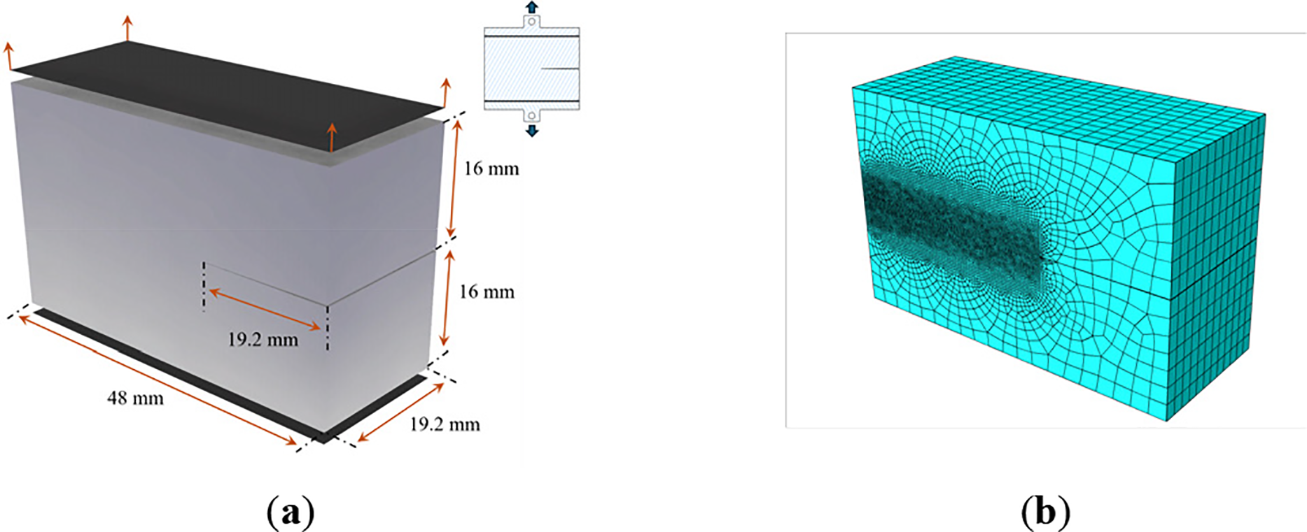
Figure 22: Model schematic of tensile test. (a) Geometric dimensions and boundary conditions. (b) Meshing

Fig. 23 presents phase-field (damage) contour plots for the calculated crack propagation under the three different α values. Under uniaxial tension, the crack propagated horizontally in all cases. Although the final crack morphology is similar across conditions, reducing the α value (increasing the viscous driving energy) significantly accelerated the crack propagation rate and expanded the material damage distribution (the damage contours for lower α show a more diffuse crack surface).

Figure 23: Phase-field fracture contours at different dissipation ratios. (a) α = 1. (b) α = 0.5. (c) α = 0

Fig. 24 shows an isosurface plot where the phase-field value d > 0.95, visually illustrating the crack morphology within the notched sample. This figure confirms that the developed phase-field framework accurately captures the crack propagation path when simulating fracture in viscoelastic materials.

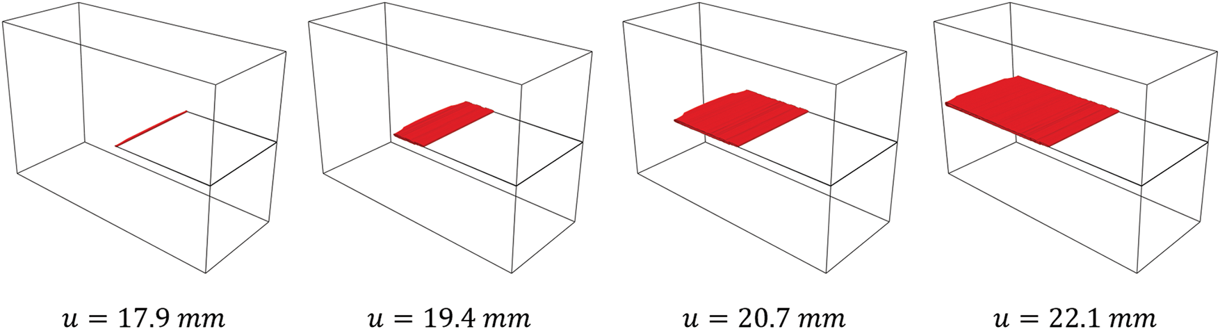
Figure 24: Isosurface (d > 0.95) of Mode I crack propagation when dissipation factor α = 0

5.2.2 Mode Ⅱ Crack Propagation

A numerical simulation of the shear response of a single-edge notched specimen is conducted to investigate the Mode II fracture. The boundary conditions and mesh discretization are illustrated in Fig. 25. To accurately capture crack propagation, a refined mesh with a maximum element size of h = 0.1 mm is employed in the potential crack propagation region. The model consists of 92,808 hexahedral elements. Simulations are also performed for three different values of the energy dissipation ratio: α = 0, α = 0.5, and α = 1. The phase-field characteristic width parameter (l0) and critical energy release rate (Gc) values remained consistent with those used in the Mode I fracture model.

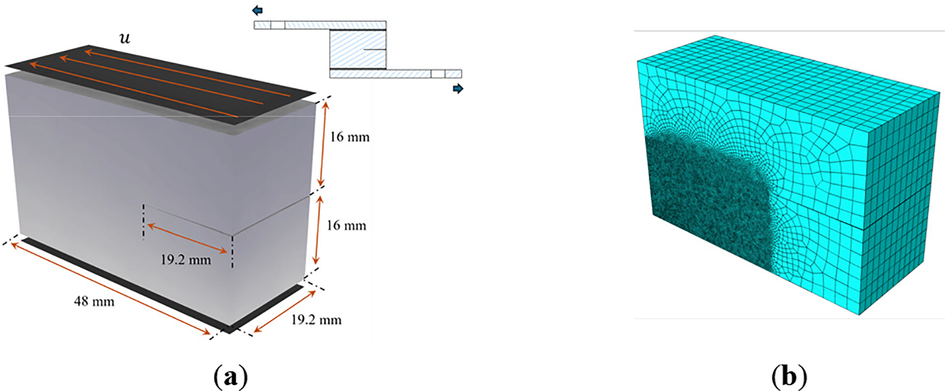
Figure 25: Calculation model schematic of shear test. (a) Geometric dimensions and boundary conditions. (b) Meshing

Fig. 26 presents the computed fracture contours (crack paths represented by the phase-field variable) under these three different dissipation ratios. The results show that under shear loading, all cracks propagated downwards and to the left. Moreover, a lower value of α led to a faster crack propagation rate.

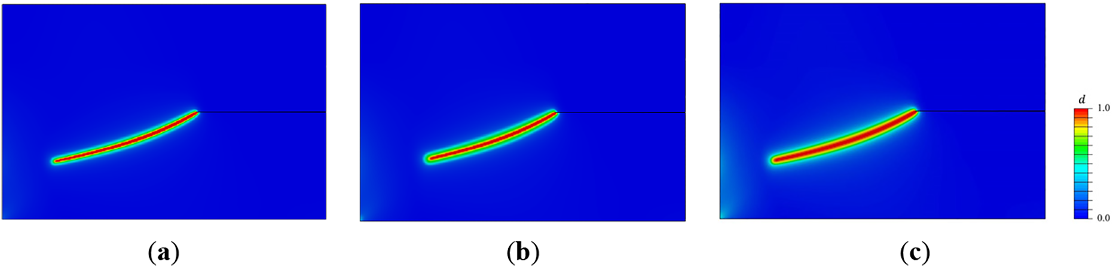
Figure 26: Phase-field fracture contours at different dissipation ratios. (a) α = 1. (b) α = 0.5. (c) α = 0

Fig. 27 further displays the 3D crack morphology corresponding to the fracture contours in Fig. 26, visualized as an isosurface where the phase-field variable d > 0.95. This figure clearly reveals the complex curved surface propagation characteristics of the current Mode II crack.

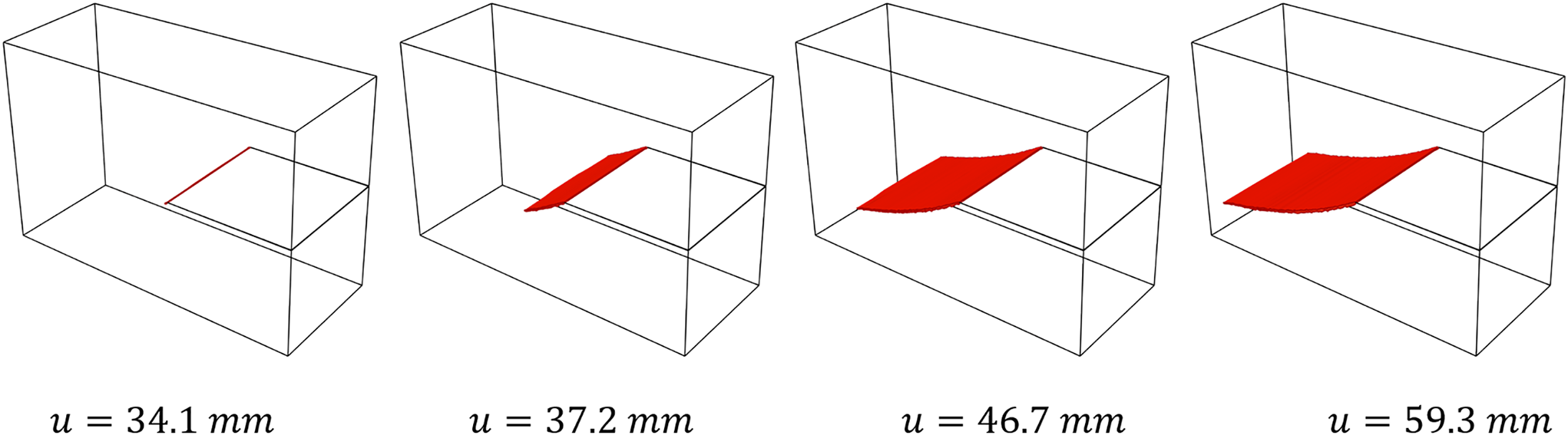
Figure 27: Isosurface (d > 0.95) of Mode Ⅱ crack propagation when dissipation factor α = 0

6  Conclusion

This study develops a viscoelastic phase-field model to characterize the fracture behavior of polymeric materials. In numerical implementation, an adaptive time-stepping iteration strategy is adopted, effectively accelerating the coupled iterative solution between the phase-field and the viscoelastic displacement field. Furthermore, all unknown parameters within the phase-field model, including the form of its degradation function, are identified by fitting experimental data. The comparative results between experiments and simulations demonstrate that the constructed model accurately predicts both the force-displacement response and the fracture morphology of solid propellants during tensile loading.

The ratio of viscous energy dissipation to storage significantly influences damage evolution in viscoelastic solids. The introduced dissipation factor α effectively quantifies the damage response of viscoelastic materials under various loading conditions, such as cyclic loading, stress relaxation, and tension. Additionally, simulations of single-edge notched specimens (representing fracture modes I and II) confirmed the model framework’s capability to accurately predict crack paths in solid propellants. Although reducing the α value accelerates crack propagation speed under identical boundary conditions, it does not alter the predicted crack path.

It should be emphasized that the proposed model assumes a zero temperature change rate (Eq. (16)) during thermodynamic derivation. This limits its direct applicability to scenarios characterized by significant thermal transients (e.g., rapid stretching or impact loading). The extension of the model to dynamic multi-axial loading scenarios necessitates further investigation. Future work will address these limitations by incorporating coupled thermo-mechanical formulations and broadening the scope of experimental validation.

Acknowledgement: Not applicable.

Funding Statement: This research is funded by National Natural Science Foundation of China (Grant No. 11872372) and Graduate Innovation Foundation of Hunan Province of China (Grant No. CX20230018).

Author Contributions: The authors confirm contribution to the paper as follows: Conceptualization, Yuan Mei and Daokui Li; methodology, Yuan Mei; software, Yuan Mei; validation, Daokui Li, Zhibin Shen and Shiming Zhou; formal analysis, Shiming Zhou; investigation, Yuan Mei; resources, Daokui Li and Shiming Zhou; data curation, Yuan Mei, Daokui Li and Shiming Zhou; writing—review and editing, Yuan Mei and Shiming Zhou; visualization, Yuan Mei; supervision, Daokui Li and Shiming Zhou; project administration, Daokui Li, Zhibin Shen and Shiming Zhou. All authors reviewed the results and approved the final version of the manuscript.

Availability of Data and Materials: The data that support the findings of this study are available from the Corresponding Author, Shiming Zhou, upon reasonable request.

Ethics Approval: Not applicable.

Conflicts of Interest: The authors declare no conflicts of interest to report regarding the present study.

References

1. Vandenkerckhove JA. Recent advances in solid propellant grain design. ARS J. 1959;29(7):483–91. doi:10.2514/8.4810. [Google Scholar] [CrossRef]

2. Wu W, Li H, Shen Z, Cui H. Research on constant speed tension and compression mechanical properties of azide polyether propellant. Propellants Explos Pyrotech. 2022;47(7):e202200055. doi:10.1002/prep.202200055. [Google Scholar] [CrossRef]

3. Movahedi-Rad AV, Keller T, Vassilopoulos AP. Modeling of fatigue behavior based on interaction between time- and cyclic-dependent mechanical properties. Compos Part A Appl Sci Manuf. 2019;124:105469. doi:10.1016/j.compositesa.2019.05.037. [Google Scholar] [CrossRef]

4. Adel WM, Liang G. Service life prediction of AP/Al/HTPB solid rocket propellant with consideration of softening aging behavior. Chin J Aeronaut. 2019;32(2):361–8. doi:10.1016/j.cja.2018.08.003. [Google Scholar] [CrossRef]

5. Sun Q, Zhou G, Meng Z, Guo H, Chen Z, Liu H, et al. Failure criteria of unidirectional carbon fiber reinforced polymer composites informed by a computational micromechanics model. Compos Sci Technol. 2019;172:81–95. doi:10.1016/j.compscitech.2019.01.012. [Google Scholar] [CrossRef]

6. Greenhalgh E. Failure analysis and fractography of polymer composites. New York, NY, USA: Elsevier; 2009. [Google Scholar]

7. Wang ZJ, Qiang HF. Mechanical properties of thermal aged HTPB composite solid propellant under confining pressure. Def Technol. 2022;18(4):618–25. doi:10.1016/j.dt.2021.06.014. [Google Scholar] [CrossRef]

8. Labuz JF, Zang A. Mohr-coulomb failure criterion. Rock Mech Rock Eng. 2012;45(6):975–9. doi:10.1007/s00603-012-0281-7. [Google Scholar] [CrossRef]

9. Li M, Li Z, He H, Chen L, Miao Y. Mechanical behaviors and constitutive relations under wide strain rate range for CMDB propellant. Polym Test. 2022;116:107806. doi:10.1016/j.polymertesting.2022.107806. [Google Scholar] [CrossRef]

10. Wang J, Cheng J, Lei M, Hu X, Wen L. Mechanical properties and constitutive model of a composite solid propellant under the synergistic effects of accelerated aging time, pre-strain, and damage growth. Mech Mater. 2020;148:103453. doi:10.1016/j.mechmat.2020.103453. [Google Scholar] [CrossRef]

11. Li H, Xu J, Jin F, Li P, Fan Z. Structural integrity assessment of a solid propellant grain considering confining pressure effect. Int J Press Vessel Pip. 2024;211:105272. doi:10.1016/j.ijpvp.2024.105272. [Google Scholar] [CrossRef]

12. Valverde-González A, Martínez-Pañeda E, Quintanas-Corominas A, Reinoso J, Paggi M. Computational modelling of hydrogen assisted fracture in polycrystalline materials. Int J Hydrogen Energy. 2022;47(75):32235–51. doi:10.1016/j.ijhydene.2022.07.117. [Google Scholar] [CrossRef]

13. Nguyen-Thanh N, Li W, Huang J, Zhou K. Adaptive higher-order phase-field modeling of anisotropic brittle fracture in 3D polycrystalline materials. Comput Methods Appl Mech Eng. 2020;372:113434. doi:10.1016/j.cma.2020.113434. [Google Scholar] [CrossRef]

14. Khokhlov N, Stognii P. Novel approach to modeling the seismic waves in the areas with complex fractured geological structures. Minerals. 2020;10(2):122. doi:10.3390/min10020122. [Google Scholar] [CrossRef]

15. Tang J, Wang X, Du X, Ma B, Zhang F. Optimization of integrated geological-engineering design of volume fracturing with fan-shaped well pattern. Pet Explor Dev. 2023;50(4):971–8. doi:10.1016/S1876-3804(23)60442-2. [Google Scholar] [CrossRef]

16. Zhang P, Wang C, Gao Z, Wang F. A review on fracture properties of steel fiber reinforced concrete. J Build Eng. 2023;67:105975. doi:10.1016/j.jobe.2023.105975. [Google Scholar] [CrossRef]

17. Chang Z, Zhang H, Schlangen E, Šavija B. Lattice fracture model for concrete fracture revisited: calibration and validation. Appl Sci. 2020;10(14):4822. doi:10.3390/app10144822. [Google Scholar] [CrossRef]

18. Aravind R, Natarajan S, Jayakumar K, Annabattula RK. A non-intrusive stochastic phase-field for fatigue fracture in brittle materials with uncertainty in geometry and material properties. Comput Model Eng Sci. 2024;141(2):997–1032. doi:10.32604/cmes.2024.053047. [Google Scholar] [CrossRef]

19. Quinteros L, García-Macías E, Martínez-Pañeda E. Electromechanical phase-field fracture modelling of piezoresistive CNT-based composites. Comput Methods Appl Mech Eng. 2023;407:115941. doi:10.1016/j.cma.2023.115941. [Google Scholar] [CrossRef]

20. Navidtehrani Y, Betegón C, Martínez-Pañeda E. A general framework for decomposing the phase field fracture driving force, particularised to a Drucker-Prager failure surface. Theor Appl Fract Mech. 2022;121:103555. doi:10.1016/j.tafmec.2022.103555. [Google Scholar] [CrossRef]

21. Bui TQ, Hu X. A review of phase-field models, fundamentals and their applications to composite laminates. Eng Fract Mech. 2021;248:107705. doi:10.1016/j.engfracmech.2021.107705. [Google Scholar] [CrossRef]

22. Dammaß F, Ambati M, Kästner M. Phase-field modelling and simulation of fracture in viscoelastic materials. PAMM. 2021;21(1):e202100108. doi:10.1002/pamm.202100108. [Google Scholar] [CrossRef]

23. Yuan H, Tang W, He J, Guan X. An efficient phase-field model for fatigue fracture in viscoelastic solids using cyclic load decomposition and damage superposition. Comput Methods Appl Mech Eng. 2024;418:116469. doi:10.1016/j.cma.2023.116469. [Google Scholar] [CrossRef]

24. Marulli MR, Valverde-González A, Quintanas-Corominas A, Paggi M, Reinoso J. A combined phase-field and cohesive zone model approach for crack propagation in layered structures made of nonlinear rubber-like materials. Comput Methods Appl Mech Eng. 2022;395:115007. doi:10.1016/j.cma.2022.115007. [Google Scholar] [CrossRef]

25. Miehe C, Schänzel LM. Phase field modeling of fracture in rubbery polymers. Part I: finite elasticity coupled with brittle failure. J Mech Phys Solids. 2014;65:93–113. doi:10.1016/j.jmps.2013.06.007. [Google Scholar] [CrossRef]

26. Liu Z, Roggel J, Juhre D. Phase-field modelling of fracture in viscoelastic solids. Procedia Struct Integr. 2018;13:781–6. doi:10.1016/j.prostr.2018.12.129. [Google Scholar] [CrossRef]

27. Shen R, Waisman H, Guo L. Fracture of viscoelastic solids modeled with a modified phase field method. Comput Methods Appl Mech Eng. 2019;346:862–90. doi:10.1016/j.cma.2018.09.018. [Google Scholar] [CrossRef]

28. Dammaß F, Ambati M, Kästner M. A unified phase-field model of fracture in viscoelastic materials. Contin Mech Thermodyn. 2021;33(4):1907–29. doi:10.1007/s00161-021-01013-3. [Google Scholar] [CrossRef]

29. Yuan H, Guan X. Phase-field viscoelastic fracture modeling of polymer composites using strain tensor spectral decomposition. Comput Methods Appl Mech Eng. 2023;410:116018. doi:10.1016/j.cma.2023.116018. [Google Scholar] [CrossRef]

30. Heinrich G, Kipscholl R, Le Cam JB, Stoček R. Advances in understanding thermal effects in rubber: experiments, modelling, and practical relevance. Cham, Switzerland: Springer; 2024. p. 95–123. doi:10.1007/978-3-031-71056-8. [Google Scholar] [CrossRef]

31. Choo J, Sun W. Coupled phase-field and plasticity modeling of geological materials: from brittle fracture to ductile flow. Comput Methods Appl Mech Eng. 2018;330:1–32. doi:10.1016/j.cma.2017.10.009. [Google Scholar] [CrossRef]

32. Miehe C, Hofacker M, Welschinger F. A phase field model for rate-independent crack propagation: robust algorithmic implementation based on operator splits. Comput Methods Appl Mech Eng. 2010;199(45–48):2765–78. doi:10.1016/j.cma.2010.04.011. [Google Scholar] [CrossRef]

33. Xia X, Qin C, Lu G, Gu X, Zhang Q. Simulation of corrosion-induced cracking of reinforced concrete based on fracture phase field method. Comput Model Eng Sci. 2024;138(3):2257–76. doi:10.32604/cmes.2023.031238. [Google Scholar] [CrossRef]

34. Hu X, Zhang P, Yao W. Phase field modelling of microscopic failure in composite laminates. J Compos Mater. 2021;55(14):1853–65. doi:10.1177/0021998320976794. [Google Scholar] [CrossRef]

35. Loew PJ, Peters B, Beex LAA. Rate-dependent phase-field damage modeling of rubber and its experimental parameter identification. J Mech Phys Solids. 2019;127:266–94. doi:10.1016/j.jmps.2019.03.022. [Google Scholar] [CrossRef]

36. Tanné E, Li T, Bourdin B, Marigo JJ, Maurini C. Crack nucleation in variational phase-field models of brittle fracture. J Mech Phys Solids. 2018;110:80–99. doi:10.1016/j.jmps.2017.09.006. [Google Scholar] [CrossRef]

37. Miehe C, Welschinger F, Hofacker M. Thermodynamically consistent phase-field models of fracture: variational principles and multi-field FE implementations. Int J Numer Methods Eng. 2010;83(10):1273–311. doi:10.1002/nme.2861. [Google Scholar] [CrossRef]

38. Francfort GA, Marigo JJ. Revisiting brittle fracture as an energy minimization problem. J Mech Phys Solids. 1998;46(8):1319–42. doi:10.1016/S0022-5096(98)00034-9. [Google Scholar] [CrossRef]

39. Bourdin B, Francfort GA, Marigo JJ. Numerical experiments in revisited brittle fracture. J Mech Phys Solids. 2000;48(4):797–826. doi:10.1016/S0022-5096(99)00028-9. [Google Scholar] [CrossRef]

40. Wu JY. A unified phase-field theory for the mechanics of damage and quasi-brittle failure. J Mech Phys Solids. 2017;103:72–99. doi:10.1016/j.jmps.2017.03.015. [Google Scholar] [CrossRef]

41. Gültekin O, Dal H, Holzapfel GA. A phase-field approach to model fracture of arterial walls: theory and finite element analysis. Comput Methods Appl Mech Eng. 2016;312:542–66. doi:10.1016/j.cma.2016.04.007. [Google Scholar] [PubMed] [CrossRef]

42. Loew PJ, Poh LH, Peters B, Beex LAA. Accelerating fatigue simulations of a phase-field damage model for rubber. Comput Methods Appl Mech Eng. 2020;370:113247. doi:10.1016/j.cma.2020.113247. [Google Scholar] [CrossRef]

43. Klinsmann M, Rosato D, Kamlah M, McMeeking RM. An assessment of the phase field formulation for crack growth. Comput Methods Appl Mech Eng. 2015;294:313–30. doi:10.1016/j.cma.2015.06.009. [Google Scholar] [CrossRef]

44. Borden MJ, Hughes TJR, Landis CM, Anvari A, Lee IJ. A phase-field formulation for fracture in ductile materials: finite deformation balance law derivation, plastic degradation, and stress triaxiality effects. Comput Methods Appl Mech Eng. 2016;312:130–66. doi:10.1016/j.cma.2016.09.005. [Google Scholar] [CrossRef]

45. de Borst R, Verhoosel CV. Gradient damage vs phase-field approaches for fracture: similarities and differences. Comput Methods Appl Mech Eng. 2016;312:78–94. doi:10.1016/j.cma.2016.05.015. [Google Scholar] [CrossRef]

46. Wu JY, Nguyen VP. A length scale insensitive phase-field damage model for brittle fracture. J Mech Phys Solids. 2018;119:20–42. doi:10.1016/j.jmps.2018.06.006. [Google Scholar] [CrossRef]

47. Singh N, Verhoosel CV, de Borst R, van Brummelen EH. A fracture-controlled path-following technique for phase-field modeling of brittle fracture. Finite Elem Anal Des. 2016;113:14–29. doi:10.1016/j.finel.2015.12.005. [Google Scholar] [CrossRef]

48. Adams RA, Fournier JJF. Sobolev spaces. New York, NY, USA: Elsevier; 2003. [Google Scholar]

49. Ambati M, Gerasimov T, De Lorenzis L. A review on phase-field models of brittle fracture and a new fast hybrid formulation. Comput Mech. 2015;55(2):383–405. doi:10.1007/s00466-014-1109-y. [Google Scholar] [CrossRef]

50. Abaqus G. Abaqus 6.11. Providence, RI, USA: Dassault Systemes Simulia Corporation; 2011. [Google Scholar]

51. Miehe C, Kienle D, Aldakheel F, Teichtmeister S. Phase field modeling of fracture in porous plasticity: a variational gradient-extended Eulerian framework for the macroscopic analysis of ductile failure. Comput Methods Appl Mech Eng. 2016;312:3–50. doi:10.1016/j.cma.2016.09.028. [Google Scholar] [CrossRef]

52. Hufferd W, Fitzgerald J. JANNAF solid propellant structural integrity handbook. Laurel, MD, USA: Chemical Propulsion Information Agency; 1987. [Google Scholar]

53. ASTM D. Standard test method for tensile properties of plastics. West Conshohocken, PA, USA: ASTM International; 2014. [Google Scholar]

54. Mei Y, Li DK, Zhou SM, Shen ZB, Wu WJ. Identification of viscoelastic parameters for composite propellant by indentation technique. Propellants Explos Pyrotech. 2023;48(3):e202200309. doi:10.1002/prep.202200309. [Google Scholar] [CrossRef]

55. Sargado JM, Keilegavlen E, Berre I, Nordbotten JM. High-accuracy phase-field models for brittle fracture based on a new family of degradation functions. J Mech Phys Solids. 2018;111:458–89. doi:10.1016/j.jmps.2017.10.015. [Google Scholar] [CrossRef]

56. Kuhn C, Schlüter A, Müller R. On degradation functions in phase field fracture models. Comput Mater Sci. 2015;108:374–84. doi:10.1016/j.commatsci.2015.05.034. [Google Scholar] [CrossRef]

57. Mullins L. Softening of rubber by deformation. Rubber Chem Technol. 1969;42(1):339–62. doi:10.5254/1.3539210. [Google Scholar] [CrossRef]