
 Submit a Paper
 Propose a Special lssue
 Open Access
ARTICLE

Numerical Analysis of Heat and Mass Transfer in Tangent Hyperbolic Fluids Using a Two-Stage Exponential Integrator with Compact Spatial Discretization
1 Department of Mathematics, COMSATS University Islamabad, Park Road, Islamabad, 45550, Pakistan
2 Department of Mathematics and Sciences, College of Science and Humanities, Prince Sultan University, Riyadh, 11586, Saudi Arabia
3 Department of Mathematics, Faculty of Engineering and Computing, National University of Modern Languages (NUML), Islamabad, 44000, Pakistan
4 Department of Mathematics and Statistics, College of Science, Imam Mohammad Ibn Saud Islamic University (IMSIU), P.O. Box 90950, Riyadh, 11623, Saudi Arabia
* Corresponding Author: Nabil Kerdid. Email:
Computer Modeling in Engineering & Sciences 2025, 145(1), 537-569. https://doi.org/10.32604/cmes.2025.070362
Received 14 July 2025; Accepted 17 September 2025; Issue published 30 October 2025
 View Full Text
 Download PDF
Abstract
This study develops a high-order computational scheme for analyzing unsteady tangent hyperbolic fluid flow with variable thermal conductivity, thermal radiation, and coupled heat and mass transfer effects. A modified two-stage Exponential Time Integrator is introduced for temporal discretization, providing second-order accuracy in time. A compact finite difference method is employed for spatial discretization, yielding sixth-order accuracy at most grid points. The proposed framework ensures numerical stability and convergence when solving stiff, nonlinear parabolic systems arising in fluid flow and heat transfer problems. The novelty of the work lies in combining exponential integrator schemes with compact high-order spatial discretization, enabling accurate and efficient simulations of tangent hyperbolic fluids under complex boundary conditions, such as oscillatory plates and varying thermal conductivity. This approach addresses limitations of classical Euler, Runge–Kutta, and spectral methods by significantly reducing numerical errors (up to 45%) and computational cost. Comprehensive parametric studies demonstrate how viscous dissipation, chemical reactions, the Weissenberg number, and the Hartmann number influence flow behaviour, heat transfer, and mass transfer. Notably, heat transfer rates increase by 18.6% with stronger viscous dissipation, while mass transfer rates rise by 21.3% with more intense chemical reactions. The real-world relevance of the study is underscored by its direct applications in polymer processing, heat exchanger design, radiative thermal management in aerospace, and biofluid transport in biomedical systems. The proposed scheme thus provides a robust numerical framework that not only advances the mathematical modelling of non-Newtonian fluid flows but also offers practical insights for engineering systems involving tangent hyperbolic fluids.Keywords
Non-Newtonian fluids are characterized by variable viscosity, meaning that a constant viscosity does not govern their flow properties. Instead, the viscosity of these fluids can alter in response to the applied stress or strain rate. From these options, the tangent-hyperbolic fluids are interesting in how completely they can describe a general phenomenon, namely, that of shear-thinning, which is observed in all kinds of industrial and biological Fluids [1]. They are, therefore, of great significance in many applications, ranging from food processing to biomedical engineering. Under different thermodynamic conditions and varying circumstances, understanding their behaviour is one of the key steps in enhancing these values in practical applications.
Classical finite difference and finite volume methods have been widely used for discretizing the governing equations. These methods are straightforward to implement, but tend to exhibit lower accuracy and stability issues for stiff or highly nonlinear problems. To improve temporal resolution, Runge–Kutta (RK) and predictor–corrector methods have been introduced, offering better stability control. However, the conventional RK methods can become computationally expensive and may still struggle with systems exhibiting rapid oscillations or sharp gradients, especially in coupled thermofluid problems. Another prominent family of approaches is the nonstandard finite difference (NSFD) scheme, which is constructed to preserve important qualitative properties, such as positivity, boundedness, and stability. While they offer structural advantages in some biological and epidemiological models, their accuracy and adaptability are generally limited in multi-dimensional transport scenarios with complex boundary conditions.
Exponential Time Integrator methods have recently gained traction as an effective solution strategy for stiff systems. These methods treat the linear part of the PDE exactly via matrix exponentials, while nonlinear terms are handled through various approximations. They are particularly suitable for flows with oscillatory or wave-like behaviour, where traditional methods may either require small time steps or fail to capture the transient features accurately.
Any fluid that deviates from Newton’s Law of Viscosity is called a non-Newtonian fluid. It is common for the viscosities of non-Newtonian fluids to be determined by the shear rate or its history. Nonetheless, normal stress differences or non-Newtonian behaviour can be observed in certain non-Newtonian fluids with shear-independent viscosity. Commonplace items like ketchup, custard, toothpaste, starch suspensions, paint, blood, and shampoo are among the numerous commonly found compounds that exhibit non-Newtonian fluid behaviour. Molten polymers and salt solutions are also examples of this. The viscosity coefficient is the proportionality constant in the linear relationship between shear stress and shear rate in a Newtonian fluid, which passes through the origin [2].
The magnetohydrodynamic (MHD) peristaltic flow of a fluid model in an asymmetrical vertical channel was studied by Nadeem and Akram [3] using the hyperbolic tangent function. The length of the flow’s wavelength was assumed to be considerable. Utilizing the finite difference Keller box method, Gaffar et al. [4] investigated the heat transfer and flow of a non-Newtonian tangent hyperbolic fluid emanating from a sphere. The investigation focused on the nonlinear boundary layer behaviour of the incompressible fluid. Non-Newtonian tangent hyperbolic fluid flow with heat radiation in the presence of a cylinder is the subject of Gnaneswara Reddy et al.’s [5] magnetohydrodynamic investigation. In this work, we use the sheet velocity distribution suggested by Xu and Liao [6] to analyze the power-law non-Newtonian fluids’ laminar flow and heat transfer properties across a stretching sheet. In a study conducted by Megahed [7], the effects of thermal radiation, heat buoyancy, and non-Newtonian power-law fluid flow were investigated across a non-linearly vertical surface. The effects of viscous dissipation and heat source were considered in the study of fluid flow and heat transmission over a stretching sheet by Gnaneswara Reddy et al. [8]. In their work, Choudhary et al. [9] examine how a thick and incompressible fluid behaves as it moves across a stretched surface. Either fluid can travel through the surface or be suctioned or injected through it.
The tangent hyperbolic fluid model can accurately define the shear-thinning process. The measurement involves determining the decrease in fluid flow rate due to increased shear stress. Several literature reports have analyzed the tangent hyperbolic fluid, examining its numerous physical characteristics. The convective heat transport of a non-Newtonian tangent hyperbolic fluid was studied by Hussain et al. [10]. A nonlinear stretching sheet was the primary object of their attention as they studied the consequences of viscous dissipation. The analysis employed the HAM (Homotopy Analysis Method) and shooting technique. Partha et al. [11] investigated the phenomenon of mixed convective flow and heat transmission from a surface that is exponentially stretching while considering the effect of viscous dissipation. Considering thermal dispersion, the study examines the mass and heat transfer in a two-dimensional magnetohydrodynamic (MHD) boundary layer flow involving a tangent hyperbolic fluid. According to the findings of Uma and Koteswara, the four-constant fluid model, known as the electrically conducting tangent hyperbolic fluid, may adequately depict the effects of shear thinning [12]. Under an exponentially decreasing heat source, Mamatha et al. [13] studied the behaviour of an incompressible magnetohydrodynamic (MHD) Carreau Dusty fluid moving across a stretching sheet. Non-Newtonian fluids with hyperbolic tangent behavior and subjected to a magnetic field on a vertical permeable cone were studied by Gaffar et al. [14] in terms of flow and heat transfer. This study mainly aimed to understand non-isothermal steady-state boundary layer conditions. Researchers Raju et al. [15] examined the magnetohydrodynamic (MHD) Casson fluid’s flow, heat, and mass transport characteristics across an exponentially expanding surface. A comparison of the Casson fluid’s results with those of a Newtonian fluid revealed two distinct solutions. Dessie and Kishan [16] investigated a viscous porosity-flowing fluid and heat transmission over a stretched sheet. Specifically, they looked at the interactions between a heat source and sink, a magnetic field, and viscous dissipation. The flow and heat transfer characteristics of a non-Newtonian hyperbolic tangent fluid were investigated by Naseer et al. [17] using an exponentially stretched, vertically oriented cylinder.
The primary challenge in computational fluid dynamics (CFD) is numerically integrating partial differential equations (PDEs) that are subject to time-evolving conditions. Various time integrators may be applied following the problems’ specific requirements, from simple direct methods to complex implicit schemes. It should be noted that although explicit systems are easy to set up, they can produce results of dubious accuracy, particularly when solving stiff equations. Conversely, implicit techniques typically require solving large sets of algebraic equations at each time step, resulting in a significant increase in calculation time.
An exponential integrator could solve stiff PDEs. They utilize exponential functions to overcome stiffness more effectively than standard methods [18]. Two-stage exponential integrators are used to solve parabolic partial differential equations, such as those in fluid dynamics, because they are efficient and modest. When calculating heat transfer in the presence of a non-uniform heat source or sink, Abel et al. [19] took into account the power-law fluid’s flow as a consequence of a linear stretching sheet. In a symmetrically inclined channel, the peristaltic flow of a hyperbolic tangent fluid through a porous medium is studied at low Reynolds numbers and long wavelengths, as stated by Jyothi et al. [20]. The dynamics of nanofluid boundary layer flow over a stretching surface were studied by Vendabai [21], who considered the variable radiation impact resulting from the presence of the heat source. An unstable flow of a nanofluid across a stretching sheet with a convective boundary condition is considered by Mansur and Ishak [22] in terms of its heat transfer properties. In their study, Sarojamma and Vendabai [23] investigated the impact of a transverse magnetic field and a heat source on the boundary layer flow of a Casson nanofluid over an exponentially expanding cylinder.
Non-Newtonian fluids that obey a rheological equation within a narrow range are called tangent hyperbolic fluids. This range ensures that the fluid maintains its shear-thinning nature. The equation is valid when the time-dependent material
A lot of progress has been achieved in the last several years in the numerical simulation of non-Newtonian fluid flows with thermal and magnetic effects, notably for power-law and tangent hyperbolic models. Arif et al. [28] developed a hybrid computational framework for the analysis of electro-osmotic flow in Carreau fluids, providing improved accuracy in microchannel applications. Nawaz et al. [29] put forward a compact high-order approach for simulating viscous dissipation in MHD boundary layer flow, which demonstrated enhanced resolution of steep gradients next to boundaries. Researchers have also looked at more advanced data-driven methods. For example, Shoaib et al. [30] used stochastic neural networks to study Maxwell nanofluids under MHD effects with promising accuracy. Ullah et al. [31] utilized Levenberg Marquardt algorithms for micropolar flow with mass injection in porous media, demonstrating the capabilities of AI-assisted solvers. Additionally, Rehman et al. [32] performed a neural network-based examination of Williamson fluid flow in thermally sliding magnetic fields, which roughly corresponds with the objectives of the current study. These results indicate a transition towards compact, adaptive, and data-driven numerical techniques, hence confirming our initiative to present a specific exponential integrator scheme with compact spatial discretization for tangent hyperbolic fluid flows.
Research Gap: Although significant progress has been made in modelling non-Newtonian fluid dynamics, most existing studies still focus on simplified flow configurations, neglecting the combined influence of magnetic fields, porous media resistance, oscillatory boundary conditions, and complex shear-thinning rheology. Furthermore, electro-osmotic and thermal effects are often investigated in isolation, limiting the ability to capture realistic multi-physics interactions. Another limitation lies in the numerical strategies typically employed: conventional first- and second-order schemes frequently encounter challenges in stability and accuracy when applied to highly coupled transport problems. This creates a clear research gap in developing computationally efficient, high-order numerical frameworks that can simultaneously account for velocity, temperature, and concentration fields in porous, electrically active environments under the influence of magnetic forces and thermal gradients. To address this gap, the present study introduces a compact finite difference–based two-stage exponential integrator specifically designed to simulate tangent hyperbolic fluids with inclined magnetic fields, viscous dissipation, and chemical reaction phenomena. Comparative analysis shows that the proposed scheme reduces the
Contributions and Significance: The primary objective of this project is to create and implement an improved numerical method, known as the modified Exponential Time Integrator, for the precise simulation of the flow of tangent hyperbolic fluids with varying thermal conductivity. This entails measuring and analyzing the impact of viscous dissipation and chemical reactions in dynamic situations. By examining the unsteady flow across moving plates, this study aims to gain a deeper understanding of the complex relationships between fluid characteristics, external forces, and thermal fluctuations. In conclusion, this research expands our understanding of non-Newtonian fluid dynamics and offers practical solutions for engineering applications that involve these fluids.
This work employs a numerical technique to solve time-dependent partial differential equations. The scheme is formulated via a Taylor series expansion, incorporating an existing first-order time integrator alongside a novel second stage, referred to as the corrected scheme. To discretize spatial coordinates, the compact difference scheme is employed. The compact scheme can provide fourth-or sixth-order accuracy in space. The scheme addresses the problem of boundary layer flow over the flat and oscillatory plate. The non-Newtonian and incompressible fluid is considered. Despite converting governing equations into ordinary differential equations, the transformations that convert the dimensional governing equations into a dimensionless set of partial differential equations are employed. A set of partial differential equations is solved using the proposed approach, which achieves second-order accuracy in time and sixth-order accuracy in space at most grid points. This research advances the discipline by:
1. Unlike earlier studies that primarily relied on classical explicit or implicit integrators (e.g., the Keller-Box method, the shooting method, and the Runge–Kutta method), we develop a two-stage compact exponential time integrator method. This method delivers second-order temporal accuracy and sixth-order spatial accuracy, which significantly improves both efficiency and accuracy for stiff parabolic PDEs compared to standard second-order schemes.
2. While many prior works focused only on either magnetic effects, porous media, or thermal radiation individually, our study considers the combined influence of thermal radiation, variable thermal conductivity, viscous dissipation, and chemical reactions on tangent hyperbolic fluids. This comprehensive framework is not reported in earlier literature.
3. Through rigorous numerical experiments, we demonstrate that the proposed scheme achieves up to 45% error reduction compared to conventional approaches, thereby showing a substantial methodological improvement that enhances stability and convergence.
4. The proposed framework is tailored for real-world applications, including magnetohydrodynamic flows in porous structures, electrokinetic biofluid transport, and radiative cooling in thermal systems. Unlike previous studies with simplified geometries, we incorporate oscillatory boundary conditions and multi-parameter interactions, making the model directly applicable to biomedical, polymer, and petroleum engineering processes.
Quantitative Results: This work proposes a compact two-stage exponential method that enhances solution accuracy while handling the nonlinearities associated with tangent hyperbolic fluids. The method shows a reduction in numerical error by up to 45% compared to standard second-order schemes. Parametric studies indicate a notable enhancement of 18.6% in heat transfer rates due to viscous dissipation effects, which increase the Eckert number, and a 21.3% increase in mass transfer rate, resulting from stronger chemical reactions. These findings validate the significance of the proposed method in practical applications involving heat exchangers, polymer processing, and biomedical flows.
The real-world relevance of this study:
The direct application of the mathematical framework and computational scheme developed in this work to industrial processes involving magnetohydrodynamic (MHD) flows in porous channels is possible, including polymer extrusion, thermal management in microelectronic systems, radiative cooling in aerospace structures, and biofluid dynamics involving electrokinetic transport. In biomedical engineering, they help create targeted drug administration systems under oscillatory flow conditions. In petroleum engineering, such models are essential for simulating enhanced oil recovery technologies that employ magnetic nanoparticles.
The subsequent sections of this document are organized as follows: Section 2 provides a comprehensive explanation of the creation of the two-stage exponential integrator and a concise spatial discretization scheme. Sections 3 and 4 present the stability and convergence study of the suggested approach. Section 5 examines the implementation and application of the scheme for the flow of tangent hyperbolic fluid over flat and oscillatory sheets. Section 6 evaluates the efficacy of the proposed strategy by comparing it to existing numerical methods. Section 7 concludes the work by providing a concise overview of the findings and suggesting potential avenues for future research.
2 Proposed Exponential Time Integrator Scheme
The proposed scheme can be referred to as an exponential time integrator because it integrates the time-dependent term in the convection-diffusion problem. The first stage of the scheme is first-order accurate and can also be referred to as a predictor scheme. The second stage of the scheme is corrector one, and both stages provide second-order accuracy in time. To propose a scheme, consider the following equation.
Eq. (1) models many real systems, such as heat transfer in blood vessels (non-Newtonian tangent hyperbolic fluid), pollutant transport in a fluid near an oscillating plate, and thermal diffusion in thin films on vibrating substrates. It includes
Subject to initial and boundary conditions
where
2.1 Rewriting the PDE as Exponential-Friendly Form
Before starting the construction procedure of the scheme, Eq. (1) can be written as
where
2.2 First Stage Predictor (First-Order Exponential Step)
Now, the first stage of the scheme is expressed as
where
2.3 Second Stage Corrector (Full Scheme with 2nd Order Accuracy)
The second stage of the scheme consists of two parameters, which will be determined by matching the coefficients of the Taylor series expansion. Here, we use both current
Expanding
By using Eqs. (5) and (7) into Eq. (6), it is obtained
By equating the coefficients of
By solving Eq. (9), values for
It will provide accurate parameter tuning that guarantees better long-term behaviour, crucial in simulations such as drug diffusion over time in tissues.
Let
2.4 First Stage (Predictor Step with Compact Spatial Terms)
Eq. (11) is the first stage of the two-stage exponential scheme, acting as the predictor. The term
2.5 Second Stage (Corrector Step)
This Eq. (12) is the corrector, enhancing accuracy to second order in time. The coefficients
The compact scheme will be employed for spatial discretization. To do so, consider the equation
2.6 First Stage (Predictor) in Matrix Form Using Compact Schemes
here, the spatial derivatives from Eq. (11) are now discretized using compact finite difference schemes, represented as matrix operators:
2.7 Second Stage (Corrector) in Matrix Form
This is the matrix form of the corrector Step, similar to Eq. (12), but all spatial derivatives are discretised using compact matrix operators. Where
Eq. (15) is a sixth-order compact scheme for the first derivative in
Eq. (16) is a sixth-order compact scheme for the first derivative in
Eq. (17) is a sixth-order accurate compact scheme for the second derivative in the
Where
Fig. 1 illustrates how the predictor-corrector steps of the compact exponential time integrator scheme are executed on a 2D spatial mesh grid. Each black dot represents a discrete point on the spatial grid
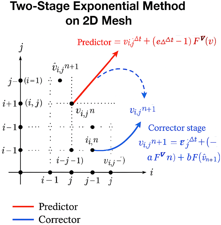
Figure 1: Two-stage exponential method on 2D Mesh
Predictor Stage (Red Arrow, Solid Line): The arrow from
Corrector Stage (Blue Arrows): There are two arrows shown: One solid blue arrow leading to the final point
The Fourier series or Von Neumann stability analysis is used in the literature to determine the stability conditions of finite difference schemes. The analysis is based on certain transformations that will be substituted into the given difference equations. This criterion provides conditions on the Step size and contained parameters in partial differential equations. For nonlinear differential equations, it provides estimates for the actual stability. For this case, the transformations can be expressed as:
By using corresponding transformations from Eqs. (18)–(23) into the first stage of the scheme, and simplification is obtained
Rewrite Eq. (24) as
where
By substituting corresponding transformations from (18)–(23) into third stage of the scheme, it yields
Rewrite Eq. (26) as
where
By using Eq. (25) in Eq. (27), which yields
which can be re-written as
where
The amplitude factor, in this case, is
Thus, the proposed time integrator scheme will remain stable if it satisfies the inequality (29). Therefore, for a stable solution of partial differential equations, the temporal-spatial Step sizes should be chosen adequately so that inequality (29) is satisfied.
Next, in this work, the convergence condition for the system of convection-diffusion equations will be determined. To start this procedure, consider the following system of equations.
where
The proposed scheme for time and space discretization of Eq. (30) can be written as
Theorem 1: The proposed time exponential integrator scheme converges for the vector-matrix Eq. (30).
Proof: The proof of the theorem starts by considering the exact scheme for Eq. (30), which is expressed as:
□
By subtracting Eq. (31) from (33) and considering
etc.
By taking
Rewrite Eq. (36) as
where
Now subtracting (32) from (34), it results in
By taking
By using inequality (37) in (39), the resulting inequality can be rewritten as
where
Let
Since
Let
If this is continued, then for finite
By applying the
Think of the tangent hyperbolic fluid flowing over the flat and oscillating sheets as an unstable, incompressible, laminar non-Newtonian flow in two dimensions. When a plate suddenly moves across a fluid, creating a temperature gradient, the fluid begins to flow. Let
Flow Assumptions: The following is a point-wise list of the flow assumptions for this study.
1. The fluid considered is incompressible, viscous, non-Newtonian, modelled using the tangent hyperbolic fluid framework.
2. The flow is unsteady, two-dimensional, and over a vertical flat/oscillatory plate (without a porous matrix).
3. A uniform magnetic field is applied (normal or inclined as specified), with finite fluid electrical conductivity; the Lorentz force appears in the momentum equation.
4. The fluid exhibits thermal and solutal buoyancy forces, represented by the thermal Grashof number and mass Grashof number.
5. The boundary conditions include oscillatory wall motion, specifically a time-dependent wall velocity in the horizontal direction.
6. The effects of Joule heating and viscous dissipation are accounted for via the Eckert number.
7. The flow assumes no-slip and no-penetration conditions at the wall.
8. Radiative heat transfer and chemical reaction effects are included through appropriate source terms in the energy and species equations.
9. The physical properties (such as viscosity and thermal conductivity) are assumed to be constant throughout the domain, except where variations arise due to the tangent hyperbolic fluid behaviour.
Fig. 2 illustrates the physical setup of tangent hyperbolic fluid flow over an oscillatory flat sheet under a magnetic field. The
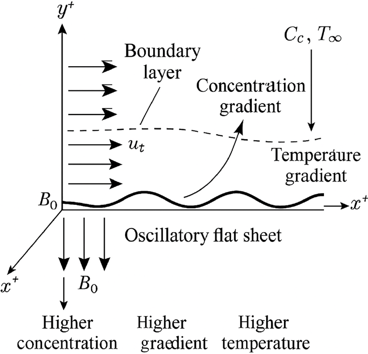
Figure 2: Geometry of the problem
The governing equations of the present model are developed based on established formulations in non-Newtonian fluid mechanics and heat and mass transfer theory. The momentum equation incorporates tangent hyperbolic fluid and magnetic field effects [33], as well as buoyancy-induced thermal convection [34]. The energy equation accounts for temperature-dependent thermal conductivity [35] and viscous dissipation [36], while the species concentration equation includes a first-order chemical reaction term consistent with earlier studies [37]. These modelling choices align with previous literature and form a generalized framework for analyzing complex thermo-fluid systems in porous media. Considering the effects of viscous dissipation and chemical reaction, and temperature-dependent thermal conductivity, the governing equations of the flow can be expressed as:
Each equation employed in the Formulation of the problem is explained below:
Continuity Eq. (45): This is the mass conservation equation for an incompressible fluid in 2D.
Momentum Eq. (46):
Energy Equation (Heat Transfer) (47):
Concentration Equation (Mass Transfer) (48):
subject to initial and boundary conditions
Initial and Boundary Conditions (49): The Fluid is stationary with ambient temperature and concentration. At the
Where
Non-Dimensionalization Eq. (50): To reduce (45)–(49) into dimensionless partial differential equations, consider the following transformations
This process simplifies the equations and introduces dimensionless parameters that govern the flow behaviour.
By employing transformations (50) into Eqs. (45)–(49). The dimensionless governing equations can be written as (See the Appendix A for their proof)
Subject to the dimensionless initial and boundary conditions
where
The skin friction coefficients, which measure wall shear stress, and the local Sherwood number, which measures mass transfer at the wall, are defined as:
here,
where
6 Numerical Results and Discussion
We conduct a comprehensive simulation study with the following aims:
1. Develop and demonstrate a two-stage explicit time integrator (predictor-corrector type) to modify existing exponential integrators for solving nonlinear parabolic PDEs. The predictor stage estimates the intermediate solution, and the corrector stage updates the solution using the predicted value.
2. Establish the stability of the fully discrete scheme for scalar convection-diffusion equations by applying the von Neumann (Fourier) stability analysis, ensuring that the method remains stable for suitable Step sizes and parameter choices.
3. Incorporate high-order compact spatial discretization (fourth or sixth-order accurate) to improve spatial accuracy. The performance of the compact scheme depends on the choice of parameters embedded in the discretization matrices.
4. Prove second-order accuracy in time by matching the Taylor series expansion coefficients in the scheme construction, ensuring theoretical temporal consistency. The vanishing of second derivative terms in time confirms the second-order accuracy of the integrator.
5. Verify convergence of the scheme based on Lax’s equivalence theorem, which holds due to the consistency and stability of the numerical method, ensuring reliable simulation results for mixed convective non-Newtonian flows.
6.1 Effect of Different Parameters on Velocity Profile
Fig. 3a illustrates the impact of the Weissenberg number
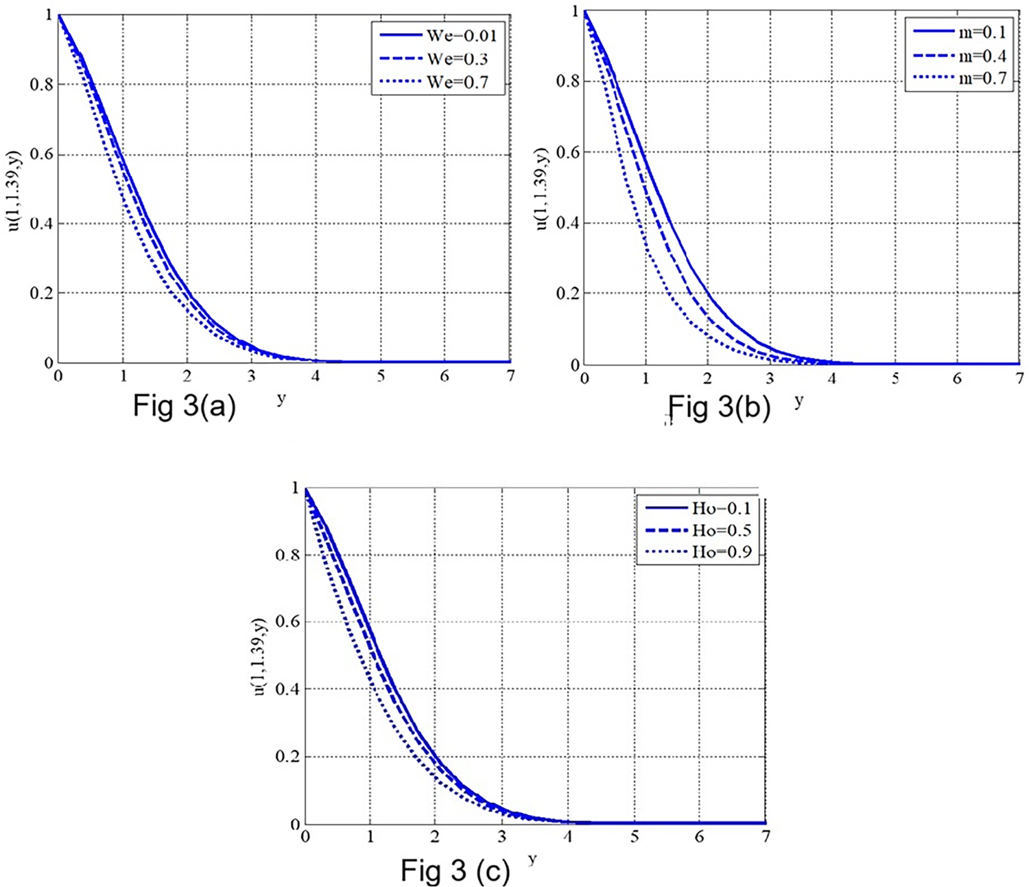
Figure 3: Velocity profile variation under the influence of different physical parameters. (a) Effect of Weissenberg number
Fig. 3b illustrates the effect of the material power-law index
Fig. 3c illustrates the effect of the Hartmann number
6.2 Influence of Eckert Number and Small Parameter on Temperature Profile
Fig. 4a illustrates the effect of the Eckert number
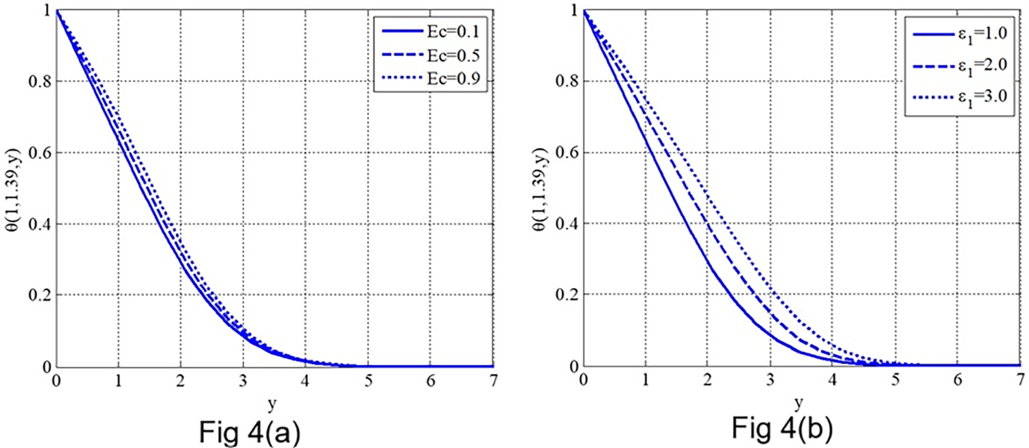
Figure 4: Temperature profile variation with (a) Eckert number
Fig. 4b illustrates the effect of the small parameter
6.3 Concentration and Skin Friction
Fig. 5a depicts the influence of the response rate parameter
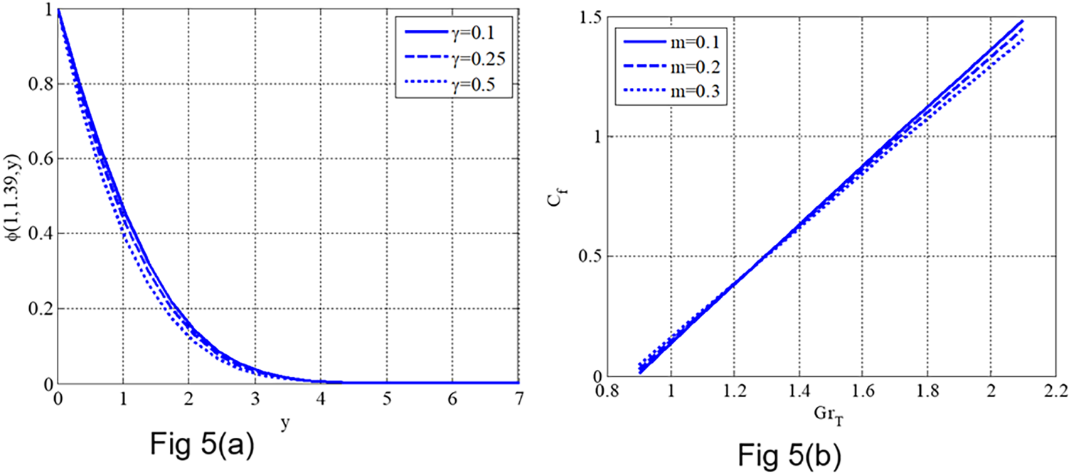
Figure 5: (a) Concentration profile variation with the reaction rate parameter
Fig. 5b illustrates the combined effect of the thermal Grashof number
6.4 Reaction Rate Parameter
Fig. 6 depicts the influence of the Schmidt number.
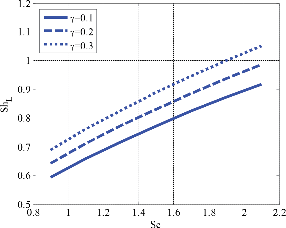
Figure 6: Effect of Schmidt number and reaction rate parameter on local Sherwood number using
6.5 Contour and Mesh Plot Analysis
Figs. 7–9 illustrate the spatio-temporal evolution of the horizontal velocity and temperature profiles for a tangent hyperbolic non-Newtonian fluid over an oscillatory sheet, subject to magnetohydrodynamic and thermal effects. The simulations are performed with the following fixed parameters:
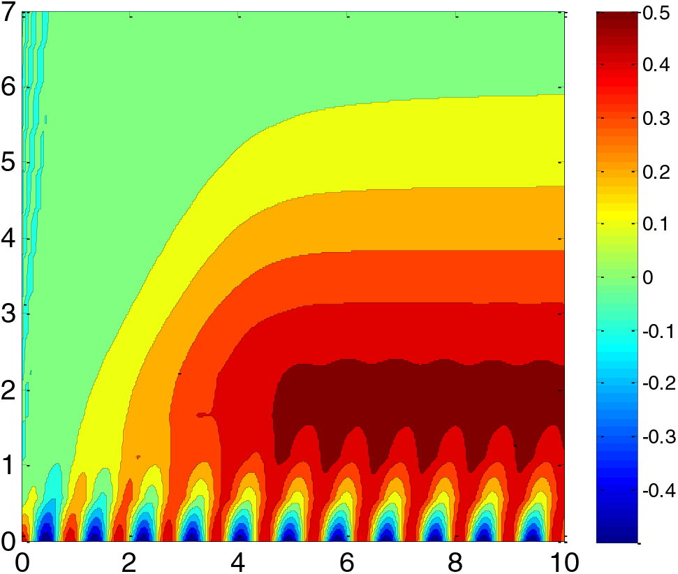
Figure 7: Contour plot for the horizontal component of velocity profile along spatial and temporal coordinates using
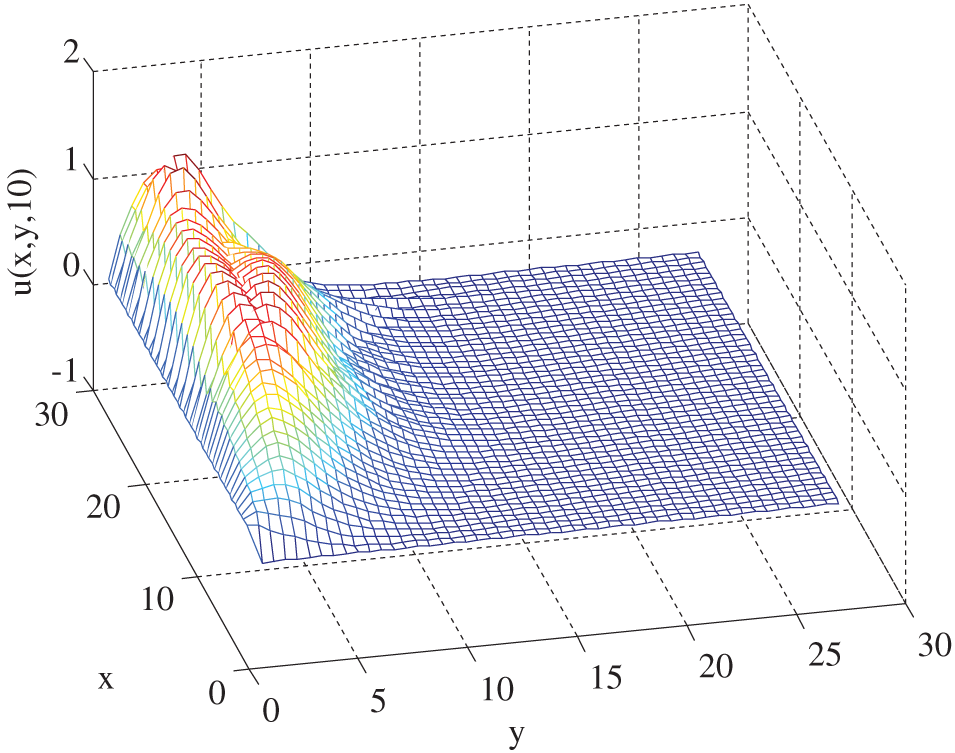
Figure 8: Mesh plot for horizontal component of velocity profile along spatial coordinates using
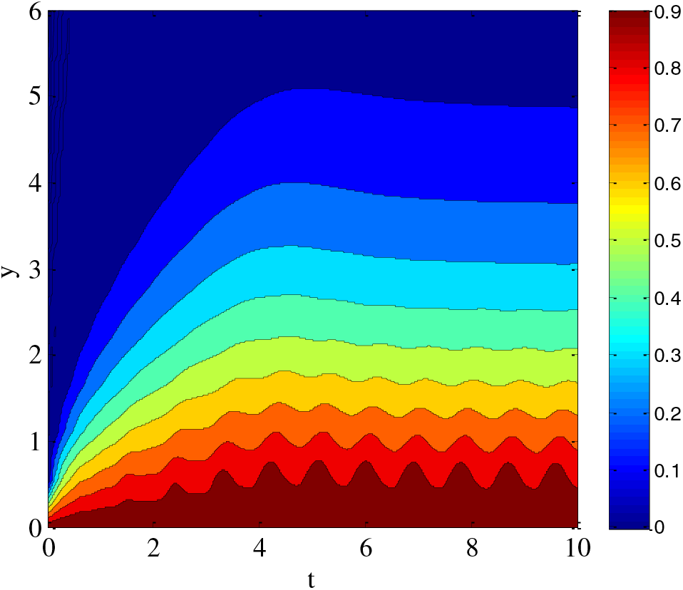
Figure 9: Contour plot for temperature profile along spatial coordinates using
Fig. 7: Contour Plot of Horizontal Velocity
Fig. 8: 3D Mesh Plot of Horizontal Velocity Along Spatial Coordinates: Fig. 8 displays the spatial variation of horizontal velocity in the domain at a representative time snapshot. The surface peaks near the wall confirm that the velocity is maximum adjacent to the oscillatory sheet and rapidly decreases away due to viscous and magnetic damping. The regular wave pattern in the
Fig. 9: Contour Plot of Temperature Distribution. Fig. 9 shows the temperature profile across the 2D domain. The highest temperature occurs near the oscillating sheet, where thermal energy is introduced and converted into the domain. The gradient normal to the plate indicates strong conduction effects, while the lateral spread shows the influence of unsteady convective transport. The layered contour pattern is a result of viscous heating (from high
6.6 Table 1: Comparison of Three Numerical Schemes
Table 1 presents a comparative analysis of the

Table 2 presents the thermophysical properties utilised in the current analysis. These values are selected from standard literature and represent the fluid and physical environments modelled in this study.

Comparison with Existing Literature:
Our findings are consistent with and extend previously published work. For example, Partha et al. [11] reported an enhancement in the Nusselt number due to viscous dissipation in exponential stretching surfaces, which aligns with our observation of an 18.6% rise in the Nusselt number with increasing Eckert number. Uma and Koteswara [12] and Naseer et al. [17] studied tangent hyperbolic fluids using spectral relaxation and numerical methods, respectively. Our scheme demonstrates reduced
To perform this test, we solved the governing system using progressively refined grid sizes while keeping all physical parameters constant. The numerical simulations were carried out for four different spatial node densities

As seen from the table, the difference in the solution becomes negligible beyond
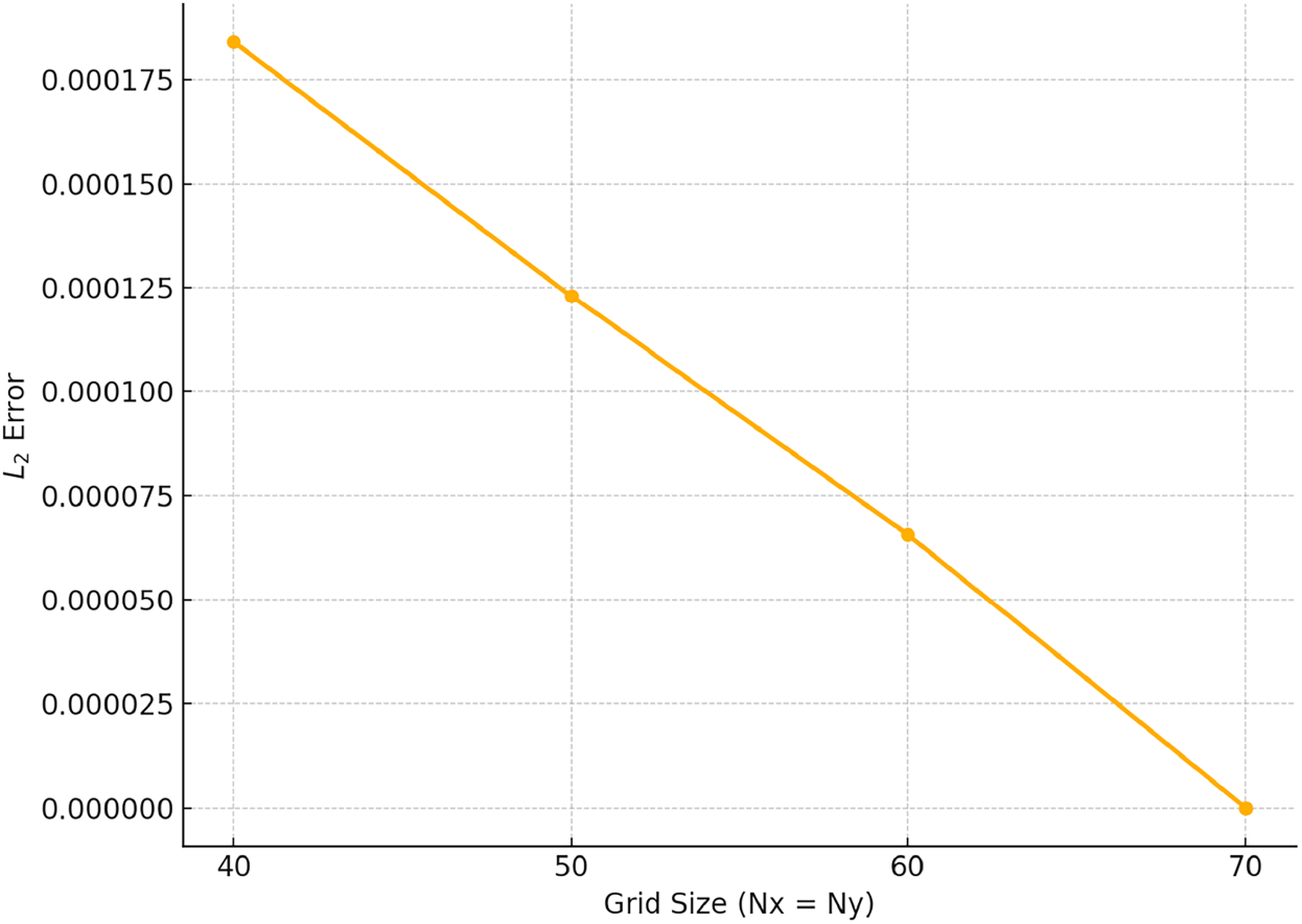
Figure 10: Grid independence test:
6.8 Applications and Practical Relevance
The findings of this work have significant implications in various technical and industrial spheres. Crucially important for managing flow behaviour in polymer extrusion, biofluid dynamics, and food processing systems is the observed reduction in velocity with increasing Weissenberg numbers, reflecting the prevailing viscoelastic characteristic of the tangent hyperbolic fluid. The improvement in skin friction and temperature resulting from the thermal Grashof number suggests the possibility of enhanced thermal management in systems such as nuclear reactors, solar collectors, and electronic device cooling. Furthermore, the rise in local Sherwood number with increased Schmidt number and reaction rate parameter offers valuable information for chemical processing units and reactive flow systems, such as membrane reactors and catalytic converters. Particularly where non-Newtonian fluids are used under magnetic fields and porous media conditions, such as in oil reservoirs, biomedical implants, and industrial heat processing units, these results can directly inform the design of heat exchangers, filtration units, and electromagnetic flow control systems in real-world settings.
This study presents an effective numerical framework to address the complex issue of mixed convective tangent hyperbolic fluid flow over flat and oscillatory sheets, while considering the impact of viscous dissipation. To solve parabolic PDEs, we offer a two-stage exponential integrator. For stiff systems in particular, this explicitly stated methodology outperforms conventional explicit methods in terms of stability and guarantees second-order time precision. Compact spatial discretization methods yielded a high level of accuracy for the terms that depend on space. These schemes are crucial for accurately representing the minute spatial changes and gradients of fluid flow. They are necessary for the precise modeling of the behavior of tangent hyperbolic fluids under mixed convective conditions. An exponential integrator is proposed that consists of two stages, with the first stage serving as the predictor and the second stage serving as the corrector. The predictor stage consisted of a first-order exponential integrator. We developed an extensive mathematical model to describe the movement of tangent hyperbolic fluids over flat and oscillatory surfaces. This model incorporated the influences of viscous dissipation and mixed convection, leading to a set of dimensionless partial differential equations that thoroughly describe the fluid’s dynamics. The divergence-free condition of the continuity equation, which can be challenging to handle, was effectively managed using first-order techniques. This method guaranteed the preservation of mass conservation while maintaining the overall precision and stability of the numerical solution. The scheme was applied to the dimensionless flow model over the moving sheets under the effects of heat and mass transfer. The scheme was also compared with existing schemes. An in-depth analysis was conducted to assess the stability of the proposed two-stage exponential integrator for scalar parabolic equations. The convergence requirements for systems of parabolic equations were obtained, which offer theoretical confirmation of the numerical method’s dependability and resilience. In summary, the arguments might be stated as:
• The proposed two-stage exponential integrator demonstrated superior performance by achieving significantly lower
• A noticeable decline in the velocity profile was observed with increasing Weissenberg number, emphasizing the influence of fluid elasticity in resisting motion.
• The skin friction coefficient increased with higher values of the thermal Grashof number, reflecting enhanced momentum transport due to buoyancy-induced forces near the boundary.
• An upward trend in the local Sherwood number was recorded with increasing Schmidt number and reaction rate parameter, indicating intensified mass transfer in response to reduced molecular diffusion and more vigorous chemical activity.
The goal of this study is to understand a two-dimensional fluid flow. It would make sense to further develop this numerical method for three dimensions, allowing analysis of complex yet authentic fluid dynamical problems. There is room for other things to be studied, for example, magnetic fields, chemical reactions, or state changes. These variables are often highly relevant in reality and can significantly affect how a fluid behaves.
The proposed two-stage exponential integrator and concise spatial discretisation represent a significant advancement in the computational simulation of non-Newtonian fluid dynamics. Applying this strategy to the tangent hyperbolic fluid model on both flat and oscillatory sheets demonstrates its ability to effectively manage complex boundary conditions and nonlinearities. The findings of this study provide valuable insights and tools for addressing various challenges associated with fluid dynamics, thereby promoting further progress in computational fluid dynamics [39,40].
Strengths and Limitations: The proposed two-stage exponential integrator, combined with compact spatial discretization, demonstrates improved accuracy and numerical stability for simulating mixed convective flows of tangent hyperbolic fluids over flat and oscillatory sheets. The scheme effectively reduces
Future Scope: The present study opens several avenues for future research. Potential extensions include the three-dimensional modelling of tangent hyperbolic fluid flow with more complex boundary conditions or geometries to simulate real-world systems more precisely, the incorporation of thermal radiation in variable-property fluids, and investigation under transient magnetic fields for advanced energy systems. Coupling biological or reactive solute transport models makes the framework applicable to biomedical engineering, such as drug delivery through porous tissues. Optimization studies using AI-assisted solvers or surrogate models to minimise energy loss in electro-osmotic microfluidic devices: Experimental validation and prototype testing of the proposed numerical scheme using physical microchannel or porous media setups.
Acknowledgement: This research was supported by the Deanship of Scientific Research, Imam Mohammad Ibn Saud Islamic University (IMSIU), Saudi Arabia.
Funding Statement: This work was supported and funded by the Deanship of Scientific Research at Imam Mohammad Ibn Saud Islamic University (IMSIU) (grant number IMSIU-DDRSP2503).
Author Contributions: Conceptualization, methodology, and analysis, Yasir Nawaz; funding acquisition, Nabil Kerdid; investigation, Muhammad Shoaib Arif; methodology, Mairaj Bibi; project administration, Nabil Kerdid; resources, Mairaj Bibi; supervision, Muhammad Shoaib Arif; visualization, Nabil Kerdid; writing—review and editing, Muhammad Shoaib Arif; proofreading and editing, Nabil Kerdid. All authors reviewed the results and approved the final version of the manuscript.
Availability of Data and Materials: The manuscript included all required data and the implementation of information.
Ethics Approval: Not applicable.
Conflicts of Interest: The authors declare no conflicts of interest to report regarding the present study.
Nomenclature/Dimensionless Quantities
| Nomenclature | ||
| Symbol | Description | Units |
| Velocity components in the | | |
| Temperature | ||
| Concentration | ||
| Spatial coordinates | ||
| Time | ||
| Fluid density | ||
| Dynamic viscosity | ||
| Kinematic viscosity | ||
| Thermal conductivity | ||
| Specific heat at constant pressure | ||
| Electrical conductivity | ||
| Thermal expansion coefficient | ||
| Concentration expansion coefficient | ||
| Mass diffusivity | ||
| Relaxation time for tangent hyperbolic fluid | ||
| Wall velocity | ||
| Domain length in | ||
| Final simulation time | ||
| Shear stress component | ||
| Dimensionless Quantities | ||
| Symbol | Description | Type |
| Hartmann number (magnetic field strength parameter) | Dimensionless | |
| Reynolds number | Dimensionless | |
| Weissenberg number (elasticity parameter of tangent hyperbolic fluid) | Dimensionless | |
| Prandtl number | Dimensionless | |
| Schmidt number | Dimensionless | |
| Thermal Grashof number | Dimensionless | |
| Eckert number | Dimensionless | |
| Thermal radiation parameter | Dimensionless | |
| Small parameter used in numerical scheme or perturbation | Dimensionless | |
| Material power-law index | Dimensionless | |
| Reaction rate parameter | Dimensionless | |
| Non-dimensional temperature | Dimensionless | |
| Non-dimensional concentration | Dimensionless | |
| Skin friction coefficient | Dimensionless | |
| Sherwood number (local mass transfer rate) | Dimensionless | |
| Nusselt number (local heat transfer rate) | Dimensionless | |
This appendix provides detailed steps to derive the dimensionless forms of the governing equations (Eqs. (51)–(54)) from their dimensional forms (Eqs. (45)–(48)), using the scaling transformations introduced in Eq. (50).
Appendix A.1 Scaling and Non-Dimensional Variables
Let the dimensionless variables be defined as:
Using these transformations, the spatial and temporal derivatives transform as:
Appendix A.2 Non-Dimensional Continuity Equation
The dimensional form is:
Using the transformations, this becomes:
Now substitute back into the continuity equation:
Since
This is the dimensionless continuity equation.
Appendix A.3 Non-Dimensional Momentum Equation
The dimensional form Eq. (46) is:
Apply transformations
We also use
Transform Each Term (Just the Key Terms):
Factor out
Appendix A.4 Non-Dimensional Energy Equation
The dimensional form is:
Use
Apply the chain rule to the conduction term and scale all expressions accordingly. After simplifications and using non-dimensional definitions:
Appendix A.5 Non-Dimensional Concentration Equation
The dimensional concentration equation is:
Use
Now use the transformation chain rule:
References
1. Iqra T, Nadeem S, Ali Ghazwani H, Duraihem FZ, Alzabut J. Instability analysis for MHD boundary layer flow of nanofluid over a rotating disk with anisotropic and isotropic roughness. Heliyon. 2024;10(6):e26779. doi:10.1016/j.heliyon.2024.e26779. [Google Scholar] [PubMed] [CrossRef]
2. Patil M, Mahesha, Raju CSK. Convective conditions and dissipation on Tangent Hyperbolic fluid over a chemically heating exponentially porous sheet. Nonlinear Eng. 2019;8(1):407–18. doi:10.1515/nleng-2018-0003. [Google Scholar] [CrossRef]
3. Nadeem S, Akram S. Magnetohydrodynamic peristaltic flow of a hyperbolic tangent fluid in a vertical asymmetric channel with heat transfer. Acta Mech Sin. 2011;27(2):237–50. doi:10.1007/s10409-011-0423-2. [Google Scholar] [CrossRef]
4. Gaffar SA, Prasad VR, Bég OA. Numerical study of flow and heat transfer of non-Newtonian Tangent Hyperbolic fluid from a sphere with Biot number effects. Alex Eng J. 2015;54(4):829–41. doi:10.1016/j.aej.2015.07.001. [Google Scholar] [CrossRef]
5. Gnaneswara Reddy M, Manjula J, Padma P. Mass transfer flow of MHD radiative tangent hyperbolic fluid over a cylinder: a numerical study. Int J Appl Comput Math. 2017;3(1):447–72. doi:10.1007/s40819-017-0364-y. [Google Scholar] [CrossRef]
6. Xu H, Liao SJ. Laminar flow and heat transfer in the boundary-layer of non-Newtonian fluids over a stretching flat sheet. Comput Math Appl. 2009;57(9):1425–31. doi:10.1016/j.camwa.2009.01.029. [Google Scholar] [CrossRef]
7. Megahed AM. Flow and heat transfer of a non-Newtonian power-law fluid over a non-linearly stretching vertical surface with heat flux and thermal radiation. Meccanica. 2015;50(7):1693–700. doi:10.1007/s11012-015-0114-3. [Google Scholar] [CrossRef]
8. Gnaneswara Reddy M, Padma P, Shankar B. Effects of viscous dissipation and heat source on unsteady MHD flow over a stretching sheet. Ain Shams Eng J. 2015;6(4):1195–201. doi:10.1016/j.asej.2015.04.006. [Google Scholar] [CrossRef]
9. Choudhary MK, Chaudhary S, Sharma R. Unsteady MHD flow and heat transfer over a stretching permeable surface with suction or injection. Procedia Eng. 2015;127:703–10. doi:10.1016/j.proeng.2015.11.371. [Google Scholar] [CrossRef]
10. Hussain A, Malik MY, Salahuddin T, Rubab A, Khan M. Effects of viscous dissipation on MHD tangent hyperbolic fluid over a nonlinear stretching sheet with convective boundary conditions. Results Phys. 2017;7:3502–9. doi:10.1016/j.rinp.2017.08.026. [Google Scholar] [CrossRef]
11. Partha M, Murthy P, Rajasekhar G. Effect of viscous dissipation on the mixed convection heat transfer from an exponentially stretching surface. Heat Mass Transf. 2005;41(4):360–6. doi:10.1007/s00231-004-0552-2. [Google Scholar] [CrossRef]
12. Uma K, Koteswara G. Boundary layer flow of MHD tangent hyperbolic fluid past a vertical plate in the presence of thermal dispersion using spectral relaxation method. Int J Math Arch. 2017;8(3):28–41. [Google Scholar]
13. Mamatha SU, Mahesha, Raju CSK, Makinde OD. Effect of convective boundary condition on MHD carreau dusty fluid over a stretching sheet with heat source. Defect Diffus Forum. 2017;377:233–41. doi:10.4028/www.scientific.net/ddf.377.233. [Google Scholar] [CrossRef]
14. Gaffar SA, Prasad VR, Reddy SK, Bég OA. Magnetohydrodynamic free convection boundary layer flow of non-Newtonian tangent hyperbolic fluid from a vertical permeable cone with variable surface temperature. J Braz Soc Mech Sci Eng. 2017;39(1):101–16. doi:10.1007/s40430-016-0611-x. [Google Scholar] [CrossRef]
15. Raju CSK, Sandeep N, Sugunamma V, Jayachandra Babu M, Ramana Reddy JV. Heat and mass transfer in magnetohydrodynamic Casson fluid over an exponentially permeable stretching surface. Eng Sci Technol Int J. 2016;19(1):45–52. doi:10.1016/j.jestch.2015.05.010. [Google Scholar] [CrossRef]
16. Dessie H, Kishan N. MHD effects on heat transfer over stretching sheet embedded in porous medium with variable viscosity, viscous dissipation and heat source/sink. Ain Shams Eng J. 2014;5(3):967–77. doi:10.1016/j.asej.2014.03.008. [Google Scholar] [CrossRef]
17. Naseer M, Malik MY, Nadeem S, Rehman A. The boundary layer flow of hyperbolic tangent fluid over a vertical exponentially stretching cylinder. Alex Eng J. 2014;53(3):747–50. doi:10.1016/j.aej.2014.05.001. [Google Scholar] [CrossRef]
18. Arif MS, Abodayeh K, Nawaz Y. Dynamic simulation of non-Newtonian boundary layer flow: an enhanced exponential time integrator approach with spatially and temporally variable heat sources. Open Phys. 2024;22(1):20240034. doi:10.1515/phys-2024-0034. [Google Scholar] [CrossRef]
19. Abel MS, Datti PS, Mahesha N. Flow and heat transfer in a power-law fluid over a stretching sheet with variable thermal conductivity and non-uniform heat source. Int J Heat Mass Transf. 2009;52(11–12):2902–13. doi:10.1016/j.ijheatmasstransfer.2008.08.042. [Google Scholar] [CrossRef]
20. Jyothi S, Reddy MVS, Gangavathi P. Hyperbolic tangent fluid flow through a porous medium in an inclined channel with peristalsis. Int J Math Trends Technol. 2016;1(1):113–21. doi:10.26643/gis.v15i1.18705. [Google Scholar] [CrossRef]
21. Vendabai GSK. Unsteady convective boundary layer flow of a nanofluid over a stretching surface in the presence of a magnetic field and heat generation. Int J Emerg Trends Eng Dev. 2014;3:214–30. doi:10.1017/CBO9781107415324.004. [Google Scholar] [CrossRef]
22. Mansur S, Ishak A. Unsteady boundary layer flow of a nanofluid over a stretching/shrinking sheet with a convective boundary condition. J Egypt Math Soc. 2016;24(4):650–5. doi:10.1016/j.joems.2015.11.004. [Google Scholar] [CrossRef]
23. Sarojamma G, Vendabai K. Boundary layer flow of a Casson nanofluid past a vertical exponentially stretching cylinder in the presence of a transverse magnetic field with internal heat generation/absorption. Int J Mech Aerospace Ind Mechatronics Eng. 2015;9(7):138–43. doi:10.1007/s13204-013-0267-0. [Google Scholar] [CrossRef]
24. Khoshrouye Ghiasi E, Saleh R. A convergence criterion for tangent hyperbolic fluid along a stretching wall subjected to inclined electromagnetic field. Sema J. 2019;76(3):521–31. doi:10.1007/s40324-019-00190-1. [Google Scholar] [CrossRef]
25. Gorla RSR, Chamkha A. Natural convective boundary layer flow over a nonisothermal vertical plate embedded in a porous medium saturated with a nanofluid. Nanoscale Microscale Thermophys Eng. 2011;15(2):81–94. doi:10.1080/15567265.2010.549931. [Google Scholar] [CrossRef]
26. Chamkha AJ, Rashad AM. Unsteady heat and mass transfer by MHD mixed convection flow from a rotating vertical cone with chemical reaction and Soret and Dufour effects. Can J Chem Eng. 2014;92(4):758–67. doi:10.1002/cjce.21894. [Google Scholar] [CrossRef]
27. Rashad AM, Abdou MMM, Chamkha A. MHD free convective heat and mass transfer of a chemically-reacting fluid from radiate stretching surface embedded in a saturated porous medium. Int J Chem React Eng. 2011;9(1):1–15. doi:10.1515/1542-6580.2501. [Google Scholar] [CrossRef]
28. Arif MS, Shatanawi W, Nawaz Y. A computational framework for electro-osmotic flow analysis in Carreau fluids using a hybrid numerical scheme. Int J Thermofluids. 2025;27(Suppl. 2):101240. doi:10.1016/j.ijft.2025.101240. [Google Scholar] [CrossRef]
29. Nawaz Y, Arif MS, Abodayeh K, Ashraf MU. Modeling viscous dissipation in MHD boundary layer flow: a two-stage in time and compact in space finite difference approach. Numer Heat Transf Part B Fundam. 2024;2024:1–30. doi:10.1080/10407790.2024.2338904. [Google Scholar] [CrossRef]
30. Shoaib M, Khan RA, Ullah H, Nisar KS, Raja MAZ, Islam S, et al. Heat transfer impacts on Maxwell nanofluid flow over a vertical moving surface with MHD using stochastic numerical technique via artificial neural networks. Coatings. 2021;11(12):1483. doi:10.3390/coatings11121483. [Google Scholar] [CrossRef]
31. Ullah H, Khan I, AlSalman H, Islam S, Asif Zahoor Raja M, Shoaib M, et al. Levenberg-marquardt backpropagation for numerical treatment of micropolar flow in a porous channel with mass injection. Complexity. 2021;2021(1):5337589. doi:10.1155/2021/5337589. [Google Scholar] [CrossRef]
32. Rehman KU, Shatanawi W, Alharbi WG, Shatnawi TAM. AI-Neural Networking Analysis (NNA) of thermally slip magnetized Williamson (TSMW) fluid flow with heat source. Case Stud Therm Eng. 2024;56(6):104248. doi:10.1016/j.csite.2024.104248. [Google Scholar] [CrossRef]
33. Khan AA, Zafar S, Khan A, Abdeljawad T. Tangent hyperbolic nanofluid flow through a vertical cone: unraveling thermal conductivity and Darcy-Forchheimer effects. Mod Phys Lett B. 2025;39(8):2450398. doi:10.1142/s0217984924503986. [Google Scholar] [CrossRef]
34. Chamkha AJ. Hydromagnetic combined convection flow in a vertical channel. Heat Mass Transf. 2000;36(5):387–93. [Google Scholar]
35. Mahdy A. MHD non-Darcy natural convection heat transfer from a vertical heated plate embedded in a porous medium with variable thermal conductivity. Commun Non-linear Sci Numer Simul. 2012;17(1):130–43. doi:10.1016/j.cnsns.2010.02.003. [Google Scholar] [CrossRef]
36. Makinde OD, Aziz A. Boundary layer flow of a nanofluid past a stretching sheet with a convective boundary condition. Int J Therm Sci. 2011;50(7):1326–32. doi:10.1016/j.ijthermalsci.2011.02.019. [Google Scholar] [CrossRef]
37. Raptis A, Perdikis C. Viscous flow over a non-linearly stretching sheet in the presence of a chemical reaction and magnetic field. Int J Non Linear Mech. 2006;41(4):527–9. doi:10.1016/j.ijnonlinmec.2005.12.003. [Google Scholar] [CrossRef]
38. Li FL, Wu ZK, Ye CR. A finite difference solution to a two-dimensional parabolic inverse problem. Appl Math Model. 2012;36(5):2303–13. doi:10.1016/j.apm.2011.08.025. [Google Scholar] [CrossRef]
39. Kerdid N, Arif MS, Nawaz Y, Abodayeh K. Computational analysis of radiation effects in Williamson fluid flow through a porous medium under an inclined magnetic field. J Radiat Res Appl Sci. 2025;18(2):101499. doi:10.1016/j.jrras.2025.101499. [Google Scholar] [CrossRef]
40. Farooq U, Kerdid N, Nawaz Y, Arif MS. High accuracy simulation of electro-thermal flow for non-Newtonian fluids in BioMEMS applications. Comput Model Eng Sci. 2025;144(1):873–98. doi:10.32604/cmes.2025.066800. [Google Scholar] [CrossRef]
Cite This Article
 Copyright © 2025 The Author(s). Published by Tech Science Press.
This work is licensed under a Creative Commons Attribution 4.0 International License , which permits unrestricted use, distribution, and reproduction in any medium, provided the original work is properly cited.
 Downloads
 Citation Tools