
 Submit a Paper
 Propose a Special lssue
 Open Access
ARTICLE

An Efficient GPU Solver for Maximizing Fundamental Eigenfrequency in Large-Scale Three-Dimensional Topology Optimization
1 School of Mechanical Engineering and Automation, Beihang University, Beijing, 102206, China
2 State Key Laboratory of Virtual Reality Technology and Systems, Beihang University, Beijing, 100191, China
* Corresponding Author: Junpeng Zhao. Email:
(This article belongs to the Special Issue: Topology Optimization: Theory, Methods, and Engineering Applications)
Computer Modeling in Engineering & Sciences 2025, 145(1), 127-151. https://doi.org/10.32604/cmes.2025.070769
Received 23 July 2025; Accepted 09 September 2025; Issue published 30 October 2025
 View Full Text
 Download PDF
Abstract
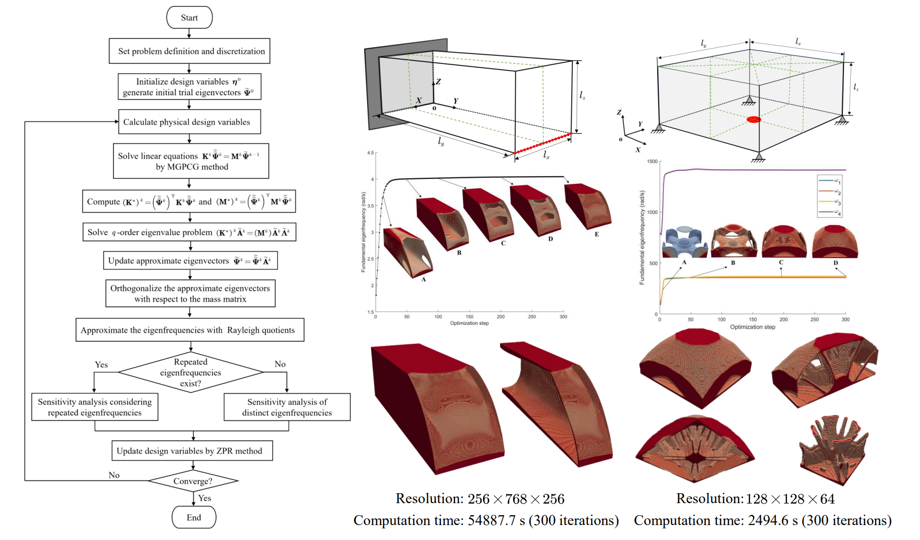
A major bottleneck in large-scale eigenfrequency topology optimization is the repeated solution of the generalized eigenvalue problem. This work presents an efficient graphics processing unit (GPU) solver for three-dimensional (3D) topology optimization that maximizes the fundamental eigenfrequency. The Successive Iteration of Analysis and Design (SIAD) framework is employed to avoid solving a full eigenproblem at every iteration. The sequential approximation of the eigenpairs is solved by the GPU-accelerated multigrid-preconditioned conjugate gradient (MGPCG) method to efficiently improve the eigenvectors along with the topological evolution. The cluster-mean approach is adopted to address the non-differentiability issue caused by repeated eigenfrequencies. The corresponding sensitivity analysis method is provided. The parallelized gradient-based Zhang-Paulino-Ramos Jr. (ZPR) algorithm is employed to update the design variables. The effectiveness of the proposed solver is demonstrated through two large-scale numerical examples. The first example demonstrates the accuracy, efficiency, and scalability of the proposed solver by solving a 3D optimization problem of 50.33 million elements being solved in approximately 15.2 h over 300 iterations on a single NVIDIA Tesla V100 GPU. The second example validates the effectiveness of the proposed solver in the presence of repeated eigenfrequencies. Our findings also highlight that higher-resolution models produce distinct optimized structures with higher fundamental frequencies, underscoring the necessity of large-scale topology optimization.Graphic Abstract
Keywords
In practical engineering, such as spacecraft design, preventing resonance between the primary structure and excitation sources is a critical requirement for launch-phase integrity assurance. One common practice is to maximize the fundamental eigenfrequency of the structure to raise it beyond the dominant excitation spectrum [1–3]. For many applications, relying solely on engineering experience and intuition to achieve this purpose is very challenging. In these situations, topology optimization provides a powerful methodology [4–7].
Topology optimization is a fundamental method to automatically design high-performance structures [8–10]. To date, several topology optimization approaches, such as the homogenization method [11], the density-based approach [12,13], the level-set method [14,15], the evolutionary structural optimization method [16,17], as well as the moving morphable components method [18], have been developed and they have also been widely used in industrial applications [9]. Nevertheless, although substantial progress has been made, topology optimization considering fundamental eigenfrequency is still not an easy task.
Generally speaking, three main difficulties are encountered when solving topology optimization problems for maximizing the fundamental eigenfrequency of continuum structures. Firstly, inappropriate interpolation functions can lead to the emergence of localized modes [19]. This phenomenon can seriously undermine the accuracy and reliability of the solution, as these spurious modes often dominate the lowest eigenfrequencies, masking the true physical behavior of the system. Secondly, the occurrence of repeated eigenfrequencies during the optimization process results in the conventional Fréchet sensitivity becoming undefined [20–22]. Consequently, standard gradient-based optimization algorithms struggle to converge, or may fail entirely, when they encounter such a design. Thirdly, eigenmodes corresponding to different eigenfrequencies may switch their orders during optimization, which leads to discontinuities in the objective function [23,24]. The sudden change in the objective function can cause gradient-based algorithms to oscillate or jump to a suboptimal solution instead of smoothly converging to the optimal one.
To address the issue of localized modes, modifications can be made to the stiffness and mass interpolation functions, such as piecewise interpolation schemes [19,25,26], Rational Approximation of Material Properties (RAMP) interpolation [21], and polynomial penalization methods [27–29]. To resolve the non-differentiability arising from eigenfrequency multiplicities and the associated mode switching, three distinct categories of optimization approaches have been developed. The first category employs directional derivatives and a perturbation method to link eigenfrequency increments to changes in design variables, formulating a sub-problem at each iteration, which can be complicated by additional constraints [26,30–32]. The second category, based on symmetric spectral aggregation, renders the objective function differentiable through functions like the mean eigenvalue,
In practical applications, the main difficulty is the computational challenge. Conventionally, topology optimization is an iterative process. In each optimization step, the nested finite element equations must be solved. However, when the system has a large number of Degrees of Freedom (DOFs), solving the nested finite element equations is prohibitively expensive in terms of computational time. This becomes even worse when performing topology optimization to maximize fundamental eigenfrequency, where a nested generalized eigenvalue problem needs to be solved in each optimization step, which is even harder than static problems [38].
In order to overcome this bottleneck, Andreassen et al. [39] used frequency response surrogates for eigenvalue optimization problems in topology optimization to avoid solving the generalized eigenvalue problem. Though this method offers an alternative to solving the eigenvalue maximization problem without having to actually compute eigenvalues, the excitation frequency must be chosen carefully because the frequency response strongly depends on the spatial distribution and the frequencies of the external excitations. Ferrari et al. [38] extended and enhanced the method by introducing a strategy based on multilevel discretizations. This strategy accurately computes eigenvalues and eigenvectors only on the coarsest discretization and then performs inexpensive operations to recover the fine-scale harmonic loads and solve the fine-scale linear system. Thus, the efficiency of the solution procedure has been significantly improved. To mitigate the computational burden associated with large-scale eigenvalue analysis, Leader et al. [33] implemented a Jacobi–Davidson solver designed for iterative frameworks. Their contribution includes a specialized strategy for reusing eigenvectors, enabling efficient topology optimization at high resolutions under frequency constraints. The efficacy of this combined methodology was validated on a mass minimization design problem for a cantilever beam, incorporating both stress and frequency limitations, and involving 42.7 million DOFs. To enhance solution efficiency in compliance and eigenfrequency optimization, Fu and Kennedy [40] developed a tailored quasi-Newton correction scheme. Their approach leverages problem-dependent second-order derivatives to eliminate detrimental curvature components, thereby improving optimization convergence. Validation included large-scale modal analysis cases exceeding 15.5 million DOFs, confirming the robustness of the method for frequency-constrained problems.
Kang et al. [41] proposed a successive iteration of analysis and design (SIAD) method for solving large-scale eigenvalue topology optimization problems. This novel method is developed based on the concept of sequential approximation that has been successfully employed to solve reliability-based design problems [42]. The SIAD technique employs iteratively updated vector approximations that converge toward exact eigenvectors during design progression. By circumventing traditional nested iterative frameworks, this approach achieves significant reduction on computational cost. As demonstrated in [41], a 3D cantilever beam design problem with 2.45 million DOFs was solved with 100 iterations in approximately 6.38 h on a workstation with dual Intel@ Xeon@ CPUs (E5-2670v3@2.3 GHz). In conjunction with the idea of SIAD, Shi et al. [43] introduced a multi-stage refinement framework employing relay-based computational strategies. Starting with coarse finite element discretizations, the methodology progressively enhances spatial resolution through systematic mesh refinement. This approach dramatically mitigates computational demands while attaining high-fidelity design boundaries. Their results further validate the computational efficacy and extensibility of the SIAD methodology.
In recent years, GPU (Graphics Processing Unit) cards have become more and more popular in solving topology optimization problems because of their capabilities of performing highly parallel tasks [44,45]. Studies have shown that GPU cards can be used to accelerate the solving of large-scale topology optimization problems, such as structural design [46], inverse homogenization [47], among others. The authors of this work also developed efficient GPU solvers for topology optimization of composite structures with spatially varying fiber orientations [48,49]. These studies clearly demonstrated that unlike the traditional CPU-based parallel strategy, the GPU-based parallel strategy may need much less computational resources when solving problems of the same scale. Topology optimization problems with dozen millions of elements can be solved using only one consumer-grade GPU card [50,51], making GPU-based parallel strategy more available.
This paper proposes an efficient GPU-based solver for maximizing the fundamental eigenfrequency of large-scale 3D structures subject to a volume fraction constraint. Noting that the key computational bottleneck in the SIAD method is to obtain the approximate eigenvector by solving a set of finite element equations mathematically analogous to the governing equations of static equilibrium, the multigrid preconditioned conjugate gradient (MGPCG) method is employed to efficiently solve these finite element equations. In order to accommodate the constraint of limited GPU memory capacity while leveraging the advantage of its massively parallel architecture, the MGPCG method is implemented in a matrix-free way, avoiding the assembly of the global stiffness matrix and large-scale matrix and vector multiplication operations. To resolve the non-differentiability of repeated eigenfrequencies and the associated mode switching, the cluster-mean approach [36] is adopted because it avoids auxiliary constraints and is straightforward to implement within gradient-based optimization frameworks. The corresponding sensitivity analysis method is also presented. We also implement the Zhang-Paulino-Ramos Jr. (ZPR) method in parallel to accelerate the update of design variables. Numerical examples show that 3D topology optimization problem with 50.33 million elements can be solved with 300 iterations in about 15.2 h using one NVIDIA V100 GPU card for maximizing the fundamental eigenfrequency. It is also found that, the true fundamental eigenfrequency optimal design of the cantilever beam problem is different from those obtained in [38,41], closed-walled shell structures with variable thickness appear in the free end of the optimal design. In addition, the effectiveness of the proposed solver in the presence of repeated eigenfrequencies is also demonstrated.
The remainder of this work is organized as follows: Section 2 formulates the structural topology optimization problem for maximizing the fundamental eigenfrequency. Section 3 states the solution method, including a brief introduction of the SIAD method, a GPU accelerated MGPCG solver for solving large-scale finite element equations, sensitivity analysis and ZPR design variable update scheme. Section 4 presents the optimization procedure. Section 5 showcases numerical results demonstrating the practical effectiveness and scalability of our GPU-optimized solver. Finally, conclusions are drawn in the last section.
2 Problem Formulation of Topology Optimization for Maximizing Fundamental Eigenfrequency
2.1 Design Parametrization and Regularization
The classical density-based approach is employed to solve the topology optimization problem. Assume the design domain is meshed into N elements, with volumes
where
When performing topology optimization, the original density variables
2.2 Material Interpolation Scheme
In order to obtain clear topologies, material interpolation schemes are employed. The Young’s modulus and structural density of element
where
where
The topology optimization problem, which aims to maximize the fundamental eigenfrequency by finding the optimal material distribution, is formulated as:
where
Typically, the problem 7 is solved in a double-loop strategy, where in the outer loop, an optimization algorithm such as the method of moving asymptotes (MMA) updates the design variables, while in the inner loop, the generalized eigenvalue problem is solved. However, accurately solving generalized eigenvalue problems presents a computational challenge for large-scale problems. Kang et al. [41] proposed the novel SIAD method, in which concurrent convergence of eigenvalue analysis and design optimization are implemented. The SIAD method allows for an affordable solution to eigenfrequency optimization problems with millions of DOFs that can be completed on a desktop computer. In this section, a GPU-based SIAD framework is proposed for maximizing the fundamental eigenfrequency in large-scale 3D topology optimization, demonstrating significant computational efficiency.
3.1 Brief Description of the SIAD Method
In the SIAD method, in each optimization step, the approximate eigenmodes obtained in the previous step are chosen as the initial subspace basis, and then a one-step inverse subspace iteration is performed to sequentially improve the accuracy of the eigenmodes. Considering that the fundamental eigenfrequency may become repeated during the optimization process, apart from the first-order eigenfrequency, some higher-order eigenfrequencies also need to be computed. The subspace iteration method [54] is employed to compute the first several low-order eigenvalues and eigenvectors.
Suppose that the first
where
Then,
After sorting, we use
When the approximate low-order eigenpairs are obtained, sensitivity analysis for design variables can be performed. According to whether the fundamental eigenfrequency is distinct or repeated, the sensitivity needs to be computed in different ways. When the fundamental eigenfrequency is distinct, the design sensitivity in the
Further, substituting the expression of the element stiffness and mass matrices into Eq. (12) yields
where
In the case that the fundamental eigenfrequency in the
Once the objective function is changed into the cluster-mean
It can be found that when the fundamental eigenfrequency is distinct,
Upon computation of sensitivity information, design variables are updated via gradient-based optimization algorithms (e.g., the MMA method or the ZPR algorithm).
The above process iterates until optimization convergence. Crucially, unlike conventional double-loop strategies requiring accurate eigenpair solutions in every optimization iteration, the SIAD method employs approximate eigenpairs that concurrently converge with the optimization process. Although eigenpair accuracy is not enforced at intermediate iterations, they ultimately converge to exact values for the optimized design upon termination. By replacing the generalized eigenvalue problem with Eq. (8) solves, the SIAD method substantially reduces the number of full-scale linear system solutions compared to conventional approaches. Consequently, the SIAD method demonstrates significant efficiency advantages.
Nevertheless, solving Eq. (8) remains computationally challenging for large-scale problems. It should be noted that these equations closely resemble the nested finite element equations in statics problems, differing only in the right-hand side computation. Since the right-hand side computation requires only
3.2 GPU-Accelerated SIAD Method for Maximizing the Fundamental Eigenfrequency
Define
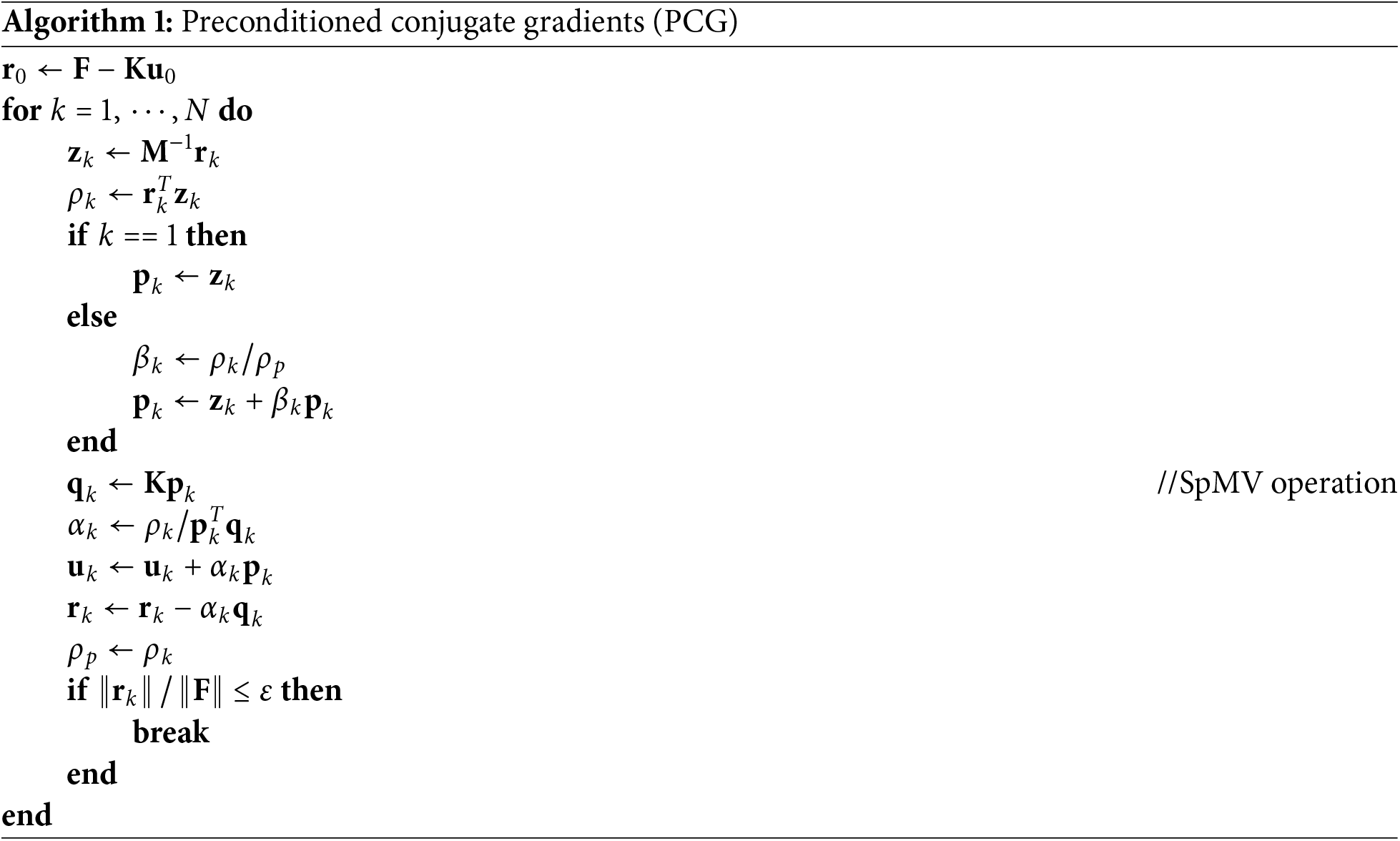
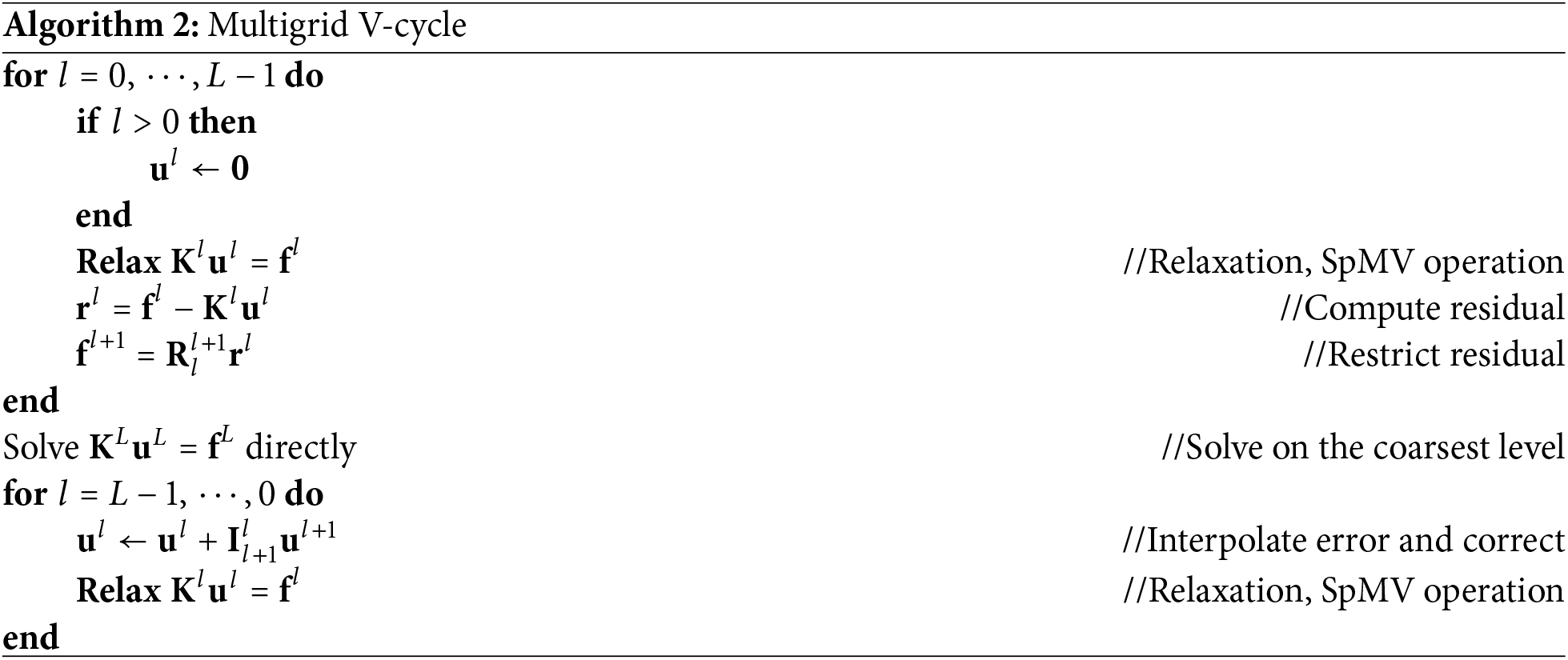
The algorithmic workflow of the MGPCG method is specified through pseudocode in Algorithms 1 and 2. The multigrid V-cycle accelerates the convergence of the CG by employing a hierarchy of nested meshes. High-frequency solution errors are damped through local smoothing operations on fine grids, while persistent low-frequency errors are resolved by restricting residuals to coarser grids. On these coarser scales, such errors become effectively high-frequency and are addressed through recursive or direct solution of the reduced problem. Corrections are then prolongated back to finer grids, systematically reducing errors across all frequency bands.
The primary computational burden in the MGPCG method arises from the Sparse Matrix-Vector Multiplication (SpMV) operations. Within each PCG iteration (Algorithm 1), a minimum of three SpMV operations are required: one for computing
Due to the constrained memory capacity of GPU devices, particularly when using a single GPU as in this study, assembling and storing the global stiffness matrix is impractical. To overcome this limitation, we implement the SpMV operation in a matrix-free way using the Node-by-Node strategy [45]. This method computes the product
where
To minimize device memory footprint, in the multigrid V-cycle, we implement a hierarchical matrix storage strategy where only the coarsest-level stiffness matrix
In our implementation, we use Jacobi relaxation to the system equations at different hierarchies except for the coarsest one with the relaxation factor being chosen as 0.6. For more details of the multigrid V-cycle, it is recommended to refer to [55]. A direct method based on the Cholesky decomposition is employed to solve the system equations at the coarsest hierarchy. The relative residual tolerance of the PCG solver is set as
3.3 ZPR-Based Design Variable Update Strategy
In the SIAD method implemented in [41], the MMA method is employed to update the design variables. However, for problems involving large number of design variables, the execution time of the conventional sequential MMA algorithm becomes computationally intensive. Parallelizing the MMA algorithm for efficient GPU execution is a non-trivial computational undertaking, even though the principle is similar to that proposed in [56]. Instead, the ZPR design variable update scheme is used in this work.
The original version of the ZPR design variable update scheme [57] was formulated for solving the canonical minimum compliance design problems, where the sensitivity of the objective function with respect to the design variables is always negative. However, for non-self-adjoint problems, such as maximum fundamental eigenfrequency design as considered in this study or minimum dynamic response design [58], the sensitivity of the objective function with respect to the design variables may take on positive values. To address this limitation, an extended ZPR-based design variable update scheme compatible with general sensitivity profiles is developed [58]. We will briefly review the extended ZPR-based design variable update scheme in this subsection.
In each optimization step, a convex approximation is constructed to define the approximate sub-problem:
where
are lower and upper bounds on the density design variables, respectively,
where
where
In addition, a diagonal approximation of the Hessian matrix based on the Powell Symmetric Broyden quasi-Newton update is adopted to estimate the second-order sensitivity information at the
where
Finally, in order to improve the robustness of the approach, the density design variable at the
where
This method is inherently highly parallelizable, such that the update process of design variables demonstrates remarkable efficiency in practical implementations. The robustness and extremely low computational cost will be demonstrated through numerical examples in Section 5.
The flowchart in Fig. 1 outlines the topology optimization process for fundamental eigenfrequency maximization using the SIAD method. In each iteration, four steps are performed: first, the physical design variables are calculated; second, the finite element equations are solved by the MGPCG method and the fundamental eigenfrequency is approximated by the Rayleigh quotient; third, a sensitivity analysis is executed; and finally, the design variables are updated using the ZPR method. This iterative process repeats until convergence. For GPU acceleration, all four steps are parallelized.
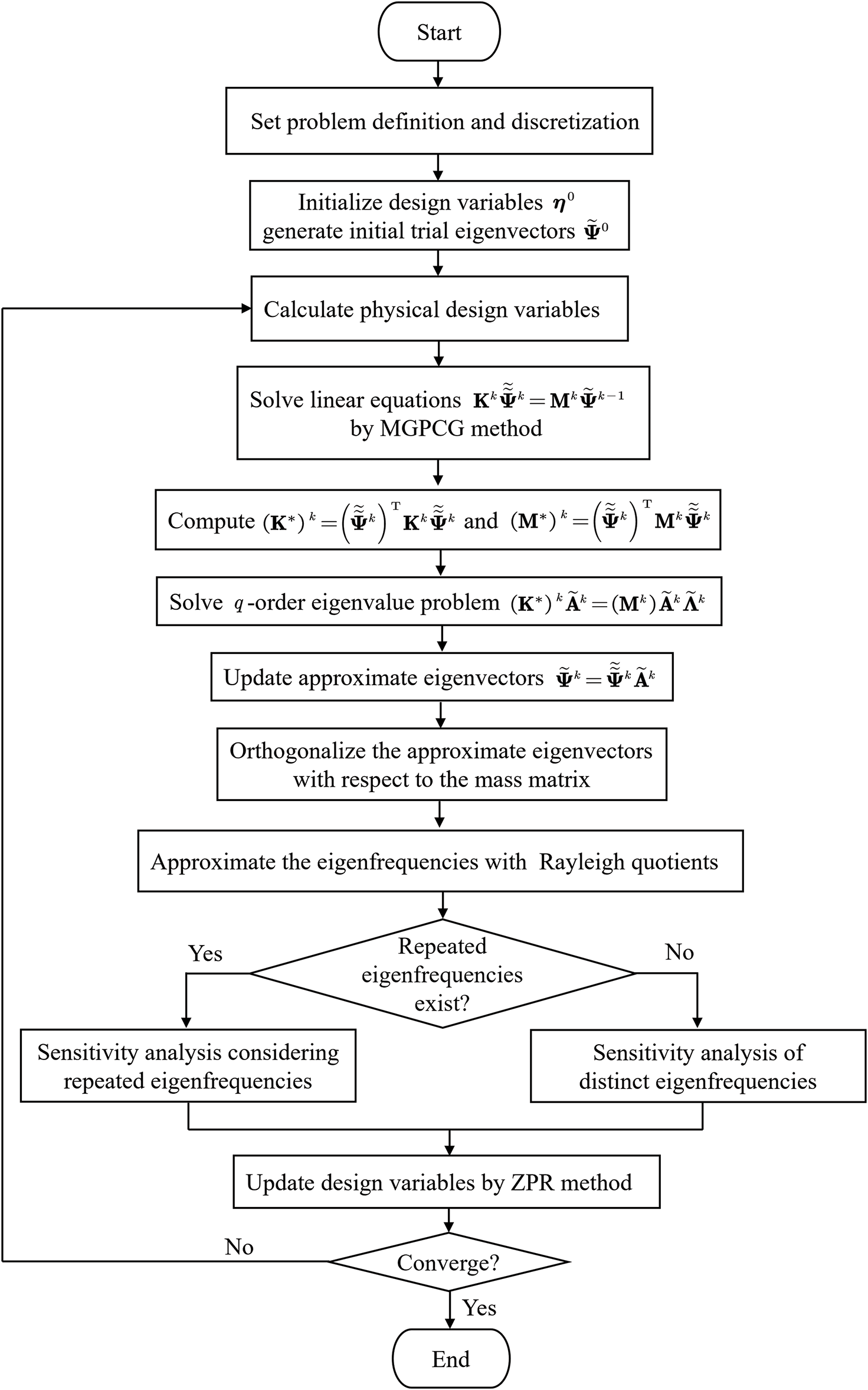
Figure 1: Flowchart for topology optimization to maximize fundamental eigenfrequency
This section presents two numerical examples to illustrate the effectiveness of the proposed GPU solver for maximizing fundamental eigenfrequency in large-scale 3D topology optimization. In both numerical examples, density filter with a radius being 1.5 times the element size is applied. The lumped mass matrix is employed. The symmetry constraint was imposed on the density variables. At the beginning of the optimization process, the material is uniformly distributed throughout the design domain, and randomly generated trial eigenvectors are used. The optimization is terminated upon completion of 300 iterations.
The computations are performed on a compute node within a high-performance computing cluster, equipped with an Intel® Xeon® Gold 6240 Processor and an NVIDIA Tesla V100 GPU. The implementation is carried out using the Taichi 1.7.0 programming language [59]. For visualizing the optimized results, ParaView 5.8.1 [60] is employed. It is notable that the threshold value is set to 0.8 for the density distribution in this work unless otherwise stated.
5.1 Case Study 1: Fundamental Eigenfrequency Maximization of a 3D Cantilever Beam
This numerical experiment is adopted from [41] to quantitatively assess the performance gains achieved by the developed GPU solver. The purpose of this example is to maximize the fundamental eigenfrequency of a 3D cantilever beam while satisfying the material constraint. Fig. 2 illustrates the cuboidal solution domain with spatial extents
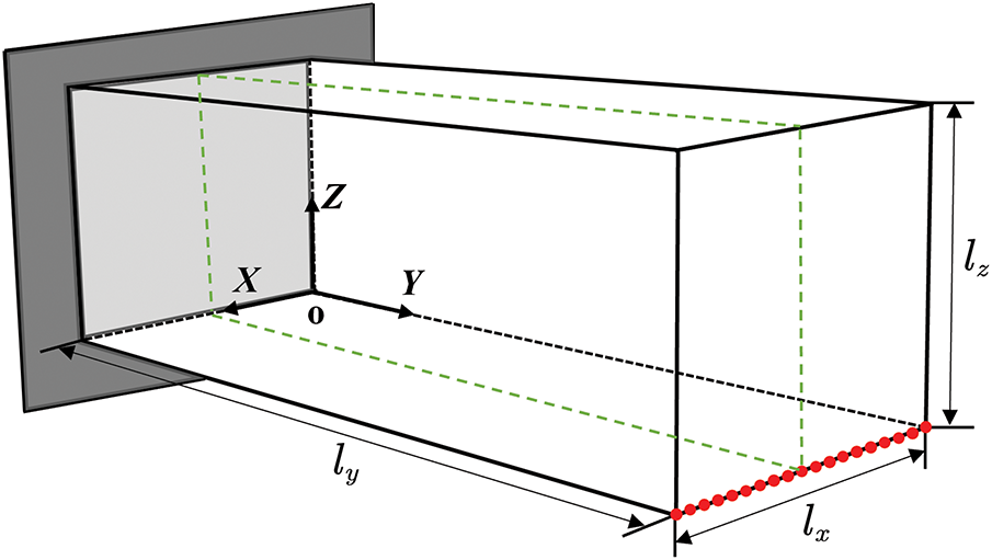
Figure 2: Definition of the 3D cantilever beam design problem
The computational domain is discretized into a structured grid of 64
The final design is plotted in Fig. 3a,b. Both the whole structure and the half one are depicted to show the optimized design and its interior structure. It can be observed that hollow thin-walled characteristic are emerged in the final design. The optimized design is similar to that obtained in [41]. The difference can be attributed to different initializations, different filtering methods, as well as different optimization algorithms. The iteration history of the fundamental eigenfrequency is plotted in Fig. 4. The fundamental eigenfrequency reveals a sustained growth during the optimization iteration, ascending from 1.8115 rad/s at initialization to 4.0391 rad/s upon convergence. Some intermediate designs are also depicted in Fig. 4, the threshold values 0.6 are set for all the displayed density distributions (solution A, B, C, D, E in the 10th, 50th, 100th, 200th and the final optimization step, respectively). As the subspace iteration method uses a subspace size of q = 2, the SIAD method needs to solve two linear systems in each iteration. The iteration history of the number of CG iterations is plotted in Fig. 5. Notably, the maximum steps required for single CG iteration convergence is 51, which makes the computation time of the MGPCG method acceptable. It can be seen that an upward trend of the number of CG iterations presents in the optimization process, which could be attributed to the thin-walled features emerging in the structural evolution. In the later stages of optimization iteration, the structural changes become insignificant, leading to a stabilization in the number of CG iteration.
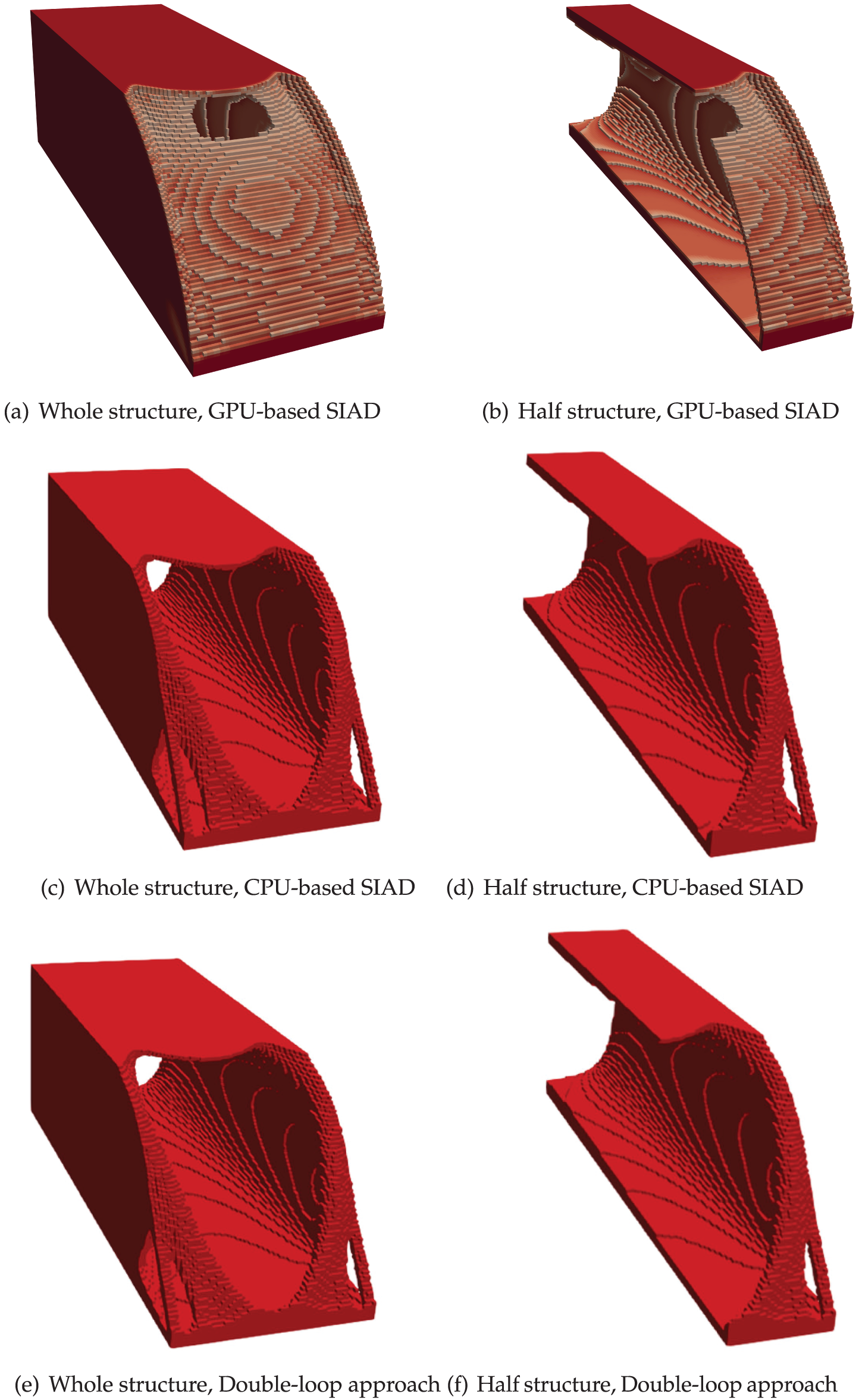
Figure 3: Optimized structure of the 3D cantilever beam. (c–f) Reprinted with permission from Elsevier, from Kang et al. [41]
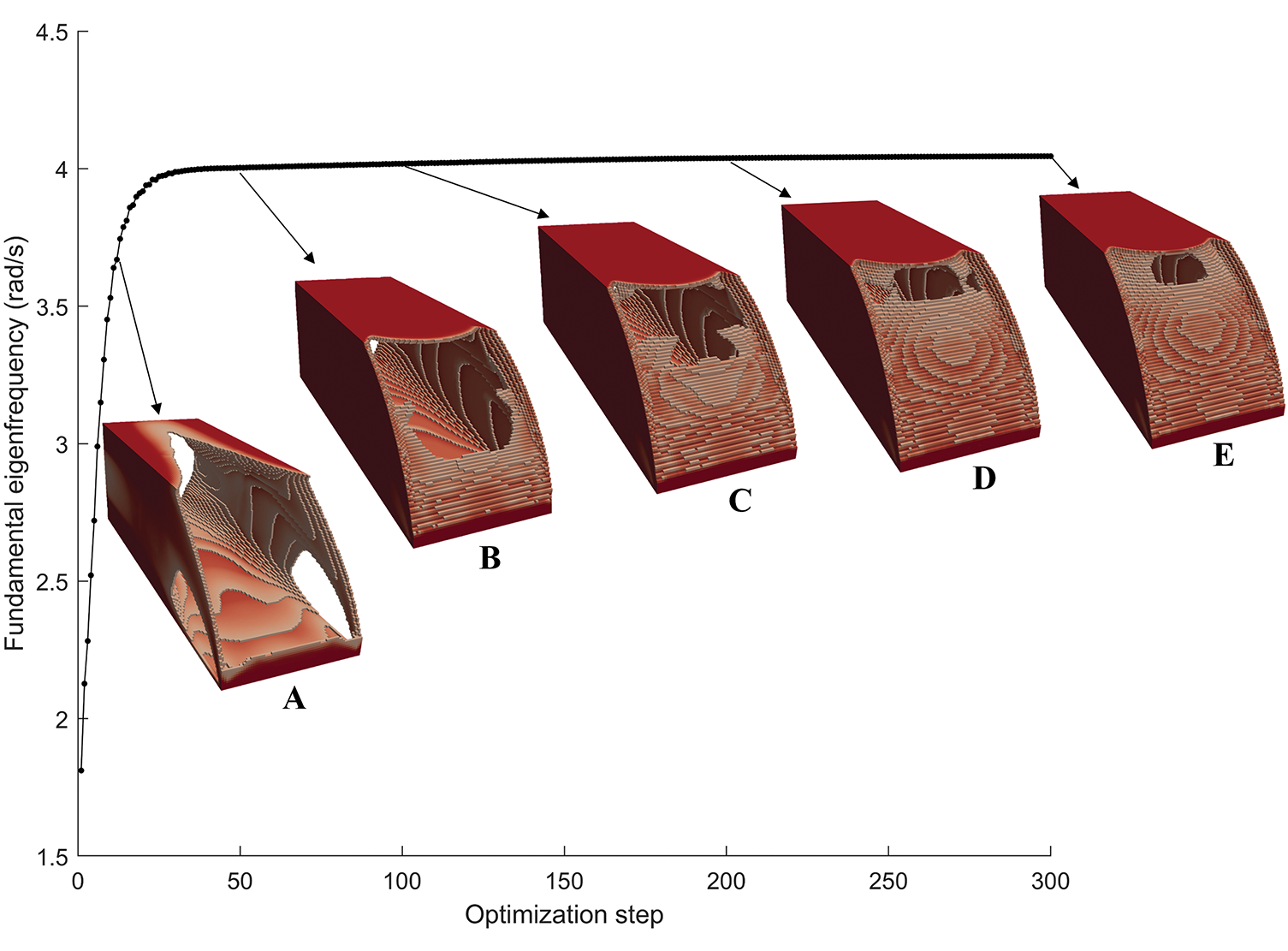
Figure 4: Iteration histories of fundamental eigenfrequency
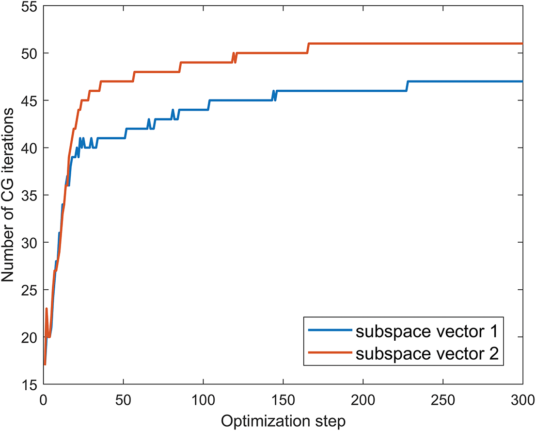
Figure 5: Iteration histories of the number of CG iterations
The fundamental eigenfrequency of the optimized design and the computation time are listed in Table 1. For comparison, those obtained by CPU-based SIAD and double-loop approaches [41] are also given. As given in [41], the CPU-based computation was performed on a workstation with dual Intel@ Xeon@ CPUs (E5-2670v3@2.3 GHz). It can be found that, though the maximum number of optimization steps is set to be three times of that in the CPU-based SIAD implementation [41], the computation time of the GPU-based SIAD implementation is only about
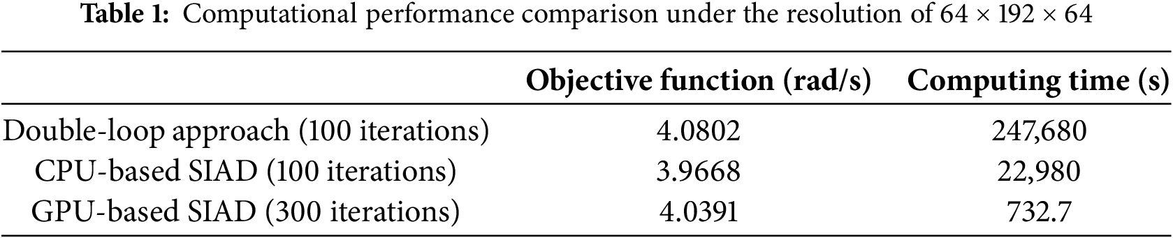
To demonstrate that the GPU solver works well for dealing with large-scale topology optimization problems, four resolutions are considered:
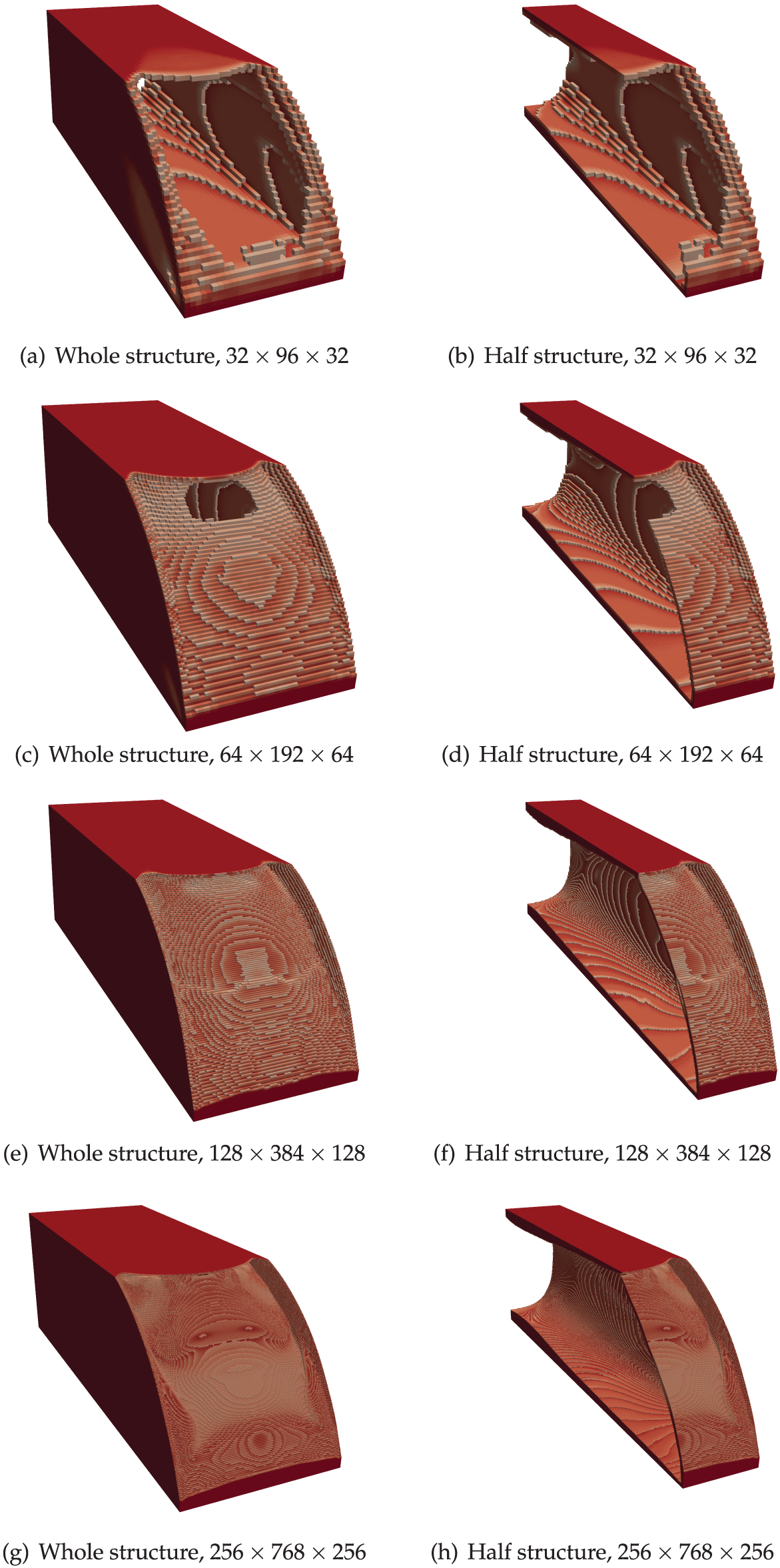
Figure 6: Optimized structure of the 3D cantilever beam using different resolutions for Case study 1
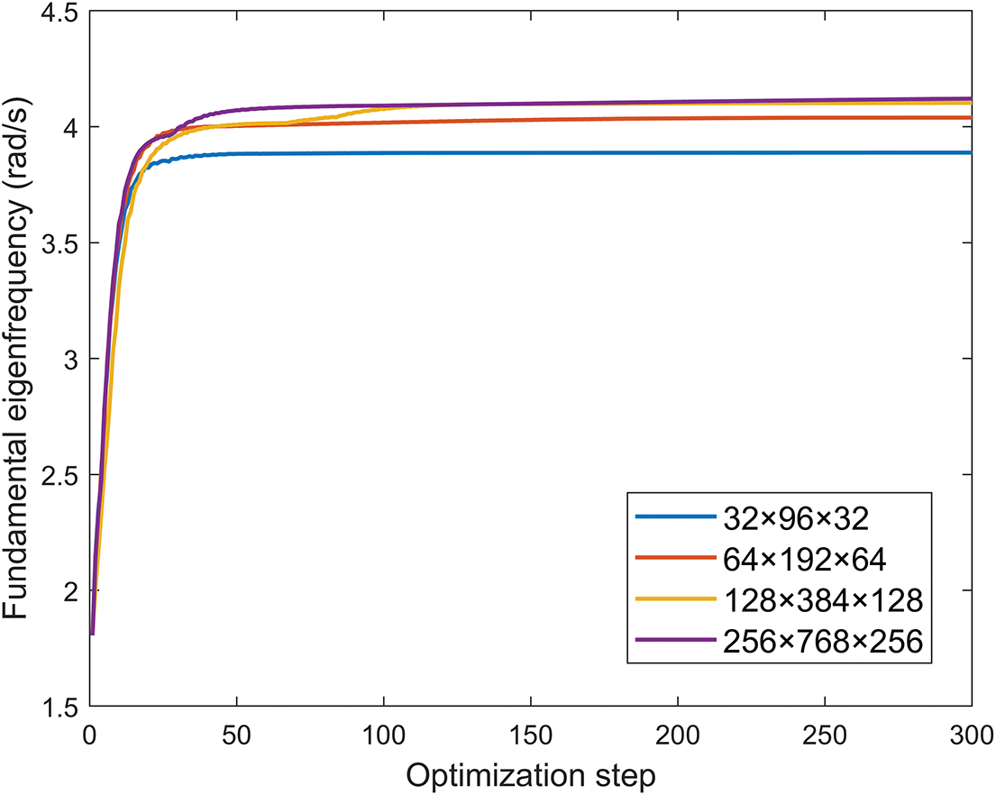
Figure 7: Iteration histories of different resolutions for Case study 1
The total computation times and their breakdowns for different resolutions are depicted in Figs. 8 and 9, respectively. It can be observed that the computation time corresponding to the finest mesh is approximately eight times that of the mesh with a resolution of
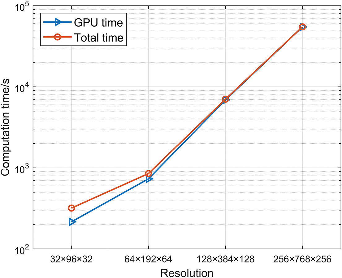
Figure 8: Computation times of different resolutions for Case study 1
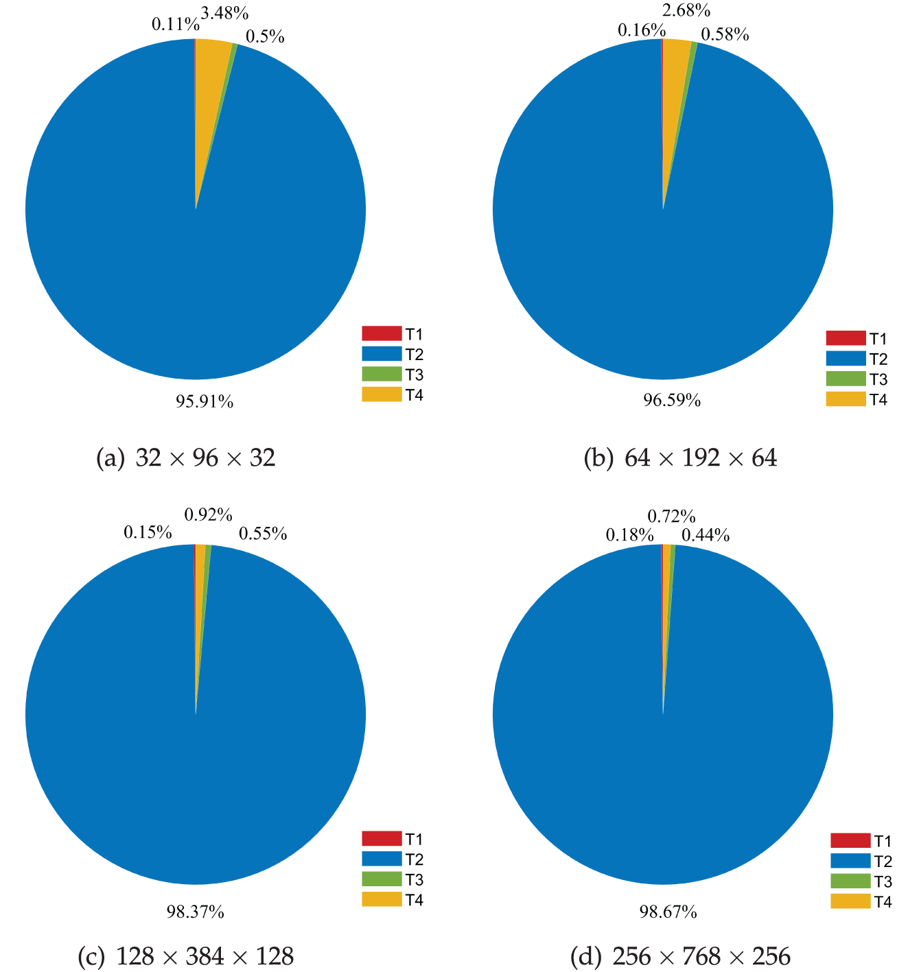
Figure 9: Breakdowns for total time of different resolutions for Case study 1
The original approximate fundamental eigenfrequency, the fundamental eigenfrequency re-analyzed using grid of the solution resolution and the finest resolution are shown in Fig. 10. Here, the eigenvalue solutions are obtained via the inverse iteration method, determining both eigenfrequencies and corresponding eigenmodes with a convergence criterion of
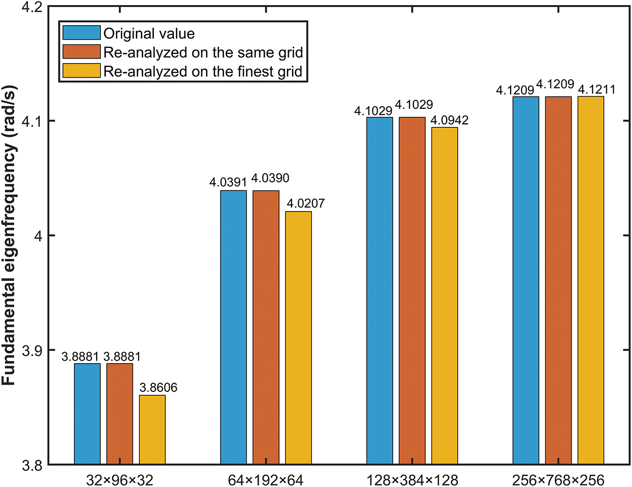
Figure 10: Fundamental eigenfrequencies obtained by re-analyzing the final designs on different grids
5.2 Case Study 2: Fundamental Eigenfrequency Maximization of a 3D Bracket Structure
The second example is to maximize the fundamental eigenfrequency of a simply-supported bracket structure, as shown in Fig. 11 with the green dashed lines indicating the enforced symmetry planes. The red circle at the center of the bottom surface with a diameter of 0.03125 m indicates the application region of the distributed nonstructural mass, with a total magnitude of 5000 kg. The design domain has dimensions of
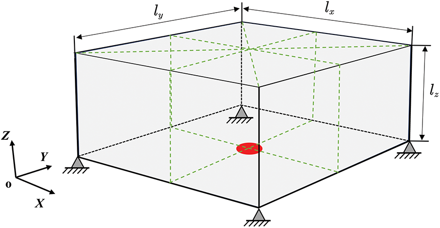
Figure 11: Definition of the 3D bracket structure design problem
The design domain is discretized into
The optimized structure is shown in Fig. 12. The iteration history of the first four lowest-order eigenfrequencies and some intermediate designs are plotted in Fig. 13, in which the threshold values of 0.3 (for solution A in the 10th optimization step), 0.6 (for solution B in the 100th optimization step) and 0.8 (for solution C and D in the 200th and the final optimization step, respectively) are set for the displayed density distribution. The fundamental eigenfrequency increased from 92.8729 to 358.2897 rad/s. It can be clearly observed that, except for the distinct eigenfrequencies corresponding to the initial guess eigenvectors, the first three eigenvalues in all other iteration steps are almost identical. This necessitates the special treatment of the repeated eigenvalues in the sensitivity analysis, as mentioned in Section 3. Similar to the first example, the optimized result is also re-analyzed on the same grid by the inverse iteration method. The obtained eigenfrequency, 358.2464 rad/s, is very close to the original optimized result, again demonstrating the convergence of the eigenvectors by the SIAD method. The total computation time for 300 iterations is 2494.6 s, and the breakdown is shown in Fig. 14. It can be seen that finite element analysis accounts for more than
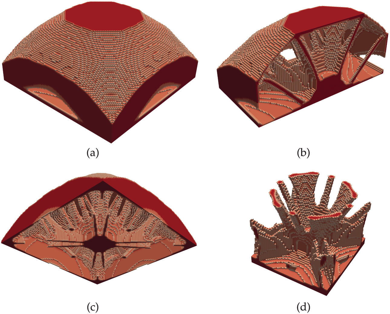
Figure 12: Optimized structure of the 3D bracket. (a) Whole structure; (b–d) view of different sections
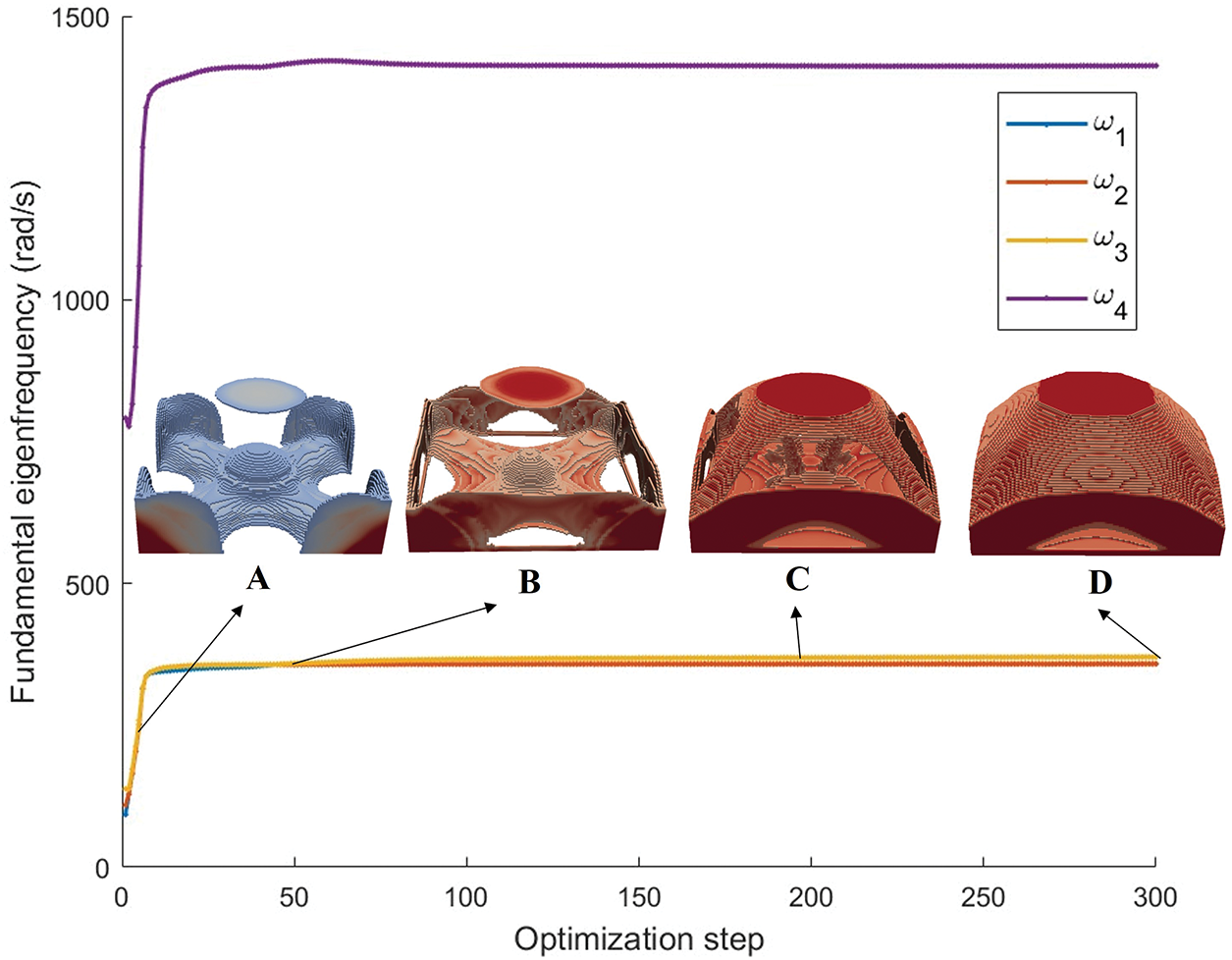
Figure 13: Iteration histories of objective functions for Case study 2
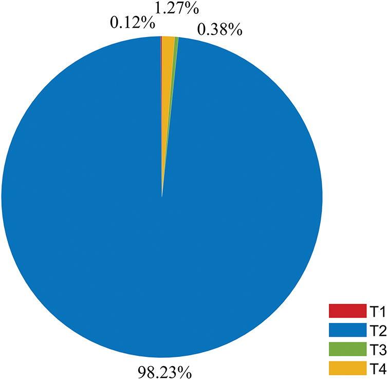
Figure 14: Breakdowns for total time of Case study 2
In this work, an efficient GPU solver is developed for maximizing fundamental eigenfrequency in large-scale 3D topology optimization. The computational cost of the original SIAD method is further reduced by using the GPU-based accelerated MGPCG method. The cluster-mean approach is adopted to address the non-differentiability issue caused by repeated eigenfrequencies. Numerical examples demonstrated the effectiveness of the SIAD method for topology optimization problems with high resolutions. Additionally, the ZPR algorithm is also proven to be efficient in design variable updating and works well with the SIAD method. This work achieved large-scale 3D topology optimization for maximizing the fundamental eigenfrequency with 50.33 million elements on a single GPU card for the first time, and the computation time is remarkably low at about 15.2 h for 300 iterations. Truss-like features are obtained for the coarse meshes, while variable-thickness, closed-walled structural characteristics with higher fundamental eigenfrequencies are generated for the fine meshes in the optimized topologies. The effectiveness of the proposed solver in the presence of repeated eigenfrequencies is also demonstrated.
While this work focuses on maximizing the fundamental eigenfrequency, many applications require maximizing higher-order eigenfrequencies or their gaps. In these situations, computing several eigenfrequencies is necessary, which incurs a higher computational cost than maximizing only the fundamental eigenfrequency. It should be noted that the proposed GPU solver can still be used to accelerate the finite element solution process in these cases, and a substantial reduction in computation time can be expected. However, solving these more complex problems would require bound formulations and other general constraints in addition to the volume fraction constraint. Consequently, the ZPR algorithm would be difficult to use for solving the sub-problem, making the MMA method necessary. In future work, we will parallelize the MMA method on GPUs to solve more general large-scale problems.
Acknowledgement: We are grateful to Professor Zhan Kang and Professor Xiaopeng Zhang from Dalian University of Technology for insightful discussions, valuable guidance, and constructive suggestions on this work. In developing this manuscript, DeepSeek R1 and Google Gemini were utilized as an English drafting aid. All AI-generated content underwent critical review and substantive editing by the authors, who maintain sole accountability for the final scholarly content.
Funding Statement: This work received support from the National Natural Science Foundation of China (Award No. 52105240).
Author Contributions: Conceptualization, Tianyuan Qi and Junpeng Zhao; Data curation, Tianyuan Qi; Formal analysis, Tianyuan Qi and Junpeng Zhao; Funding acquisition, Junpeng Zhao; Investigation, Tianyuan Qi; Methodology, Tianyuan Qi; Project administration, Junpeng Zhao and Chunjie Wang; Resources, Junpeng Zhao and Chunjie Wang; Software, Tianyuan Qi; Supervision, Junpeng Zhao; Validation, Tianyuan Qi and Junpeng Zhao; Visualization, Tianyuan Qi; Writing—original draft, Tianyuan Qi; Writing—review & editing, Junpeng Zhao and Chunjie Wang. All authors reviewed the results and approved the final version of the manuscript.
Availability of Data and Materials: All the data can be obtained from the corresponding author upon reasonable request.
Ethics Approval: Not applicable.
Conflicts of Interest: The authors declare no conflicts of interest to report regarding the present study.
References
1. Wijker JJ. Mechanical vibrations in spacecraft design. Cham, Switzerland: Springer Science & Business Media; 2013. [Google Scholar]
2. Wijker JJ. Spacecraft structures. Cham, Switzerland: Springer; 2008. [Google Scholar]
3. Fu J, Huang H, Chen S, Zhang Y, An H. A topology, material and beam section optimization method for complex structures. Eng Optimiz. 2025;57(6):1467–85. doi:10.1080/0305215x.2024.2357149. [Google Scholar] [CrossRef]
4. Zhu JH, Zhang WH, Xia L. Topology optimization in aircraft and aerospace structures design. Arch Comput Methods Eng. 2016;23(4):595–622. doi:10.1007/s11831-015-9151-2. [Google Scholar] [CrossRef]
5. Munk DJ, Miller JD. Topology optimization of aircraft components for increased sustainability. AIAA J. 2022;60(1):445–60. doi:10.2514/1.j060259. [Google Scholar] [CrossRef]
6. Chu S, Townsend S, Featherston C, Kim HA. Simultaneous layout and topology optimization of curved stiffened panels. AIAA J. 2021;59(7):2768–83. doi:10.2514/6.2020-3144. [Google Scholar] [CrossRef]
7. Manguri A, Magisano D, Jankowski R. Gradient-based weight minimization of nonlinear truss structures with displacement, stress, and stability constraints. Int J Numer Methods Eng. 2025;126(14):e70096. doi:10.1002/nme.70096. [Google Scholar] [CrossRef]
8. Bendsoe MP, Sigmund O. Topology optimization: theory, methods, and applications. Cham, Switzerland: Springer Science & Business Media; 2013. [Google Scholar]
9. Deaton JD, Grandhi RV. A survey of structural and multidisciplinary continuum topology optimization: post 2000. Struct Multidiscip Optim. 2014;49(1):1–38. doi:10.1007/s00158-013-0956-z. [Google Scholar] [CrossRef]
10. Manguri A, Hassan H, Saeed N, Jankowski R. Topology, size, and shape optimization in civil engineering structures: a review. Comput Model Eng Sci. 2025;142(2):933–71. doi:10.32604/cmes.2025.059249. [Google Scholar] [CrossRef]
11. Bendsøe MP, Kikuchi N. Generating optimal topologies in structural design using a homogenization method. Comput Methods Appl Mech Eng. 1988;71(2):197–224. doi:10.1016/0045-7825(88)90086-2. [Google Scholar] [CrossRef]
12. Bendsøe MP. Optimal shape design as a material distribution problem. Struct Optim. 1989;1(4):193–202. doi:10.1007/bf01650949. [Google Scholar] [CrossRef]
13. Zhou M, Rozvany GI. The COC algorithm, Part II: topological, geometrical and generalized shape optimization. Comput Methods Appl Mech Eng. 1991;89(1–3):309–36. doi:10.1016/0045-7825(91)90046-9. [Google Scholar] [CrossRef]
14. Wang MY, Wang X, Guo D. A level set method for structural topology optimization. Comput Methods Appl Mech Eng. 2003;192(1–2):227–46. doi:10.1016/s0045-7825(02)00559-5. [Google Scholar] [CrossRef]
15. Allaire G, Jouve F, Toader AM. Structural optimization using sensitivity analysis and a level-set method. J Comput Phys. 2004;194(1):363–93. doi:10.1016/j.jcp.2003.09.032. [Google Scholar] [CrossRef]
16. Xie YM, Steven GP. A simple evolutionary procedure for structural optimization. Comput Struct. 1993;49(5):885–96. [Google Scholar]
17. Huang X, Xie Y. Convergent and mesh-independent solutions for the bi-directional evolutionary structural optimization method. Finite Elem Anal Des. 2007;43(14):1039–49. doi:10.1016/j.finel.2007.06.006. [Google Scholar] [CrossRef]
18. Guo X, Zhang W, Zhong W. Doing topology optimization explicitly and geometrically—a new moving morphable components based framework. J Appl Mech. 2014;81(8):081009. doi:10.1115/1.4027609. [Google Scholar] [CrossRef]
19. Pedersen NL. Maximization of eigenvalues using topology optimization. Struct Multidiscip Optim. 2000;20(1):2–11. doi:10.1007/s001580050130. [Google Scholar] [CrossRef]
20. Olhoff N, Rasmussen SH. On single and bimodal optimum buckling loads of clamped columns. Int J Solids Struct. 1977;13(7):605–14. doi:10.1016/0020-7683(77)90043-9. [Google Scholar] [CrossRef]
21. Wang C, Zhang Y, Yu W, Yang S, Wang C, Jing S. Topology optimization of shell-infill structures for maximum stiffness and fundamental frequency. Compos Struct. 2025;356(10):118879. doi:10.1016/j.compstruct.2025.118879. [Google Scholar] [CrossRef]
22. Zhu Y, Wang Y, Zhang X, Kang Z. A new form of forbidden frequency band constraint for dynamic topology optimization. Struct Multidiscipl Optim. 2022;65(4):123. doi:10.1007/s00158-022-03220-1. [Google Scholar] [CrossRef]
23. Ma ZD, Kikuchi N, Cheng HC. Topological design for vibrating structures. Comput Methods Appl Mech Eng. 1995;121(1–4):259–80. doi:10.1016/0045-7825(94)00714-x. [Google Scholar] [CrossRef]
24. Kim TS, Kim YY. Mac-based mode-tracking in structural topology optimization. Comput Struct. 2000;74(3):375–83. [Google Scholar]
25. Tcherniak D. Topology optimization of resonating structures using SIMP method. Int J Numer Methods Eng. 2002;54(11):1605–22. doi:10.1002/nme.484. [Google Scholar] [CrossRef]
26. Du J, Olhoff N. Topological design of freely vibrating continuum structures for maximum values of simple and multiple eigenfrequencies and frequency gaps. Struct Multidiscip Optim. 2007;34(2):91–110. doi:10.1007/s00158-007-0101-y. [Google Scholar] [CrossRef]
27. Zhu J, Zhang W. Integrated layout design of supports and structures. Comput Methods Appl Mech Eng. 2010;199(9–12):557–69. doi:10.1016/j.cma.2009.10.011. [Google Scholar] [CrossRef]
28. Niu B, Yan J, Cheng G. Optimum structure with homogeneous optimum cellular material for maximum fundamental frequency. Struct Multidiscip Optim. 2009;39(2):115–32. doi:10.1007/s00158-008-0334-4. [Google Scholar] [CrossRef]
29. Yan X, Xu Q, Hua H, Huang W, Huang X. Concurrent optimization of macrostructures and material microstructures and orientations for maximizing natural frequency. Eng Struct. 2020;209(2):109997. doi:10.1016/j.engstruct.2019.109997. [Google Scholar] [CrossRef]
30. Seyranian AP, Lund E, Olhoff N. Multiple eigenvalues in structural optimization problems. Struct Optim. 1994;8(4):207–27. doi:10.1007/bf01742705. [Google Scholar] [CrossRef]
31. Xia Q, Shi T, Wang MY. A level set based shape and topology optimization method for maximizing the simple or repeated first eigenvalue of structure vibration. Struct Multidiscip Optim. 2011;43(4):473–85. doi:10.1007/s00158-010-0595-6. [Google Scholar] [CrossRef]
32. Deng Z, Liang Y, Cheng G. Discrete variable topology optimization for maximizing single/multiple natural frequencies and frequency gaps considering the topological constraint. Int J Numer Methods Eng. 2024;125(10):e7449. doi:10.1002/nme.7449. [Google Scholar] [CrossRef]
33. Leader MK, Chin TW, Kennedy GJ. High-resolution topology optimization with stress and natural frequency constraints. AIAA J. 2019;57(8):3562–78. doi:10.2514/1.j057777. [Google Scholar] [CrossRef]
34. Ferrari F, Sigmund O. Revisiting topology optimization with buckling constraints. Struct Multidiscip Optim. 2019;59(5):1401–15. doi:10.1007/s00158-019-02253-3. [Google Scholar] [CrossRef]
35. Zhang G, Khandelwal K, Guo T. Topology optimization of stability-constrained structures with simple/multiple eigenvalues. Int J Numer Methods Eng. 2024;125(3):e7387. doi:10.1002/nme.7387. [Google Scholar] [CrossRef]
36. Sun S, Khandelwal K. A cluster mean approach for topology optimization of natural frequencies and bandgaps with simple/multiple eigenfrequencies. arXiv:2501.14910. 2025. [Google Scholar]
37. Zhou P, Du J, Lü Z. Topology optimization of freely vibrating continuum structures based on nonsmooth optimization. Struct Multidiscip Optim. 2017;56(3):603–18. doi:10.1007/s00158-017-1677-5. [Google Scholar] [CrossRef]
38. Ferrari F, Lazarov BS, Sigmund O. Eigenvalue topology optimization via efficient multilevel solution of the frequency response. Int J Numer Methods Eng. 2018;115(7):872–92. doi:10.1002/nme.5829. [Google Scholar] [CrossRef]
39. Andreassen E, Ferrari F, Sigmund O, Diaz AR. Frequency response as a surrogate eigenvalue problem in topology optimization. Int J Numer Methods Eng. 2018;113(8):1214–29. doi:10.1002/nme.5563. [Google Scholar] [CrossRef]
40. Fu Y, Kennedy GJ. Quasi-Newton corrections for compliance and natural frequency topology optimization problems. Struct Multidiscipl Optim. 2023;66(8):176. doi:10.1007/s00158-023-03630-9. [Google Scholar] [CrossRef]
41. Kang Z, He J, Shi L, Miao Z. A method using successive iteration of analysis and design for large-scale topology optimization considering eigenfrequencies. Comput Methods Appl Mech Eng. 2020;362:112847. doi:10.1016/j.cma.2020.112847. [Google Scholar] [CrossRef]
42. Cheng G, Xu L, Jiang L. A sequential approximate programming strategy for reliability-based structural optimization. Comput Struct. 2006;84(21):1353–67. [Google Scholar]
43. Shi L, Li J, Liu P, Zhu Y, Kang Z. A multi-step relay implementation of the successive iteration of analysis and design method for large-scale natural frequency-related topology optimization. Comput Mech. 2024;73(2):403–18. doi:10.1007/s00466-023-02372-1. [Google Scholar] [CrossRef]
44. Wadbro E, Berggren M. Megapixel topology optimization on a graphics processing unit. SIAM Rev. 2009;51(4):707–21. doi:10.1137/070699822. [Google Scholar] [CrossRef]
45. Schmidt S, Schulz V. A 2589 line topology optimization code written for the graphics card. Compute Vis Sci. 2011;14(6):249–56. doi:10.1007/s00791-012-0180-1. [Google Scholar] [CrossRef]
46. Träff EA, Rydahl A, Karlsson S, Sigmund O, Aage N. Simple and efficient GPU accelerated topology optimisation: codes and applications. Comput Methods Appl Mech Eng. 2023;410(6):116043. doi:10.1016/j.cma.2023.116043. [Google Scholar] [CrossRef]
47. Zhang D, Zhai X, Liu L, Fu XM. An optimized, easy-to-use, open-source GPU solver for large-scale inverse homogenization problems. Struct Multidiscipl Optim. 2023;66(9):207. doi:10.1007/s00158-023-03657-y. [Google Scholar] [CrossRef]
48. Zhao J, Qi T, Wang C. Efficient GPU accelerated topology optimization of composite structures with spatially varying fiber orientations. Comput Methods Appl Mech Eng. 2024;421(1):116809. doi:10.1016/j.cma.2024.116809. [Google Scholar] [CrossRef]
49. Qi T, Zhao J, Wang C. An efficient GPU solver for 3D topology optimization of continuous fiber-reinforced composite structures. Comput Methods Appl Mech Eng. 2025;435(6):117675. doi:10.1016/j.cma.2024.117675. [Google Scholar] [CrossRef]
50. Wu J, Dick C, Westermann R. A system for high-resolution topology optimization. IEEE Trans Vis Comput Graph. 2015;22(3):1195–208. doi:10.1109/tvcg.2015.2502588. [Google Scholar] [PubMed] [CrossRef]
51. Zhang D, Zhai X, Fu XM, Wang H, Liu L. Wiley online library. Large-scale worst-case topology optimization. Comput Graph Forum. 2022;41(7):529–40. [Google Scholar]
52. Bourdin B. Filters in topology optimization. Int J Numer Methods Eng. 2001;50(9):2143–58. doi:10.1002/nme.116. [Google Scholar] [CrossRef]
53. Stolpe M, Svanberg K. An alternative interpolation scheme for minimum compliance topology optimization. Struct Multidiscip Optim. 2001;22(2):116–24. doi:10.1007/s001580100129. [Google Scholar] [CrossRef]
54. Bathe KJ, Ramaswamy S. An accelerated subspace iteration method. Comput Methods Appl Mech Eng. 1980;23(3):313–31. doi:10.1016/0045-7825(80)90012-2. [Google Scholar] [CrossRef]
55. Dick C, Georgii J, Westermann R. A real-time multigrid finite hexahedra method for elasticity simulation using CUDA. Simul Model Pract Th. 2011;19(2):801–16. doi:10.1016/j.simpat.2010.11.005. [Google Scholar] [CrossRef]
56. Aage N, Lazarov BS. Parallel framework for topology optimization using the method of moving asymptotes. Struct Multidiscip Optim. 2013;47(4):493–505. doi:10.1007/s00158-012-0869-2. [Google Scholar] [CrossRef]
57. Zhang XS, Paulino GH, Ramos ASJr. Multi-material topology optimization with multiple volume constraints: a general approach applied to ground structures with material nonlinearity. Struct Multidiscip Optim. 2018;57(1):161–82. doi:10.1007/s00158-017-1768-3. [Google Scholar] [CrossRef]
58. Giraldo-Londono O, Paulino GH. PolyDyna: a Matlab implementation for topology optimization of structures subjected to dynamic loads. Struct Multidiscip Optim. 2021;64(2):957–90. doi:10.1007/s00158-021-02859-6. [Google Scholar] [CrossRef]
59. Hu Y, Li TM, Anderson L, Ragan-Kelley J, Durand F. Taichi: a language for high-performance computation on spatially sparse data structures. ACM Trans Graph (TOG). 2019;38(6):1–16. [Google Scholar]
60. Ayachit U. The paraview guide: a parallel visualization application. Clifton Park, NY, USA: Kitware, Inc.; 2015. [Google Scholar]
61. Sigmund O, Aage N, Andreassen E. On the (non-)optimality of Michell structures. Struct Multidiscip Optim. 2016;54(2):361–73. doi:10.1007/s00158-016-1420-7. [Google Scholar] [CrossRef]
62. Liu H, Hu Y, Zhu B, Matusik W, Sifakis E. Narrow-band topology optimization on a sparsely populated grid. ACM Trans Graph (TOG). 2018;37(6):1–14. doi:10.1145/3272127.3275012. [Google Scholar] [CrossRef]
Cite This Article
 Copyright © 2025 The Author(s). Published by Tech Science Press.
This work is licensed under a Creative Commons Attribution 4.0 International License , which permits unrestricted use, distribution, and reproduction in any medium, provided the original work is properly cited.
 Downloads
 Citation Tools