A CGAN Framework for Predicting Crack Patterns and Stress-Strain Behavior in Concrete Random Media

1  Introduction

Quasi-brittle materials such as concrete, ceramics, and rocks demonstrate distinct mechanical behavior governed by inherent microstructural heterogeneity. Unlike homogeneous systems, where crack propagation follows deterministic fracture mechanics principles, these random media exhibit stochastic fracture patterns influenced by localized variations in material strength, porosity, and fracture energy dissipation [1]. The random nature of crack initiation and growth in such heterogeneous systems creates significant challenges for the precise prediction of fracture propagation trajectories and associated mechanical performance degradation. This stochastic fracture behavior necessitates advanced computational frameworks capable of resolving microstructural variability effects on macroscale failure processes.

The Finite Element Method (FEM) is a widely recognized tool for simulating the fracture behavior of random media, which are characterized by randomness due to their heterogeneous microstructures. Effectively modeling the stochastic nature is essential for understanding crack propagation and predicting structural performance under various loading conditions. Among the approaches developed, random field modeling has proven to be a practical and reliable method that captures spatial heterogeneity and provides a realistic foundation for crack simulations. Xu and Graham-Brady [2] developed a stochastic framework for analyzing elastic media. Koutsourelakis and Deodatis [3] presented methods for simulating binary random fields in two-phase materials. Ren and Li [4,5] explored concrete cracking processes by using random field modeling and the Cohesive Zone Model (CZM), which simulates nonlinear mechanical behavior by explicitly defining traction-separation laws [6]. Subsequently, Wu et al. [7] and Zhang et al. [8] applied random field modeling in conjunction with phase-field methods to investigate probabilistic fractures in quasi-brittle materials. Wu et al. [9] employed random field modeling and a Convolutional Neural Network (CNN) to predict multiscale damage responses of random materials. The development and combination of such sophisticated fracture models are central to these simulations. For instance, a hybrid cohesive phase-field method has been recently developed to analyze the stability of complex rock slopes with discontinuities [10]. The scope of random field modeling has since expanded to include composite materials, such as FRP-reinforced concrete [11,12] and UHPC [13]. Its applications now encompass structural analyses, ranging from the bending failure of reinforced concrete beams [14] to the compression-bending failure of columns [15]. These advancements not only enhance the accuracy and reliability of crack predictions but also deepen our understanding of material behavior under stochastic conditions. While these advancements enhance prediction accuracy, such FEM-based methods are computationally intensive. Simulating crack propagation for hundreds or thousands of random samples, often required for robust MC Simulations in stochastic fracture, can take days or weeks [16]. These high computational demands limit the flexibility in exploring a wide range of loading conditions and material configurations for real-time engineering applications [17,18].

In recent years, deep learning methods have drawn attention for their ability to identify complex patterns directly from datasets. These models are highly effective in detecting and predicting crack patterns in quasi-brittle materials like concrete. Methods, including structural damage type identification via ensemble learning algorithms based on a Deep Convolutional Neural Network (DCNN) [19], a U-shaped Convolutional Neural Network (UNet)-based architecture enhanced with attention mechanisms, dilated convolutions, and depth-wise separable residual modules is proposed to improve the accuracy of boundary and detail recognition in pavement crack detection [20], and crack type classification using a multi-stage You Only Look Once-Vision Transformer (YOLO-ViT) model [21] have demonstrated their potential in this field. Generative Adversarial Networks (GANs) stand out among deep learning techniques due to their ability to generate high-quality and diverse images. By adopting the dynamic interplay between a generator and a discriminator, GAN not only improve unsupervised learning capabilities but also enhance feature extraction and data augmentation. Recent applications include cementitious composites crack detection and growth prediction based on residual pyramidal GAN [22], forecasting road surface cracks using Forecasted Crack Generative Adversarial Network (FC-GAN) [23], and prediction of discontinuous crack paths in random porous media via a Conditional Generative Adversarial Network (CGAN) [24]. Recent sophisticated applications also include using deep learning to detect crack damage in shield tunnels, which then informs a subsequent mesoscale cohesive numerical model to investigate the mechanical behavior [25]. Some deep learning models have also begun to explore the combined prediction of crack patterns and mechanical responses [26]. However, these existing models often do not holistically predict both stochastic crack patterns and their corresponding stress-strain behavior, driven by the inherent spatial variability of material properties in quasi-brittle materials like concrete. Furthermore, their application as efficient surrogate models for extensive large-scale stochastic analyses remains less explored. Therefore, a clear need exists for models that can comprehensively predict crack patterns under loading while accurately capturing the stochastic nature of heterogeneous materials and their full mechanical response.

To address these challenges, this study proposes an approach combining CGAN with random field modeling. Random field modeling captures the randomness of material properties, while FEM simulations generate crack propagation data and stress-strain curves data to train the CGAN. This model successfully predicts both stochastic crack patterns and stress-strain curves, demonstrating its capability in capturing key material behaviors. The trained model is then utilized as a surrogate model to perform extensive statistical analyses for crack density, spatial distribution, and other stochastic characteristics. The flowchart of this study is illustrated in Fig. 1. Compared to traditional FEM-based methods, this approach drastically reduces computational costs while maintaining robust predictive capabilities. By addressing the randomness and complexity inherent in quasi-brittle materials, the proposed method offers a practical tool for large-scale analysis and crack behavior predictions.

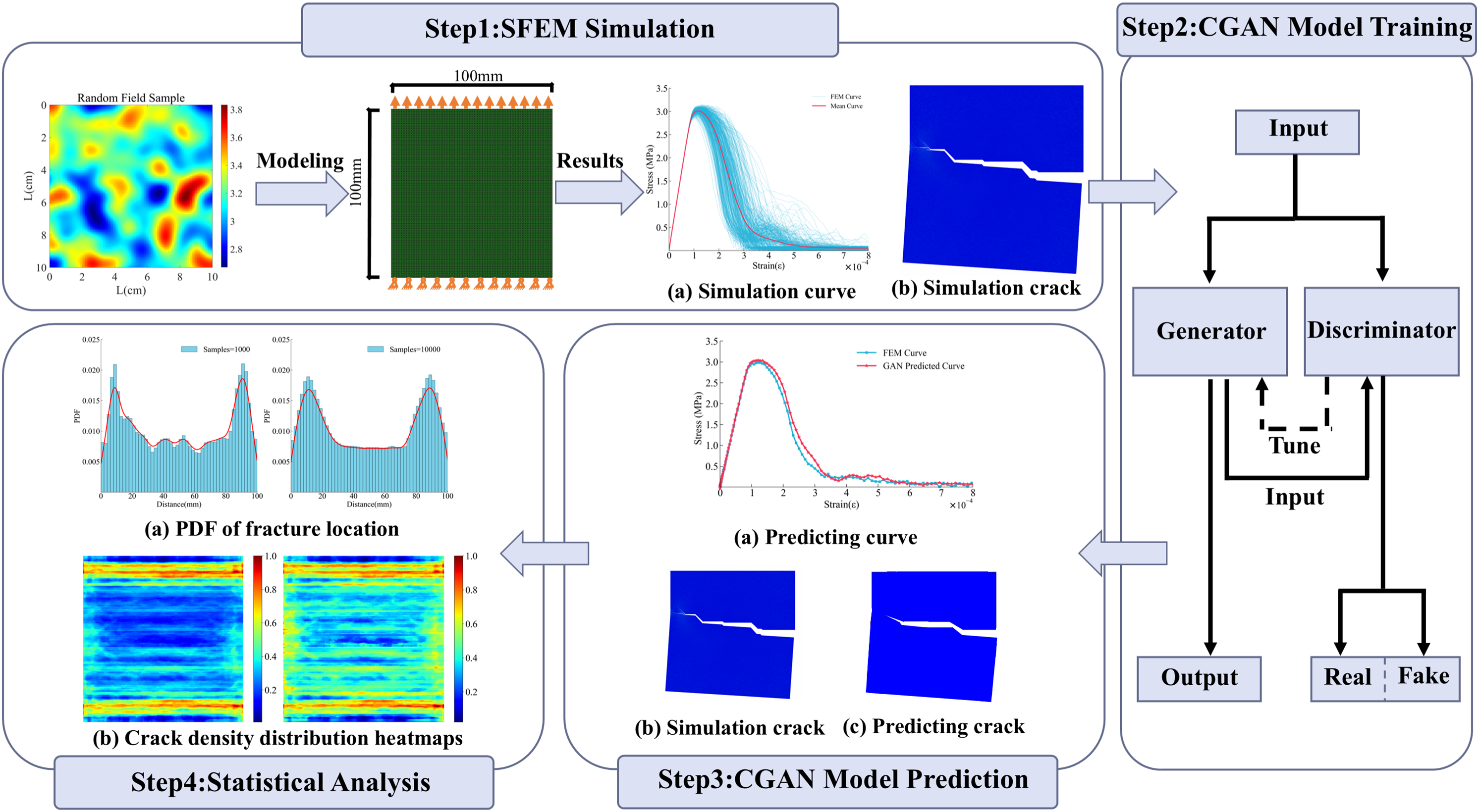
Figure 1: Research process flowchart

2  Background of Fracture Analysis of Random Media

2.1 Random Field Model for Random Media

To capture the randomness of random media, this study utilizes random field modeling. In this study, the spectral representation method [27] is adopted, which is a structurally precise method for discretizing random field parameters. Owing to its simulation performance, the spectral representation method has been widely adopted in various engineering random field simulations, which provides a powerful tool for understanding the spatial distribution laws of material properties [28].

In this research, the spatial distribution of the 2D random field Z(x,y) can be described as:

Z(x,y)=μft+σftZ0(x,y)(1)

where μft represents the average value of concrete tensile strength obtained from experimental statistics. σft denotes the standard deviation of the tensile strength field; Z0(x,y) is the standardized random field with zero mean and unit variance.

To generate a random field, it is essential to define the autocorrelation function, which is generally expressed as:

Rf0f0(ξ,η)=E[f0(x1,y1)f0(x2,y2)](2)

where ξ=x1−x2 and η=y1−y2 represent the separation distances in the x and y directions, respectively; E[⋅] denotes the expectation operator.

The autocorrelation function is related to the Power Spectral Density (PSD) function Sf0f0 through the Fourier transform as:

Sf0f0(κ1,κ2)=1(2π)2∫−∞∞∫−∞∞Rf0f0(ξ,η)e−i(κ1ξ+κ2η)dξdη(3)

where κ1 and κ2 are the wave numbers along x and y directions.

The standardized random field, with a zero mean and unit variance, can be obtained as follows:

Z0(x,y)=∑n1=1N1∑n2=1N2[An1n2cos⁡(κ1n1x+κ2n2y+Φn1n21)++A~n1n2cos⁡(κ1n1x−κ2n2y+Φn1n22)](4)

where Φn1n21 and Φn1n22 are the random phase angles uniformly distributed in the interval [0, 2π).

Based on the Eq. (3), the amplitudes corresponding to each wave number component in the random field can be calculated:

An1n2=2Sf0f0(κ1n1,κ2n2)Δκ1Δκ2(5)

A~n1n2=2Sf0f0(κ1n1,−κ2n2)Δκ1Δκ2(6)

κ1n1=n1Δκ1;κ2n2=n2Δκ2(7)

Δκ1=κ1uN1;Δκ2=κ2uN2(8)

where An1n2 and A~n1n2 represent the amplitudes along the x and y directions, respectively, which can be calculated based on the PSD function Sf0f0; κ1n1 and κ2n2 correspond to the specific wave number components at the n1-th and n2-th wave points along the x and y directions, respectively; κ1u and κ2u denote the cut-off wave numbers in the x and y directions; Δκ1 and Δκ2 represent the wave number discretization intervals; N1 and N2 represent the total number of wave components.

2.2 Simulation of Fracture

The CZM [29] provides a framework for analyzing crack propagation and failure mechanisms in brittle or quasi-brittle materials. It describes a nonlinear relationship between interfacial stress and crack opening displacement. Cracks initiate when the displacement exceeds the critical cohesive strength and then propagate progressively.

Within this context, our numerical modeling of random media employs a bilinear CZM formulation to describe interface failure through two sequential phases: an initial elastic loading stage with linear stress accumulation up to peak strength, succeeded by a material-softening stage culminating in complete fracture. The governing equations for this bilinear behavior are expressed as:

tn={σmaxδn0⋅δn,ifδn≤δn0,σmax(1−δn−δn0δnf−δn0),if δn0<δn≤δnf,0,ifδn>δnf.(9)

where tn represents the normal stress at the interface; δn is the interface displacement; σmax is the peak interface stress; δn0 is the displacement at peak stress; δnf is the displacement at the fracture point.

During the loading process, the normal stress tn increases linearly with the interface displacement δn, describing the elastic deformation behavior of the material. Once the displacement exceeds δn0, the material enters the softening phase, and the normal stress tn decreases linearly with displacement δn. When the displacement exceeds δnf, the interface stress tn becomes zero, which means the material interface has completely failed.

3  CGAN-Based Prediction of Material Mechanical Behavior

GAN is a deep learning framework designed for generating realistic data through an adversarial process between two neural networks: a generator and a discriminator [30]. The generator learns to produce synthetic data samples that resemble real data, while the discriminator evaluates the authenticity of these samples. A key variant is the CGAN [31], which enables controlled data generation through conditional inputs. In this study, CGAN is utilized to predict crack patterns and stress-strain curves in random media.

3.1 The Basic Principles of CGAN

In the traditional GAN framework, the generator maps noise vectors into data samples that resemble real ones through a series of nonlinear transformations. The discriminator then determines whether these samples are real or generated, as shown in Fig. 2. Since the input is purely random, the generator can produce diverse samples.

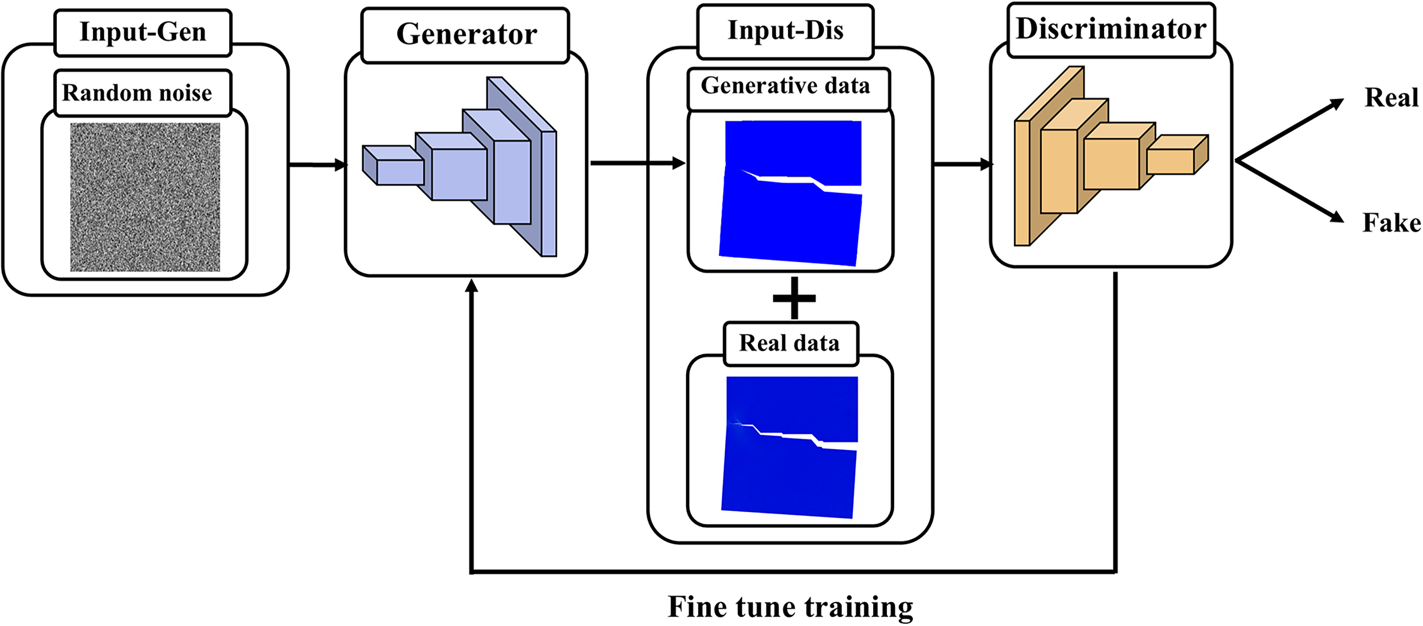
Figure 2: The basic structure of GAN

The objective function of a GAN balances the adversarial losses between the generator and the discriminator. The generator aims to produce realistic data, while the discriminator works to distinguish between real and generated data. The objective function can be established as:

minGmaxDV(D,G)=EX∼pdata(X)[log⁡D(X)]+Ez∼pz(z)[log⁡(1−D(G(z)))](10)

where G represents the generator; D represents the discriminator; EX∼pdata(X)[log⁡D(X)] represents the expected value of the logarithm of the probability that the discriminator classifies real data samples as real. Ez∼pz(z)[log⁡(1−D(G(z)))] represents the expected value of the logarithm of the probability that the discriminator classifies generated data samples as fake; X∼pdata(X) denotes samples drawn from the real data distribution; z∼pz(z) represents random noise drawn from a noise distribution; G(z) is the sample generated by the generator from the noise.

To address the lack of control in traditional GAN during data generation, CGAN is introduced. By incorporating conditional information into both the generator and the discriminator, CGAN guides the generation process under specific constraints, as illustrated in Fig. 3.

Figure 3: The structure of CGAN with conditional input

The generator not only aims to produce realistic samples but also ensures they are consistent with the given conditions. Meanwhile, the discriminator evaluates both the authenticity and the correctness of the condition-sample pair. The objective function is defined as [31]:

minGmaxDV(D,G)=EX∼pdata(X)[log⁡D(X|c)]+Ez∼pz(z)[log⁡(1−D(G(z|c)|c))](11)

where c represents the conditional information; G(z|c) is the sample generated by the generator based on noise z and conditional information c; D(X|c) represents the probability that the discriminator judges a real data sample as genuine based on the conditional information c.

3.2 CGAN-Based Prediction of Crack Path

Instead of explicitly encoding physical crack propagation criteria, the CGAN operates as a data-driven model. It learns from a large dataset of FEM-generated data, consisting of input random field images and their corresponding output crack patterns. This learning process allows it to implicitly extract the complex patterns and rules governing crack initiation and propagation.

3.2.1 The Structure of Generator

In this study, the generator adopts a deep convolutional neural network based on the Residual Network (ResNet) architecture to effectively extract and utilize deep features from the input images. ResNet [32] is a variant of CNN that introduces residual blocks to alleviate the problems of vanishing gradients and training degradation caused by increasing network depth.

As shown in Fig. 4, we optimize and modify the ResNet architecture. The main modifications include removing the fully connected layers from the original architecture, adding a series of transposed convolution layers, and introducing a Sigmoid activation function. These changes allow the network to gradually upsample the feature maps, generating images that correspond to the input conditions.

Figure 4: The hierarchical structure of the ResNet

The generator retains the core ResNet architecture, including residual blocks with skip connections, which effectively handle detail-rich crack images. Initial feature extraction is performed using a 7 × 7 convolutional kernel with batch normalization and ReLU activation. The generator then stacks bottleneck residual blocks with 1 × 1, 3 × 3, and 1 × 1 convolutional layers to progressively enhance image features. Finally, transposed convolution layers restore spatial resolution by expanding the feature map, as shown in Fig. 5.

Figure 5: Illustration of transposed convolution

In the transposed convolution operation, the kernel traverses the feature map with a specified stride, performing weighted multiplication and accumulation at each position. This process can be precisely defined by the following equation [32]:

Y=λ∗w+b(12)

where λ represents the input feature tensor; w denotes the transposed convolution kernel weights; b is the bias term.

Each transposed convolution layer is followed by batch normalization and a ReLU activation. This design improves stability and preserves feature representation during upsampling. Finally, the generator uses the Sigmoid function to restrict the pixel values of the output image to the range [0, 1]. The formula for the Sigmoid function is given as follows:

fSigmoid(λ)=11+e−λ(13)

3.2.2 The Structure of Discriminator

In this study, the discriminator adopts the PatchGAN architecture. PatchGAN is a fully convolutional neural network [33], and its architecture primarily consists of an input layer and a series of down sampling modules, as illustrated in Fig. 6. The core idea is to assess the authenticity of an image in a localized manner by dividing the input image into multiple smaller patches and then judging each patch individually.

Figure 6: The hierarchical structure of the PatchGAN

In the PatchGAN workflow, input images are progressively downsampled through modules consisting of convolutional layers, Leaky ReLU activation functions, and normalization layers. Leaky ReLU prevents gradient vanishing by allowing a small gradient flow for negative input values, ensuring stable training [34]. The calculation formula is represented as [35]:

fLeakyReLU(λ)={λ,if λ>0αλ,if λ≤0(14)

where α is a small positive constant that controls the slope in the negative region.

By evaluating each patch individually, PatchGAN effectively captures both local characteristics and global consistency, demonstrating superior performance in complex crack generation tasks. Additionally, this local discrimination approach reduces the number of parameters and computational complexity, thereby enhancing the efficiency of model training.

3.3 CGAN-Based Prediction of Stress-Strain Curve

To comprehensively analyze the failure mechanisms of random media, this study introduces stress-strain curve prediction as a complementary perspective alongside crack prediction. A CGAN-based deep learning model is constructed to predict the stress-strain curves of random media under specific loading conditions. The model architecture is specifically optimized to align with the unique properties of stress-strain data.

To better model stress-strain curves, the generator removes transpose convolutions and adopts fully connected layers to capture global relationships. The discriminator uses one-dimensional convolutional layers to extract curve features, which are concatenated with random field image features for joint evaluation. The overall architecture is shown in Fig. 7.

Figure 7: The hierarchical structure of the model for curve prediction. (a) Generator for curve prediction; (b) Discriminator for curve prediction

4  Results and Discussion

This study investigates the tensile cracking behavior of random media using concrete as a case study. A random field model is employed to characterize the spatial variability of material properties, and FEM simulations are conducted to generate corresponding crack images and stress-strain curves. A CGAN model is developed to predict crack propagation and stress–strain behavior. This enables accurate reconstruction of fracture processes. In addition, the CGAN serves as a surrogate model for large-sample analysis. It facilitates efficient statistical evaluation of crack distribution and density.

4.1 Random Field Representation for Concrete

Concrete is a typical random medium that exhibits complex constituents that significantly influence its cracking behavior. The random distribution of material properties, such as tensile strength and fracture energy, plays a key role in the initiation and propagation of cracks. According to the research by Guan et al. [36], the tensile strength of concrete in this study is modeled as a homogeneous random field parameter to capture the randomness in material properties.

To generate the random field samples essential for this study, a Gaussian autocorrelation function is adopted to characterize the spatial correlation of material properties. From this autocorrelation function, the corresponding PSD function is derived, with its mathematical formulations provided in Eqs. (15) and (16).

Rf0f0(ξ,η)=σ2exp⁡[−(ξ2+η2L2)](15)

Sf0f0(κ1,κ2)=σ2L24πexp⁡[−(L2κ12+L2κ224)](16)

where L is the correlation length of the random field.

The distribution range of tensile strength is defined with a mean value μft=3.2MPa and a standard deviation σft=0.2MPa. Based on the research by Bazant and Pijaudier-Cabot [37], the correlation length for concrete is generally taken as the maximum aggregate size. Referring to the experimental data from Ren et al. [38], the correlation length is chosen to be the maximum aggregate size of concrete (8 mm). Referencing Shinozuka’s research [27], the optimal cut-off wave number is determined to be 5 rad/mm. The key parameters determined are summarized in Table 1.

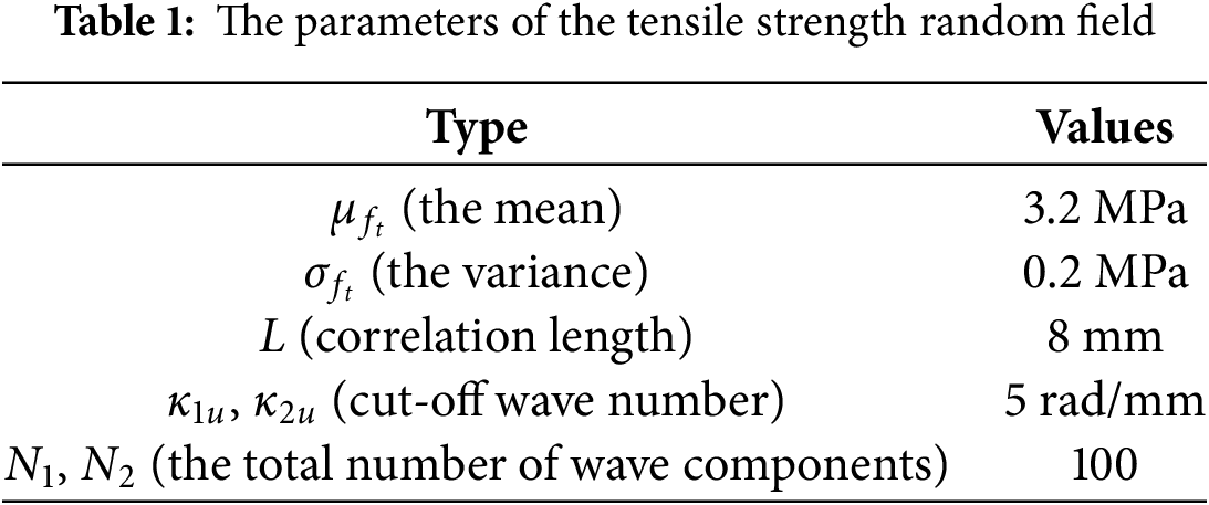
Random field samples of tensile strength are generated based on the parameters in Table 1, as shown in Fig. 8.

Figure 8: Random field samples. (a) Sample 1; (b) Sample 2

4.2 FEM Simulations

The FEM simulation integrates both the random field model and the CZM to simulate crack patterns and stress-strain behavior in concrete under uniaxial tension, as shown in Fig. 9.

Figure 9: Finite element model and boundary conditions

First, triangular elements are used to discretize the concrete specimen. A CZM simulates the nonlinear mechanical behavior, with material parameters as: Young’s modulus of 37,000 MPa, Poisson’s ratio of 0.2. and fracture energy of 0.1 N/mm, selected based on established experimental results for concrete from the literature [39,40]. Zero-thickness, four-node cohesive elements (COH2D4) [41] are inserted into the mesh via a custom Python script to model crack initiation and propagation, as shown in Fig. 9. The specimen is simply supported at the bottom and subjected to a monotonically increasing total displacement u of 6 mm at the top. This displacement magnitude is selected to ensure sufficient crack propagation, thereby enhancing the visual clarity of crack patterns. Under these conditions, crack images and stress-strain curves are obtained. Post-processing is then performed to extract the corresponding data for training the deep learning model. A dataset of 500 samples, including crack propagation images and corresponding stress-strain curves, is generated through FEM under uniaxial tensile loading, as shown in Fig. 10.

Figure 10: Uniaxial tensile sample crack. (a) Sample 1; (b) Sample 2

The crack images reveal different fracture patterns under tensile loading, underscoring the role of material heterogeneity in governing crack initiation and propagation paths. Correspondingly, the stress–strain curves exhibit substantial dispersion in the descending segment, as shown in Fig. 11. These findings confirm that combining the random field model with the CZM is effective. The approach captures the stochastic evolution of cracks. It also reflects the variability in macroscopic mechanical response caused by material heterogeneity.

Figure 11: Uniaxial tensile stress-strain curve and sample mean

4.3 CGAN Model Training for Crack Path

4.3.1 Data Preparation and Hyperparameter Selection

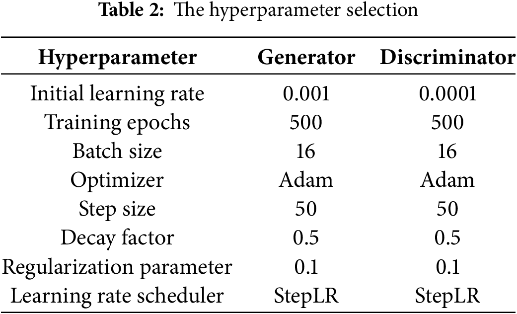
The dataset comprises 500 random field images of tensile strength and their corresponding crack propagation images and stress-strain curves from FEM simulations. It is important to note that generating this dataset is a computationally intensive process, highlighting the very bottleneck this surrogate model aims to address. This data is partitioned into 400 training and 100 testing samples. For preprocessing, crack images are converted to grayscale. Subsequently, weighted masks are generated for the loss function, where crack pixels are assigned a weight of 50. This specific weight is determined through comparative experiments, yielding optimal model performance. For training, an iterative process is adopted. Each epoch involves feeding batches of input images (random field samples) and corresponding target images (crack patterns or stress-strain curves) to the CGAN. To enhance robustness and mitigate overfitting, random flipping is employed as a data augmentation technique, alongside L2 regularization. Addressing the inherent challenges of GAN training, such as potential instability and mode collapse, required a carefully designed optimization strategy. The generator and discriminator are trained using an alternating optimization strategy. Adam optimizer is applied to both networks. The discriminator is updated first, aiming to better distinguish real from generated images while the generator remains fixed. Then, the generator is updated to create more realistic images while the discriminator’s weights are held constant. A StepLR scheduler progressively reduces the learning rate for both during training, ensuring smoother convergence. Notably, the generator’s learning rate (0.001) is set higher than the discriminator’s (0.0001). This choice helps maintain a stable adversarial balance, allowing the generator to learn more effectively without the discriminator becoming overly dominant prematurely. This strategy ensures synchronized network improvement, leading to stable training and excellent performance. Table 2 summarizes the hyperparameters and other experimental factors.

4.3.2 Model Loss Function Selection

In this study, the generator and discriminator utilize distinct loss functions, specifically optimized for crack prediction. The generator’s objective is guided by a weighted composite loss function. This loss combines three terms: perceptual loss, ensuring high-level feature similarity; L1 loss, for pixel-level accuracy; and adversarial loss, promoting realistic image generation. The weights for these terms are dynamically adjusted during training. perceptual loss receives a higher weight to quickly capture high-level features. As training progresses, the L1 loss weight increases for better alignment with image details and edges, while the adversarial loss weight remains balanced to prevent overfitting and preserve image quality. The composite loss is defined as [31,42,43]:

Ltotal=λpercLperc+λL1LL1+λadvLadv(17)

Lperc=EX,z[1C⋅H⋅W‖ϕ(G(z))−ϕ(X)‖22](18)

LL1=EX,z[∑i=1H∑j=1WWi,j⋅|G(z)i,j−Xi,j|](19)

Ladv=−Ez[log⁡D(G(z))](20)

where Lperc, LL1 and Ladv represent perceptual loss, L1 loss, and adversarial loss, respectively; C,H,W represent the number of channels, height, and width of the feature map, respectively; λperc, λL1 and λadv are the weights for each loss term ; X denotes the real image ; ϕ(X) indicates the features extracted by a pre-trained convolutional neural network; The weight W is a pre-generated mask image used to emphasize crack regions during the loss calculation.

The discriminator’s objective uses binary cross-entropy loss. It aims to classify inputs as either real or generated. The discriminator outputs a probability between 0 and 1; ideally, it should assign a probability close to 1 for real images and near 0 for generated ones. The loss function is defined as [44]:

LD=−EX[log⁡D(X)]−Ez[log⁡(1−D(G(z)))](21)

These two loss functions establish an adversarial relationship. The generator’s composite loss, particularly its adversarial component, drives it to produce outputs that the discriminator classifies as real. Concurrently, the discriminator’s binary cross-entropy loss encourages it to accurately distinguish between real and synthetic data.

The stability of the training process and model convergence are further supported by the loss curves of the generator and discriminator over 500 epochs, as illustrated in Fig. 12. The generator’s loss shows a consistent downward trend, indicating it is effectively learning to produce more realistic outputs. Simultaneously, the discriminator’s loss oscillates within a stable range, which signifies a healthy adversarial competition and prevents mode collapse. This dynamic equilibrium demonstrates that the training process converges stably.

Figure 12: Loss curves of the generator and discriminator during the training process

4.4 CGAN Model Training and Prediction Results for Stress-Strain Curve

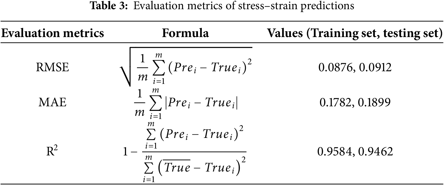
The model is trained with the Adam optimizer (learning rates: 0.001 for the generator and 0.0001 for the discriminator) over 300 epochs with a batch size of 4 and a weight decay factor of 0.001. The loss function integrates adversarial loss and L1 loss to balance curve realism and numerical accuracy. As shown in Table 3, the evaluation results indicate low Root Mean Square Error (RMSE) and Mean Absolute Error (MAE) values along with R² values close to 1 on both training and testing datasets. These results demonstrate the model’s high accuracy, stability, and strong generalization capabilities.

To further validate the model's predictive performance, Figs. 13 and 14 compare the stress-strain curves predicted by the CGAN model with those obtained from FEM simulations for two random field samples. As depicted in Figs. 13 and 14, the CGAN model effectively captures the key characteristics of stress-strain behavior, offering a computationally efficient alternative to traditional FEM simulations.

Figure 13: Stress-strain curve prediction result of Sample 1. (a) Random fields input; (b) FEM and CGAN prediction result

Figure 14: Stress-strain curve prediction result of Sample 2. (a) Random fields input; (b) FEM and CGAN prediction result

4.5 Crack Path Prediction Results

To accurately evaluate the predictive performance of the deep learning model, this study utilizes three metrics: Intersection over Union (IoU), Structural Similarity Index Measure (SSIM), and Peak Signal to Noise Ratio (PSNR). The formulas for these evaluation metrics are as follows [45,46]:

IoU=|P∩T||P∪T|(22)

SSIM=(2μPμT+C1)(2σPT+C2)(μP2+μT2+C1)(σP2+σT2+C2)(23)

PSNR=10⋅log10⁡(M2⋅N∑i=1N(Pi−Ti)2)(24)

where P and T are the binarized predicted crack image and the real crack image, respectively, with each pixel value being 0 or 1 (1 represents the crack region, 0 represents the non-crack region); |P∩T| represents the number of pixels in the intersection of the predicted and real crack images; |P∪T| represents the number of pixels in the union of the predicted and real crack images; μP and μT are the mean pixel values of the predicted and real images, respectively; σP and σT are the pixel variances of the predicted and real images, respectively; σPT is the covariance between the predicted and real images; C1 and C2 are small constants used to prevent division by zero; M is the maximum pixel value of the image; N is the total number of pixels in the image; Pi and Ti are the pixel values at the i-th position in the predicted and real images, respectively.

IoU measures overlap between predicted and actual crack areas, with higher values indicating better accuracy. SSIM evaluates image similarity in terms of luminance, contrast, and structure, where values near 1 mean greater resemblance. PSNR assesses pixel-level differences, with higher values showing better image quality and fewer errors.

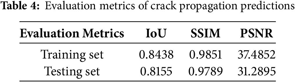
Table 4 highlights the effectiveness of the deep learning model. On the training dataset, the model achieves an IoU of 0.8438, indicating accurate localization of crack regions. A SSIM of 0.9851 further confirms the high structural fidelity between the predicted and reference images. In addition, the PSNR reaches 37.4852, suggesting that the predicted images maintain excellent visual quality with minimal pixel-wise deviation. On the testing set, the model achieves an IoU of 0.8155, an SSIM of 0.9789, and a PSNR of 31.2895.

To better illustrate the predictive performance of the CGAN model, visual comparisons are provided. Figs. 15 and 16 show the predicted crack images generated by the trained deep learning model. These results are compared with the corresponding crack patterns obtained from finite element simulations.

Figure 15: Crack propagation prediction result of Sample 1. (a) Random fields input; (b) FEM simulations result; (c) CGAN prediction result

Figure 16: Crack propagation prediction result of Sample 2. (a) Random fields input; (b) FEM simulations result; (c) CGAN prediction result

We conduct a statistical analysis of the maximum crack width from both FEM simulations and CGAN-predicted crack images on the dataset, as shown in Table 5.

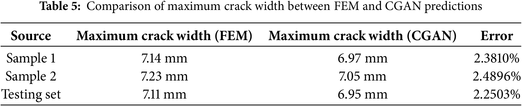
Visual and statistical analyses indicate that the CGAN model accurately predicts crack patterns, which shows good agreement with FEM results. The generated cracks reproduce both the overall shape and propagation paths. In particular, the predicted maximum crack widths align well with FEM simulation data. These results confirm the model’s generalization ability and its potential for practical use in crack prediction of quasi-brittle materials.

The predictive performance of this CGAN framework is demonstrably strong compared to other deep learning approaches for fracture prediction, such as models for porous media fracture [24] or road crack forecasting [23]. However, this framework offers a more comprehensive perspective. Unlike many existing deep learning methods focused on single prediction tasks, it achieves a holistic prediction of both stochastic crack patterns and associated stress-strain responses. Furthermore, the CGAN framework serves as an efficient surrogate model. It supports large-scale MC Simulations for comprehensive statistical evaluation of fracture behavior, a capability often computationally prohibitive for traditional FEM or many existing deep learning models.

4.6 Statistical Analysis of Crack Patterns Predicted by CGAN

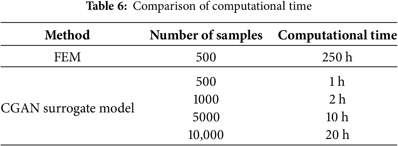
Understanding the statistical characteristics of crack patterns is essential for evaluating the structural performance and failure mechanisms in random media. However, traditional FEM simulations are computationally intensive and time-consuming, which limits their ability to perform large-scale stochastic analyses. Such analyses, like MC simulations, require many runs with random inputs to statistically evaluate system behavior. In this study, CGAN serves as a surrogate model to conduct analyses on datasets containing 1000, 5000, and 10,000 samples. It focuses on crack density and spatial distribution. Crack density reflects the extent of material damage within different regions. Spatial distribution provides insights into crack propagation paths and concentration areas. The CGAN surrogate model significantly reduces computational time compared to FEM simulations, as shown in Table 6. All FEM simulations in this study were performed using Abaqus software. Both the FEM simulations and CGAN predictions are conducted on a laptop equipped with a four-core i7 CPU and 8GB of memory. Compared to traditional FEM simulations, the CGAN surrogate model reduces computational time from 250 to 1 h for 500 samples while maintaining high predictive accuracy.

The crack initiation positions are concentrated on both sides of the specimen. To analyze crack distribution quantitatively, image processing techniques are used. These techniques extract crack pixel points on both sides of the specimen and determine crack positions. Based on this positional information, Probability Density Function (PDF) maps are generated, as shown in Fig. 17. Furthermore, all crack pixel points are extracted and aggregated to create a crack density heatmap, as illustrated in Fig. 18. In this heatmap, the color scale represents the ratio of crack occurrences at a specific location to the total number of samples. This provides further visualization of the spatial distribution characteristics of the cracks.

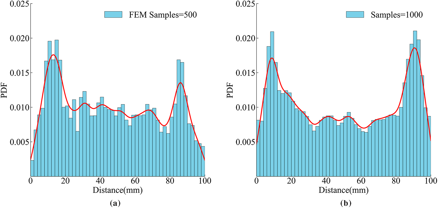
Figure 17: PDF maps of fracture location along specimen length. (a) FEM simulations samples = 500; (b) CGAN prediction Samples = 1000; (c) CGAN prediction Samples = 5000; (d) CGAN prediction Samples = 10,000

Figure 18: Crack density heatmaps of fracture location. (a) FEM simulations samples = 500; (b) CGAN prediction Samples = 1000; (c) CGAN prediction Samples = 5000; (d) CGAN prediction Samples = 10,000

Based on Figs. 17 and 18, the following conclusions can be drawn:

(1)   The PDF maps and crack density heatmaps generated by the CGAN model closely match those obtained from FEM simulations. It is demonstrated that the surrogate model can accurately reproduce the statistical distribution of crack positions. This consistency validates the reliability of the CGAN model for representing the spatial characteristics of fracture behavior.

(2)   The statistical results from both FEM and CGAN show that cracks tend to form symmetrically on both sides of the specimen, with density peaks near the boundaries. This pattern is consistent with the experimental observations [38,47] which reflects typical stress concentration under uniaxial tension. The observed agreement reinforces the credibility of the model in capturing the underlying fracture behavior.

(3)   As the sample size increases from 1000 to 10,000, the PDF curves become smoother, and the heatmaps exhibit clearer contours and more defined density regions. This demonstrates that large-sample analyses using CGAN enhance statistical convergence, enabling more robust evaluations of stochastic crack behavior.

5  Conclusions

This work presents a deep learning-based framework for predicting stochastic crack behavior in random media. By integrating CGAN with random field modeling, the proposed approach captures the spatial variability of material properties while efficiently simulating crack propagation. In contrast to conventional FEM-based methods, this model greatly reduces computational demands without compromising accuracy. The trained CGAN model serves as the surrogate model for MC Simulations to reveal statistical features, such as crack density patterns and preferential fracture zones.

The main findings of this study are as follows:

(1)   The CGAN model accurately predicts crack initiation and propagation in concrete under uniaxial tensile loading, which serves as a case study of random media. With an IoU of 0.8438 and 0.8155 on the training and testing datasets, the predicted crack patterns align well with FEM simulation results in both shape and detail. The model also achieves R² values of 0.9584 and 0.9462 for stress-strain curve prediction, which captures the overall mechanical response.

(2)   Compared to FEM, the CGAN model drastically improves computational efficiency. For 500 samples, CGAN completes predictions in 1 h, whereas FEM takes over 250 h. In the case of 10,000 samples, FEM becomes impractical, while CGAN completes the task in under 20 h. Approximately, the CGAN model achieves a computational efficiency 250 times higher than that of the FEM model in the proposed case study. This efficiency makes CGAN well-suited for large-scale stochastic fracture analysis.

(3)   The CGAN model is applied as the surrogate model, which reproduces the statistical patterns observed in FEM results. These include symmetric crack distributions and density peaks near the specimen boundaries. This agreement confirms its reliability in capturing spatial fracture characteristics. As the number of samples increases, the predicted distributions show greater smoothness. The results support the model’s effectiveness in large-scale stochastic crack evaluation.

(4)   It is important to acknowledge the limitations of the current model, which are defined by the scope of this study. The model is trained and validated solely under uniaxial tensile loading, with a focus on quasi-brittle fracture processes. However, these limitations also highlight promising avenues for future work, driven by the framework’s significant advantages in computational efficiency and its inherent extensibility. Future research should explore the model’s generalization ability under various other loading conditions, such as shear and compression. Another key direction is extending the framework to predict ductile fracture processes, broadening its applicability to a wider range of engineering materials. Achieving these expansions would require generating diverse FEM datasets and potentially modifying the CGAN’s input to explicitly include these external conditions as additional features.

Acknowledgement: None.

Funding Statement: This research was supported by the Science Foundation of Zhejiang Province of China (Grant No. LY22E080016), the National Natural Science Foundation of China (Grant No. 51808499), and the Fundamental Research Funds of Zhejiang Sci-Tech University (Grant No. 24052126-Y).

Author Contributions: The authors confirm contribution to the paper as follows: study conception and design: Shixue Liang; data collection: Junning Wu; analysis and interpretation of results, draft manuscript preparation: Xing Lin. All authors reviewed the results and approved the final version of the manuscript.

Availability of Data and Materials: Some or all data, models, or code that support the findings of this study are available from the corresponding author upon reasonable request.

Ethics Approval: Not applicable.

Conflicts of Interest: The authors declare no conflicts of interest to report regarding the present study.

Nomenclature

References

1. Zhou F, Molinari J-F. Stochastic fracture of ceramics under dynamic tensile loading. Int J Solids Struct. 2004;41:6573–96. doi:10.1016/j.ijsolstr.2004.05.029. [Google Scholar] [CrossRef]

2. Xu XF, Graham-Brady L. A stochastic computational method for evaluation of global and local behavior of random elastic media. Comput Methods Appl Mech Eng. 2005;194:4362–85. doi:10.1016/j.cma.2004.12.001. [Google Scholar] [CrossRef]

3. Koutsourelakis PS, Deodatis G. Simulation of multidimensional binary random fields with application to modeling of two-phase random media. J Eng Mech. 2006;132:619–31. doi:10.1061/(ASCE)0733-9399(2006)132:. [Google Scholar] [CrossRef]

4. Ren X, Li J. Dynamic fracture in irregularly structured systems. Phys Rev E. 2012;85(5):055102. doi:10.1103/PhysRevE.85.055102. [Google Scholar] [PubMed] [CrossRef]

5. Liang S, Ren X, Li J. A random medium model for simulation of concrete failure. Sci China Technol Sci. 2013;56(5):1273–81. doi:10.1007/s11431-013-5200-y. [Google Scholar] [CrossRef]

6. Park K, Paulino GH. Cohesive zone models: a critical review of traction-separation relationships across fracture surfaces. Appl Mech Rev. 2013;64(6):060802. doi:10.1115/1.4023110. [Google Scholar] [CrossRef]

7. Wu J-Y, Yao J-R, Le J-L. Phase-field modeling of stochastic fracture in heterogeneous quasi-brittle solids. Comput Methods Appl Mech Eng. 2023;416(17):116332. doi:10.1016/j.cma.2023.116332. [Google Scholar] [CrossRef]

8. Zhang H, Huang Y, Hu X, Xu S. A quasi-brittle fracture investigation of concrete structures integrating random fields with the CSFEM-PFCZM. Eng Fract Mech. 2023;281(9):109107. doi:10.1016/j.engfracmech.2023.109107. [Google Scholar] [CrossRef]

9. Wu J, Liu W, Liang S. Multiscale random damage analysis through deep learning-driven surrogate models. Int J Multiscale Comput Eng. 2025;23(4):27–48. doi:10.1615/IntJMultCompEng.2024054201. [Google Scholar] [CrossRef]

10. Wang F, Zhai W, Man J, Huang H. A hybrid cohesive phase-field numerical method for the stability analysis of rock slopes with discontinuities. Can Geotech J. 2025;62(7):1–16. doi:10.1139/cgj-2024-0382. [Google Scholar] [CrossRef]

11. Petrie C, Oudah F. Stochastic finite element approach to assess reliability of fiber-reinforced polymer-strengthened concrete beams. ACI Struct J. 2023;120(6):193–208. doi:10.14359/51739096. [Google Scholar] [CrossRef]

12. Herrod J. Random field modeling of microstructure in unidirectional fiber-reinforced plastic using sem-image and image processing for multiscale stochastic stress analysis considering random fiber arrangements. Adv Eng Mater. 2022;24(5):2270020. doi:10.1002/adem.202270020. [Google Scholar] [CrossRef]

13. Zhang H, Huang Y, Yang Z, Guo F, Shen L. 3D meso-scale investigation of ultra high performance fibre reinforced concrete (UHPFRC) using cohesive crack model and Weibull random field. Constr Build Mater. 2022;327(48):127013. doi:10.1016/j.conbuildmat.2022.127013. [Google Scholar] [CrossRef]

14. Ghannoum M, Baroth J, Millard A, Rospars C. Stochastic finite element modeling of heterogeneities in massive concrete and reinforced concrete structures. Int J Numer Anal Methods Geomech. 2024;48(5):1227–44. doi:10.1002/nag.3684. [Google Scholar] [CrossRef]

15. Kala Z, Valeš J, Jönsson J. Random fields of initial out of straightness leading to column buckling. J Civ Eng Manage. 2017;23(7):902–13. doi:10.3846/13923730.2017.1341957. [Google Scholar] [CrossRef]

16. Wang X, Yang Z, Jivkov AP. Monte carlo simulations of mesoscale fracture of concrete with random aggregates and pores: a size effect study. Constr Build Mater. 2015;80:262–72. doi:10.1016/j.conbuildmat.2015.02.002. [Google Scholar] [CrossRef]

17. Wang X, Li P, Jia K, Zhang S, Li C, Wu B, et al. SPI-MIONet for surrogate modeling in phase-field hydraulic fracturing. Comput Methods Appl Mech Eng. 2024;427(6):117054. doi:10.1016/j.cma.2024.117054. [Google Scholar] [CrossRef]

18. Tong T, Li X, Wu S, Wang H, Wu D. Surrogate modeling for the long-term behavior of PC bridges via FEM analyses and long short-term neural networks. Structures. 2024;63(7):106309. doi:10.1016/j.istruc.2024.106309. [Google Scholar] [CrossRef]

19. Barkhordari MS, Armaghani DJ, Asteris PG. Structural damage identification using ensemble deep convolutional neural network models. Comput Model Eng Sci. 2022;134(2):835–55. doi:10.32604/cmes.2022.020840. [Google Scholar] [CrossRef]

20. Yang Y, Zhang G, Xu W, Zhu Y, Su L. A novel detection method for pavement crack with encoder-decoder architecture. Comp Model Eng Sci. 2023;137(1):761–73. doi:10.32604/cmes.2023.027010. [Google Scholar] [CrossRef]

21. Mayya AM, Alkayem NF. Enhance the concrete crack classification based on a novel multi-stage YOLOV10-ViT framework. Sens. 2024;24(24):8095. doi:10.3390/s24248095. [Google Scholar] [PubMed] [CrossRef]

22. Amieghemen GE, Ramezani M, Sherif MM. Residual pyramidal GAN (RP-GAN) for crack detection and prediction of crack growth in engineered cementitious composites. Measurement. 2025;242(8):115769. doi:10.1016/j.measurement.2024.115769. [Google Scholar] [CrossRef]

23. Sekar A, Perumal V. CFC-GAN: forecasting road surface crack using forecasted crack generative adversarial network. IEEE Trans Intell Transp Syst. 2022;23(11):21378–91. doi:10.1109/TITS.2022.3171433. [Google Scholar] [CrossRef]

24. He Y, Tan Y, Yang M, Wang Y, Xu Y, Yuan J, et al. Accurate prediction of discontinuous crack paths in random porous media via a generative deep learning model. Proc Natl Acad Sci. 2024;121(40):e2413462121. doi:10.1073/pnas.2413462121. [Google Scholar] [PubMed] [CrossRef]

25. Zhao S, Wang F-Y, Tan D-Y, Yang A-W. A deep learning informed-mesoscale cohesive numerical model for investigating the mechanical behavior of shield tunnels with crack damage. Structures. 2024;66(5):106902. doi:10.1016/j.istruc.2024.106902. [Google Scholar] [CrossRef]

26. Xu H, Fan W, Ruan L, Shi R, Taylor AC, Zhang D. Crack-net: a deep learning approach to predict crack propagation and stress–strain curves in particulate composites. Engineering. 2025;49(14):149–63. doi:10.1016/j.eng.2025.02.022. [Google Scholar] [CrossRef]

27. Shinozuka M, Deodatis G. Simulation of multi-dimensional gaussian stochastic fields by spectral representation. Appl Mech Rev. 1996;49(1):29–53. doi:10.1115/1.3101883. [Google Scholar] [CrossRef]

28. Dannert MM, Faes MGR, Fleury RMN, Fau A, Nackenhorst U, Moens D. Imprecise random field analysis for non-linear concrete damage analysis. Mech Syst Signal Process. 2021;150(1):107343. doi:10.1016/j.ymssp.2020.107343. [Google Scholar] [CrossRef]

29. Barenblatt GI. The mathematical theory of equilibrium cracks in brittle fracture. In: Dryden HL, von Kármán Th, Kuerti G, van den Dungen FH, Howarth L, editors. Advances in applied mechanics. Vol. 7. Amsterdam, The Netherlands: Elsevier; 1962. p. 55–129. doi:10.1016/S0065-2156(08)70121-2. [Google Scholar] [CrossRef]

30. Goodfellow I, Pouget-Abadie J, Mirza M, Xu B, Warde-Farley D, Ozair S, et al. Generative adversarial networks. Commun ACM. 2020;63(11):139–44. doi:10.1145/3422622. [Google Scholar] [CrossRef]

31. Mirza M, Osindero S. Conditional generative adversarial nets. arXiv:1411.1784. 2014. doi:10.48550/arXiv.1411.1784. [Google Scholar] [CrossRef]

32. He K, Zhang X, Ren S, Sun J. Deep residual learning for image recognition. In: 2016 IEEE Conference on Computer Vision and Pattern Recognition (CVPR); 2016 Jun 27–30; Las Vegas, NV, USA. p. 770–8. doi:10.1109/CVPR.2016.90. [Google Scholar] [CrossRef]

33. Li C, Wand M. Precomputed real-time texture synthesis with markovian generative adversarial networks. In: Leibe B, Matas J, Sebe N, Welling M, editors. Computer Vision—ECCV 2016. Cham, Switzerland: Springer International Publishing; 2016. p. 702–16. doi:10.1007/978-3-319-46487-9_43. [Google Scholar] [CrossRef]

34. Xu B, Wang N, Chen T, Li M. Empirical evaluation of rectified activations in convolutional network. arXiv.1505.00853. 2015. doi:10.48550/arXiv.1505.00853. [Google Scholar] [CrossRef]

35. Maas AL, Hannun AY, Ng AY. Rectifier nonlinearities improve neural network acoustic models. Proc ICML. 2013;30:3 [Google Scholar]

36. Guan J, Li C, Wang J, Qing L, Song Z, Liu Z. Determination of fracture parameter and prediction of structural fracture using various concrete specimen types. Theor Appl Fract Mech. 2019;100:114–27. doi:10.1016/j.tafmec.2019.01.008. [Google Scholar] [CrossRef]

37. Bažant ZP, Pijaudier-Cabot G. Measurement of characteristic length of nonlocal continuum. J Eng Mech. 1989;115:755–67. doi:10.1061/(ASCE)0733-9399(1989)115. [Google Scholar] [CrossRef]

38. Ren X, Yang W, Zhou Y, Li J. Behavior of high-performance concrete under uniaxial and biaxial loading. ACI Mater J. 2008;105(6):548–58. doi:10.14359/20196. [Google Scholar] [CrossRef]

39. Carpinteri A, Chiaia B. Size effects on concrete fracture energy: dimensional transition from order to disorder. Mater Struct. 1996;29(5):259–66. doi:10.1007/BF02486360. [Google Scholar] [CrossRef]

40. Carpinteri A, Chiaia B, Ferro G. Size effects on nominal tensile strength of concrete structures: multifractality of material ligaments and dimensional transition from order to disorder. Mater Struct. 1995;28(6):311–7. doi:10.1007/BF02473145. [Google Scholar] [CrossRef]

41. Bruggi M, Casciati S, Faravelli L. Cohesive crack propagation in a random elastic medium. Probab Eng Mech. 2008;23(1):23–35. doi:10.1016/j.probengmech.2007.10.001. [Google Scholar] [CrossRef]

42. Isola P, Zhu J-Y, Zhou T, Efros AA. Image-to-image translation with conditional adversarial networks. In: Proceedings of the IEEE Conference on Computer Vision and Pattern Recognition; 2017 Jul 21–26; Honolulu, HI, USA. p. 1125–34. doi:10.48550/arXiv.1611.07004. [Google Scholar] [CrossRef]

43. Johnson J, Alahi A, Fei-Fei L. Perceptual losses for real-time style transfer and super-resolution. In: Leibe B, Matas J, Sebe N, Welling M, editors. Computer vision—ECCV 2016. Cham, Switzerland: Springer International Publishing; 2016. p. 694–711. [Google Scholar]

44. Cox DR. The regression analysis of binary sequences. J R Stat Soc B. 2018;20(2):215–32. doi:10.1111/j.2517-6161.1958.tb00292.x. [Google Scholar] [CrossRef]

45. Wang Z, Bovik AC, Sheikh HR, Simoncelli EP. Image quality assessment: from error visibility to structural similarity. IEEE Trans Image Process. 2004;13(4):600–12. doi:10.1109/TIP.2003.819861. [Google Scholar] [PubMed] [CrossRef]

46. Yu J, Jiang Y, Wang Z, Cao Z, Huang T. UnitBox: an advanced object detection network. In: Proceedings of the 24th ACM International Conference on Multimedia;2016 Oct 15–19; Amsterdam, The Netherlands. p. 516–20. doi:10.1145/2964284.2967274. [Google Scholar] [CrossRef]

47. Xu G, Jia N, Li Y, Li C, Peng Y. New method for uniaxial tensile test of UHPFRC. Eng Fract Mech. 2025;316(6):110900. doi:10.1016/j.engfracmech.2025.110900. [Google Scholar] [CrossRef]