Numerical Modeling of Bubble-Particle Attachment in a Volume-of-Fluid Framework

1  Introduction

Gas bubbles are widely used to capture particles in various industrial applications, such as recovery of coal and minerals from ores, de-inking in paper recycling, and inclusion removal in steelmaking processes [1]. In particular, inclusion removal using gas bubbles is a key technique for producing ultra-clean steel, where micro-sized inclusions are collected on bubble surfaces by injecting gas at various locations [2]. Numerical simulations of particle attachment to bubble surfaces are valuable for improving these applications. However, predicting particle attachment requires an understanding of complex three-phase flow, which makes it challenging to determine the optimal locations for gas injection and improve inclusion removal efficiency.

Particle attachment to a bubble surface is governed primarily by three phenomena: oscillating collision, liquid film formation, and sliding. When a flow-driven particle contacts a bubble, oscillations occur due to the particle inertia and surface tension. Meanwhile, a thin liquid film forms between the particle and the bubble surface, causing the particle to slide downward. The particle may continue sliding and eventually detach, or it may attach to the bubble when the liquid film ruptures. This attachment process can be characterized by three timescales corresponding to each phenomenon: collision time, induction time, and sliding time. The collision time corresponds to the duration of the oscillating collision, for which a mathematical expression was proposed by Evans [3]. The induction time denotes the lifetime of the liquid film from formation to rupture. Finally, the sliding time characterizes the interval during which the particle slides over the bubble surface. This phenomenon was modeled by adopting experimental results [4,5] under the assumptions of inertialess particles and potential flow [6].

Recent efforts have examined bubble-particle interactions using advanced CFD and modeling approaches. Liu et al. [7] and Li et al. [8] reported particle-scale insights into fluidization and phase distribution, while Wang et al. [9] reviewed CFD applications in flotation. Chan et al. [10] investigated bubble-particle collisions under turbulence, and Zheng et al. [11] proposed a model for predicting collision efficiency. In parallel, Szmigiel et al. [12] highlighted the role of machine learning in flotation process optimization. These studies underscore recent progress, though attachment and detachment dynamics remain insufficiently addressed. Many researchers have studied bubble–particle attachment phenomena using numerical methods. To predict collision efficiency and attachment probability, hydrophobic forces acting on particles near a stationary bubble have been modeled [13–15]. It was concluded in the previous work that the force acting on particles near a bubble has a significant impact on predicting bubble–particle interactions. Although these studies have simulated particle motions near bubble surfaces based on attachment physics, only the particle dynamics are solved without consideration of the dynamics of the flow field. Some studies have incorporated flow field results to estimate collision efficiency [16–19]. To better capture particle behavior around deformable bubble surfaces, the volume-of-fluid (VOF) method has been employed to model the phase interface in gas-liquid-solid systems [20–22]. Further advances extended this approach to multiscale and coupled DEM-VOF methods [23,24]. More recently, particle-bubble interactions near solid boundaries have also been investigated using VOF-based simulations [25]. However, the detailed physics of particle attachment at the bubble surface has not been considered in these studies.

Despite numerous theoretical models on attachment physics, it has been difficult to apply them to practical numerical methods for multiphase flow such as those based on a VOF method. Liu et al. [26] provided a detailed assessment and analysis of five different phase-change models for simulating vapor bubble condensation within a VOF framework. Although bubble-particle interactions were not considered in this study, the method integrated physical bubble models with the VOF method. To accurately predict attachment, the three characteristic times related to bubble-particle interaction must be accounted for. Especially, calculating the induction time has been difficult because modeling the physics of the liquid film is complex. According to Nguyen et al. [27], the characteristic times can be alternatively interpreted as the relative position between a particle and a bubble. By adopting the concept of a critical angle, induction and sliding times can instead be represented by geometric relations between a particle and a bubble. In this model, the collision location of a particle to the bubble surface must be known a priori. However, when the bubble interface and the particles are represented in a distinct Eulerian–Lagrangian framework, the accuracy of the interface reconstruction is affected by grid resolution [28]. For this reason, precise determination of the collision location is technically difficult.

In the present study, bubble-particle attachment is modeled by considering both the attachment physics and the dynamics of the bubble surface. To apply the theoretical relationship developed by Nguyen et al. [27] to an Eulerian-Lagrangian framework based on a VOF method, an effective bubble is introduced to predict the collision locations. A method for computing the bubble-particle angle is devised to determine the three characteristic times: collision, induction, and sliding times, during bubble-particle interaction. Numerical algorithms are developed to incorporate both the VOF method and the relationship proposed by Nguyen et al. [27].

Numerical methods for simulating gas-liquid-solid flows are described in Section 2. The physical background and numerical algorithms for bubble-particle interaction are presented in Sections 3 and 4, respectively. Results of validation simulations using the present numerical method are discussed in Section 5, followed by concluding remarks in Section 6.

2  Numerical Methods

2.1 Governing Equations

Gas-liquid flow is governed by the Navier-Stokes equations with surface tension. The one-fluid formulation is adopted, in which the total density and total dynamic viscosity are used instead of solving the governing equations separately for each phase. The incompressible variable-density Navier-Stokes equations in Cartesian coordinates are given as follows:

∂ui∂xi=0,(1)

∂ui∂t+∂uiuj∂xj=−1ρ∂p∂xi+1ρ∂∂xj(µ(∂ui∂xj+∂uj∂xi))+gi+fσiρ,(2)

where ui, p, ρ, µ, gi, and fσi denote the velocity, pressure, total density, total dynamic viscosity, gravitational acceleration, and surface tension force, respectively. The total density and total dynamic viscosity are defined as follows:

ρ(c)=cρg+(1−c)ρl,(3)

µ(c)=cµg+(1−c)µl,(4)

where c is the volume fraction of the gas phase, and the subscripts g and l denote the gas and liquid phases, respectively.

Numerical schemes for solving Eqs. (1) and (2) are described in [29]. The Crank–Nicolson scheme is employed for time advancement, and a Newton-iterative method is applied to solve the nonlinear terms. A second-order central-difference scheme is used to discretize the spatial derivative terms. The fractional-step method and an approximate factorization technique [30] are then applied to the discretized equations. Finally, the Poisson equation for pressure is solved using an algebraic multigrid method [31].

The motion of a solid particle is predicted within a Lagrangian framework. The governing Lagrangian equations for the particle motion are expressed as follows:

dxpdt=up,(5)

dupdt=fStp(u−up),(6)

where xp, up, u, f, and Stp denote the particle position, particle velocity, fluid velocity, drag coefficient, and particle Stokes number, respectively. Crowe et al. [32] suggested that the drag coefficient can be modeled as follows:

f=(1+0.15Rep0.687),(7)

where Rep is the particle Reynolds number. The particle Stokes number Stp is defined as follows:

Stp=118ρpdp2µ,(8)

where ρp and dp denote the particle density and particle diameter, respectively. Eqs. (5) and (6) are solved using a third-order Runge–Kutta method. The fluid velocity u at the particle position xp is obtained using the fourth-order Lagrange polynomial interpolation.

2.2 Volume-of-Fluid Method

The gas and liquid phases are distinguished by the volume fraction, which is advected using the VOF method. The advection equation for the volume fraction c is written as follows:

∂c∂t+ui∂c∂xi=0.(9)

A piecewise linear interface calculation (PLIC) approach [33] is used to solve Eq. (9). In this approach, the phase interface in each cell is represented by a line or a plane equation. The VOF/PLIC method consists of two steps. First, the interface is reconstructed from the volume fraction c. The reconstruction step requires estimating the normal vector and the plane constant of the interface. The interface in each cell is represented as follows:

ni⋅xi=α,(10)

where ni, xi, and α denote the local normal vector of the interface, the position vector, and the plane constant of the interface, respectively. In the present study, the normal vector ni is calculated using the mixed Youngs-centered (MYC) method, as suggested by Aulisa et al. [34]. The plane constant α is then obtained analytically from the geometrical relation between the normal vector ni and the volume fraction c [35]. After the reconstruction step, the volume fraction c is advected by Eq. (9) using geometric flux computation. The conservative advection scheme of Weymouth and Yue [36] is adopted to ensure that the error in mass conservation is within the range of machine accuracy. Finally, the total density ρ and total dynamic viscosity µ are updated from Eqs. (3) and (4) using the new volume fraction.

The surface tension force fσi is evaluated at the phase interface. It is calculated using the continuum surface force method of Brackbill et al. [37]:

fσi=σκ∂c∂xi,(11)

where σ and κ are the surface tension coefficient and the curvature of the phase interface, respectively. The curvature κ is calculated by the height function method combined with the paraboloid-fitted method developed by Popinet [38]. The sharpness of the surface tension is conserved by implementing a balanced force algorithm proposed by Francois et al. [39].

3  Physics of Bubble-Particle Interaction

3.1 Mechanisms of Sliding and Attachment of a Colliding Particle

Numerical modeling of bubble-particle interaction requires understanding how a particle moves on a bubble surface. In this study, the case where the particle size is much smaller than the bubble size: the particle diameter dp is less than 0.1 times of the minimum bubble diameter db is considered. Under this condition, the attached particle do not detach from the bubble surface [40]. A particle remains attached when the adhesion force, consisting of van der Waals, capillary, and electrostatic contributions, exceeds the detaching force, which includes gravity, fluid drag, and mechanical effects. For very small particles, the mass (and thus the gravitational force) is negligible, while the surface area relative to mass is large. Consequently, surface-dependent adhesive forces readily overpower gravity, drag, and other mass-dependent detaching forces. A Capillary number less than 0.1 is considered, indicating that surface tension dominates over particle inertia. Consequently, the particle cannot deform the bubble surface [28]. The maximum Stokes number of a particle is on the order of 10−2, which justifies one-way coupling between the Eulerian flow field and the Lagrangian particle.

The motion of particles on the bubble surface can be characterized by three characteristic timescales, as illustrated in Fig. 1. These times determine whether a particle attaches or slides away after collision. The collision time tc refers to the duration of oscillation before sliding. The sliding time ts corresponds to the period during which the particle slides over the bubble surface. The induction time ti denotes the lifetime of the thin liquid film, from its formation to rupture. In Fig. 1c, the upper circle represents a particle, and the lower circle represents a bubble. The dashed lines indicate the thin liquid film formed between the bubble and the particle. The thickness of this film decreases progressively until rupture occurs. The thin liquid film plays a crucial role in determining whether a colliding particle slides away or attaches. While the thin liquid film exists, the particle continues to slide because it interrupts the attractive force between the particle and the bubble surface. In other words, attachment occurs only when tc or ts exceeds ti. If tc>ti, the thin liquid film ruptures during particle oscillation, resulting in attachment. If ts>ti, the thin liquid film ruptures during sliding, also leading to attachment. Conversely, if ts⩽ti, the film remains intact and the particle slides away.

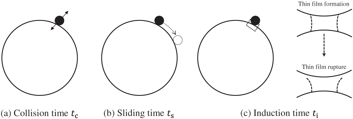
Figure 1: Schematic illustration of the three characteristic times which determine particle motions on a bubble surface: (a) collision time tc; (b) sliding time ts; and (c) induction time ti

Particle motions on the bubble surface can also be described in terms of the relative position between the bubble and the particle. The relative position is represented by the angle measured from the stagnation point (the top position of a rising spherical bubble) to the point of particle contact. Three possible outcomes after particle collision are illustrated in Fig. 2 based on the angle criteria. Three characteristic angles are used to determine particle motions. The bubble-particle angle θo is the angle at the particle position from the stagnation point. The critical angle θcr is the angle beyond which no attachment occurs. The collision angle θm is the angle beyond which no collision occurs. By the definition, no collision occurs when θo>θm. If θcr⩽θo⩽θm, the particle collides but slides away because the collision point lies beyond the critical angle θcr. If θo<θcr, the particle attaches.

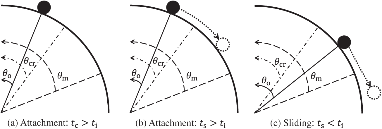
Figure 2: Schematic illustration of three types of particle motions after collision: (a) attachment during oscillation; (b) attachment during sliding; and (c) sliding over a thin liquid film

In the present model, both time and angle criteria are used to determine the particle motion. The calculation procedures for the collision angle θm and the critical angle θcr are described in the following section.

3.2 Collision and Attachment Probabilities

Based on particle motions on the bubble surface, the number of colliding and attached particles, and thereby the probabilities of collision and attachment are determined. The collision probability Pc is defined as the ratio of the actual number of colliding particles to the ideal number of colliding particles [27], as follows:

Pc=NcrNci,(12)

where Nci denotes the ideal number of colliding particles, and Ncr is the actual number of colliding particles. Fig. 3 schematically illustrates how particles collide with the bubble surface. An ideal collision implies that all particles within the bubble-sweep path collide with the bubble surface. If the position of a particle lies within the bubble radius rb, the particle ideally collides with the bubble surface. In contrast, an actual collision occurs when the particle position is within the collision radius rOC. From these definitions, the collision probability Pc can be calculated geometrically as follows:

Pc=πrOC2πrb2=(rOCrb)2=(rbsin⁡θmrb)2,(13)

where πrb2 denotes the area of ideal collision, while πrOC2 denotes the area of actual collision.

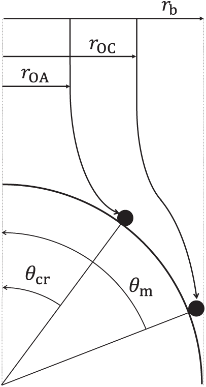
Figure 3: Definitions of the collision radius rOC and attachment radius rOA in terms of the collision angle θm and critical angle θcr

The collision probability Pc can also be modeled in terms of material properties and flow conditions [41], as follows:

Pc=2ubD9(ub+up)Y(dpdb)2[(X+C)2+3Y2+2(X+C)]2,(14)

where the dimensionless parameters X, Y, C, and D are defined as follows:

X=32+9Reb32+9.888Reb0.694,(15a)

Y=3Reb8+1.736Reb0.518,(15b)

C=upub(dbdp)2,(15c)

D=(X+C)2+3Y2−(X+C)3Y,(15d)

where ub,up, and Reb=ρlubdb/µl denote the bubble velocity, particle velocity, and bubble Reynolds number, respectively. To evaluate Eq. (14), the bubble and particle velocities must be obtained from material properties. For a rising single bubble, the bubble velocity ub can be empirically determined as follows [42]:

ub=0.138g0.82(ρlµl)0.639db1.459for  db<1.3 mm.(16)

The particle velocity can also be determined using the formula of Oeters [43], as follows:

up=(ρl−ρp)dp2g18µl,(17)

where ρp denotes the particle density. Eqs. (16) and (17) are substituted into Eq. (14) to obtain the collision probability. The collision angle θm is then evaluated using Eqs. (13) and (14).

The attachment probability Pa is defined as the ratio of the number of attached particles to the number of colliding particles [27], as follows:

Pa=NaNcr,(18)

where Na denotes the number of attached particles. Actual attachment occurs when the particle position lies within the attachment radius rOA (see Fig. 3). A value of Pa=1 indicates that all colliding particles are attached to the bubble surface. In the same manner as the collision probability, the attachment probability Pa can be defined as follows:

Pa=πrOA2πrOC2=(rOArOC)2=(rbsin⁡θcrrbsin⁡θm)2,(19)

where πrOA2 denotes the area of particle attachment.

In the present study, the attachment probability Pa is fitted to the experimental measurements of Hewitt et al. [44] An exponential form is adopted as follows:

Pa=C1×exp⁡(dp×C2),(20)

where the model constants C1 and C2 are defined as

C1=−0.4382×103×db+3.9173×sin⁡(θcont/2)−0.4581,(21a)

C2=−31.86×db−8.7973×sin⁡(θcont/2)+3.34×10−3,(21b)

where θcont denotes the contact angle. The critical angle θcr can then be calculated using the collision angle θm together with Eqs. (19) and (20).

4  Numerical Modeling of Collision, Sliding, and Attachment

In the present numerical method, particle motions including collision, sliding, and attachment, are predicted using time and angle criteria derived from empirical relationships. The numerical method consists of two steps: first, detecting particle collisions near the bubble surface; second, determining whether the colliding particle slides or attaches. Fig. 4 schematically illustrates the procedure for modeling bubble-particle interaction. The detailed algorithms and methodology are presented in the following subsections.

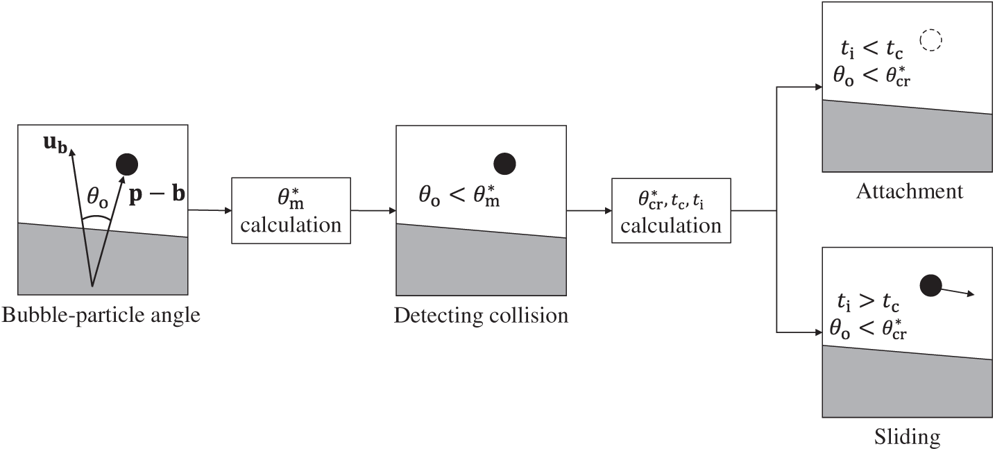
Figure 4: Procedure for modeling bubble-particle interaction. The method of calculating the bubble-particle angle θo is described in Section 4.1. The effective contact angle θm∗ and the critical angle θcr∗ are explained in Section 4.3. The algorithm for detecting collision is presented in Section 4.4. The calculation procedures for the collision time tc and induction time ti, as well as the algorithm for determining sliding or attachment, are described in Section 4.5

4.1 Relative Position and Angle between a Bubble and a Particle

As mentioned in Section 3.1, angle criteria are used to determine particle motions on the bubble surface. To apply these criteria, the bubble-particle angle θo is required. This angle is calculated from the position relationship between the bubble surface and a particle within a single cell (see Fig. 5).

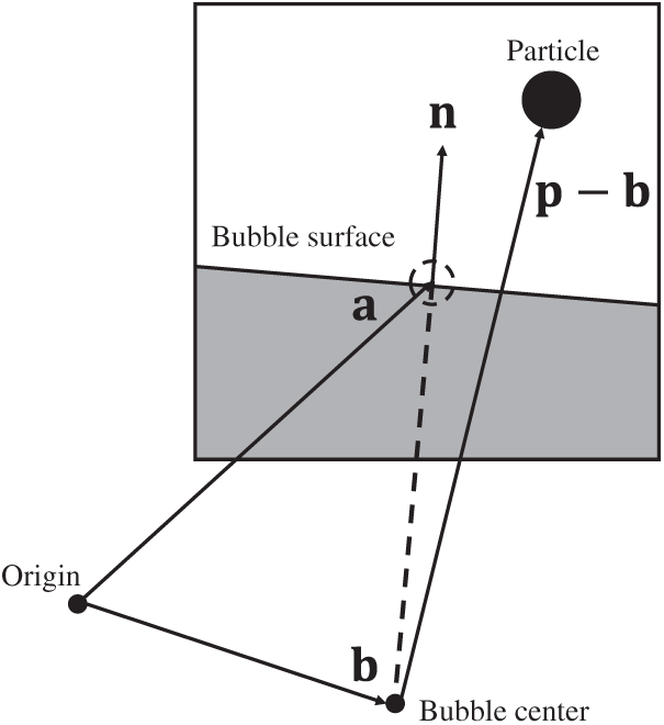
Figure 5: Position relationships between a bubble and a particle. a is the vector from the coordinate origin to the bubble surface center. n is the normal vector of the bubble surface. b is the vector from the coordinate origin to the bubble center. p is the vector from the coordinate origin to the particle center. p−b is the vector from the bubble center to the particle center

First, the normal vector of the bubble surface n is calculated using the geometric VOF method described in Section 2.2. p is the vector from the coordinate origin to the particle center. a is the vector from the coordinate origin to the center of the bubble surface, which corresponds to the center of the plane equation representing the bubble surface. This location is obtained by calculating the center of the plane equation. Finally, b is the vector from the coordinate origin to the bubble center. Fig. 5 shows that the direction of the bubble-surface normal vector n corresponds to a−b. The distance between the bubble surface and the bubble center is the bubble radius rb, calculated from the bubble curvature obtained by the VOF method as rb=2/κ. Using this relation, the position vector of the bubble center b can be calculated as follows:

b=a−βn,(22)

where β=rb/|n|.

Finally, the particle position vector relative to the bubble center p−b can be obtained. The bubble-particle angle θo is defined as the angle between the bubble velocity ub and the relative particle position vector p−b. Based on this definition, θo is calculated using the inner product formula as follows:

θo=arccos⁡(ub⋅(p−b)|ub||p−b|).(23)

4.2 Effective Bubble

Determination of particle attachment on the bubble surface begins with detecting bubble-particle collisions, since attachment is examined only for colliding particles. A collision occurs when the particle is in physical contact with the bubble surface. In other words, the collision condition is satisfied when the bubble-particle distance equals the particle radius. The bubble-particle distance db-p is defined as the distance between the particle center and the bubble surface. For the Ni-th particle, db-p can be calculated as follows:

db-p=|n⋅pNi−α||n|,(24)

where pNi denotes the position vector of the Ni-th particle.

However, a new definition of collision is required because the exact collision location cannot be easily determined: the bubble surface represented in a computational domain is not explicitly defined in the VOF method. Instead, the interface is reconstructed from the volume fraction in an Eulerian framework. Since the particle size is smaller than the grid size, calculating the exact distance between the particle center and the bubble surface is not straightforward.

In the present method, the concept of an effective bubble is introduced to address the difficulty of determining the collision location. The effective bubble is defined as having a larger diameter than the actual bubble but the same center. Fig. 6 illustrates the regions of the actual and effective bubbles. The circle with a solid line represents the actual bubble with the diameter db, while the circle with a dashed line represents the effective bubble with diameter db+2×d∗. The size of the effective bubble is controlled by d∗, which can be adjusted according to the grid resolution used in the VOF simulation. It is recommended that d∗ be larger than the largest particle diameter. In the present work, d∗ is set to 10% larger than the largest particle diameter.

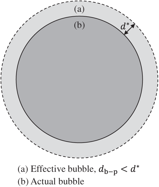
Figure 6: Definitions of (a) the effective bubble and (b) the actual bubble. db−p denotes the distance from the bubble surface to the particle center. The actual bubble has diameter db, while the effective bubble has diameter db+2×d∗

Instead of predicting the exact collision on the actual bubble surface, which is difficult to determine precisely, a collision is assumed to occur when a particle is located within the region between the effective and actual bubble surfaces. Thus a particle positioned between the solid and dashed lines in Fig. 6 is considered a candidate for collision with the actual bubble. For such colliding particles, the bubble-particle angle θo is then calculated to determine whether the particle collides and attaches to the actual bubble, using the time and angle criteria introduced in Section 3.1.

4.3 Effective Collision and Critical Angles

As mentioned in the previous section, collision and attachment are determined when a particle crosses the surface of the effective bubble. Since the collision point shifts from the actual bubble to the effective bubble, the collision and critical angles must be adjusted. Fig. 7 shows the geometric definitions of the effective collision angle θm∗ and the effective critical angle θcr∗. In the present work, effectiveness factors km and kcr are applied to the original collision angle θm and critical angle θcr. The effective collision angle θm∗ and effective critical angle θcr∗ are defined as follows:

θm∗=km×θm,(25a)

θcr∗=kcr×θcr.(25b)

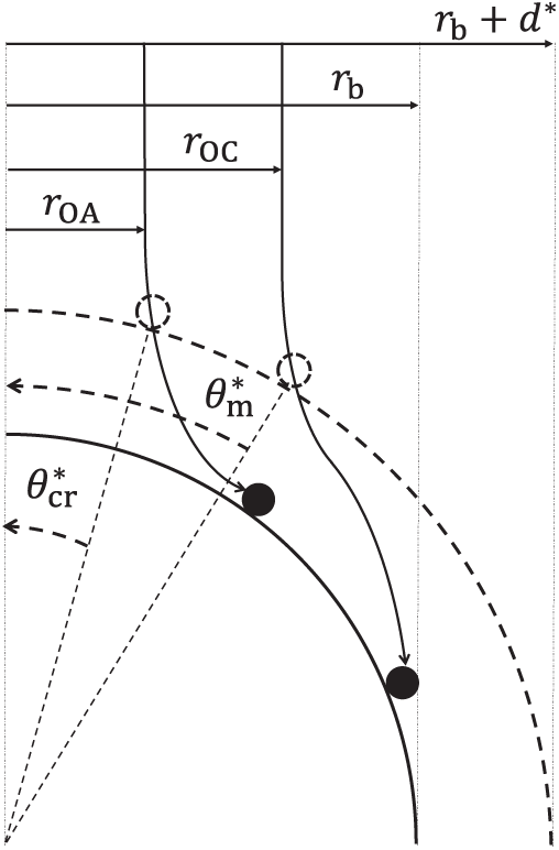
Figure 7: Effective collision angle θm∗ and effective critical angle θcr∗ with the collision radius rOC and attachment radius rOA. The solid line represents the actual bubble surface, while the dashed line represents the effective bubble surface

Details of the effectiveness factors km and kcr, as well as the tuning process, are provided in Appendix A.

4.4 Collision Detection

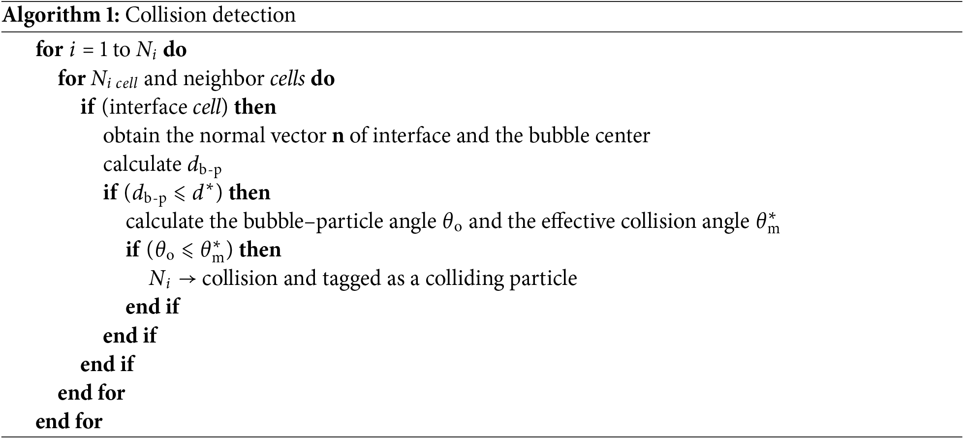
The algorithm for collision detection in the VOF method is summarized in Algorithm 1. An interface cell is defined as a cell with volume fraction c between 0 and 1. First, the existence of an interface is examined for each particle after updating its position. For example, if the cell index containing the particle is (i,j,k), then neighbor cells with indices (i±1,j±1,k±1) are examined. If an interface cell is found, the interface normal vector n and the position of the bubble center are obtained using the geometrical VOF method. The bubble–particle distance db-p is then calculated using Eq. (24). If db-p⩽d∗, the particle is considered within the effective bubble. In this case, the bubble–particle angle θo and effective collision angle θm∗ are calculated. A collision is finally confirmed by comparing the two angles: if θo⩽θm∗, the particle is tagged as a colliding particle.

4.5 Determination of Sliding or Attachment

After detecting a collision, the final step is to determine whether the colliding particle slides off or attaches to the bubble surface using the time and angle criteria. First, the collision time tc and induction time ti are computed. The collision time tc is modeled using the formulation of Evans [3], which is nearly identical to the mean value of other collision-time relationships [2]. The collision time tc is expressed as follows:

tc=(π2ρp12σ)12dp32.(26)

This timescale represents the duration of oscillation following particle collision. The induction time ti modeled by Nguyen et al. [27] is expressed as follows:

ti=dp+db2ub(1−B2)Aln⁡{tan⁡(θm2)tan⁡(θcr2)[csc⁡θm+Bcot⁡θmcsc⁡θcr+Bcot⁡θcr]B},(27)

where the dimensionless parameters A and B are given by

A=upub+dpdbX−(dpdb)2[94+2764Reb−0.2266Reb1.1274],(28a)

B=dpdbYA−0.437A(dpdb)2Reb1.0562,(28b)

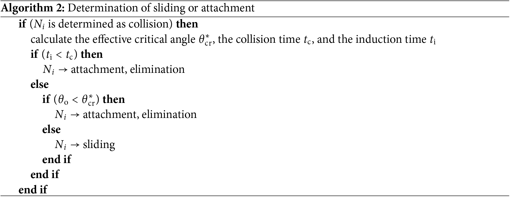
where X and Y are defined by Eqs. (15a) and (15b), respectively. The effective critical angle θcr∗ is obtained from Eq. (25b).

The procedure for determining sliding or attachment is summarized in Algorithm 2. As discussed in Section 3.1, if ti<tc, the colliding particle attaches to the bubble surface because the thin liquid film ruptures during oscillation. Otherwise, the bubble–particle angle θo and the effective critical angle θcr∗ are compared. If θo<θcr∗, the particle is considered attached to the bubble surface and is removed from the Lagrangian computation.

5  Results and Discussion

5.1 A Rising Bubble through a Layer of Particles

Numerical simulations of a rising bubble moving through a layer of many particles, as configured in Fig. 8, are conducted to present gas–liquid–solid flow method together with the bubble–particle attachment model. Simulation results are compared with the experimental data of Hewitt et al. [44]. The computational domain is 0⩽x,z⩽4db and 0⩽y⩽12db, discretized using a uniform grid of 64×192×64 cells. A no-slip wall boundary condition is applied at the bottom wall, while slip boundary conditions are imposed on the other walls. Material properties are matched to those of the experiment [44], considering densities and dynamic viscosities of pure water and air at room temperature. The surface tension coefficient is set to 0.074 N/m, and the particle density is 2650 kg/m3. The simulation conditions are summarized in Table 1. Additionally, particle diameters of 40 and 60 µm are considered in the simulations, although these sizes were not included in the experiments.

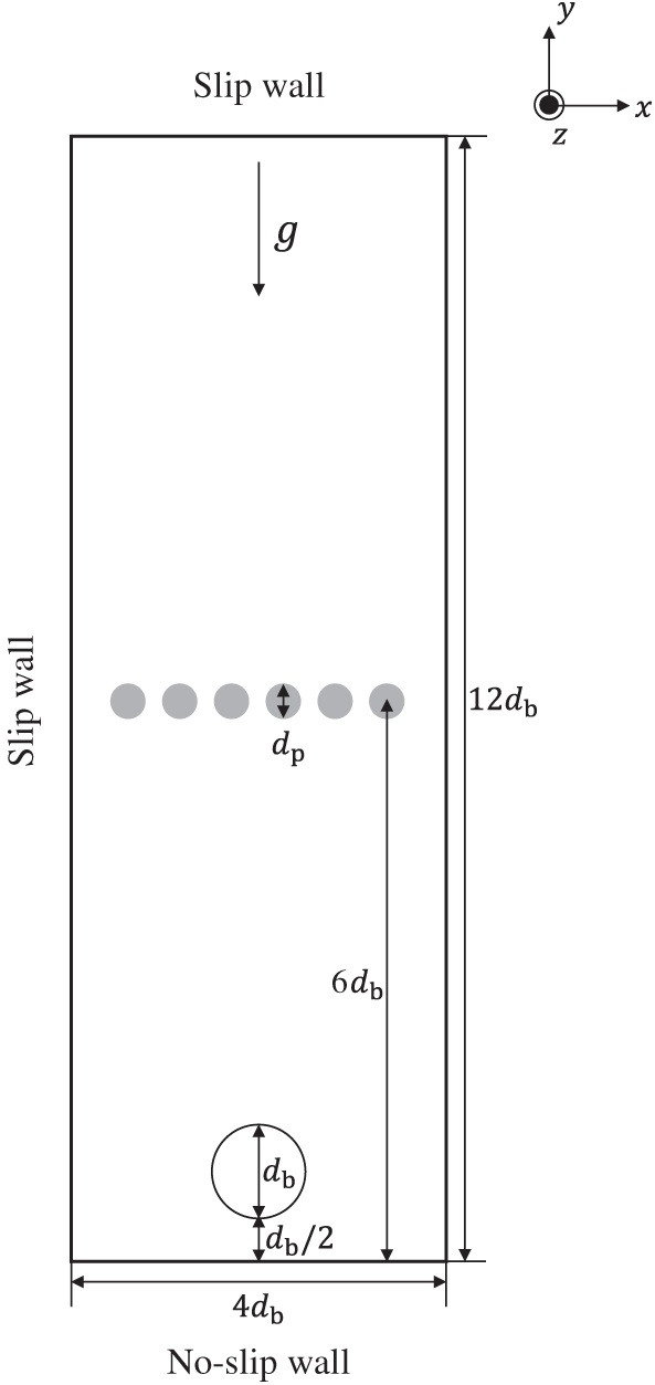
Figure 8: Computational setup for numerical simulations of a rising bubble moving through a layer of particles

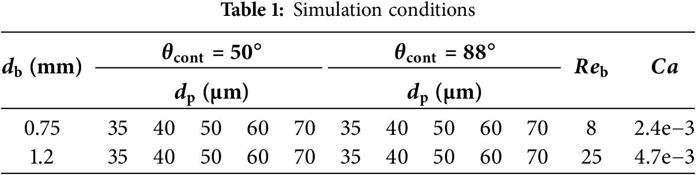
A stationary spherical bubble is initially placed at the center of the domain, positioned one bubble diameter db above the bottom wall. The initialization process is based on numerical integration of the implicit function developed by Bná et al. [45]. A total of 401 particles are uniformly distributed along the x-direction in the range of db⩽x⩽3db and located at the mid-plane of the yz-plane. The bubble reaches its terminal velocity before passing through the particle layer.

Before validating the present bubble-particle attachment algorithm, the terminal velocity of a rising bubble without particles is compared with the empirical relation given in Eq. (16). The terminal velocity, determined from the velocity of the bubble center, shows good agreement with the empirical value, as illustrated in Fig. 9.

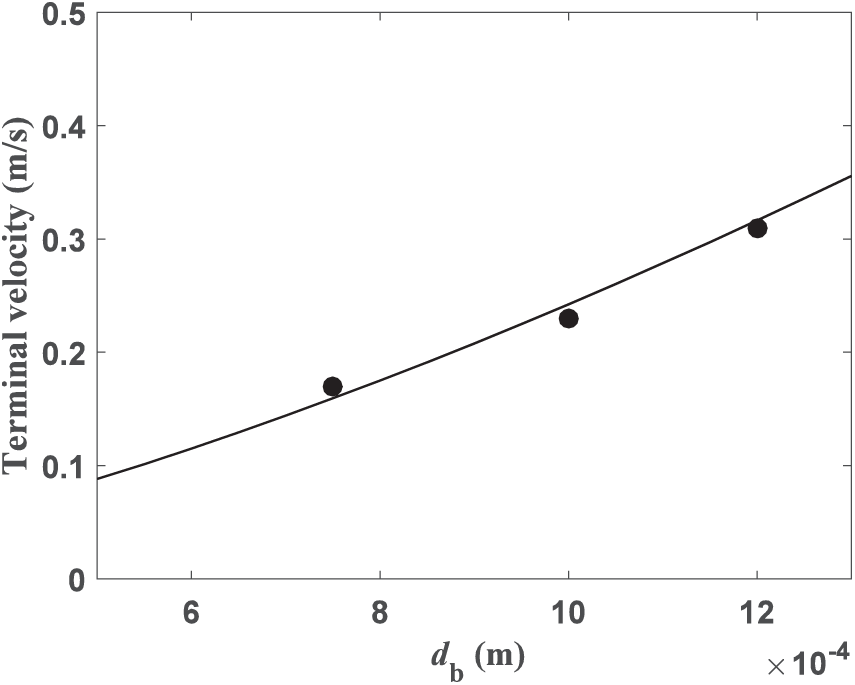
Figure 9: Terminal velocity of a rising bubble as a function of the bubble diameter db. —: empirical results from Eq. (16); ∙: the present simulation results for db of 0.75, 1.0, and 1.2 mm

5.1.1 Collision Probability and Collision Diameter

The collision probability (Eq. (12)) obtained from the present simulation is compared with that predicted by the theoretical relationship (Eq. (14)). To calculate the collision probability in the simulation, the ratio of the ideal to the actual number of colliding particles is required. From the definition in Section 3.2, the ideal number of colliding particles Nci is proportional to the square of the number of particles within the range 1.5db⩽x⩽2.5db. The actual number of colliding particles Ncr is proportional to the square of the total number of tagged particles identified as colliding. Fig. 10 shows the collision probability as a function of particle and bubble diameters. The simulation results are in good agreement with the theoretical predictions.

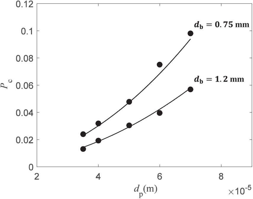
Figure 10: Collision probability Pc as a function of particle diameter dp for bubble diameters db of 0.75 and 1.2 mm. —: theoretical relationship (Eq. (14)); ∙: the present simulation results for dp of 35, 40, 50, 60, and 70 µm

The collision diameter dOC is further compared with results calculated using the model equation. From Eqs. (12) and (13), the square of the collision diameter is proportional to the total number of colliding particles. This length is obtained from Eq. (13) as dOC=dbPc. Fig. 11 shows the collision diameter as a function of particle and bubble diameters. The collision diameter dOC is linearly proportional to the particle diameter dp, implying that the total number of colliding particle is proportional to the square of the particle diameter dp.

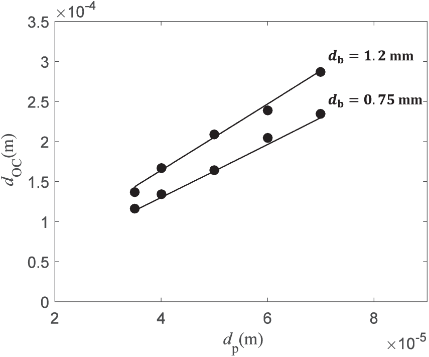
Figure 11: Collision diameter dOC as a function of the particle diameter dp for bubble diameters db of 0.75 and 1.2 mm. —: theoretical relationship from Eqs. (13) and (14); ∙: simulation results for particle diameters dp of 35, 40, 50, 60, and 70 µm

5.1.2 Attachment Probability and Attachment Diameter

The attachment probability and attachment diameter are compared with theoretical and experimental results [44]. In the present simulation, the attachment probability is estimated using Eq. (18). The total number of attached particles Na is obtained by squaring the total number of eliminated particles. Fig. 12 shows the attachment probability as a function of particle diameter, bubble diameter, and contact angle. The simulation results are in favorable agreement with experimental data, with the maximum errors within 5%.

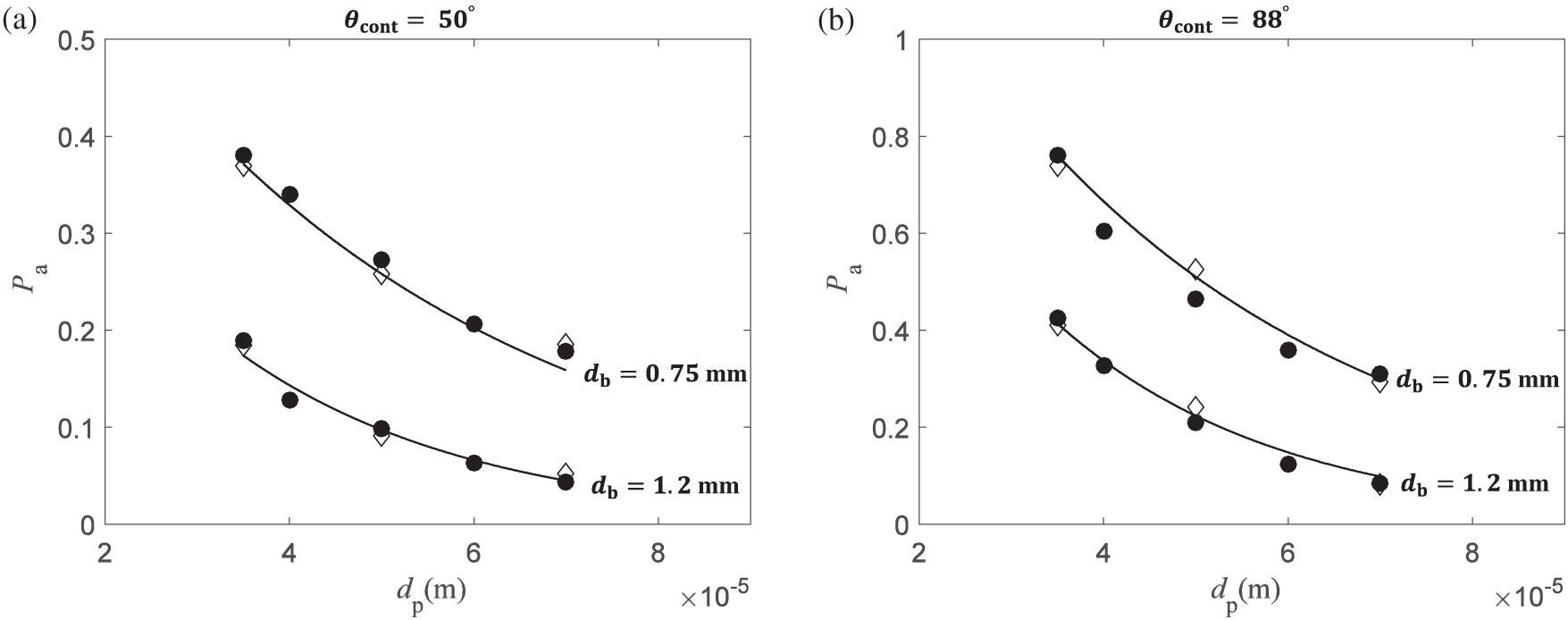
Figure 12: Attachment probability Pa as a function of particle diameter dp and bubble diameter. Bubble diameters db of 0.75 and 1.2 mm are considered for contact angles θcont of (a) 50∘ and (b) 88∘. Symbols are results for particle diameters dp of 35,40,50,60, and 70 µm. —: fitting results from Eqs. (20) and (21); ◊: experimental results [44]; ∙: the present simulations results

The attachment diameter is calculated as dOA=dOCPa=dbPcPa using Eqs. (13) and (19). The square of the attachment diameter represents the total number of attached particles. Fig. 13 shows the attachment diameter as a function of particle diameter, bubble diameter, and contact angle. Overall, the present simulation results agree well with theoretical [27] and experimental results [44]. For a bubble diameter of 0.75 mm, the attachment diameter dOA increases with particle diameter dp. In contrast, for a bubble diameter of 1.2 mm, the attachment diameter is less sensitive to changes in the particle diameter dp.

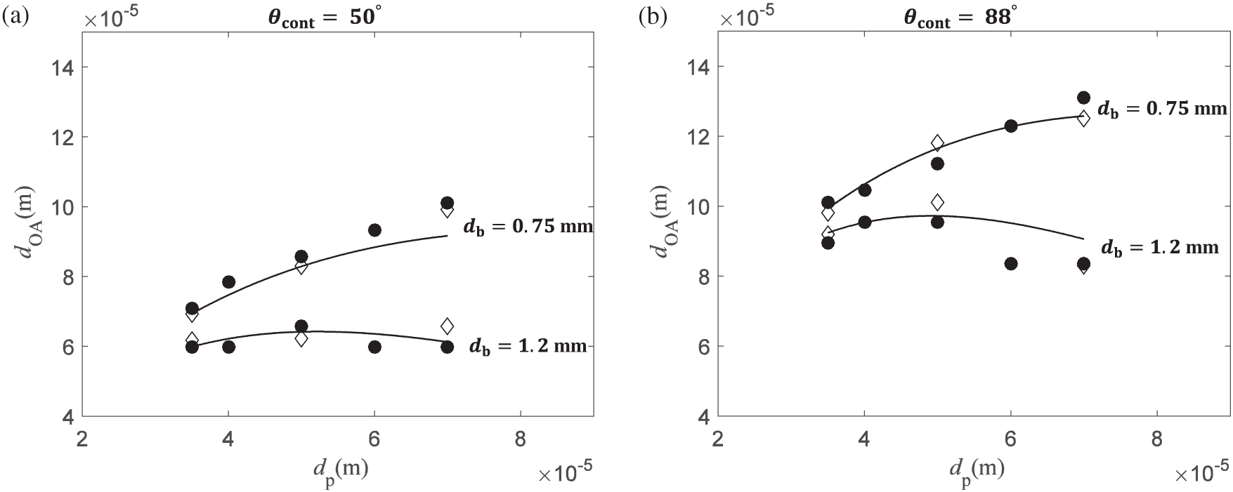
Figure 13: Attachment diameter dOA as a function of particle diameter dp and bubble diameter. Bubble diameters db of 0.75 and 1.2 mm are considered for contact angles θcont of (a) 50∘ and (b) 88∘. Symbols are results of the particle diameters dp of 35, 40, 50, 60, and 70 µm. —: theoretical results [27]; ◊: experimental results [44]; ∙: the present simulations results

This tendency arises from the product of the collision probability and the attachment probability:

P=PcPa=NcrNciNaNcr=NaNci=(sin⁡θcr)2,(29)

where P is referred to as the flotation probability [27] or total attachment probability [2]. The probability corresponds to the ratio of attached particles to the ideal number of colliding particles. The relation indicates that the attachment diameter dOA is proportional to sin⁡θcr when the bubble diameter db is fixed. The theoretical results in Fig. 13 are obtained from dbP. The attachment diameter dOA also increases with the contact angle θcont, since a larger θcont increases the attachment probability Pa (Fig. 12).

5.1.3 Visualization Results

The present method distinguishes between sliding or attachment of colliding particles, thereby enabling observation of particle motions near the bubble surface, as shown in Figs. 14 and 15. Bubbles are represented by iso-surfaces of the volume fraction c=0.5. Particles near the bubble are visualized both with and without the numerical model for bubble-particle attachment. Without the model, no particles interact with the bubble, as shown in Figs. 14a and 15a. In this case, particles remain even when in contact with the bubble surface, whereas with the model, attached particles are eliminated.

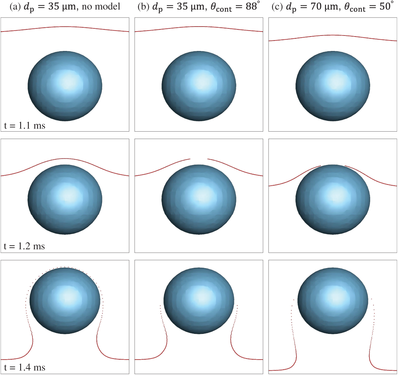
Figure 14: Visualization of a layer of particles interacting with a bubble with db of 0.75 mm under three conditions: (a) dp=35 µm, without the bubble-particle attachment model; (b) dp=35 µm, with the bubble-particle attachment model and θcont=88∘; (c) dp=70 µm, with the bubble-particle attachment model and θcont=50∘

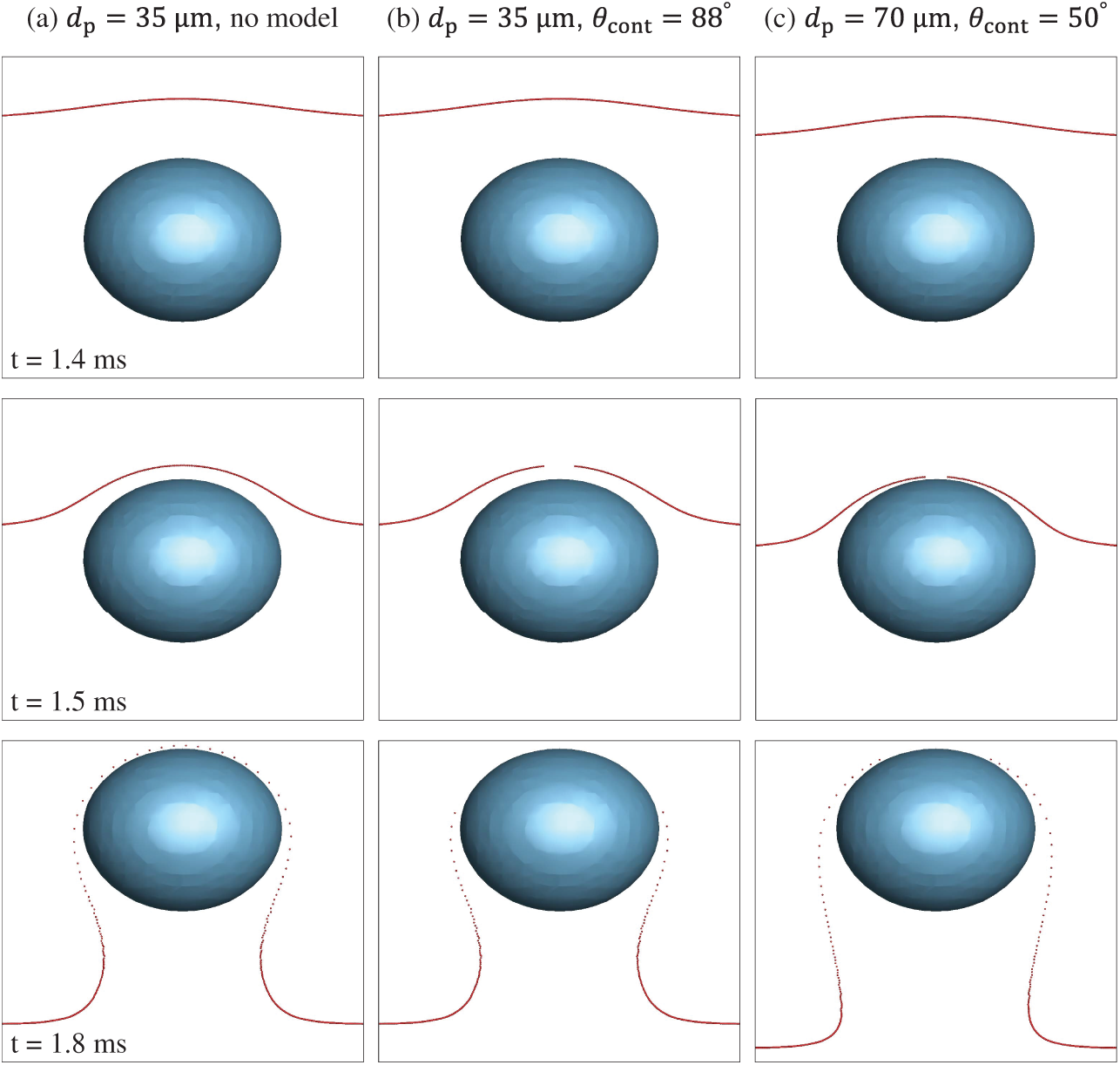
Figure 15: Visualization of a layer of particles interacting with a bubble with db of 1.2 mm under three conditions: (a) dp=35 µm, without the bubble-particle attachment model; (b) dp=35 µm, with the bubble-particle attachment model and θcont=88∘; (c) dp=70 µm, with the bubble-particle attachment model and θcont=50∘

As discussed in Section 4.5, attached particles are eliminated on the effective bubble before making contact with the actual bubble surface. The bubble surface is reconstructed from the VOF method in an Eulerian framework, while the particle size is smaller than the grid size, making the prediction of the exact collision location difficult. Therefore, sliding and attachment are determined on the effective bubble surface, which is larger than the actual bubble. For the bubble with a diameter of 0.75 mm, the number of attached particles is nearly identical for both θcont of 50∘ and 88∘, as shown in Fig. 14b and 14c. This is because both cases yield similar attachment diameters of about 0.1 mm (Fig. 13a and 13b).

Similarly, Fig. 15 shows the case of a bubble with diameter 1.2 mm. The number of attached particles in Fig. 15b is greater than in Fig. 15c, because the attachment diameter in the former case is 90 µm, compared to 60 µm in the latter case (see Fig. 13c and 13d). In this study, both the bubble and the particle are initially approximated as spheres. However, the models require the bubble–particle angle and bubble radius to be defined based on the effective bubble, determined from the surface normal vector. Consequently, an ellipsoidal bubble shape can also be treated. The simulation results in Fig. 15 show that spherical bubbles gradually transform into ellipsoidal shapes as they rise in the bath.

5.2 Multiple Rising Bubbles through a Layer of Particles

The present bubble-particle attachment method can be extended to interactions involving multiple bubbles and particles. The computational domain is the same as in the single bubble case presented in Section 5.1, except that periodic boundary conditions are applied to the side walls instead of slip conditions. Fig. 16 shows 3×3 stationary spherical bubbles of diameter 0.75 mm, initialized at equal distances from the bottom wall. Particles of diameter 35 µm are uniformly distributed above the bubbles along the x-axis at the middle of the yz-plane. Two cases are simulated: with and without the bubble–particle attachment model.

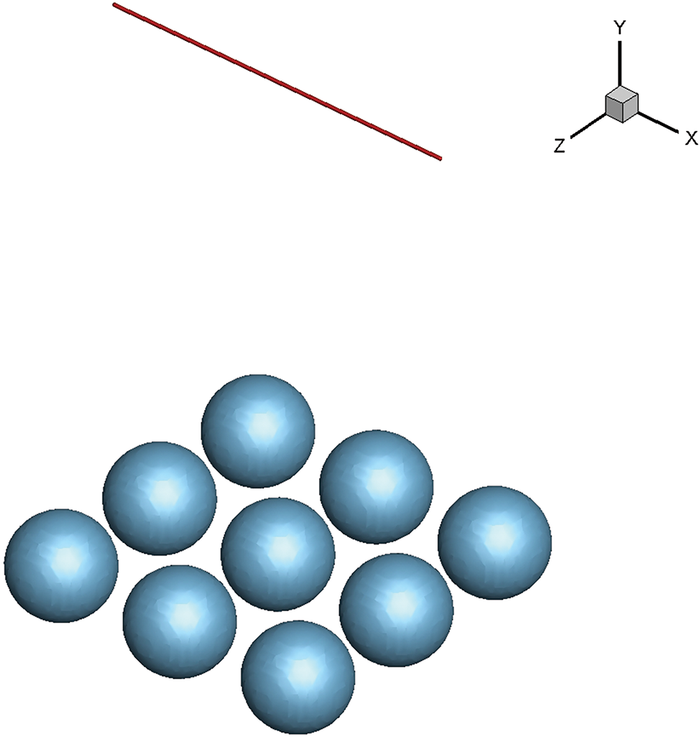
Figure 16: Initial configuration of multiple bubbles and a layer of particles. db of 0.75 mm and dp of 35 µm are considered

For the multiple-bubble case, tilt and side views are visualized to illustrate interactions between bubbles and a layer of particles, as shown in Figs. 17 and 18. Without the attachment model, no particles adhere to the bubble surface as shown in Figs. 17a and 18a. In contrast, with the attachment model, attached particles are eliminated on the bubble surface as shown in Figs. 17b and 18b.

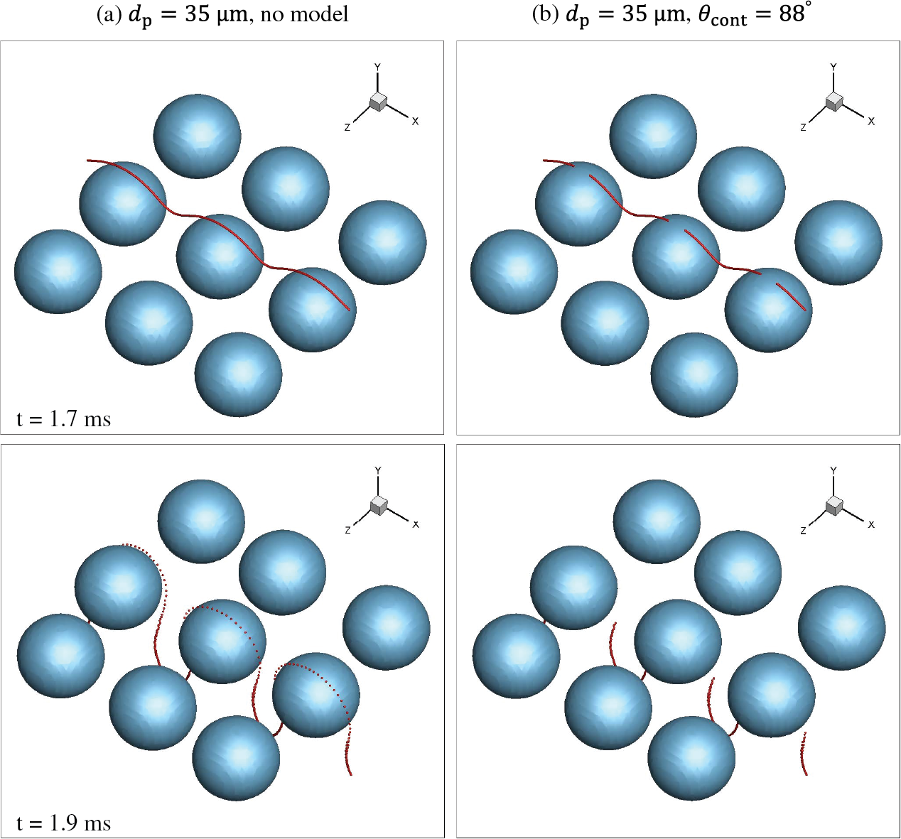
Figure 17: Multiple rising bubbles through a layer of particles. (a) Without the attachment model and (b) with the attachment model. db=0.75 mm, dp=35 µm, and θcont=88∘

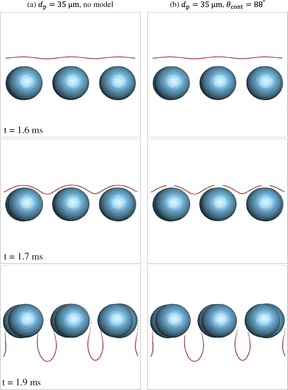
Figure 18: Side views (xy-plane) of multiple rising bubbles through a layer of particles (a) without the attachment model and (b) with the attachment model. db=0.75 mm, dp=35 µm, and θcont=88∘

6  Conclusion

A numerical method for simulating gas-liquid-solid flows, including bubble-particle attachment, has been developed. Phase interfaces are described and advected using a geometrical conserving VOF method, while particle dynamics are solved in a Lagrangian framework. The bubble–particle attachment is modeled in the VOF framework using the concept of an effective bubble together with the theoretical relationships of Nguyen et al. [27].

The present numerical method consists of two steps: collision detection and sliding/attachment determination during bubble-particle interaction. It requires evaluation of the angle between two vectors: the bubble velocity vector and the vector of the particle position relative to the bubble center. A method for calculating this angle in the geometric VOF framework is proposed. Since the exact collision location cannot be easily resolved in the VOF framework, collisions are defined to occur when a particle lies between the surfaces of the actual bubble and an effective bubble with a larger radius, introduced to account for grid-resolution limits.

The present numerical method has been validated by reproducing experimental cases. Simulations of a rising bubble moving through a layer of particles, for a range of bubble diameters, particle diameters, and contact angles, demonstrated that the present numerical method accurately predicts collision and attachment probabilities. The efficacy of the present attachment model is further confirmed through visualizations of the simulated particle dynamics. Finally, the applicability of the present method to complex industrial problems has been illustrated by simulating multiple rising bubbles interacting with a layer of many particles.

The present numerical method successfully simulates bubble-particle attachment, yet several limitations remain. First, because it relies on the concept of an effective bubble and grid resolution, the precise collision location and the detailed physics of liquid film formation and rupture are simplified. Second, complex physical factors such as particle hydrophobicity/hydrophilicity, surface roughness, and turbulent flow conditions are not fully considered. Future work should therefore aim to incorporate more detailed models, such as molecular dynamics or continuum-scale coupling, to better capture film physics.

Acknowledgement: The authors gratefully acknowledge Sanghyun Ha and Jeongbo Shim for their constructive comments on this work.

Funding Statement: The work was supported by the National Research Foundation of Korea (NRF) under the Grant Numbers NRF-2021R1A2C2092146 and RS-2023-00282764.

Author Contributions: The authors confirm contribution to the paper as follows: Conceptualization, Hojun Moon and Donghyun You; methodology, Hojun Moon; software, Hojun Moon; validation, Hojun Moon; formal analysis, Hojun Moon; investigation, Hojun Moon and Donghyun You; resources, Donghyun You; data curation, Hojun Moon; writing—original draft preparation, Hojun Moon; writing—review and editing, Donghyun You; visualization, Hojun Moon; supervision, Donghyun You; project administration, Donghyun You; funding acquisition, Donghyun You. All authors reviewed the results and approved the final version of the manuscript.

Availability of Data and Materials: All data generated or analyzed during this study are included in this published article.

Ethics Approval: Not applicable.

Conflicts of Interest: The authors declare no conflicts of interest to report regarding the present study.

Appendix A Tuning of the Effective Collision Angle and the Critical Angle

In the present numerical method, collisions are defined using both the actual and effective bubble surfaces. The effective collision angle θm∗ and critical angle θcr∗ must be modeled from the actual collision angle θm and critical angle θcr. Eqs. (25a) and (25b) serve as tuning relations. Parametric studies show that the effectiveness factors km and kcr vary linearly with the particle diameter dp. Accordingly, the effectiveness factors km and kcr are expressed as follows:

km=fm×dp+gm,(A1a)

kcr=fcr×dp+gcr,(A1b)

where fm and gm are functions of the bubble diameter db; and fcr and gcr are functions of the bubble diameter db and contact angle θcont, respectively:

fm=a1×db+a2,(A2a)

gm=a3×db+a4,(A2b)

fcr=b1×db+b2×sin⁡(θcont/2)+b3×db×sin⁡(θcont/2)+b4,(A2c)

gcr=b5×db+b6×sin⁡(θcont/2)+b7×db×sin⁡(θcont/2)+b8,(A2d)

where the coefficients ai for i=[1,4] and bi for i=[1,8] are constants to be determined. The contact angle θcont is expressed in a sinusoidal form, similar to Eq. (20). The collision angle θm is not a function of contact angle θcont as shown in Eqs. (13) and (14). Therefore, fm and gm depend only on the bubble diameter db.

The coefficients in Eqs. (A1) and (A2) are determined as follows. First, the effectiveness factors km and kcr are obtained by adjusting their values until the collision and attachment probabilities from the simulation agree with those from Eqs. (14) and (20). The effectiveness factors are then linearly fitted to obtain fm, fcr, gm, and gcr. Coefficients ai and bi can be determined by substituting bubble diameters and contact angles into Eqs. (A2a) to (A2d). This tuning process must be repeated, and the coefficients recalibrated, if the size of the effective bubble is changed.

References

1. Nguyen AV, Schulze HJ. Colloidal science of flotation. Vol. 118. In: Surfactant sciences series. 1st ed. Boca Raton, FL, USA: CRC Press; 2003. [Google Scholar]

2. Zhang L, Taniguchi S. Fundamentals of inclusion removal from liquid steel by bubble flotation. Int Mater Rev. 2000;45(2):59–82. doi:10.1179/095066000101528313. [Google Scholar] [CrossRef]

3. Evans LF. Bubble-mineral attachment in flotation. Ind Eng Chem. 1954;46(11):2420–4. [Google Scholar]

4. Dobby GS, Finch JA. A model of particle sliding time for flotation size bubbles. J Colloid Interface Sci. 1986;109(2):493–8. doi:10.1016/0021-9797(86)90327-9. [Google Scholar] [CrossRef]

5. Dobby GS, Finch JA. Particle size dependence in flotation derived from a fundamental model of the capture process. Int J Miner Process. 1987;21(3–4):241–60. doi:10.1016/0301-7516(87)90057-3. [Google Scholar] [CrossRef]

6. Sutherland KL. Physical chemistry of flotation. XI. Kinetics of the flotation process. J Phys Chem. 1948;52(2):394–425. doi:10.1021/j150458a013. [Google Scholar] [PubMed] [CrossRef]

7. Liu L, Zhan M, Wang R, Liu Y. Three-dimensional VOF-DEM simulation study of particle fluidization induced by bubbling flow. Processes. 2024;12(6):1053. doi:10.3390/pr12061053. [Google Scholar] [CrossRef]

8. Li X, Hao Y, Zhao P, Fan M, Song S. Simulation study on the phase holdup characteristics of the gas–liquid-solid mini-fluidized beds with bubbling flow. Chem Eng J. 2022;427(31):131488. doi:10.1016/j.cej.2021.131488. [Google Scholar] [CrossRef]

9. Wang H, Yan X, Li D, Zhou R, Wang L, Zhang H, et al. Recent advances in computational fluid dynamics simulation of flotation: a review. Asia Pac J Chem Eng. 2021;16(5):e2704. doi:10.1002/apj.2704. [Google Scholar] [CrossRef]

10. Chan TTK, Ng CS, Krug D. Bubble–particle collisions in turbulence: insights from point-particle simulations. J Fluid Mech. 2023;959:A6. doi:10.1017/jfm.2025.10405. [Google Scholar] [CrossRef]

11. Zheng K, Yan X, Wang L, Zhang H. Predictions of particle–bubble collision efficiency and critical collision angle in froth flotation. Colloids Surf A Physicochem Eng Asp. 2024;702(Part 1):134985. doi:10.1016/j.colsurfa.2024.134985. [Google Scholar] [CrossRef]

12. Szmigiel A, Apel DB, Skrzypkowski K, Wojtecki L, Pu Y. Advancements in machine learning for optimal performance in flotation processes: a review. Minerals. 2024;14(4):331. doi:10.3390/min14040331. [Google Scholar] [CrossRef]

13. Maxwell R, Ata S, Wanless EJ, Moreno-Atanasio R. Computer simulations of particle–bubble interactions and particle sliding using discrete element method. J Colloid Interface Sci. 2012;381(1):1–10. doi:10.1016/j.jcis.2012.05.021. [Google Scholar] [PubMed] [CrossRef]

14. Moreno-Atanasio R. Influence of the hydrophobic force model on the capture of particles by bubbles: a computational study using discrete element method. Adv Powder Technol. 2013;24(4):786–95. doi:10.1016/j.apt.2013.05.001. [Google Scholar] [CrossRef]

15. Moreno-Atanasio R, Gao Y, Neville F, Evans GM, Wanless EJ. Computational analysis of the selective capture of binary mixtures of particles by a bubble in quiescent and fluid flow. Chem Eng Res Des. 2016;109:354–65. doi:10.1016/j.cherd.2016.01.035. [Google Scholar] [CrossRef]

16. Sarrot V, Guiraud P, Legendre D. Determination of the collision frequency between bubbles and particles in flotation. Chem Eng Sci. 2005;60(22):6107–17. doi:10.1016/j.ces.2005.02.018. [Google Scholar] [CrossRef]

17. Nadeem M, Ahmed J, Chughtai IR, Ullah A. CFD-based estimation of collision probabilities between fine particles and bubbles having intermediate reynolds number. The Nucleus. 2009;46(3):153–9. doi:10.71330/nucleus.46.03.940. [Google Scholar] [CrossRef]

18. Koh PTL, Schwarz MP. CFD modelling of bubble–particle collision rates and efficiencies in a flotation cell. Miner Eng. 2003;16(11):1055–9. doi:10.1016/j.mineng.2003.05.005. [Google Scholar] [CrossRef]

19. Koh PTL, Schwarz MP. CFD modelling of bubble–particle attachments in flotation cells. Miner Eng. 2006;19(6–8):619–26. doi:10.1016/j.mineng.2005.09.013. [Google Scholar] [CrossRef]

20. Li Y, Zhang J, Fan LS. Numerical simulation of gas–liquid–solid fluidization systems using a combined CFD-VOF-DPM method: bubble wake behavior. Chem Eng Sci. 1999;54(21):5101–7. doi:10.1016/s0009-2509(99)00263-8. [Google Scholar] [CrossRef]

21. Chen C, Fan LS. Discrete simulation of gas-liquid bubble columns and gas-liquid-solid fluidized beds. AIChE J. 2004;50(2):288–301. doi:10.1002/aic.10027. [Google Scholar] [CrossRef]

22. Xu Y, Ersson M, Jönsson PG. A numerical study about the influence of a bubble wake flow on the removal of inclusions. ISIJ Int. 2016;56(11):1982–8. doi:10.2355/isijinternational.isijint-2016-249. [Google Scholar] [CrossRef]

23. Pozzetti G, Peters B. A multiscale DEM-VOF method for the simulation of three-phase flows. Int J Multiphase Flow. 2018;99(15):186–204. doi:10.1016/j.ijmultiphaseflow.2017.10.008. [Google Scholar] [CrossRef]

24. Zhao N, Wang B, Kang Q, Wang J. Effects of settling particles on the bubble formation in a gas-liquid-solid flow system studied through a coupled numerical method. Phys Rev Fluids. 2020;5(3):033602. doi:10.1103/physrevfluids.5.033602. [Google Scholar] [CrossRef]

25. Teran LA, Rodriguez SA, Laín S, Jung S. Interaction of particles with a cavitation bubble near a solid wall. Phys Fluids. 2018;30(12):123304. doi:10.1063/1.5063472. [Google Scholar] [CrossRef]

26. Liu H, Tang J, Sun L, Mo Z, Xie G. An assessment and analysis of phase change models for the simulation of vapor bubble condensation. Int J Heat Mass Transf. 2020;157(Part A):119924. doi:10.1016/j.ijheatmasstransfer.2020.119924. [Google Scholar] [CrossRef]

27. Nguyen AV, Ralston J, Schulze HJ. On modelling of bubble–particle attachment probability in flotation. Int J Miner Process. 1998;53(4):225–49. doi:10.1016/s0301-7516(97)00073-2. [Google Scholar] [CrossRef]

28. Lecrivain G, Yamamoto R, Hampel U, Taniguchi T. Direct numerical simulation of a particle attachment to an immersed bubble. Phys Fluids. 2016;28(8):083301. doi:10.1063/1.4960627. [Google Scholar] [CrossRef]

29. Moon H, Hong S, You D. Application of the parallel diagonal dominant algorithm for the incompressible Navier-Stokes equations. J Comput Phys. 2020;423(2):109795. doi:10.1016/j.jcp.2020.109795. [Google Scholar] [CrossRef]

30. Kim J, Moin P. Application of a fractional-step method to incompressible Navier-Stokes equations. J Comput Phys. 1985;59(2):308–23. doi:10.1016/0021-9991(85)90148-2. [Google Scholar] [CrossRef]

31. Henson VE, Yang UM. BoomerAMG: a parallel algebraic multigrid solver and preconditioner. Appl Numer Math. 2002;41(1):155–77. doi:10.1016/s0168-9274(01)00115-5. [Google Scholar] [CrossRef]

32. Crowe CT, Schwarzkopf JD, Sommerfeld M, Tsuji Y. Multiphase flows with droplets and particles. Boca Raton, FL, USA: CRC Press; 2011. [Google Scholar]

33. Scardovelli R, Zaleski S. Direct numerical simulation of free-surface and interfacial flow. Annu Rev Fluid Mech. 1999;31(1):567–603. doi:10.1146/annurev.fluid.31.1.567. [Google Scholar] [CrossRef]

34. Aulisa E, Manservisi S, Scardovelli R, Zaleski S. Interface reconstruction with least-squares fit and split advection in three-dimensional Cartesian geometry. J Comput Phys. 2007;225(2):2301–19. doi:10.1016/j.jcp.2007.03.015. [Google Scholar] [CrossRef]

35. Scardovelli R, Zaleski S. Analytical relations connecting linear interfaces and volume fractions in rectangular grids. J Comput Phys. 2000;164(1):228–37. doi:10.1006/jcph.2000.6567. [Google Scholar] [CrossRef]

36. Weymouth GD, Yue DKP. Conservative volume-of-fluid method for free-surface simulations on Cartesian-grids. J Comput Phys. 2010;229(8):2853–65. doi:10.1016/j.jcp.2009.12.018. [Google Scholar] [CrossRef]

37. Brackbill JU, Kothe DB, Zemach C. A continuum method for modeling surface tension. J Comput Phys. 1992;100(2):335–54. doi:10.1016/0021-9991(92)90240-y. [Google Scholar] [CrossRef]

38. Popinet S. An accurate adaptive solver for surface-tension-driven interfacial flows. J Comput Phys. 2009;228(16):5838–66. doi:10.1016/j.jcp.2009.04.042. [Google Scholar] [CrossRef]

39. Francois MM, Cummins SJ, Dendy ED, Kothe DB, Sicilian JM, Williams MW. A balanced-force algorithm for continuous and sharp interfacial surface tension models within a volume tracking framework. J Comput Phys. 2006;213(1):141–73. doi:10.1016/j.jcp.2005.08.004. [Google Scholar] [CrossRef]

40. Nguyen AV. New method and equations for determining attachment tenacity and particle size limit in flotation. Int J Miner Process. 2003;68(1–4):167–82. doi:10.1016/s0301-7516(02)00069-8. [Google Scholar] [CrossRef]

41. Nguyen AV. The collision between fine particles and single air bubbles in flotation. J Colloid Interface Sci. 1994;162(1):123–8. doi:10.1006/jcis.1994.1016. [Google Scholar] [CrossRef]

42. Clift R, Grace JR, Weber ME. Bubbles, drops, and particles. New York, NY, USA: Academic Press; 1978. [Google Scholar]

43. Oeters F. Metallurgy of steelmaking. 1st ed. Düsseldorf, Germany: Verlag Stahleisen; 1994. [Google Scholar]

44. Hewitt D, Fornasiero D, Ralston J. Bubble–particle attachment. J Chem Soc Faraday Trans. 1995;91(13):1997–2001. doi:10.1039/ft9959101997. [Google Scholar] [CrossRef]

45. Bná S, Manservisi S, Scardovelli R, Yecko P, Zaleski S. Numerical integration of implicit functions for the initialization of the VOF function. Comput Fluids. 2015;113:42–52. [Google Scholar]