Detecting Vehicle Mechanical Defects Using an Ensemble Deep Learning Model with Mel Frequency Cepstral Coefficients from Acoustic Data

1  Introduction

Recently, a surge has been observed in research on the automated recognition of sound, gaining traction across various interdisciplinary domains such as multimedia, bio-acoustics monitoring, anomaly detection, and environmental sound analysis [1], etc. Three specific stages address the problem of sound classification: extracting specific features, signal preprocessing, and their subsequent classification. Signal processing involves breaking down the input signal into its parts, which are then used to extract characteristics that work well together. To express complicated information as a feature vector and reduce the quantity of data, feature extraction is essential [2]. Aspects such as frame features, crossing rate, and pitch, commonly engaged in speech recognition applications, have been exposed to classification using diverse models like long short-term memory (LSTMs) and convolutional neural networks (CNNs). Recently, linear prediction coefficients, stabilized auditory images, and spectrogram image features have been widely used [2]. Additionally, the performance of audio signals classification has significantly improved as a result of the integration of many soft computing and machine learning (ML) techniques, including multi-layer perceptrons, random forest (RF), and deep learning approaches [3].

Spectrogram image features yield more precise outcomes by capturing sound waves in situations involving noisy data. These waves make up expanding areas of low and high pressure. The distinctive patterns formed by these high and low-pressure regions are unique to various sounds [4]. These waves exhibit specific attributes, including wavelength, wave speed, frequency, and time period. Such attributes play an essential role in categorizing sound, mirroring the way humans classify them. In essence, a spectrogram is an optical depiction of the frequency spectrogram implicit in a sound wave [5]. The spectrogram exhibits low frequency, which causes strong contents in the upper area and intense noise excitation in the lower half. These images from the spectrogram can be effectively employed in conjunction with various ML classifiers [6]. The authors proposed an integrated technique that combines an ML model with a deep learning (DL) autoencoder for the detection of abstruse illustration through unsupervised learning [7]. The proposed method utilizes spectrogram images as visual representations of the frequency spectrum of a signal. Sound signals, characterized by infrequency, weak locality, and diverse pattern illustration in the spectrogram, pose unique challenges for analysis.

Anomaly detection stands out as a primary application of ML in various industries, finding utility in video surveillance, critical infrastructure monitoring, and the identification of fraudulent activities. However, predominant approaches focus on identifying anomalies. Challenges emerge when the entire environment cannot be fully covered, resulting in blind spots where predictions can not be made [8]. This limitation is particularly pertinent to the internal areas in industrial premises. Visual inspections may fail to capture the true condition of the monitored entity; for instance, a pump with a minor leakage, an ungreased slide rail, or a fan experiencing voltage fluctuations may appear visually intact but reveal their actual conditions through distinctive sound patterns when monitored acoustically [9]. Additionally, audio consideration holds benefits of being cost-effective and efficiently portable with simple hardware [10]. Detecting machinery malfunctions early using an audio anomaly detection system can avoid more significant indemnity and lead to reduced improvement and conservation costs.

The problem at hand involves the challenge of accurately classifying sounds in diverse and dynamic environments, spanning applications like speech recognition, environmental monitoring, and audio surveillance. Utilizing DL methods is highly valuable for classifying the diverse sounds present in the surrounding environment. The primary focus lies in different machine sounds utilized to identify anomalies. Distortions in acoustic sources, along with the presence of noise, pose challenges due to their representation as waves and amplitudes, making comprehension challenging within various frameworks. Additionally, the system must contend with a vast amount of audio files and recordings, further complicated by the amalgamation of some files, rendering the identification and segregation processes more intricate. As a result, for effective sound classification, DL methods are essential.

This work uses DL techniques to develop an advanced audio classification system. Managing the audio data and developing a model that can reliably categorize a large range of sounds is the primary challenge. The main goal is to improve accuracy and offer effective user assistance by utilizing the developments in DL, particularly in the areas of speaker identification and recognition. The audio samples are first put through a rigorous preprocessing procedure that focuses on extracting the Mel-Frequency Cepstral Coefficients (MFCCs) characteristics from each audio signal. To preserve the distinctive characteristics of the audio data and prepare it for a more thorough analysis, the second step is essential. The DL model is then built using the retrieved MFCC feature vectors. Using a DL model increases the system’s capacity to identify complex auditory patterns, which improves the classification accuracy of sounds. In addition to accurately classifying audio signals, this methodical technique aims to provide users with a sophisticated tool for effectively analyzing and identifying sounds. The following are the main contributions of the proposed approach.

•   The study introduces a DL-based technique that uses the collected acoustic data to precisely identify vehicle malfunctions. For this purpose, important characteristics of the audio signal are extracted using MFCC features of normal and anomalous voices.

•   The study introduces an ensemble model by incorporating the capabilities of LeNet and a hierarchical attention mechanism (HAM) model for the accurate classification of diverse defects based on sounds. MFCC features extracted from sound are utilized as input features for DL models.

•   Various DL models are applied, including LSTM, bidirectional LSTM (BiLSTM), convolutional recurrent neural network (CRNN), CNN, gated recurrent unit (GRU), attention mechanism model (AM), capsule network model (CNM), ResNet, EfficientNet, and HAM for comprehensive evaluation.

•   A thorough evaluation is conducted using various metrics. In addition, results from k-fold cross-validation and comparison with approaches from previous studies further highlight the effectiveness of the proposed strategy. Additionally, the receiver operating characteristic area under the curve (ROC-AUC) and precision-recall (PR-AUC) measures are used to assess the model’s discriminative ability. Furthermore, a performance comparison with the most advanced models is conducted.

Further, Section 2 discusses the relevant literature on audio classification. Section 3 describes the proposed approach, dataset, and models. Section 4 discusses the results and discussion based on the proposed methodology. Lastly, Section 5 provides the conclusion of this research.

2  Related Work

Deep auto encoders (AE) are used in many applications for anomalous sound detection [11]. The study [12] reconstructs Mel-spectrograms using a convolutional AE to find abnormalities in industrial facilities. The authors combine more than one spectrogram frame to feed into an AE with dense connections. In this case, anomalous sound detection (ASD) is seen as a statistical hypothesis test. The finding that edge frames are typically more difficult to reconstruct, particularly when working with non-stationary sounds, is the basis for this hypothesis [13]. Reconstructing auditory spectrum characteristics requires knowledge of a sequence-to-sequence network and the sequential character of sound designs [14]. Another possibility is to use a slightly different strategy where ASD is achieved by using an ensemble of AEs. To preprocess the data, a variety of acoustic front-end techniques are used for denoising and reverberation because AEs are relieved of the task of recreating noise, and performance is improved [15].

SNIPER is a unique approach that allows finding abnormalities without requiring a system-wide retraining [16]. A new detector having a true positive rate (TPR) of 1 for that particular anomaly is cascaded for every ignored abnormality. To compute the TPR, samples of the observed anomaly are created using a generative model. A few direct waveform-based ASD techniques have been developed in addition to spectrogram-based alternatives in [17] and [18]. These methods are based on autoregressive models that use causal dilated convolutions to predict the next sample and use prediction error to measure irregularity [19].

Environmental sound recognition (ESR) has attracted a lot of interest lately, with an emphasis on using DL techniques to improve performance. DL has been utilized in earlier research to investigate different methods for sound recognition [20]. Spectrograms can be used as input to CNN and artificial neural networks (ANNs), whereas other models take the raw waveform in its unaltered state [21]. Here, a CNN-based wireless sensor network (WSN) using Raspberry Pi nodes is suggested for sound classification. The Raspberry Pi devices were used to encrypt the audio, which was then sent for classification. Since the embedded system has the processing capacity to accomplish these operations, it was shown to be capable of sound categorization and feature extraction [22]. A Raspberry Pi was used to evaluate the classification time and accuracy of many conventional ML approaches. By using a multi-stage hierarchical method for audio classification, the authors offered an adaptable solution. This method can choose the best classifiers at every stage while taking running time, audio kind, and power consumption into account [23]. When using the ESC dataset, CNN applications for ESR attracted a lot of interest as a standard for evaluating the performance of more modern networks [24]. The benefits and viability of incorporating an ML approach for accurate classification, however, are not well discussed [25]. The study [26] suggested a method for classification of urban noises in the context of the Internet of Things (IoT) using a CNN model, made especially for use with an RPi 4. The model used feature maps from spectrograms and 2D convolutions as input for classification. In a similar vein, the study [27] presented and assessed an embedded solution for low-power microcontroller sound classification that used CNNs and spectrogram inputs. To determine the trade-off between memory, CPU, and accuracy utilization on the microcontroller, many CNN designs were assessed. Moreover, the temporal summary is missing, which shows how lightweight CNNs may accomplish the highest accuracy even on embedded devices with limited resources.

A temporal frequently attention-based CNN model (TFCNN) is used with long-Mel spectrograms, characteristics for efficiently learning time and frequency. The authors experimented to test how a particular spectrogram frequency band affects the model’s categorization to confirm the effectiveness of the proposed approach. Various hardware have also been studied to enhance the achievement of DL inference for audio applications [28]. The study looks at a suitable method for multiclass damage localization that can be harmful. To improve the classification outcomes, a unique majority voting method utilizing a global CNN-1D model is also used [29]. Supervised learning and unsupervised learning are the two basic methods utilized for AD using DL. In order to establish normal and abnormal classifications, a balanced preparation of the data labeled in each condition is required [30–32]. Several research works have used DL models like CNN to handle the challenges of classifying each state. These studies used the assumption that the data for all states were adequately protected [33]. The study used Naïve Bayes to classify vectors of auditory features. Another work utilized the K-means approach to create a balanced dataset and label test data from many flight tests as normal and abnormal [34]. Then, using the same dataset, the linear regression model was used to categorize states in real time.

Reconstruction mistakes have been used in many research works [35–37] to categorize aberrant states and separate them from normal states. Although it is less accurate than error prediction approaches, the reconstruction error detection method may be employed for AD, utilizing combined real-time and test data results. The diversity between prediction outcome and observed data is the basis of the AD approach [38,39]. Recurrent neural network-based LSTM models have been applied as well [40]. Depending on the goal of the study, this approach has been used with different variations with other DL models.

A feature extraction approach is used to extract features from raw data, which are later used for model training. By examining the feature space’s distance to typical samples, anomalies can be found. Based on this fact, anomalous samples often have a low maximal softmax probability (MSP) and exist outside the classifier’s learned distribution [41]. A DL classifier using graph neural networks and three sets of losses is used to acquire discriminative features for identifying unknown anomalies by measuring uncertainty. Whenever features are extracted using wavelet, log-Mel, and spectral consistency are compared to the baseline procedures. Findings from these experiments show superior performance [42].

The study [43] presented a framework based on convolutional LSTMs (ConvLSTM). The advantage of this design is that it may take into account the temporal properties of features that CNNs extract. In the previous step, a CNN was used to extract spatial attributes from time series data. The authors used these attributes to conduct AD in online traffic. Using the fast text model-retrieved characteristics, the study [44] used CNN to classify the receptors for proteins that are responsive to soluble N-ethylmaleimide (SNAREs) and those that are not. Based on the prediction mistakes, a delayed LSTM (dLSTM) model is proposed to improve the prediction of time series data in many states [45]. For the DCASESE 2020 dataset, an ensemble of three CNN architectures, AclNet, AclResNet50, and VGG16, was used, each pre-trained on audio data. The ensemble approach leveraged architectural diversity and complementary feature representation, improving classification accuracy from 67.55% to 69.74% on the evaluation set [46].

Previous research has highlighted the importance of attention mechanisms within different stages of DL networks. The study [47] introduced the squeeze-and-excitation networks, which demonstrated that integrating channel-wise attention into intermediate layers significantly enhances feature representation using the adaptive recalibrating of feature maps. Similarly, the study [48] proposed the transformer architecture, where attention is employed to capture long-range dependencies. The findings show that intermediate attention layers provide richer contextual relationships than relying only on shallow layers. In the audio domain, the study [49] applied attention-based neural networks for sound event detection and audio tagging, showing that placing attention at intermediate representations helps capture both local acoustic patterns and broader temporal context. Together, these works suggest that attention modules are most effective when positioned within the middle layers of a network, as this allows the model to balance low-level detail with high-level abstraction, which supports our choice of placing the HAM module at this stage.

3  Methodology

This study employed a comprehensive methodology utilizing the ensemble DL model based on LeNet and the HAM model with MFCCs from acoustic data. In addition, seven diverse DL models are integrated to tackle the given task, including LSTM, CNN, CRNN, GRU, BiLSTM, an attention mechanism model, ResNet, EfficientNet, and a capsule network model.

The short-time Fourier transform (STFT) with a 25-ms frame size, 10-ms hop length, and Hamming window was applied, and MFCCs along with their delta and delta-delta coefficients were extracted to capture both spectral and temporal variations of the audio signals. Several libraries for model development and audio processing, including Scikit-learn for traditional ML, TensorFlow for DL implementation, Torchvision and Torchaudio for handling audio datasets, Librosa for feature extraction from audio signals, and AudionPy-ML for efficient preprocessing of audio data. With a focus on MFCC features to capture pertinent spectrum information, Librosa, a powerful audio processing package, was utilized for feature extraction.

To translate categorical class labels into a numerical representation suitable for model training, label encoding was applied. A train-test split was performed on the dataset, which included 8518 audio recordings with a test size parameter. Consequently, there were 6814 samples in the training set 0.8 and 1704 samples in the testing set 0.2. The effectiveness of the integrated DL models and feature extraction techniques in the field of audio data analysis was demonstrated by experimental outcomes. The architectural diagram of the proposed approach is shown in Fig. 1.

Figure 1: Proposed methodology

3.1 Dataset Description

There have been 8518 audio recordings in the DCASE 2020 dataset, all of which underwent meticulous processing in preparation for additional analysis. A training set of 6814 samples and a testing set of 1704 samples were created from the dataset. Six distinct classes are included in the dataset: “fan,” “pump,” “slider,” “ToyCar,” “ToyConveyor,” and “valve.” Because each class is associated with a distinct sound event, the models have access to a wide range of intricate and varied acoustic scenarios from which to learn and generalize.

The dataset’s scale and diversity provided a robust foundation for the evaluation and validation of various DL models. The effective utilization of this extensive dataset facilitated a comprehensive exploration of audio data, allowing for the extraction of meaningful patterns and insights through advanced DL models. The details of the dataset are illustrated in Table 1, and some common examples of patterns are shown in Fig. 2.

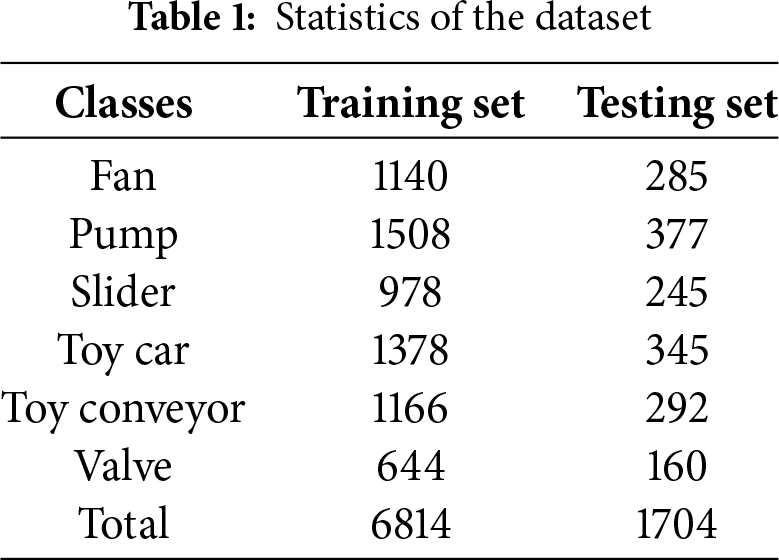
Figure 2: Spectrograms for the audio classification class

3.2 Deep Learning Models

For audio classification, DL models have proven to be immensely impactful, particularly in distinguishing between normal and anomalous audio samples. These models, which stand for neural network models and are often built using NN architectures, use sophisticated algorithms to automatically learn high-level representations of audio information so they can detect minute indicators of abnormalities or departures from the norm. In order to enable the network to abstract patterns and correlations, the model is trained on a varied data set that contains both regular and aberrant occurrences of audio samples. Once trained, the DL model’s remarkable ability to identify irregularities in real-time audio streams makes it invaluable for applications such as identifying faults in security systems, medical monitoring, and manufacturing equipment. The advantage of these models is that they can independently extract valuable information, offering a comprehensive and accurate classification technique in scenarios where differentiating between typical and unusual sounds is crucial.

CNNs are flexible models for distinguishing between normal and anomalous sound patterns. The ability of a CNN to automatically learn hierarchical feature representations through the use of convolutional filters is its greatest strength. These filters efficiently capture local patterns from audio, assisting the network in recognizing unique characteristics associated with both common and uncommon sounds. Convolutional layers often follow pooling layers in the architecture to downsample the dimension and extract important features.

LSTM networks, a type of softmaxed RNN aimed at detecting and sustaining long-term patterns in sequential data, make it simple to evaluate time-series data included in audio signals. The main advantage of LSTMs is their capacity to selectively retain or forget data over long stretches of time. This allows the model to recognize subtle temporal patterns in audio recordings. LSTM networks are said to be very efficient in the complex process of audio classification, especially in distinguishing between normal and unusual sound patterns.

The GRU model is a significant advancement, particularly suitable for audio classification. It can distinguish between normal and anomalous sound patterns. In order to improve the learning of long-term dependencies in sequential data, such as audio signals, GRUs are a form of RNN that was created to address some of the problems with vanishing gradients in conventional RNNs. The update gate (zt) and the reset gate (rt) are two gates in the GRU design that control data flow inside the network. The GRU model stands out as a robust and efficient tool for real-time audio classification tasks, demonstrating exceptional performance in discerning between normal and anomalous auditory events.

CRNN models have emerged as a powerful solution in the realm of audio classification, specifically in the discrimination between normal and anomalous sound patterns. CRNNs seamlessly merge the strengths of CNNs and RNNs, capitalizing on RNNs’ skill in simulating temporal relationships and CNNs’ capacity to capture spatial characteristics. The CRNN architecture is characterized by convolutional layers for feature extraction from spectrograms or other time-frequency representations, followed by recurrent layers for capturing sequential information.

The BiLSTM model has proven to be a good choice in the field of audio classification when it comes to distinguishing between normal and anomalous sound patterns. BiLSTMs build on the advantages of standard LSTMs by processing input sequences both forward and backward to capture interdependence in both past and future contexts. The LSTM formulation is mathematically generalized by the BiLSTM equations, which include both forward (ht) and backward (ht) hidden states.

Attention mechanisms models have revolutionized audio categorization, particularly in the ability to differentiate between typical and unusual sound patterns. By enabling the model to concentrate on particular input data items and give more weight to pertinent facts, attention mechanisms enhance neural network architectures. The model is able to dynamically pick various time-frequency components for audio thanks to attention techniques.

The capsule network, or CapsNet, is a novel approach to audio categorization and offers a fresh perspective on hierarchical feature learning. CapsNet is meant to overcome the limits of spatial hierarchies and posture variation, which sets it apart from traditional CNNs. CapsNets may be used to learn intricate patterns and relationships between sound sequences for audio categorization. The use of capsules, which are neuronal capsules that correlate to certain input properties, is innovative.

Residual networks (ResNet) have become a powerful architecture for audio classification tasks because of their ability to effectively learn deep feature representations without suffering from vanishing gradients. By introducing shortcut connections, ResNet allows information to bypass several layers, enabling the network to train deeper models while maintaining stability and accuracy. In audio classification, spectrograms (MFCCs) are often used as input, and ResNet efficiently extracts hierarchical patterns such as frequency variations and temporal dependencies. This makes it particularly suitable for recognizing complex sound events, environmental noises, or speech-related tasks where subtle differences in acoustic features play an important role. Overall, ResNet enhances generalization and robustness, offering improved performance compared to traditional convolutional networks in audio recognition problems.

EfficientNet is widely used in audio classification tasks because it balances accuracy and computational efficiency through compound scaling of network depth, width, and input resolution. Instead of arbitrarily increasing model size, EfficientNet systematically adjusts these dimensions, resulting in strong performance with fewer parameters and reduced training cost. When applied to audio data, features such as spectrograms are fed into the model, allowing it to capture both fine-grained frequency details and broader temporal patterns. This architecture is particularly effective in scenarios where large-scale audio datasets require high accuracy but also demand efficient resource utilization. Its ability to deliver strong generalization with lower computational overhead makes EfficientNet a reliable choice for sound recognition and classification tasks.

The HAM is a reliable technique used to improve model accuracy in audio classification problems. It works by helping the model concentrate on the key elements of the audio stream, including certain frequencies or intervals of time that hold important information. Instead of treating every area of the input equally, HAM gives different aspects different amounts of attention. This makes it possible for the model to identify patterns in the sound, especially in surroundings that are loud or ambiguous. HAM may enhance the performance of deep learning models in speech, music, and sound identification by combining several attention types, such as channel and spatial attention.

3.3 Proposed Ensemble Model

While originally devised for image recognition, the ensemble DL using LeNet and HAM models has found applicability in audio classification tasks, demonstrating its versatility beyond visual data analysis. The LeNet and HAM proposed architecture has proven effective in discerning between normal and anomalous sound patterns when adapted to audio processing. The core of the LeNet and HAM model involves pooling layers, convolutional layers, and fully connected layers. Although not originally designed for audio data, the LeNet and HAM architectures can be adapted to time-frequency representations of audio signals. Mathematically, the LeNet and HAM model is characterized by convolution (C), activation (A), and pooling (P) layers:

X0=XX1=ReLU(C65(X0))(Conv1)X2=P2(X1)(Avg/Max Pool1)X3=ReLU(C165(X2))(Conv2)X4=P2(X3)(Pool2)X5=HAM(X4)(Hybrid Attention Module)X6=Flatten(X5)X7=ReLU(D120(X6))X8=Dropout(X7,p=0.5)X9=Softmax(Dn(X8))(Output, n = number of classes)

where X is input tensor (image or 1D signal), C is convolutional layer with k filters and kernel size s, P is the pooling layer with pool size s, HAM(⋅) = Hybrid Attention Module, Dn = Dense (fully connected) layer with n neurons, ReLU = Rectified Linear Unit activation function, Softmax = Softmax activation function for output classification, Dropout = Dropout regularization layer.

Although not originally tailored for audio, the ensemble LeNet and HAM models showcase their adaptability, making them valuable tools in audio classification tasks, where discriminating between normal and anomalous sound patterns is paramount. LeNet was originally developed for image recognition tasks; however, spectrograms and MFCCs derived from audio can be naturally treated as two-dimensional time-frequency representations, similar to images. To adapt LeNet to this domain, we made the following modifications:

•   Input adaptation: MFCC features were structured as 2D arrays (time × frequency) and fed into the convolutional layers as image-like inputs.

•   Kernel and stride selection: Smaller convolutional kernels (e.g., 5 × 5) with a stride of 111 were used to capture fine-grained local spectral patterns over short time windows, as opposed to larger kernels often used in image processing.

•   Pooling operations: Max-pooling (2 × 2) with windows was applied to progressively reduce dimensionality while preserving dominant spectral features.

•   Regularization: Dropout layers were added after fully connected layers to prevent overfitting, given that audio datasets are often smaller than large-scale image datasets.

Table 2 provides the hyperparameters for each model. The architecture of the LeNet and HAM model is shown in Fig. 3. The module’s position is theoretically motivated based on feature abstraction levels:

•   Early layers: These capture low-level spectral features, which may include noise or irrelevant variations. Placing HAM here could overemphasize less informative details.

•   Middle layers: Feature maps at this stage contain sufficiently abstract and discriminative spectral-temporal patterns. HAM can effectively assign attention to the most relevant features, balancing local refinement and global context. This placement is theoretically optimal.

•   Late layers: Features are highly abstracted before classification. HAM here may have a limited impact since most salient features have already been aggregated.

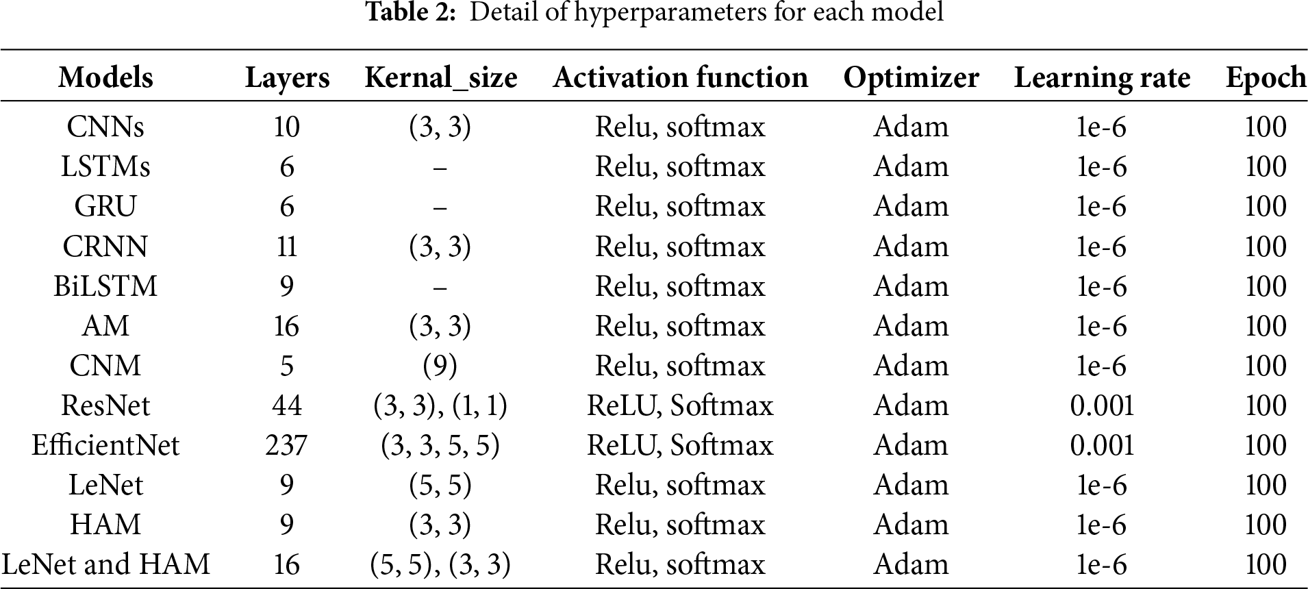
Figure 3: Proposed ensemble model architecture

According to attention theory, intermediate feature representations are most suitable for weighting because they retain meaningful patterns without being dominated by noise (early layers) or redundancy (late layers). Therefore, placing HAM in the middle layers is expected to maximize the model’s ability to detect vehicle mechanical defects from acoustic signals while improving generalization.

K-Fold Cross-Validation

In the ensemble LeNet and HAM architecture, employing the k-fold cross-validation proves pivotal for a robust appraisal of its effectiveness. Using this approach, the dataset is divided into k folds, or subsets of comparable size. The model undergoes k iterations during training, using a new fold as the validation set and the remaining folds for training each time. By using this method for overall evaluation, the likelihood of overfitting or underfitting is decreased. A more accurate evaluation of the model functionality is attained by averaging the performance metrics derived from each fold. The procedure highlights potential areas for improvement and offers valuable information on the model’s generalizability. Fig. 4 shows the ensemble model that has been proposed using LeNet and HAM with k-fold cross-validation.

Figure 4: Structure of the proposed approach using the k-fold cross-validation with the LeNet and HAM model

3.4 Evaluation Parameters

Several kinds of critical metrics are essential for evaluating the performance of audio categorization models. Precision, recall, and F1 score are the four basic measures that are frequently utilized.

A frequent performance statistic for evaluating the effectiveness of classification models, especially for multi-classification issues, is the Receiver Operating Characteristic-Area Under the Curve (ROC-AUC). With 1.0 being the ideal and 0.5 being no better than random guessing, a higher AUC is preferable.

ROC-AUC=∫01TPR(FPR)dFPR(1)

Whenever interacting with unbalanced datasets, classification models are assessed using the PR-AUC measure. A PR-AUC score close to 1.0 indicates that the model is performing exceptionally well in terms of accuracy and recall.

PR-AUC=∫01Precision(Recall)dRecall(2)

The standard deviation (σ) measures the variability of performance across folds:

σ=1n∑i=1n(xi−μ)2,μ=1n∑i=1nxi

The 95% confidence interval (CI) indicates the range in which the true mean lies with 95% certainty:

CI=μ±1.96×σn

4  Results and Discussion

The ability of DL models to accurately assess and comprehend data to make predictions is essential to their operation. Several metrics, including the accuracy, precision, recall, and F1 score, are used to evaluate deep learning models. The overall accuracy of a prediction determines its worth. The ratio of actual positive cases to all positive predictions is known as accuracy, whereas recall focuses on lowering false positives. All things considered, this offers a thorough understanding of the way a model performs across a range of data processing and prediction domains.

4.1 Performance of Convolutional Neural Networks

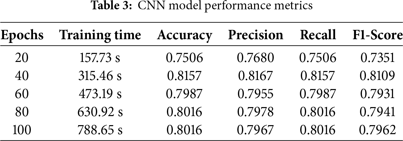
CNN’s performance in audio classification is excellent. They use evaluation measures including F1 score, accuracy, recall, and precision. Several experiments are conducted to evaluate CNN, and the DCASE 2020 datasets are used to identify patterns and trends. Precision computes the percentage of properly anticipated positive instances, whereas accuracy compares the proportion of correctly categorized cases to the overall sample size. Recall that 81.6% of the CNN algorithm was remarkable, with 81.57% accuracy, 81.67% precision, 81.09% F1 score, and a training duration of 788.65 s. These results show that the model can accurately predict outcomes and successfully capture positive cases, as shown in Table 3.

The predictions made by the CNN model utilizing testing data are shown in Fig. 5 as a confusion matrix. Results are displayed in a cross-section of actual and anticipated classifications, including “valve,” “fan,” “pump,” “slider,” “ToyCar,” and “ToyConveyor.” While the x-axis displays the expected outcomes, the y-axis displays the actual classes. The true prediction made by, for example, 0 classes in true classes and 380 valid predictions in predicted classes, is displayed on the confusion matrix’s diagonal. In the confusion matrix, every class displays the right guess in the same way. The CNN model shows a total of 1390 correct predictions out of 1654 total predictions, while 264 predictions are wrong.

Figure 5: Confusion matrix for CNN model

Fig. 6 shows the training accuracy and training loss graph. The model’s training is depicted in the training accuracy line graph, where the training line gradually changes during training to obtain an accuracy that is 80% higher than the training. The training results with validation accuracy above 80% are displayed by the orange line. The training loss that has been the lowest is displayed in the second graph. The CNN model training loss eventually dropped and produced results of less than 0.50%.

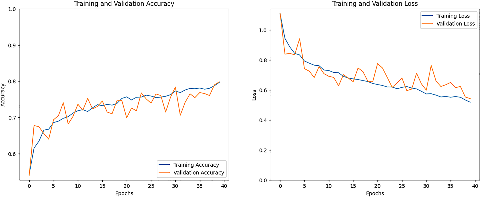
Figure 6: Accuracy and loss graph of the CNN model

4.2 Performance of Long Short-Term Memory

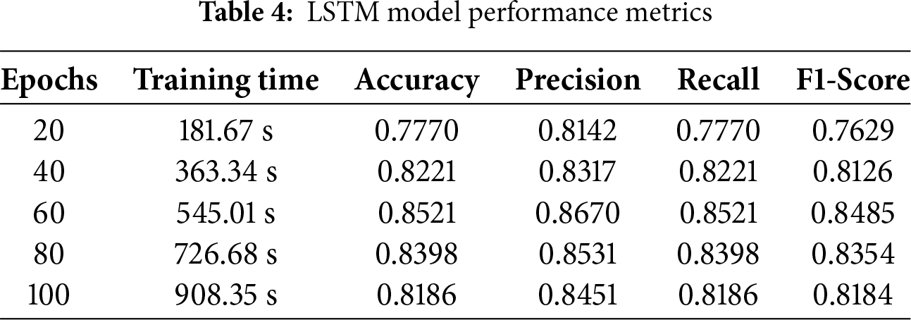
Whenever utilized for audio classification, LSTMs show remarkable efficacy using assessment metrics like accuracy, precision, etc. These networks are assessed using different test subsets from the DCASE 2020 datasets. The percentage of accurately anticipated positive instances is calculated by precision, whereas accuracy evaluates the proportion of properly categorized cases to the overall sample size. Optimizing weights and biases in LSTMs increases accuracy, precision, recall, and F1 scores. LSTMs are widely recognized for their efficiency and can be used to solve a range of categorization issues, particularly those using audio data. The impressive performance was demonstrated by the LSTM algorithm, with a recall of 85.21%, an accuracy of 85.21%, an F1-score of 84.85%, a precision of 86.7%, and a 545.01-s training period. These results show that the model can precisely forecast occurrences and successfully identify positive cases, as shown in Table 4.

The LSTM model using the testing data made predictions for testing samples, which are shown in Fig. 7 as a confusion matrix. Results are presented in a cross-section of actual and anticipated classifications, including “valve,” “fan,” “pump,” “slider,” “ToyCar,” and “ToyConveyor.” The true prediction made by, for example, 0 classes in true classes and 430 valid predictions in predicted classes, is displayed on the confusion matrix’s diagonal. In the confusion matrix, every class illustrates the right guess in the same way. Total correct predictions are 1452, while 202 predictions are wrong.

Figure 7: Confusion matrix for LSTM model

The training accuracy and training loss graph will be seen in Fig. 8. The model’s training is depicted on the training accuracy line graph, where the training line gradually changes during training to achieve an accuracy that is 85% higher than training. The training results with validation accuracy above 85% are displayed by the orange line. The training loss that has been the lowest will appear in the second graph. The CNN model training loss steadily dropped and produced results that were less than 0.40%.

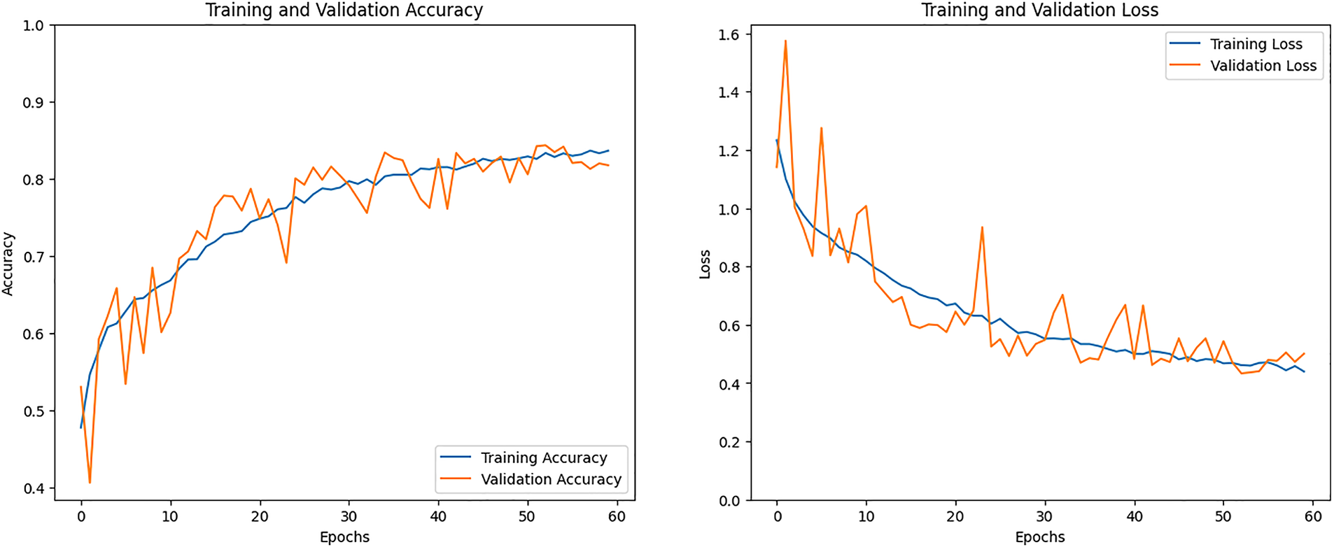
Figure 8: Accuracy and loss graph of the LSTM model

4.3 Performance for Gated Recurrent Unit

GRU illustrated the incredible effectiveness of managing audio classification obligations by utilizing evaluation criteria such as F1 score, recall, accuracy, and precision. The models are assessed using different test datasets and provide insights into patterns and characteristics from the DCASE 2020 datasets. In opposition to accuracy, it determines the proportion of correctly predicted positive cases; accuracy contrasts the number of correctly classified cases with the total sample size.

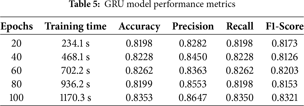
The GRU’s recall, accuracy, precision, and F1 score were all impressive, ending the training phase with 83.5%, 83.53%, 86.47%, 83.21%, and 1170.3 s, respectively. The results show that the capability of GRU used to make accurate predictions and successfully capture positive cases, as shown in Table 5.

Each of the sets of predictions made by the GRU model utilizing testing data is shown in Fig. 9 as a confusion matrix. Results are displayed in a cross-section of actual and anticipated classifications, including “valve,” “fan,” “pump,” “slider,” “ToyCar,” and “ToyConveyor.” The true prediction made by, for example, 0 classes in true classes and 439 valid predictions in predicted classes, is displayed on the confusion matrix’s diagonal. In the confusion matrix, every class exhibits the right guess in the same way. The GRU model predicts 1423 predictions correctly, while 231 predictions are wrong.

Figure 9: Confusion matrix for GRU model

The training accuracy and training loss graph are presented in Fig. 10. The model’s training is depicted on the training accuracy line graph, where the training line gradually changes during training to obtain an accuracy that is 80% higher than training. The training results with validation accuracy above 80% are represented by the orange line. The training loss that has been the lowest can be observed in the second graph. With time, the CNN model training loss was reduced and produced results that were less than 0.40%.

Figure 10: Accuracy and loss graph of the GRU model

4.4 Performance of Convolutional Recurrent Neural Network

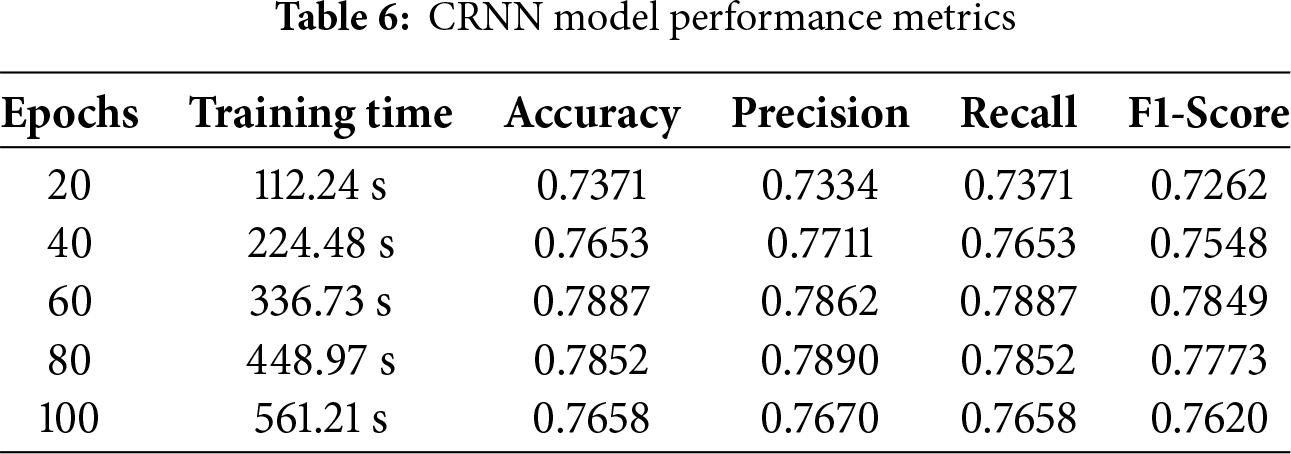
Although implemented in audio classification tasks, CRNN demonstrated remarkable efficacy using assessment criteria including precision, accuracy, recall, and F1 score. Several test datasets from the DCASE 2020 dataset are used to evaluate CRNN. Precision indicates the percentage of accurately projected positive instances, and accuracy quantifies the proportion of correctly organized cases to the general sample size. By maximizing their weights and biases, CRNNs improve accuracy, precision, recall, and F1 scores. CRNNs are widely recognized for their efficiency and can be used for a number of categorization tasks, particularly those using audio data. Impressive results were obtained by the CRNN algorithm: recall of 78.87%, accuracy of 78.87%, precision of 78.62%, F1-score of 78.49%, and 336.78 s to end the training session. As seen in Table 6, these findings illustrate the model’s ability to correctly collect positive instances and forecast outcomes.

Using testing data in the confusion matrix layout, Fig. 11 depicts the full predictions of the CRNN model. Results are displayed in a cross-section of actual and anticipated classifications, including “valve,” “fan,” “pump,” “slider,” “ToyCar,” and “ToyConveyor.” The CRNN model predicts 1344 correct predictions, while 360 predictions are wrong.

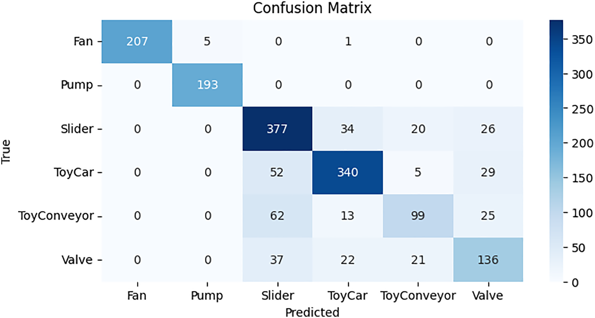
Figure 11: Confusion matrix for CRNN model

The training accuracy and training loss graph are displayed in Fig. 12. The model’s training performance is shown on the training accuracy line graph, where the training line gradually changes during training to obtain an accuracy that is 80% higher than the training. The training results with validation accuracy above 80% are displayed by the orange line. The training loss that has been the lowest is displayed in the second graph. The CNN model training loss steadily dropped and produced results that were less than 0.50%.

Figure 12: Accuracy and loss graph of the CRNN model

4.5 Performance of Bidirectional Long Short-Term Memory Networks

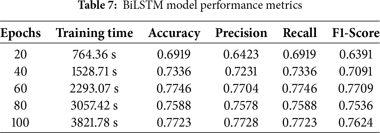
While employed for audio classification problems, BiLSTM reveals remarkable efficacy using assessment measures including accuracy, precision, recall, and F1 score. The model is assessed using the DCASE 2020 dataset. Precision obtains the percentage of properly anticipated positive instances, whereas accuracy compares the proportion of accurately designated cases to the overall sample size. BiLSTM improves accuracy, precision, recall, and F1 scores by optimizing weights and biases. The impressive performance was demonstrated by the BiLSTM algorithm, with a recall of 75.88%, an accuracy of 75.88%, an F1-score of 75.36%, a precision of 75.78%, and 2293.07 s to end the training time. The results obtained indicate the model can accurately predict situations and successfully capture positive cases, as shown in Table 7.

The predictions made by the BiLSTM model utilizing testing data are shown in Fig. 13 as a confusion matrix. Results are displayed in a cross-section of actual and anticipated classifications, including “valve,” “fan,” “pump,” “slider,” “ToyCar,” and “ToyConveyor.” The BiLSTM model shows poor performance compared to CNN, GRU, and CRNN models, with only 1293 correct predictions, fewer than the other models, while 361 predictions are predicted incorrectly.

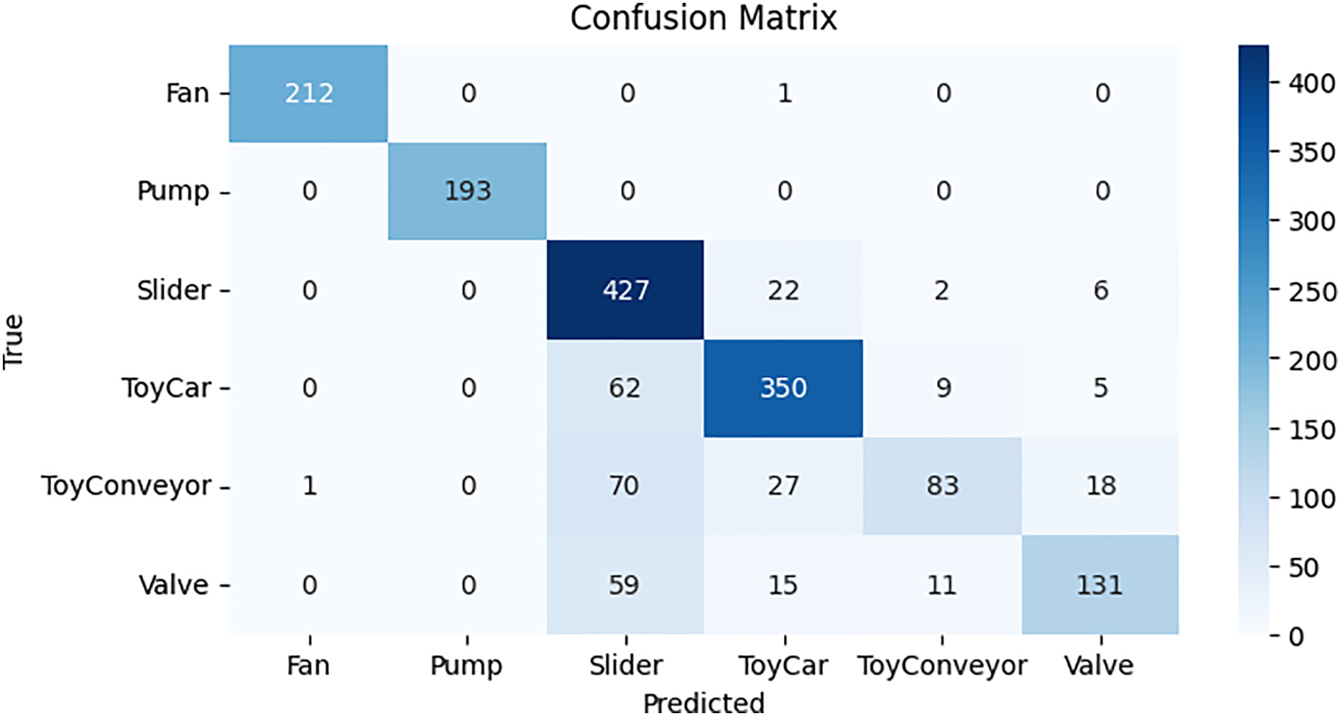
Figure 13: Confusion matrix for BiLSTM model

The training accuracy and training loss graph will be seen in Fig. 14. The model’s training is depicted in the training accuracy line graph, where the training line gradually changes during training to achieve a 75% increase in training accuracy. The validation accuracy in training outcomes above 75% is displayed by the orange line. The training loss that has been the lowest is displayed in the second graph. Less than 0.60 percent of the CNN model training loss was attained over time.

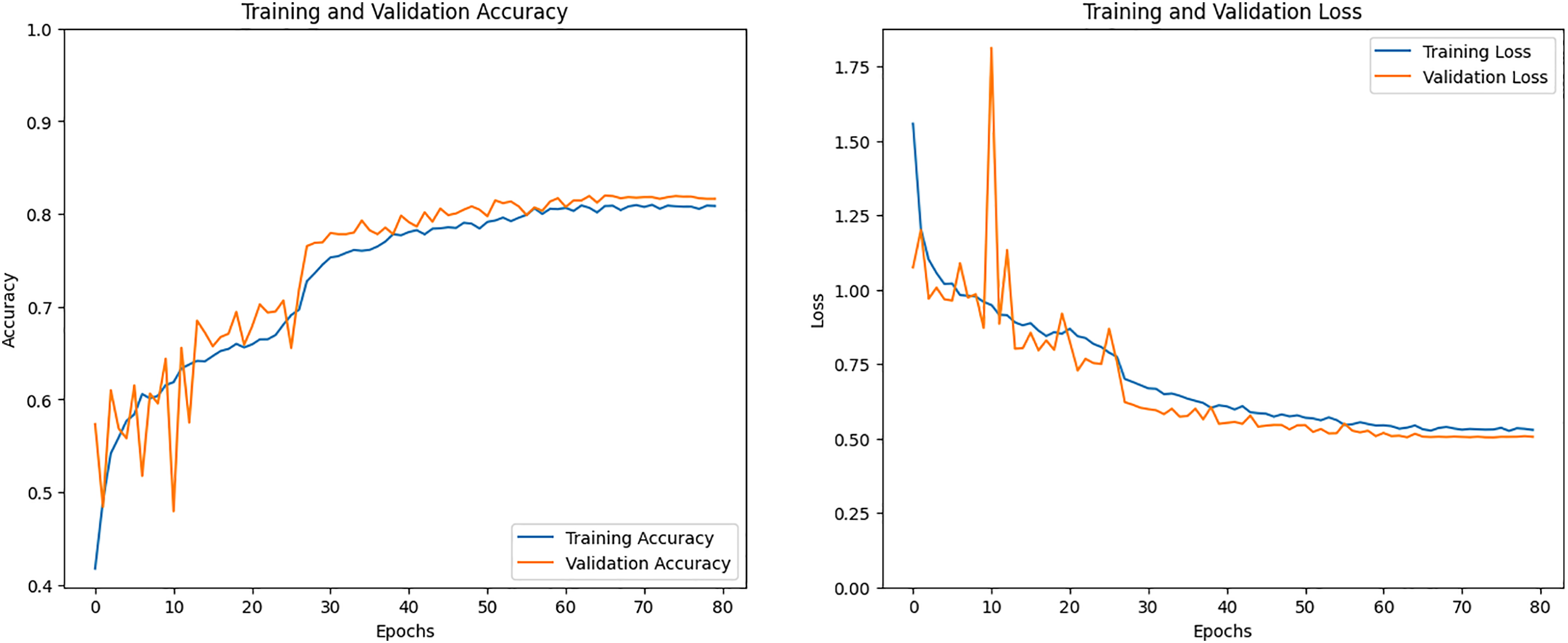
Figure 14: Accuracy and loss graph of the BiLSTM model

4.6 Performance of Attention Mechanism

In regard to audio categorization tasks, AM provides exceptional efficacy concerning recall, F1 score, etc. These networks are assessed using different test datasets and gain insights into patterns and characteristics from the DCASE 2020 datasets. Precision reflects the percentage of accurately projected positive instances, and accuracy indicates the proportion of correctly classified cases to the general sample size. By maximizing their weights and biases, AM improves accuracy, precision, recall, and F1 scores. The impressive performance was demonstrated by the AM algorithm, with a recall of 83.27%, accuracy of 83.27%, an F1 score of 82.39%, a precision of 84.77%, and 1933.38 s per training period. The results presented here show that the model can accurately predict occurrences and successfully capture positive cases, as shown in Table 8.

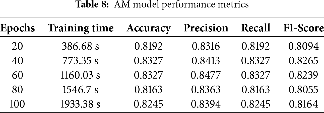
Fig. 15 shows the confusion matrix for all classes using the AM model on test data. Results are displayed in a cross-section of actual and anticipated classifications, including “valve,” “fan,” “pump,” “slider,” “ToyCar,” and “ToyConveyor.” The confusion matrix reveals that the AM model shows superior performance compared to CNN, gRU, CRNN, and BiLSTM, with 1391 correct predictions. On the other hand, 263 predictions are wrong.

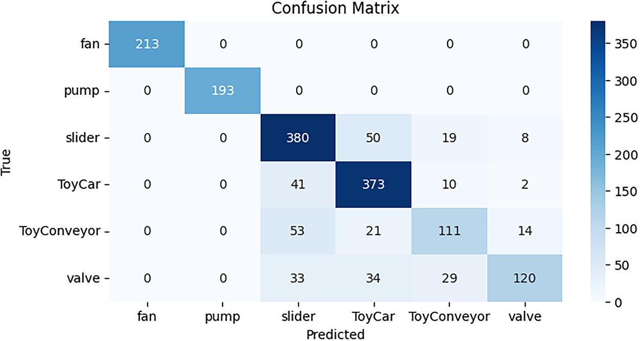
Figure 15: Confusion matrix for AM model

The training accuracy and training loss graph are presented in Fig. 16. The model’s training is depicted on the training accuracy line graph, where the training line gradually changes during training to obtain an accuracy that is higher than 80%. The training results with validation accuracy above 80% are displayed by the orange line. The training loss that has been the lowest is displayed in the second graph. Less than 0.60 percent of the CNN model training loss was attained over time.

Figure 16: Accuracy and loss graph of the AM model

4.7 Performance for Capsule Network Model

The moment it relates to audio classification tasks, CNM conveys extraordinary effectiveness by utilizing several assessment criteria. These networks are assessed using different test datasets and gain insights into patterns and characteristics from the DCASE 2020 datasets. Precision estimates the percentage of properly anticipated positive instances, whereas accuracy compares the proportion of correctly designated cases to the broad sample size. Impressive performance was demonstrated by the CNM model, with recall, accuracy, precision, and F1 score of 77.64%, 77.64%, and 76.76%, and a 718.13-s training period, respectively. These results display that the model can accurately predict consequences and successfully capture positive cases, as shown in Table 9.

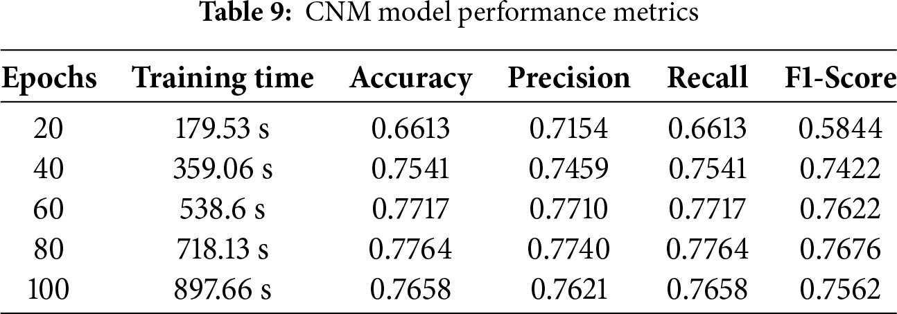
Fig. 17 shows the confusion matrix of the CNM model, showing its performance on the test samples. As evident from Fig. 17, the models predict 1323 samples correctly, comprising true positives and true negatives, while 331 predictions are wrong.

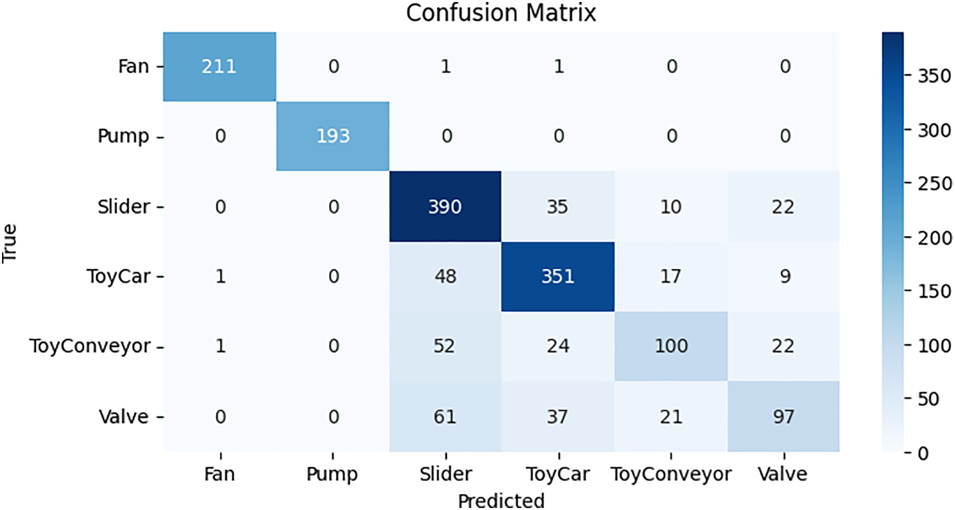
Figure 17: Confusion matrix for CNM model

The training accuracy and training loss graph can be seen in Fig. 18. The model’s training is depicted on the training accuracy line graph, where the training line gradually changes during training to obtain an accuracy that is 80% higher than the training. The training results with validation accuracy above 80% are displayed by the orange line. The training loss that has been the lowest can be seen in the second graph. Less than 0.60 percent of the CNN model training loss was attained over time.

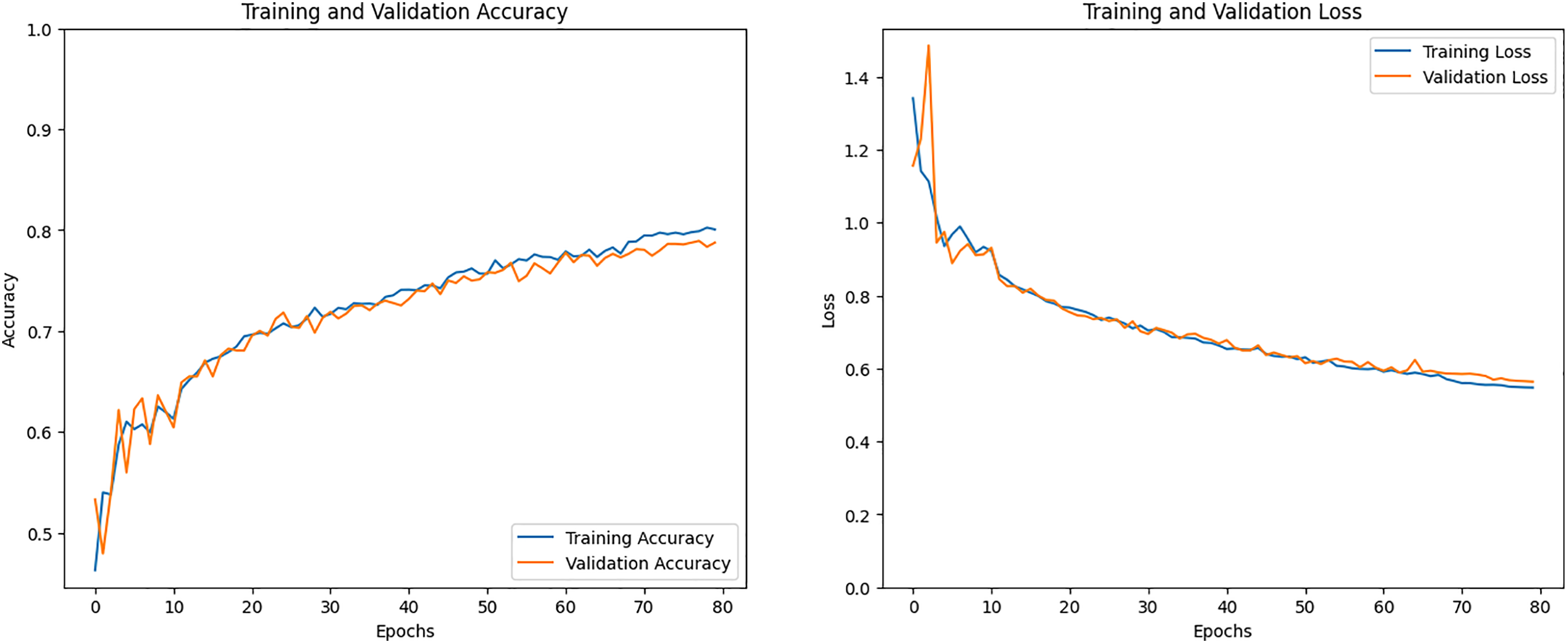
Figure 18: Accuracy and loss graph of the CNM model

4.8 Performance for ResNet Model

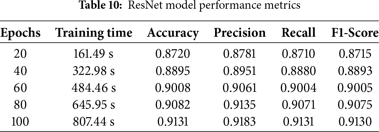
ResNet has exceptional efficacy when applied to audio classification problems by employing many evaluation criteria. Several test datasets are used to evaluate these networks, and the DCASE 2020 datasets provide information on trends and traits. While accuracy compares the proportion of correctly classified cases to the whole sample size, precision calculates the percentage of correctly expected positive instances. With an 807.44-s training period and recall, accuracy, precision, and F1 score of 91.31%, 91.31%, 91.83%, and 91.30%, respectively, the ResNet algorithm showed impressive performance. These findings demonstrate that the model can successfully collect positive instances and forecast outcomes with accuracy, shown in Table 10.

The confusion matrix of the ResNet model, demonstrating its performance on the test samples, is displayed in Fig. 19. The models properly predict 1556 samples, including true positives and true negatives, as shown in Fig. 19, whereas 146 predictions are incorrect.

Figure 19: Confusion matrix for ResNet model

Fig. 20 displays the training accuracy and training loss graph. The training accuracy line graph shows the model’s training, with the training line progressively changing during training to achieve an accuracy that is 90% greater than the training. The orange line shows training outcomes with validation accuracy more than 80%. The second graph shows the training loss that has been the lowest. Over time, the CNN model training loss was less than 0.60.

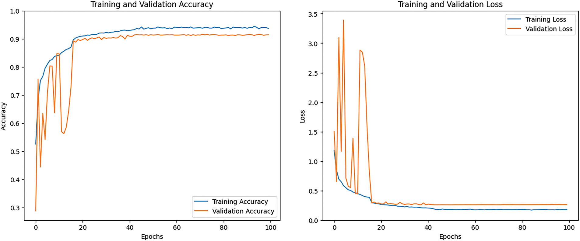
Figure 20: Accuracy and loss graph of the ResNet model

4.9 Performance for EfficientNet Model

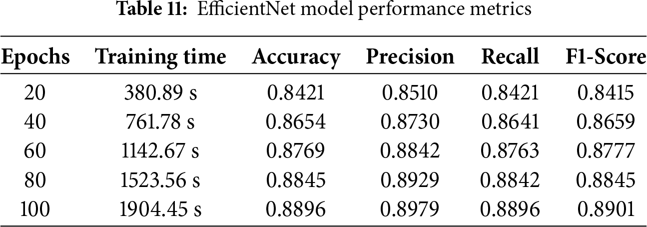
EfficientNet uses various kinds of evaluation criteria to demonstrate exceptional efficacy when it comes to audio categorization tasks. Several test datasets are used to evaluate these networks, and the DCASE 2020 datasets provide information on trends and traits. While accuracy compares the proportion of correctly classified cases to the whole sample size, precision calculates the percentage of correctly expected positive instances. With a 1904.45-s training period and recall, accuracy, precision, and F1-score of 88.96%, 88.96%, 89.79%, and 89.01%, respectively, the EfficientNet method showed impressive performance. These findings demonstrate that the model can collect positive instances and forecast outcomes with accuracy, as seen in Table 11.

The confusion matrix of the EfficientNet model, demonstrating its effectiveness on the test samples, is displayed in Fig. 21. The models properly forecast 1516 samples, including true positives and true negatives, as shown in Fig. 21, while making 193 incorrect predictions.

Figure 21: Confusion matrix for EfficientNet mode

Fig. 22 displays the training accuracy and training loss graph. The training accuracy line graph shows the model’s training, with the training line progressively changing during training to achieve an accuracy that is 90% greater than the training. The orange line shows training outcomes with validation accuracy more than 90%. The second graph shows the training loss that has been the lowest. Over time, the CNN model training loss was less than 0.25.

Figure 22: Accuracy and loss graph of the EfficientNet model

4.10 Performance of LeNet Model

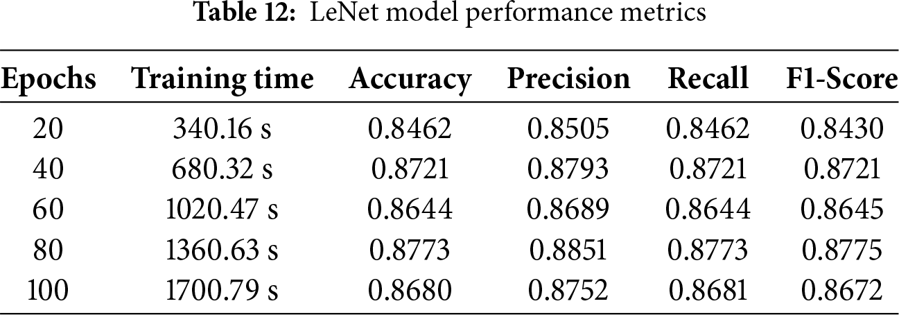
LeNet exhibits outstanding effectiveness in handling audio classification problems by using evaluation standards, such as accuracy, precision, recall, and F1 score. These networks are assessed using different test datasets and gain insights into patterns and characteristics from the DCASE 2020 datasets. Precision reflects the percentage of accurately projected positive instances, and accuracy quantifies the proportion of correctly organized cases to the general sample size. With a recall of 87.73%, accuracy of 87.73%, precision of 88.51%, F1-score of 87.75%, and 1360.63 s on the way to finishing the training, the LeNet algorithm performed admirably. Table 12 illustrates these results, which suggest that the model can successfully capture positive instances and forecast effects with accuracy.

The LeNet model’s predictions for each class are displayed as a confusion matrix and are shown in Fig. 23. Results are displayed in a cross-section of actual and anticipated classifications, including “valve,” “fan,” “pump,” “slider,” “ToyCar,” and “ToyConveyor.” The LeNet model remarkably predicts 1495 correctly, with only 159 wrong predictions, which is the least number compared to all other models.

Figure 23: Confusion matrix for LeNet model

Fig. 24 illustrates the training accuracy and training loss graph. The model’s training is depicted in the training accuracy line graph, where the training line gradually changes throughout training and reaches 90% above training accuracy. The validation accuracy in training reached above 90% outcomes, as shown by the orange line. The training loss that has been the lowest is displayed in the second graph. The LeNet model training loss steadily dropped and produced results that were less than 0.20.

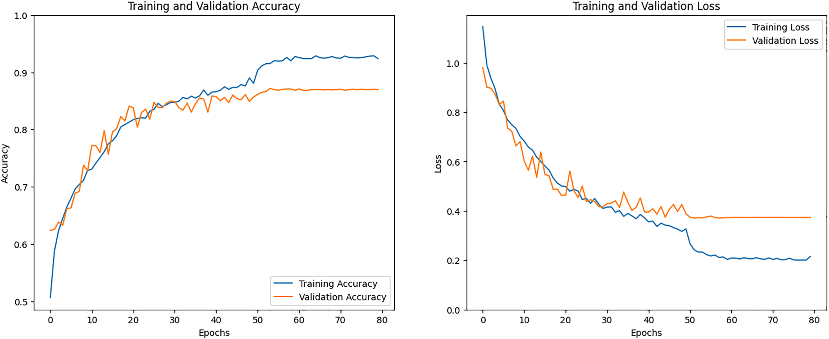
Figure 24: Accuracy and loss graph of the LeNet model

4.11 Performance of Hierarchical Attention Mechanism (HAM) Model

The HAM model shows strong performance in audio classification tasks by using evaluation metrics such as recall and accuracy. F1 score and precision. It is tested on various datasets, including the DCASE 2020 dataset, to understand different patterns and features. Precision measures how many of the predicted positive cases are correct, while accuracy shows the percentage of total correct predictions. The HAM model achieved an accuracy of 84.53%, a precision of 84.99%, a recall of 84.53%, an F1 score of 84.57%, and 432.52 s brought the training session to a finish. Table 13 presents these results, indicating that the model is effective in identifying correct instances and making accurate predictions.

The HAM model’s predictions for each class are shown in the confusion matrix in Fig. 25. The results include actual and predicted labels for classes such as “valve,” “fan,” “pump,” “slider,” “ToyCar,” and “ToyConveyor.” The HAM model correctly predicted 1485 samples and made only 251 incorrect predictions, which is fewer than any other model tested.

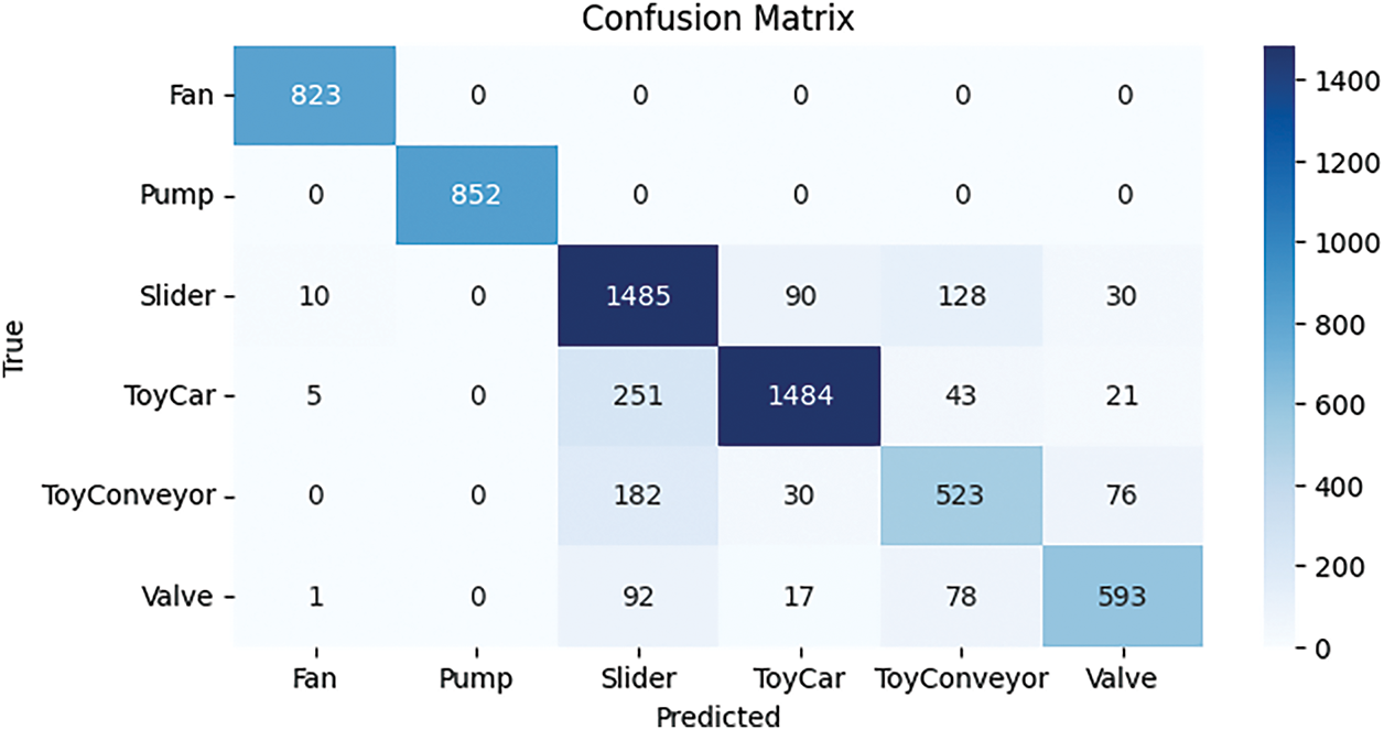
Figure 25: Confusion matrix for HAM model

Fig. 26 shows the graphs for training accuracy and training loss. The first graph displays the training accuracy, where the model’s accuracy steadily improves during training and reaches above 80%. The orange line in the graph shows the validation accuracy, which also goes above 80%. The second graph shows the training loss, which keeps decreasing as the model learns. The HAM model’s training loss dropped consistently and reached below 0.40%, showing that the model was learning well over time.

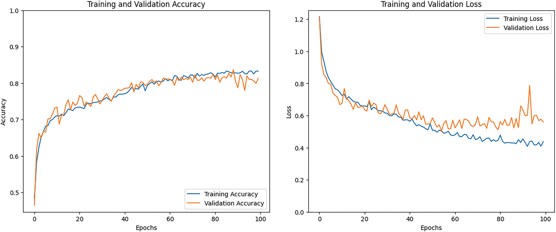
Figure 26: Accuracy and loss graph of the Hierarchical Attention Mechanism (HAM) model

4.12 Performance of Proposed Ensemble Model

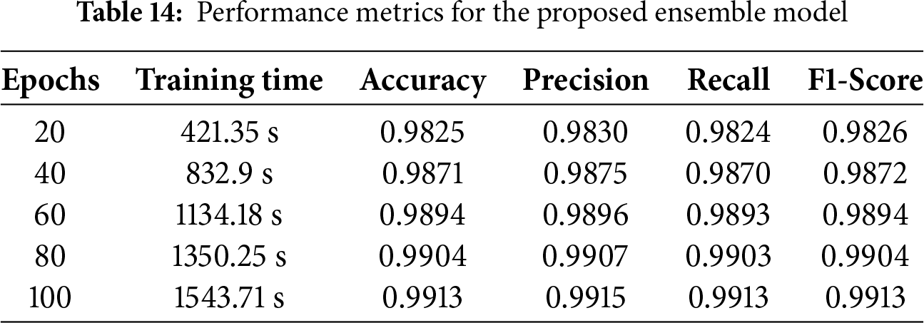
The proposed ensemble model using LeNet and HAM models shows strong performance in solving audio classification tasks by using key evaluation metrics such as accuracy, precision, recall, and F1 score. These models are tested on various datasets, including the DCASE 2020 dataset, to better understand sound patterns and features. The LeNet and HAM model reached the highest 99.13% in accuracy and 99.13% in recall, 99.15% in precision, 99.13% in F1 score, and 1543.71 s for the period of the training session. Similarly, the HAM model also produced strong results, confirming their effectiveness in correctly identifying and predicting audio events. Table 14 presents these outcomes, highlighting the models’ reliable performance.

The predictions made by the LeNet and HAM model for each class are shown in the confusion matrix in Fig. 27. The results compare the actual and predicted labels for different classes, including “valve,” “fan,” “pump,” “slider,” “ToyCar,” and “ToyConveyor.” The LeNet and HAM model correctly predicted 1797 samples and made only 27 incorrect predictions. This is the lowest number of errors compared to all other models, showing its high accuracy and reliable performance.

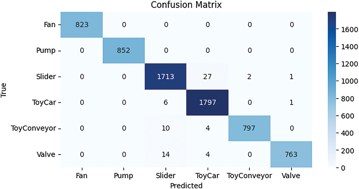
Figure 27: Confusion matrix for the LeNet and HAM model

Fig. 28 shows the training accuracy and training loss graphs for the ensemble LeNet and HAM model. In the first graph, the training accuracy increases gradually during the training process and goes above 80%. The orange line represents the validation accuracy, which also rises above 80%, showing good performance on unseen data. The second graph displays the training loss, which continues to decrease as the model learns. The LeNet and HAM model’s training loss dropped steadily and went below 0.45%, indicating effective learning and better results over time.

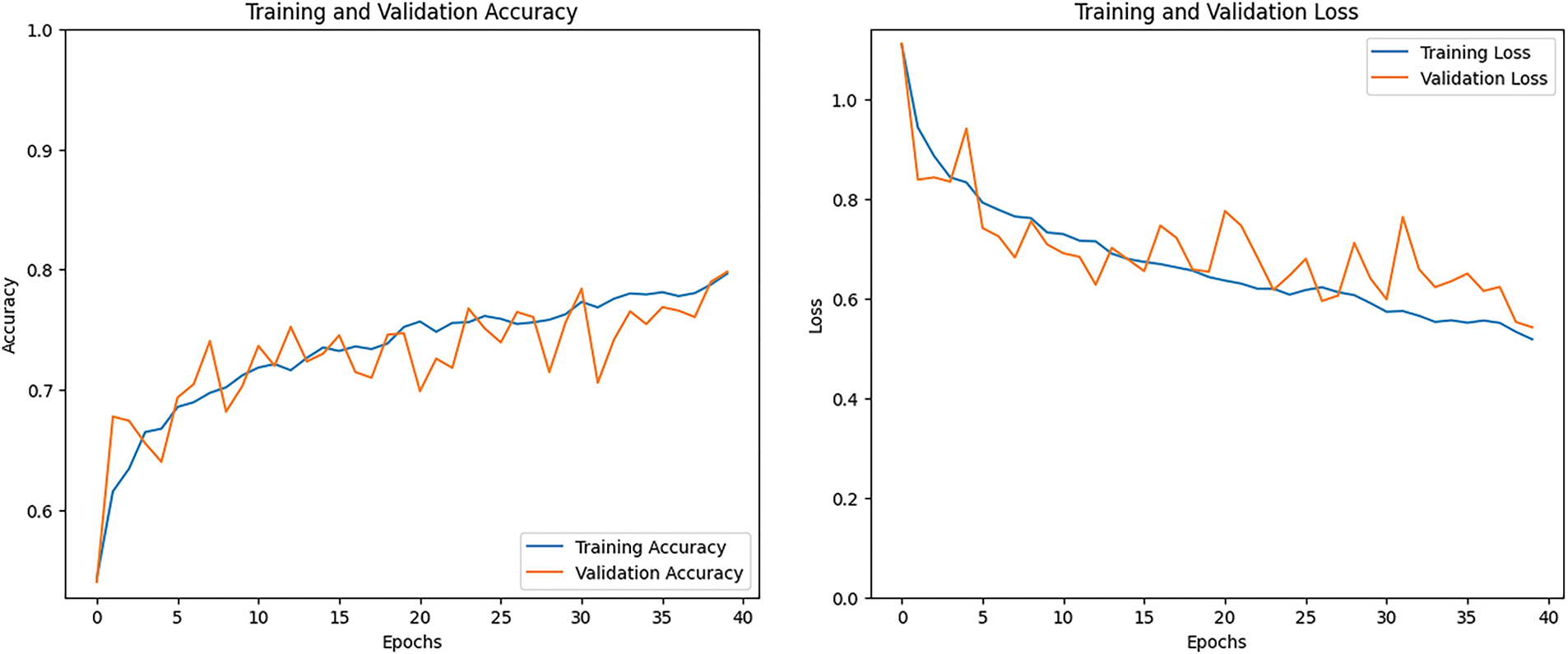
Figure 28: Accuracy and loss graph of the LeNet and HAM model

4.13 Performance Comparison across All K-Fold Cross-Validation

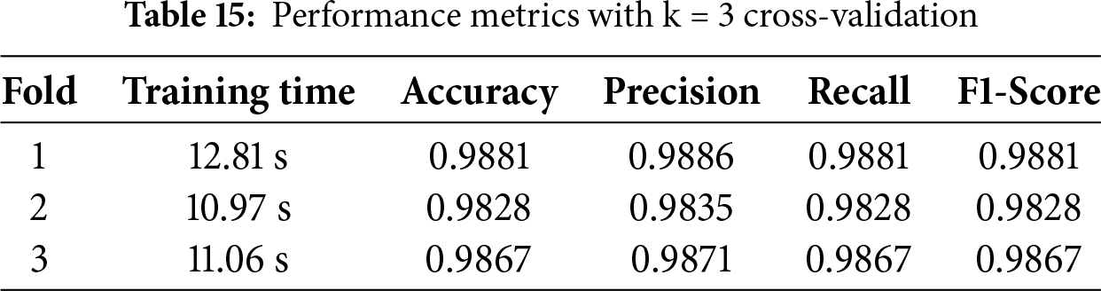
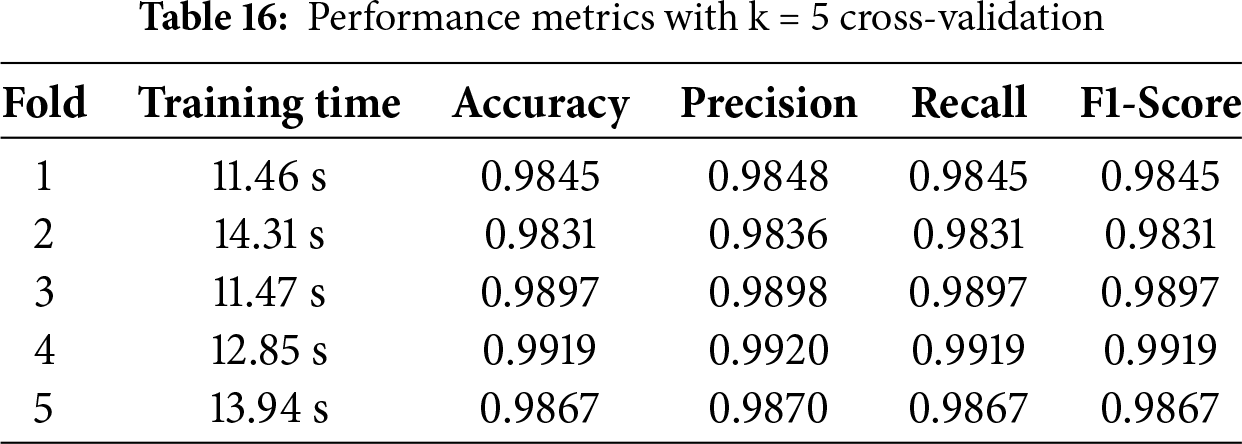
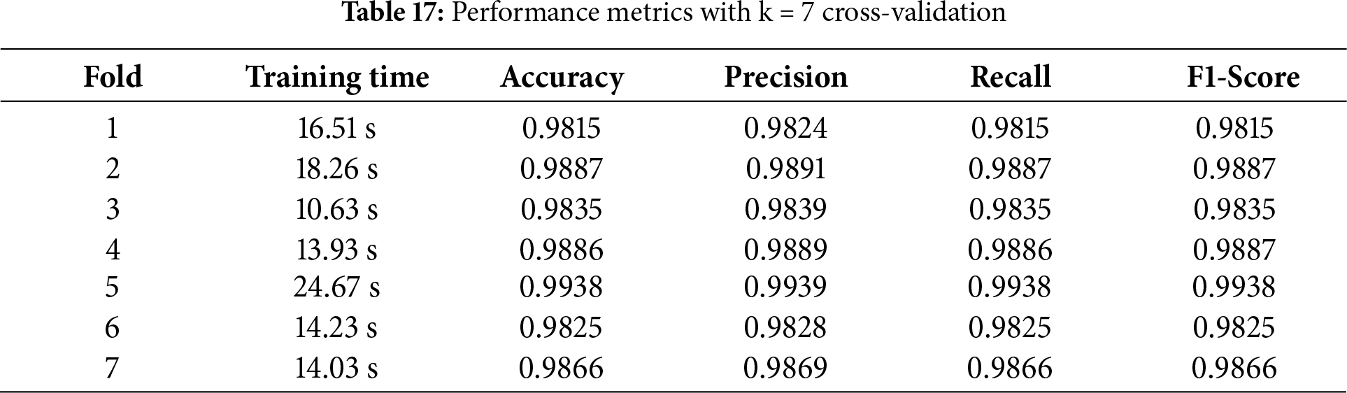
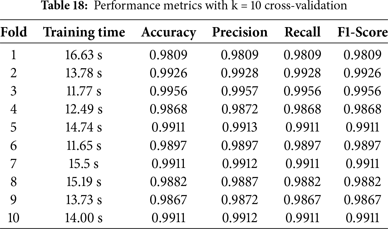
For the validation of the model’s performance, k-fold cross-validation is required for the proposed approach. Tables 15–18 display the results for k = 3, 5, 7, and 10 in that order. The outcome shows that Table 18, where k = 10, performs much better than other tables.

K-fold cross-validation shows a slightly better performance of the models than what is reported for the test set. This outcome can be explained by the following factors:

i.   More stable training-validation split: The non-K-fold model relies on a single 80/20 train-test split, which may introduce sampling bias depending on how the data is partitioned. K-fold cross-validation mitigates this by averaging results over multiple folds, ensuring that all samples participate in both training and validation, thereby reducing variance.

ii.   Regularization effect: Since the model is retrained multiple times across different subsets, the ensemble-like effect of K-fold evaluation provides more reliable generalization. This process can yield slightly higher average accuracy compared to a single run, especially in moderately sized datasets such as ours.

iii.   Balanced utilization of minority patterns: For imbalanced datasets, some rare patterns may not appear in the training set during a single split. K-fold ensures these minority patterns are included in training at least once, leading to improved recall and F1 score across folds.

Therefore, the observed improvement of models using cross-validation is not anomalous but rather a reflection of the more comprehensive training validation scheme inherent to K-fold evaluation.

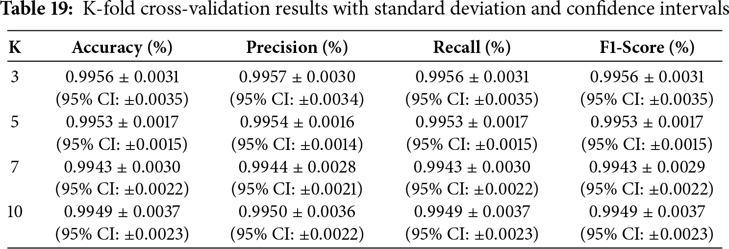
4.14 Performance of Standard Deviation (SD) and Confidence Intervals (CI)

In calculating the proposed model stability and generalizability, we examined cross-validation performance based on standard deviation and confidence intervals over different folds. By including these statistical metrics, the stability of the model performance may be better understood than with only mean values. More confidence in the predicted performance values is shown by shorter confidence intervals, while a reduced standard deviation indicates that the model performance is constant across different data splits. The findings show that the model consistently achieved 99.4% across all metrics, indicating excellent classification capability. The standard deviation (ranging from ±0.0016 to ±0.0037) and narrow confidence intervals highlight the model stability and reliability across different folds. The model shows the least fluctuation in accuracy, precision, recall, and F1-score, as shown in Table 19. This indicates that it is less likely to overfit and has satisfactory generalization. These outcomes attest to the model’s resilience and dependability.

4.15 ROC-AUC and PR-AUC Performance Metrics

To achieve better classification results, this study investigated different types of DL models such as CNN, LSTM, BLSTM, GRU, CRNN, AM, CNM, ResNet, EfficientNet, LeNet, HAM, and LeNet and HAM. The performance of these models is evaluated using ROC-AUC and PR-AUC metrics. These metrics help measure how well the models classify data and provide a clear understanding of their classification capabilities. Figs. 29 and 30 show the results for PR-AUC and ROC-AUC. The results in Table 20 also include a comparison of the macro-average values for all models.

Figure 29: Performance regarding ROC-AUC curve

Figure 30: Performance regarding PR-AUC curve

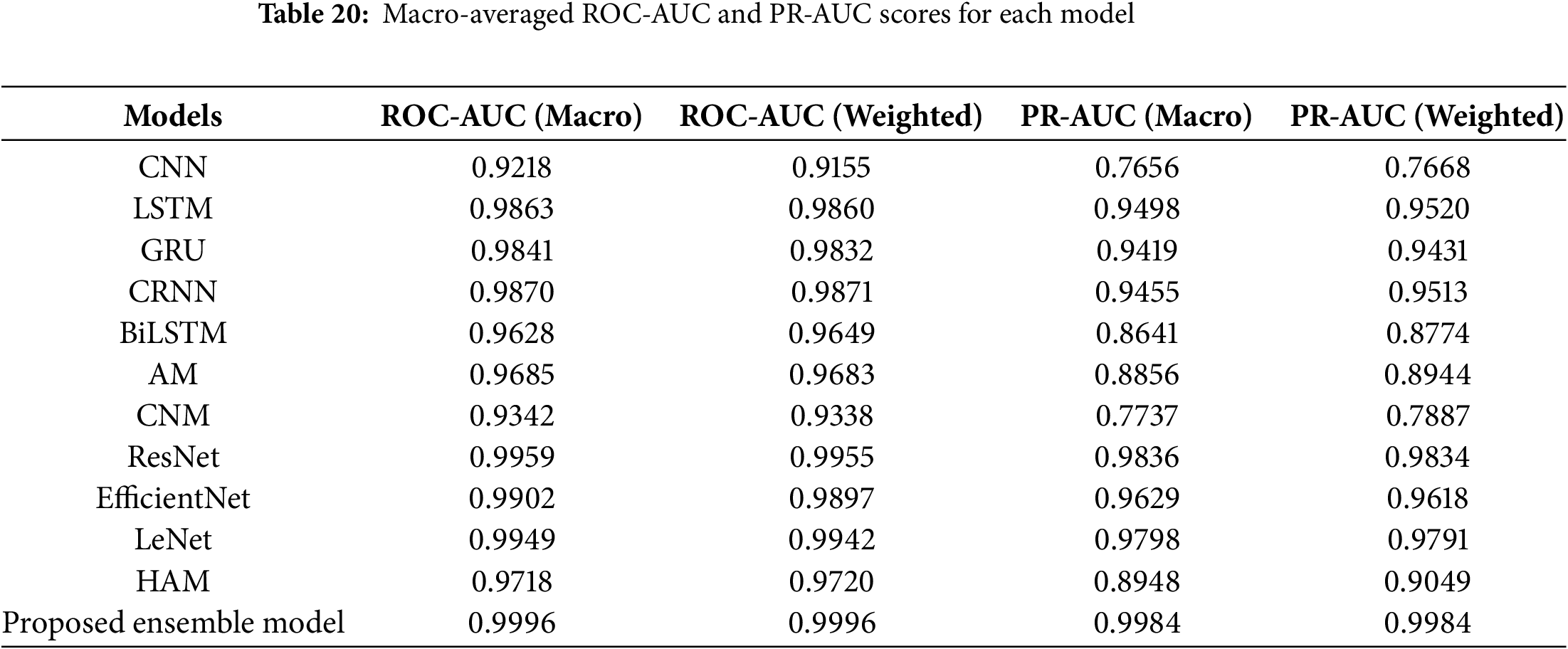
Results in Table 20 indicate that the performance of various models varies significantly. Regarding the performance differences, it is attributed to the distinctive modeling capacities of the architectures. CNN-based models (CNN, LeNet) efficiently capture spectral patterns but may struggle with long-term dependencies, whereas recurrent models (ResNet, EfficientNet, BiLSTM) perform better at temporal modeling but incur higher computational cost and sometimes lower generalization when the dataset is limited. CRNN achieves a balance by combining both aspects. Attention mechanisms improve feature weighting, while capsule networks are more experimental and showed moderate performance in our setting. The superior performance of the proposed ensemble model reflects its ability to integrate complementary strengths of these architectures, resulting in improved generalization across test data.

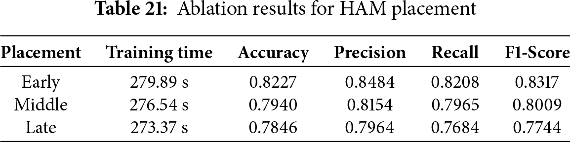
4.16 Ablation Study on Attention Placement

The HAM placement within the network, an ablation study was conducted with three configurations: early, middle, and late insertion. The results in Table 21 indicate that positioning the module in the middle layers provides the best balance across accuracy, precision, recall, and F1 score. When located in the early layers, the attention mechanism emphasizes low-level patterns such as edges or raw frequency bands, but this narrow focus on shallow details restricts the extraction of higher-level semantic features, resulting in weaker performance. Placement in the final layers offers some improvement, yet at this stage, the representations are already highly compressed, which limits the capacity of attention to refine feature learning. The superior outcomes achieved through middle-layer placement suggest that attention functions most effectively after local features have been established but before the information is fully condensed, enabling integration of both detailed and global context. These findings reinforce the architectural choice and correspond with theoretical insights reported in prior studies on attention mechanisms.

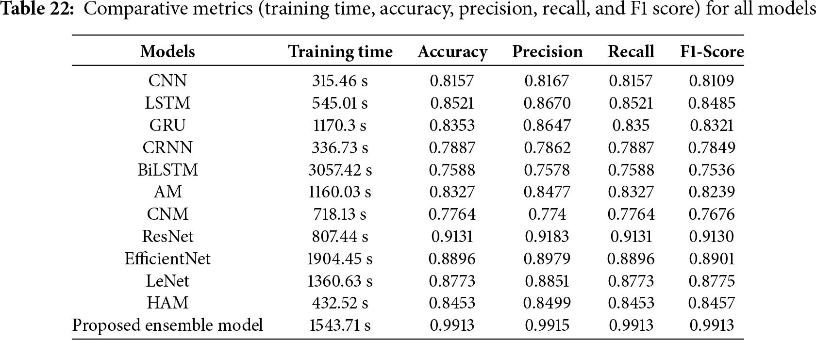
4.17 Comparative Analysis of All Models with DCASE 2020 Dataset

The findings of every model used in the present study are shown in Table 22. The suggested model outperforms the other models, CNN, LSTM, GRU, CRNN, BiLSTM, AM, CNM, ResNet, EfficientNet, LeNet, and HAM model, all of which have been optimized to produce the best results with the given dataset. Nevertheless, the proposed model performs better than any other model now in use. In DL, hyperparameters are either user-supplied or selected via hyperparameter optimization methods. These parameters define the structure and capabilities of a deep learning model. Whereas the model parameters, which are learned during the training phase, hyperparameters affect the learning process itself.

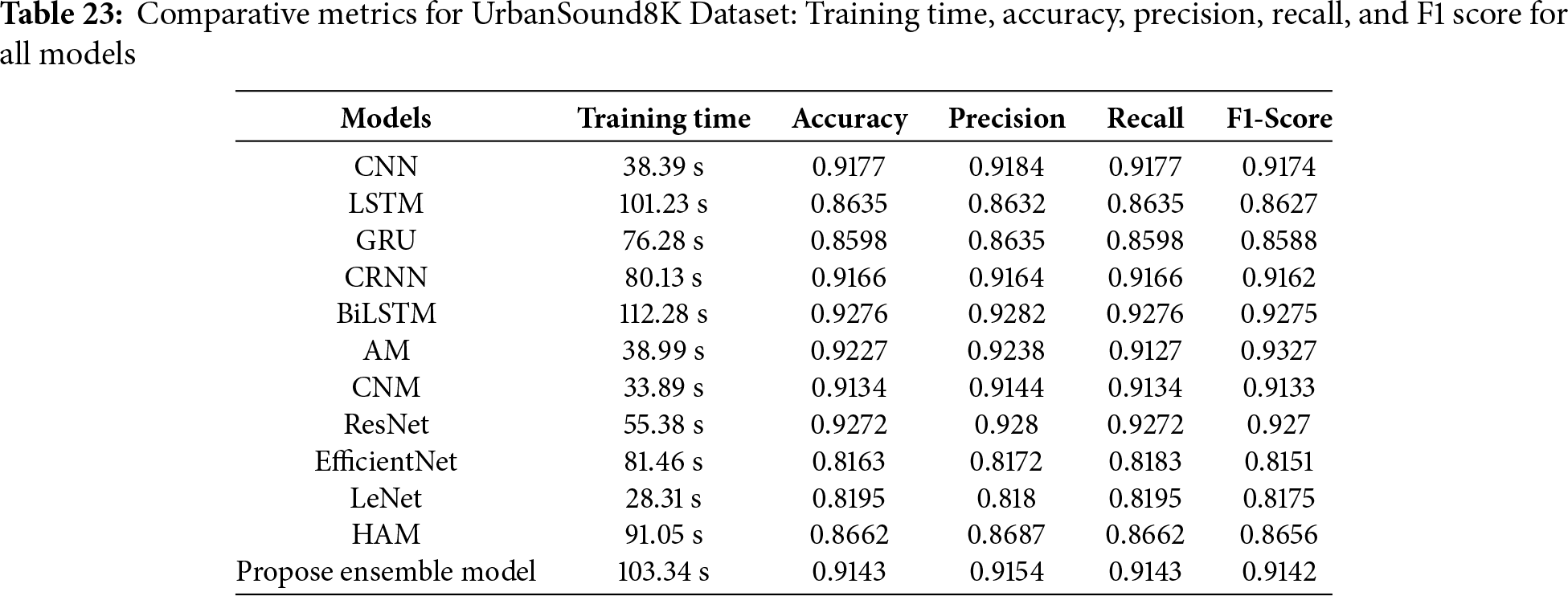
4.18 Comparative Analysis of All Models with UrbanSound8K Dataset

The results of each model utilized in this study are displayed in Table 23. CNN, LSTM, GRU, CRNN, BiLSTM, AM, CNM, ResNet, EfficientNet, LeNet, and HAM models have all been improved to yield the best results with the provided dataset; nonetheless, the proposed model performs better than any of them. The suggested model, however, outperforms all the already used models. Hyperparameters in DL can be chosen via hyperparameter optimization techniques, or they can be given by the user. DL models can be fine-tuned using these parameters to obtain better accuracy. The learning process itself is impacted by hyperparameters, in contrast to the model parameters, which are learnt during the training phase.

4.19 Performance Comparison with Existing Approaches

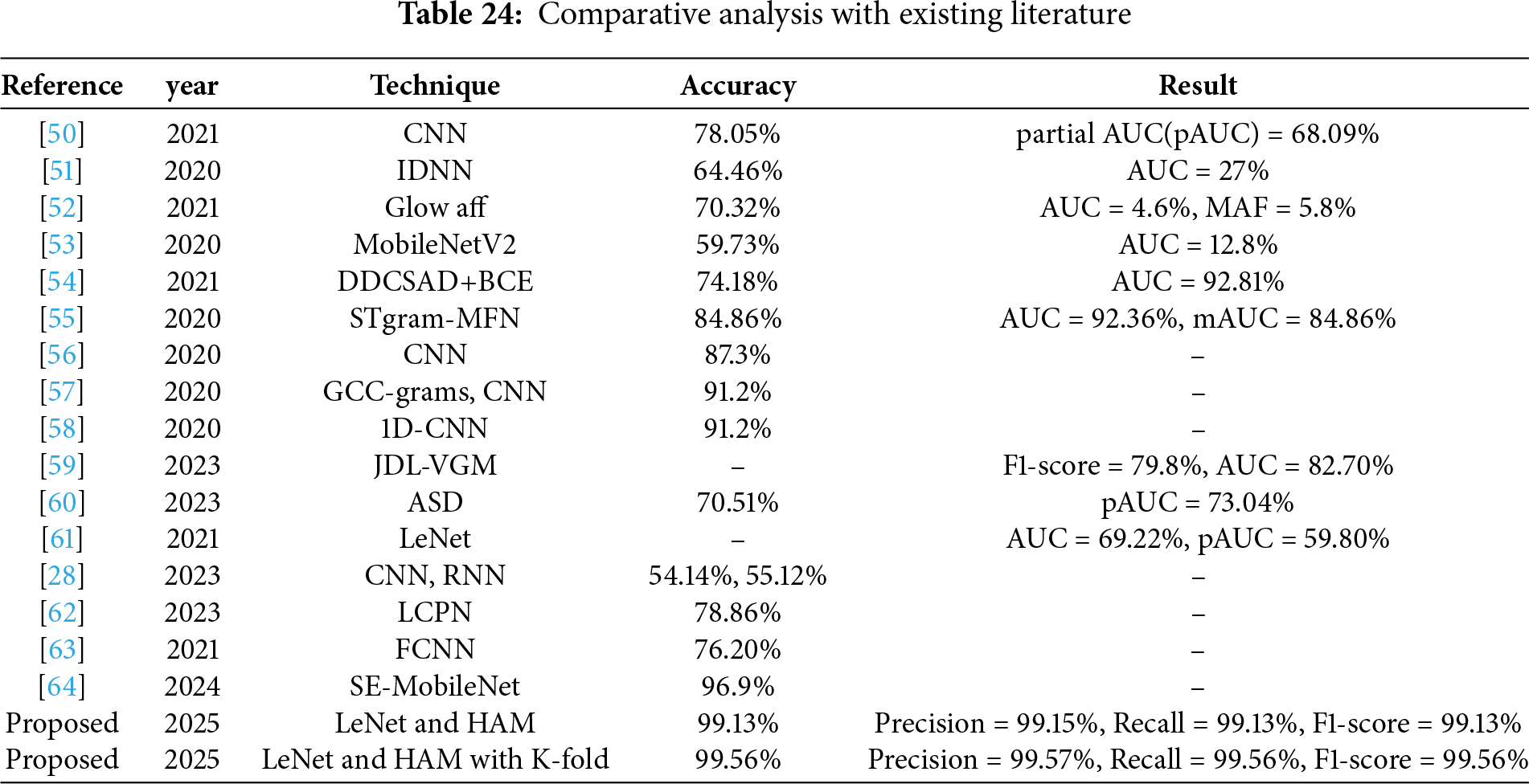
Several models from the corpus of studies that employed DL algorithms for audio classification are compared to one another. These studies were selected because they used the same dataset for trials and because they may be used as a reference to evaluate how well the proposed ensemble model works. Table 24 highlights the disparities in performance across the different deep learning models and shows that the LeNet and HAM model performs better.

5  Conclusion

This study proposes an ensemble deep learning (DL) approach for car fault detection using engine sounds. The utilization of numerous DL models, including GRU, LSTM, CNN, CRNN, AM, BiLSTM, CNM, ResNet, EfficientNet, HAM, and LeNet, has been investigated for audio classification. With an accuracy of 99.13%, the ensemble LeNet and HAM model is the most accurate one and demonstrates the potential of CNNs for audio classification problems. As per the experimental findings, LeNet and HAM performed better than HAM, with an accuracy of 99.13% and a k-fold cross-validation accuracy of 99.56%, where k is 3, 5, 7, and 10, respectively. However, as the examination of these models progressed, the challenge of distinguishing anomalies from normal audio patterns became evident. Identifying anomalies in audio signals remains a complex task, necessitating further research to enhance the robustness of models in detecting and classifying such deviations. The refinement and optimization of deep learning models for audio classification will require a nuanced approach, particularly in addressing the intricacies of anomaly detection. Further research in this domain is pivotal for developing more reliable and accurate audio processing systems.

Acknowledgement: The authors would like to express their gratitude to Princess Nourah bint Abdulrahman University Researchers Supporting Project number (PNURSP2025R746), Princess Nourah bint Abdulrahman University, Riyadh, Saudi Arabia.

Funding Statement: This research was funded by Princess Nourah bint Abdulrahman University Researchers Supporting Project number (PNURSP2025R746), Princess Nourah bint Abdulrahman University, Riyadh, Saudi Arabia.

Author Contributions: Mudasir Ali conceived the idea, performed data analysis and wrote the original draft. Muhammad Faheem Mushtaq conceived the idea, performed data curation and wrote the original draft. Urooj Akram performed data curation, formal analysis, and designed methodology. Nagwan Abdel Samee acquired the funding for research, and performed visualization and initial investigation. Mona M. Jamjoom dealt with software, performed visualization and carried out project administration. Imran Ashraf supervised the study, performed validation and review and edit the manuscript. All authors reviewed the results and approved the final version of the manuscript.

Availability of Data and Materials: The data can be requested from the corresponding authors.

Ethics Approval: Not applicable.

Conflicts of Interest: The authors declare no conflicts of interest to report regarding the present study.

References

1. De Benito-Gorrón D, Ramos D, Toledano DT. A multi-resolution CRNN-based approach for semi-supervised sound event detection in DCASE, 2020 challenge. IEEE Access. 2021;9:89029–42. doi:10.1109/access.2021.3088949. [Google Scholar] [CrossRef]

2. Morato IM, Heittola T, Mesaros A, Virtanen T. Low-complexity acoustic scene classification for multi-device audio: analysis of DCASE, 2021 challenge systems. In: Proceedings of the Detection and Classication of Acoustic Scenes and Events; 2021 Nov 15–19; Online. p. 85–9. [Google Scholar]

3. Wang S, Heittola T, Mesaros A, Virtanen T. Audio-visual scene classification: analysis of DCASE, 2021 challenge submissions. arXiv:2105.13675. 2021. [Google Scholar]

4. Su Y, Zhang K, Wang J, Madani K. Environment sound classification using a two-stream CNN based on decision-level fusion. Sensors. 2019;19(7):1733. doi:10.3390/s19071733. [Google Scholar] [PubMed] [CrossRef]

5. Wang Q, Zheng S, Li Y, Wang Y, Wu Y, Hu H, et al. A model ensemble approach for audio-visual scene classification. In: Proceedings of the 6th Workshop on Detection and Classification of Acoustic Scenes and Events; 2021 Nov 15–19; Online. Park Avenue, New York City, NY, USA. [Google Scholar]

6. Sun K, Zhang J, Zhang C, Hu J. Generalized extreme learning machine autoencoder and a new deep neural network. Neurocomputing. 2017;230:374–81. doi:10.1016/j.neucom.2016.12.027. [Google Scholar] [CrossRef]

7. Liu W, Wang Z, Liu X, Zeng N, Liu Y, Alsaadi FE. A survey of deep neural network architectures and their applications. Neurocomputing. 2017;234:11–26. doi:10.1016/j.neucom.2016.12.038. [Google Scholar] [CrossRef]

8. Müller R, Ritz F, Illium S, Linnhoff-Popien C. Acoustic anomaly detection for machine sounds based on image transfer learning. arXiv:2006.03429. 2020. [Google Scholar]

9. Ioffe S, Szegedy C. Batch normalization: accelerating deep network training by reducing internal covariate shift. In: International Conference on Machine Learning. Westminster, UK: PMLR; 2015. p. 448–56. [Google Scholar]

10. Abeßer J. A review of deep learning based methods for acoustic scene classification. Appl Sci. 2020;10(6):2020. doi:10.3390/app10062020. [Google Scholar] [CrossRef]

11. Duman TB, Bayram B, İnce G. Acoustic anomaly detection using convolutional autoencoders in industrial processes. In: 14th International Conference on Soft Computing Models in Industrial and Environmental Applications (SOCO 2019); 2019 May 13–15; Seville, Spain. Cham, Switzerland: Springer; 2020. p. 432–42. [Google Scholar]

12. Koizumi Y, Saito S, Uematsu H, Harada N. Optimizing acoustic feature extractor for anomalous sound detection based on Neyman-Pearson lemma. In: 2017 25th European Signal Processing Conference (EUSIPCO); 2017 Aug 28–Sep 2; Kos Island, Greece: IEEE. p. 698–702. [Google Scholar]

13. Marchi E, Vesperini F, Eyben F, Squartini S, Schuller B. A novel approach for automatic acoustic novelty detection using a denoising autoencoder with bidirectional LSTM neural networks. In: 2015 IEEE International Conference on Acoustics, Speech and Signal Processing (ICASSP); 2015 Apr 19–24; South Brisbane, QLD, Australia. p. 1996–2000. [Google Scholar]

14. Bayram B, Duman TB, Ince G. Real time detection of acoustic anomalies in industrial processes using sequential autoencoders. Expert Syst. 2021;38(1):e12564. doi:10.1111/exsy.12564. [Google Scholar] [CrossRef]

15. Kawaguchi Y, Tanabe R, Endo T, Ichige K, Hamada K. Anomaly detection based on an ensemble of dereverberation and anomalous sound extraction. In: ICASSP 2019-2019 IEEE International Conference on Acoustics, Speech and Signal Processing (ICASSP); 2019 May 12–17; Brighton, UK. p. 865–9. [Google Scholar]

16. Koizumi Y, Murata S, Harada N, Saito S, Uematsu H. SNIPER: few-shot learning for anomaly detection to minimize false-negative rate with ensured true-positive rate. In: ICASSP 2019-2019 IEEE International Conference on Acoustics, Speech and Signal Processing (ICASSP); 2019 May 12–17; Brighton, UK. p. 915–9. [Google Scholar]

17. Hayashi T, Komatsu T, Kondo R, Toda T, Takeda K. Anomalous sound event detection based on wavenet. In: 2018 26th European Signal Processing Conference (EUSIPCO); 2018 Sep 3–7; Rome, Italy: IEEE. p. 2494–8. [Google Scholar]

18. Rushe E, Mac Namee B. Anomaly detection in raw audio using deep autoregressive networks. In: ICASSP 2019-2019 IEEE International Conference on Acoustics, Speech and Signal Processing (ICASSP); 2019 May 12–17; Brighton, UK. p. 3597–601. [Google Scholar]

19. Avd O, Dieleman S, Zen H, Simonyan K, Vinyals O, Graves A, et al. Wavenet: a generative model for raw audio. arXiv:1609.03499. 2016. [Google Scholar]

20. Huzaifah M. Comparison of time-frequency representations for environmental sound classification using convolutional neural networks. arXiv:1706.07156. 2017. [Google Scholar]

21. Zinemanas P, Cancela P, Rocamora M. End-to-end convolutional neural networks for sound event detection in urban environments. In: 2019 24th Conference of Open Innovations Association (FRUCT); 2019 Apr 8–12; Moscow, Russia. p. 533–9. [Google Scholar]

22. Mendoza JM, Tan V, Fuentes V, Perez G, Tiglao NM. Audio event detection using wireless sensor networks based on deep learning. In: Wireless Internet: 11th EAI International Conference, WiCON 2018; 2018 Oct 15–16; Taipei, Taiwan. Cham, Switzerland: Springer; 2019. p. 105–15. [Google Scholar]

23. Lhoest L, Lamrini M, Vandendriessche J, Wouters N, da Silva B, Chkouri MY, et al. Mosaic: a classical machine learning multi-classifier based approach against deep learning classifiers for embedded sound classification. Appl Sci. 2021;11(18):8394. doi:10.3390/app11188394. [Google Scholar] [CrossRef]

24. Piczak KJ. Environmental sound classification with convolutional neural networks. In: 2015 IEEE 25th International Workshop on Machine Learning for Signal Processing (MLSP); 2015 Sep 17–20; Boston, MA, USA. p. 1–6. doi:10.1109/mlsp.2015.7324337. [Google Scholar] [CrossRef]

25. Piczak KJ. ESC: dataset for environmental sound classification. In: Proceedings of the 23rd ACM International Conference on Multimedia; 2015 Oct 26–30; Brisbane, QLD, Australia. p. 1015–8. [Google Scholar]

26. Shah SK, Tariq Z, Lee Y. IoT based urban noise monitoring in deep learning using historical reports. In: 2019 IEEE International Conference on Big Data (Big Data); 2019 Dec 9–12; Los Angeles, CA, USA. p. 4179–84. [Google Scholar]

27. Vandendriessche J, Wouters N, da Silva B, Lamrini M, Chkouri MY, Touhafi A. Environmental sound recognition on embedded systems: from fpgas to tpus. Electronics. 2021;10(21):2622. doi:10.3390/electronics10212622. [Google Scholar] [CrossRef]

28. Singh VK, Sharma K, Sur SN. Development of acoustic scene classification model using neural networks applied on reduced dataset of dcase. In: 2023 9th International Conference on Signal Processing and Communication (ICSC); 2023 Dec 21–23; Noida, India. p. 544–50. [Google Scholar]

29. Sony S, Gamage S, Sadhu A, Samarabandu J. Multiclass damage identification in a full-scale bridge using optimally tuned one-dimensional convolutional neural network. J Comput Civ Eng. 2022;36(2):04021035. doi:10.1061/(asce)cp.1943-5487.0001003. [Google Scholar] [CrossRef]

30. Shim H, Kim J, Jung J, Yu Hj. Audio tagging and deep architectures for acoustic scene classification: UOS submission for the DCASE, 2020 challenge. In: Proceedings of the DCASE2020 Challenge; 2020 Nov 2–4; Park Avenue, New York City, NY, USA. [Google Scholar]

31. Lu Y, Huang Z. A new hybrid model of sparsity empirical wavelet transform and adaptive dynamic least squares support vector machine for fault diagnosis of gear pump. Adv Mech Eng. 2020;12(5):1687814020922047. doi:10.1177/1687814020922047. [Google Scholar] [CrossRef]

32. Pablo Fernández J, Shubitidze F, Shamatava I, Barrowes BE, O’Neill K. Realistic subsurface anomaly discrimination using electromagnetic induction and an SVM classifier. EURASIP J Adv Sig Process. 2010;2010(1):1–11. doi:10.1155/2010/305890. [Google Scholar] [CrossRef]

33. Glowacz A, Tadeusiewicz R, Legutko S, Caesarendra W, Irfan M, Liu H, et al. Fault diagnosis of angle grinders and electric impact drills using acoustic signals. Appl Acoust. 2021;179:108070. doi:10.1016/j.apacoust.2021.108070. [Google Scholar] [CrossRef]

34. Ahn H, Choi HL, Kang M, Moon S. Learning-based anomaly detection and monitoring for swarm drone flights. Appl Sci. 2019;9(24):5477. doi:10.3390/app9245477. [Google Scholar] [CrossRef]

35. Ahn H, Jung D, Choi HL. Deep generative models-based anomaly detection for spacecraft control systems. Sensors. 2020;20(7):1991. doi:10.3390/s20071991. [Google Scholar] [PubMed] [CrossRef]

36. Malhotra P, Ramakrishnan A, Anand G, Vig L, Agarwal P, Shroff G. LSTM-based encoder-decoder for multi-sensor anomaly detection. arXiv:1607.00148. 2016. [Google Scholar]

37. Koizumi Y, Saito S, Uematsu H, Kawachi Y, Harada N. Unsupervised detection of anomalous sound based on deep learning and the neyman-pearson lemma. IEEE/ACM Transact Audio Speech Lang Process. 2018;27(1):212–24. doi:10.1109/taslp.2018.2877258. [Google Scholar] [CrossRef]

38. Chauhan S, Vig L. Anomaly detection in ECG time signals via deep long short-term memory networks. In: 2015 IEEE International Conference on Data Science and Advanced Analytics (DSAA); 2015 Oct 19–21; Paris, France. p. 1–7. [Google Scholar]

39. Malhotra P, Vig L, Shroff G, Agarwal P. Long short term memory networks for anomaly detection in time series. In: ESANN 2015 Proceedings, European Symposium on Artificial Neural Networks, Computational Intelligence and Machine Learning; 2015 Apr 22–24; Bruges, Belgium. p. 89–94. [Google Scholar]

40. Gers FA, Schmidhuber J, Cummins F. Learning to forget: continual prediction with LSTM. Neural Comput. 2000;12(10):2451–71. doi:10.1162/089976600300015015. [Google Scholar] [PubMed] [CrossRef]

41. Zhu Y, Bao W, Yu Q. Towards open set video anomaly detection. In: European Conference on Computer Vision. Cham, Switzerland: Springer; 2022. p. 395–412. [Google Scholar]

42. Peng T, Qiu R, Zhu J, Xiao Y, Wang S, Zhang Y, et al. Unsupervised abnormal sound detection based on spectral coherence and feature fusion in domain displacement condition. In: Detection and Classification of Acoustic Scenes and Events 2022; 2022. [Google Scholar]

43. Shi X, Chen Z, Wang H, Yeung DY, Wong WK, Wc Woo. Convolutional LSTM network: a machine learning approach for precipitation nowcasting. In: Advances in neural information processing systems. Cambridge, MA, USA: MIT Press; 2015. 28 p. [Google Scholar]

44. Bojanowski P, Grave E, Joulin A, Mikolov T. Enriching word vectors with subword information. Transact Associat Computat Linguist. 2017;5(1):135–46. doi:10.1162/tacl_a_00051. [Google Scholar] [CrossRef]

45. Maya S, Ueno K, Nishikawa T. dLSTM: a new approach for anomaly detection using deep learning with delayed prediction. Int J Data Sci Analyt. 2019;8:137–64. doi:10.1007/s41060-019-00186-0. [Google Scholar] [CrossRef]

46. Le NQK, Do DT, Hung TNK, Lam LHT, Huynh TT, Nguyen NTK. A computational framework based on ensemble deep neural networks for essential genes identification. Int J Mol Sci. 2020;21(23):9070. doi:10.3390/ijms21239070. [Google Scholar] [PubMed] [CrossRef]

47. Hu J, Shen L, Sun G. Squeeze-and-excitation networks. In: Proceedings of the IEEE Conference on Computer Vision and Pattern Recognition; 2018 Jun 18–23; Salt Lake City, UT, USA. p. 7132–41. [Google Scholar]

48. Vaswani A, Shazeer N, Parmar N, Uszkoreit J, Jones L, Gomez AN, et al. Attention is all you need. In: Advances in neural information processing systems. Cambridge, MA, USA: MIT Press; 2017. 30 p. [Google Scholar]

49. Kong Q, Cao Y, Iqbal T, Wang Y, Wang W, Plumbley MD. Panns: large-scale pretrained audio neural networks for audio pattern recognition. IEEE/ACM Transact Audio Speech Lang Process. 2020;28:2880–94. doi:10.1109/taslp.2020.3030497. [Google Scholar] [CrossRef]

50. Morita K, Yano T, Tran K. Anomalous sound detection using CNN-based features by self supervised learning. In: Detection and Classification of Acoustic Scenes and Events 2021; 2021. [Google Scholar]

51. Suefusa K, Nishida T, Purohit H, Tanabe R, Endo T, Kawaguchi Y. Anomalous sound detection based on interpolation deep neural network. In: ICASSP 2020-2020 IEEE International Conference on Acoustics, Speech and Signal Processing (ICASSP); 2020 May 4–9; Park Avenue, New York City, NY, USA. p. 271–5. [Google Scholar]

52. Dohi K, Endo T, Purohit H, Tanabe R, Kawaguchi Y. Flow-based self-supervised density estimation for anomalous sound detection. In: ICASSP 2021-2021 IEEE International Conference on Acoustics, Speech and Signal Processing (ICASSP); 2021 Jun 6–11; Toronto, ON, Canada. p. 336–40. [Google Scholar]

53. Giri R, Tenneti SV, Cheng F, Helwani K, Isik U, Krishnaswamy A. Self-supervised classification for detecting anomalous sounds. In: Detection and Classification of Acoustic Scenes and Events 2020; 2020 Nov 2–3; Tokyo, Japan. [Google Scholar]

54. Kuroyanagi I, Hayashi T, Takeda K, Toda T. Anomalous sound detection using a binary classification model and class centroids. In: 2021 29th European Signal Processing Conference (EUSIPCO); 2021 Aug 23–27; Dublin, Ireland. p. 1995–9. [Google Scholar]

55. Liu Y, Guan J, Zhu Q, Wang W. Anomalous sound detection using spectral-temporal information fusion. In: ICASSP 2022-2022 IEEE International Conference on Acoustics, Speech and Signal Processing (ICASSP); 2022 May 23–27; Singapore. p. 816–20. [Google Scholar]

56. Heittola T, Mesaros A, Virtanen T. Acoustic scene classification in dcase 2020 challenge: generalization across devices and low complexity solutions. arXiv:2005.14623. 2020. [Google Scholar]

57. LopezMeyer P, Ontiveros JDH, Lu H, Corcourier H, Stemmer G, Nachman L, et al. Low-memory convolutional neural networks for acoustic scene classification. In: Detection and Classification of Acoustic Scenes and Events 2020; 2020. [Google Scholar]

58. Pajusco N, Huang R, Farrugia N. Lightweight convolutional neural networks on binaural waveforms for low complexity acoustic scene classification. In: Detection and Classification of Acoustic Scenes and Events 2020; 2020 Nov 2–3; Tokyo, Japan. p. 135–9. [Google Scholar]

59. Bi Z, Li H, Zhang W, Dong Z. Variational bayesian clustering algorithm for unsupervised anomalous sound detection incorporating VH-BCL+. Multimed Tools Appl. 2024;83:43777–800. doi:10.1007/s11042-023-17006-0. [Google Scholar] [CrossRef]

60. Zhou H, Wang K, Yao J, Yang W, Chai Y. Anomaly sound detection of industrial equipment based on incremental learning. In: 2023 CAA Symposium on Fault Detection, Supervision and Safety for Technical Processes (SAFEPROCESS); 2023 Sep 22–24; Yibin, China. p. 1–6. [Google Scholar]

61. Pham L, Jalali A, Dinica O, Schindler A. DCASE challenge 2021: unsupervised anomalous sound detection of machinery with LeNet architecture. In: Detection and Classification of Acoustic Scenes and Events 2021; 2021. [Google Scholar]

62. Ding B, Zhang T, Liu G, Wang C. Hierarchical classification for acoustic scenes using deep learning. Appl Acoust. 2023;212:109594. doi:10.1016/j.apacoust.2023.109594. [Google Scholar] [CrossRef]

63. Hu H, Yang CHH, Xia X, Bai X, Tang X, Wang Y, et al. A two-stage approach to device-robust acoustic scene classification. In: ICASSP 2021-2021 IEEE International Conference on Acoustics, Speech and Signal Processing (ICASSP); 2021 Jun 6–11; Toronto, ON, Canada. p. 845–9. [Google Scholar]

64. Spoorthy V, Koolagudi SG. Bi-level acoustic scene classification using lightweight deep learning model. Circ Syst Signal Process. 2024;43(1):388–407. doi:10.1007/s00034-023-02478-0. [Google Scholar] [CrossRef]