
 Submit a Paper
 Propose a Special lssue
 Open Access
ARTICLE

Graph Neural Network-Assisted Lion Swarm Optimization for Traffic Congestion Prediction in Intelligent Urban Mobility Systems
1 Department of Electrical Engineering, College of Engineering, Jouf University, Sakakah, 72388, Saudi Arabia
2 Department of Interior Design, College of Engineering, Jouf University, Sakakah, 72388, Saudi Arabia
3 Department of Electrical Engineering, College of Engineering, University of Hafr Al Batin, Hafr Al Batin, 39524, Saudi Arabia
4 Institute for Intelligent Systems and Robotics (ISIR), CNRS, Sorbonne University, Paris, 75006, France
5 Electrical Engineering Department, University of Business and Technology, Ar Rawdah, Jeddah, 23435, Saudi Arabia
6 Engineering Mathematics Department, Alexandria University, Lotfy El-Sied st. off Gamal Abd El-Naser, Alexandria, 11432, Egypt
* Corresponding Author: Gehan Elsayed. Email:
(This article belongs to the Special Issue: Machine Learning and Deep Learning-Based Pattern Recognition)
Computer Modeling in Engineering & Sciences 2025, 145(2), 2277-2309. https://doi.org/10.32604/cmes.2025.070726
Received 22 July 2025; Accepted 11 October 2025; Issue published 26 November 2025
 View Full Text
 Download PDF
Abstract
Traffic congestion plays a significant role in intelligent transportation systems (ITS) due to rapid urbanization and increased vehicle concentration. The congestion is dependent on multiple factors, such as limited road occupancy and vehicle density. Therefore, the transportation system requires an effective prediction model to reduce congestion issues in a dynamic environment. Conventional prediction systems face difficulties in identifying highly congested areas, which leads to reduced prediction accuracy. The problem is addressed by integrating Graph Neural Networks (GNN) with the Lion Swarm Optimization (LSO) framework to tackle the congestion prediction problem. Initially, the traffic information is collected and processed through a normalization process to scale the data and mitigate issues of overfitting and high dimensionality. Then, the traffic flow and temporal characteristic features are extracted to identify the connectivity of the road segment. From the connectivity and node relationship graph, modeling improves the overall prediction accuracy. During the analysis, the lion swarm optimization process utilizes the concepts of exploration and exploitation to understand the complex traffic dependencies, which helps predict high congestion on roads with minimal deviation errors. There are three core optimization phases: roaming, hunting, and migration, which enable the framework to make dynamic adjustments to enhance the predictions. The framework’s efficacy is evaluated using benchmark datasets, where the proposed work achieves 99.2% accuracy and minimizes the prediction deviation value by up to 2.5% compared to other methods. With the new framework, there was a more accurate prediction of real-time congestion, lower computational cost, and improved regulation of traffic flow. This system is easily implemented in intelligent transportation systems, smart cities, and self-driving cars, providing a robust and scalable solution for future traffic management.Keywords
1.1 Understanding Traffic Congestion: Causes, Occurrence, and Impact
The sustained critical challenge in modern Intelligent Transportation Systems (ITS) [1] is traffic congestion, which affects urban mobility and transport sustainability [2], particularly at the system level. Over time, as cities continue to expand rapidly, the number of vehicles increases, resulting in delays, higher fuel consumption, and increased pollution. One of the problems in metropolitan areas is vehicular traffic congestion [3], which is exacerbated by the increasing number of vehicles resulting from urbanization and population growth. It leads to significant improvements in travel time, but also increased fuel consumption and lower air quality. The resulting overload [4] of road networks causes delays and inefficient development of transportation systems. The discussed obstacles affect not only commuters but also public transport operations [5], logistics, emergency response integration, and many other essential aspects of orderly city life. The congestion [6] causes issues like road capacity, accidents, traffic density, and spontaneous travel demand. In heavily populated cities, the tipping point that leads to a traffic jam [7] is much lower due to the large number of people, which can lead to chain reactions. One of the main goals for peak-time mobility is to resolve traffic congestion as quickly as possible, conserve the environment by reducing fuel consumption and vehicle emissions, and minimize economic damages. The imbalance [8] between demand and the available infrastructure causes differences between user expectations and traffic congestion. Once the number of vehicles exceeds the capacity of a road, mobility [9] is drastically reduced, further slowing down the movement of traffic. Urbanization, rapid population growth, inadequate infrastructure development, excessive road usage, and uncoordinated traffic signals are key factors contributing to congestion. Additionally, external factors [10] such as accidents, road-related maintenance work, harsh weather conditions, and increased demand during specific seasons or holidays contribute to congestion. Some other reasons that lead to traffic flow [11] disruption are sudden braking, lane shifting, and aggressive vehicle driving, which force vehicular movement to alternate from stationary to slow-moving and repeat the cycle.
Congestion occurs when the number of vehicles on the road exceeds the designated capacity, causing trapped cars to travel at an exceptionally slow pace and take longer to reach their destination. It typically begins when vehicles enter a roadway at a velocity exceeding the exit capacity, resulting in a queue of automobiles. This obstruction phenomenon can spread throughout a network, exacerbating congestion over time. Congestion [12] is further developed when a vehicle decelerates due to an obstruction or a traffic control device. Vehicles that follow behind now need to decelerate, creating a lag-induced delay termed the shockwave effect in traffic. In urban regions [13], these small changes, such as lane blockages or variations in pedestrian crossing types, can lead to widespread traffic congestion.
In contrast, non-recurrent congestion [14,15] is defined as congestion that occurs due to unforeseen issues, such as vehicular crashes or unfavorable climatic conditions. Expressive congestion occurs during certain times of the day owing to high commuting traffic. All of these factors contribute to the heavy congestion of traffic, which collectively reduces the effectiveness of transportation.
1.2 Solutions to Traffic Congestion: Effective Strategies and Approaches
A combination of these different measures, such as adopting new technologies [16], increasing public spending, and properly supervising traffic, can help other places relieve vehicular congestion. The construction of over- and underpasses, additional lanes, and road circumventions ensures an adequate supply of road space to accommodate increased traffic volume. The adaptive control of traffic signals and thorough monitoring of vehicular movement help manage the flow of vehicles and minimize standstill traffic problems [17]. Extensions in public transport systems, such as improved buses, metros, and enhanced cycling paths, all help broaden the scope of travel, which in turn reduces the use of cars and other privately owned means of transport. Conventional traffic management methods, such as rule-based control of traffic signals and static routing systems, fail to keep pace with the inherently complex and dynamic nature of real-life traffic performance. These methods have been improved with the advent of IoT, V2X communication, and Artificial intelligence systems, improving the overall functionality of intelligent transport systems.
1.3 Key Challenges in Traffic Management Systems
Even with the added technologies of V2X communication, AI, and GNN integrated with an ITS, traffic supervision challenges continue to persist. One major challenge has been the scalability and real-time adaptability of these systems in a fast-paced, dense metropolitan city. Existing models cannot accurately predict and provide adaptive control due to unpredictable incidents, such as sudden changes in weather, unexpected increases in traffic volume, and unforeseen accidents. Additionally, the heterogeneity of data sources, including GPS systems, sensors, and connected vehicles, creates challenges in data fusion and synchronization, resulting in inefficiencies in data processing and decision-making.
Furthermore, the need for infrastructure deployment and maintenance, such as upgrading road networks with sensors, alongside the addition of 5G-enabled V2X communication, proves too costly, especially for developing regions, resulting in limited popularity of these systems. The non-compliance with the devised intelligent traffic suggestions and reluctance to share mobility solutions provided by the city pose human behavioral factors that reverse the intended effect of congestion mitigation plans. Tackling these challenges requires further progress in predictive analytics, secure and scalable intelligent traffic system architectures, and relevant policy measures to enable the integration of smart traffic management systems. Congestion prediction, which combines traffic speed/flow regression with congestion classification, is the primary focus of this research. Secondary applications, such as adaptive control and route optimization, utilize projected congestion conditions to inform their decisions. The GNN-LSO methodology can feed into downstream control schemes, but its primary contribution is the accurate and scalable prediction of traffic congestion. These problems are addressed by introducing the following contributions listed below.
• To integrate Graph Neural Networks with Lion Swarm Optimization for accurate traffic prediction and congestion prediction.
• Through adaptive optimization, reduce prediction errors and improve robustness and dependability under different traffic situations.
• To enhance computing efficiency, utilize metaheuristic optimization to expedite convergence and facilitate real-time deployment.
• To ensure scalability across various datasets, validate the system on multiple urban and highway traffic scenarios to demonstrate its adaptability.
• To integrate spatio-temporal graph learning and swarm-based optimization to balance accuracy, stability, and computational cost in intelligent transportation systems.
The paper is structured as follows: Section 2 discusses the various opinions of researchers on traffic congestion prediction. Section 3 explains the working process of the GNN with the LSO framework for identifying traffic congestion in a dynamic environment. Section 4 estimates the system’s efficiency, and the conclusion is described in Section 5.
Bai et al. (2021) address the issue of precision traffic congestion forecasting in smart cities by proposing the PrePCT model [18], which incorporates spatial and temporal dependencies among road segments. The objective of this study is to enhance congestion prediction by incorporating relative positional relationships into tensor structure modeling. The model utilizes deep learning, specifically convolutional networks with long-range capabilities, to analyze historical congestion and regional spatial data, enabling accurate traffic predictions. Although this method outperforms traditional methods, some drawbacks include potential scalability issues with extensive road networks and vulnerability to data sparsity in low-density traffic areas.
The latest research from Mehdi and others (2022) [19] suggests an entropy-based traffic flow labeling approach to enhance CNN-based traffic congestion prediction using its meta–parameters. The study examines how labeling with entropy can improve classification accuracy despite the set of labeled data that defines its data representation for deep learning models. The method combines traffic flow characteristics with the dynamics of entropy categorization to enable CNNs to discern different congestion levels. Although the system has enhanced prediction performance, challenges include dependence on the correct and accurate selection of the meta-parameter, as well as extreme changes in traffic patterns that can cause severe sensitivity, thereby impacting real-time processing in densely populated metropolitan areas.
Chen et al. (2024) [20] aim to advance traffic flow forecasting using the TFM-GNN model, which incorporates an attention mechanism to model spatial-temporal dependencies more effectively. The author includes an attention mechanism that enhances the structured graph representation of traffic data and identifies the most critical road segments. Their approach captures the traffic flow matrix, uses graph neural networks (GNNs), and predicts correlations with higher accuracy using node-averaged road models. Even with the improved efficiency compared to traditional models, the system faces several difficulties, including the high sensitivity of computation in large-scale networks and the lack of real-time applicability due to missing or inconsistent traffic data.
Tu et al. (2021) [21] present a novel approach for predicting traffic congestion by utilizing deep learning methods in conjunction with road segment clustering to improve the accuracy of predictions. In this study, the goal is to enhance congestion prediction by merging road segments that share comparable traffic flow patterns, enabling deeper levels of the model to capture spatial-temporal relationships more effectively. The introduced technique employs a hybrid approach combining CNNs and LSTMs, where CNNs spatially localize features from previous epochs. The LSTM processes the spatial feature dynamics in different time frames, making the predictions more accurate. The model is better than the standard models, but group segmentation for optimization and scaling to large metropolitan road networks tends to be inefficient.
Gao et al. (2021) [22] suggest using an image-based approach to a CNN for traffic congestion estimation, focusing on traffic data as images. The aim is to improve congestion prediction accuracy by leveraging the strong feature extraction ability of CNNs, treating video images of traffic flows as input for deep learning processes. The CNN approach converts traditional numeric traffic information into grid images that can be processed by CNNs, capturing congestion patterns and their spatial dependencies. Although the approach improves estimation accuracy, some tradeoff factors include the loss of complex, detailed information in temporal patterns, and processing high-dimensional traffic image data comes with the cost of computational power.
The goal of Faridai et al. (2021) [23] aims to enhance public transport traffic management by predicting passenger congestion using deep learning techniques, which help improve the efficiency of scheduling and resource allocation. For the task, they utilized a neural network trained on historical passenger flow data, enabling the system to recognize patterns and dynamically predict congestion, thereby optimizing transport lines. The model does improve public transport mobility planning; however, it is limited by being potentially oversensitive to sudden demand shifts and relying heavily on extensive, high-quality datasets of passenger flow for accurate predictions.
Bharti et al. (2023) [24] developed a deep learning-based short-term traffic flow prediction model, specifically a Bi-LSTM model with hyperparameters tuned using Particle Swarm Optimization (PSO). The goal is to increase prediction accuracy by adjusting the hyperparameters of the Bi-LSTM model to make it more adaptive to changing traffic conditions using PSO. The approach utilizes the bidirectional feature of Bi-LSTM to capture both past and future traffic data dependencies, while the PSO algorithm optimizes the model parameters to achieve better results. Although it is effective, some issues remain, including high computational complexity and difficulties in real-time implementation due to the optimization iterations.
Hussain and others (2021) utilize an optimized Gated Recurrent Unit (GRU) model for forecasting traffic efficiently. The research aims to optimize the model’s hyperparameters to capture the non-linear, complex dependencies of traffic data over time. This method utilizes metaheuristic optimization methods in the GRU structure, guaranteeing better performance than most recurrent models. Although the model achieves better accuracy, efficiency, and reduced computation, challenges remain related to its sensitivity to extreme traffic patterns and the need for extensive training data to perform well in different cities.
Dikshit et al. (2023) [25] consider the problem of traffic congestion and describe how AI can be employed in optimizing vehicle routing in urban centers. The goal is to enhance flow efficiency by utilizing AI-based solutions that automatically adjust routes based on the dynamic traffic conditions of a given city. The AI approach uses machine learning and heuristic optimization methods to predict road congestion and recommend the most efficient vehicle routing strategies. Although the model enhances the mobility of urban areas and reduces travel time, it has two drawbacks: a dependency on accurate real-time traffic data and cumbersome computation requirements for large-scale dynamic routing optimization.
Djenouri et al. (2023) [26] propose a novel approach that combines a hybrid Graph Convolutional Neural Network (GCN) with Branch-and-Bound (B&B) optimization for traffic flow forecasting, emphasizing both accuracy and computational efficiency. In this study, GCNs spatially comprehend the dependencies in a road network, while the B&B optimization sequentially solves the remaining solution space to increase accuracy. The proposed method integrates deep learning and combinatorial optimization, which improves the predictive power of traffic flow forecasting. On the other hand, the drawbacks include the expensive requirements for training GCNs on larger networks and the potential for incomplete or inaccurate data regarding traffic.
Yang et al. (2021) [27] propose an SA-enhanced ARIMA-BP neural network model for predicting network traffic, combining deep learning and statistical methods to achieve improved accuracy. Combining ARIMA with Back Propagation (BP) neural networks enables the capture of linear traffic flow patterns while modeling non-linear tendencies, and hyperparameter tuning improves the convergence speed with SA. This hybrid system captures precision in short-term forecasts while accommodating fluctuating traffic ranges. Despite its shortcomings, including inadequacy in processing highly volatile traffic and the additional computation required for SA optimization, it remains effective.
Bakirci [28] compared the YOLOv8n algorithm for real-time vehicle recognition on a UAV platform with other variations to determine the performance balance. Object detection and density mapping at critical transport nodes were performed using a bespoke traffic dataset from UAV-mounted cameras. Fast Jetson Nano detection and 0.706 precision provided reliable vehicle tracking and trajectory mapping. However, low precision relative to later YOLO variants and UAV stability remain significant issues. To achieve transparent decision-making for congestion management, Khan et al. (2025) [29] investigated the prediction of traffic congestion using explainable AI and reinforcement learning. The suggested GNN-LSO system, on the other hand, uses graph-based learning to boost scalability and predictive accuracy in dynamic urban settings, in contrast to their approach.
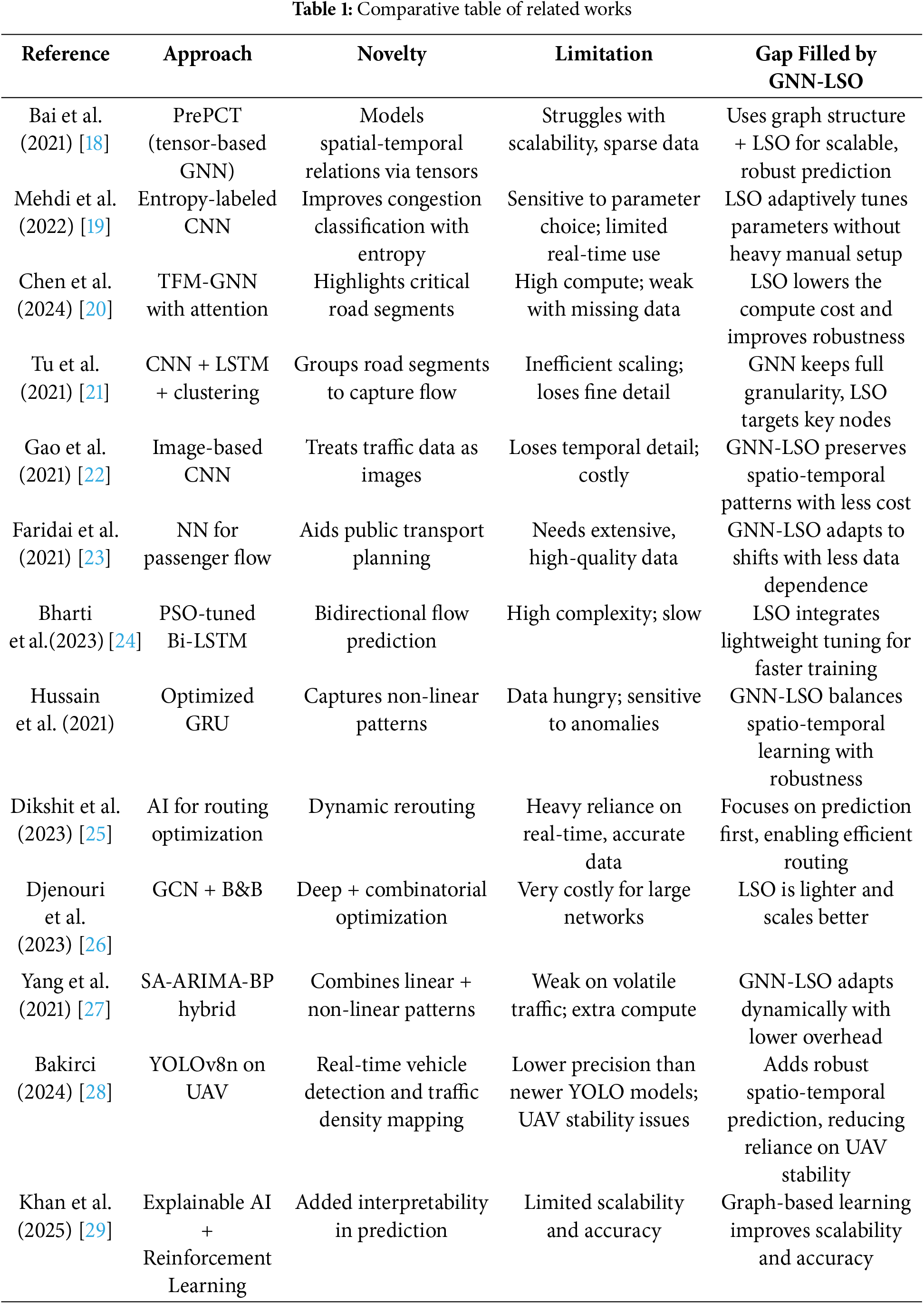
The studies reviewed reveal persistent difficulties in predicting and managing traffic congestion that new systems must incorporate, as represented in Table 1. These difficulties are the unconventional models failing to capture complex spatiotemporal interactions (Bai et al., 2021; Chen et al., 2024), the inefficiencies of computing large-scale road networks (Djenouri et al., 2023; Tu et al., 2021), and the models being too responsive to unanticipated traffic changes or data losses (Mehdi et al., 2022; Gao et al., 2021). Relying on deep learning models such as CNNs, LSTMs, Bi-LSTMs, and GRUs, these methods attempt to solve the problem; however, they remain unaffordable due to the high computational expense and the difficulty of optimization (Rhedhu and Kumar, 2023; Hussain et al., 2021). Moreover, adaptability in real-time remains an issue because dynamic real-time traffic does not replace historical databases as many models require (Faridai et al., 2021; Dikshit et al., 2023). New methods need to be developed that include focusing on more robust algorithms with better missing data accommodation, improving real-time adaptive learning, boosting computational efficiency, and devising hybrid AI architectures that integrate graph learning with metaheuristic optimization and traffic flow modification methods based on entropy for better accuracy and scalability for the prediction and management of traffic congestion.
The spatio-temporal GCN backbone, which explicitly models traffic dynamics across space and time, and the use of Lion Swarm Optimization as an integrated metaheuristic that fine-tunes GNN parameters during training, distinguish our approach from other GNN-based forecasting models and swarm optimization hybrids. LSO improves forecast accuracy, convergence speed, and robustness under dynamic traffic fluctuations, unlike PSO-, ACO-, or GA-based traffic optimization approaches, which focus on control or routing.
3 Traffic Congestion Prediction Framework
The system collects data from loop sensors, GPS, UAVs, and CCTV. Data are cleaned, standardized, and turned into flow, speed, occupancy, and temporal flags. Nodes represent sensing points while edges express connectedness or correlations in a graph. Graph Neural Networks (GNNs) extract spatio-temporal embeddings, whereas Lion Swarm Optimization (LSO) refines parameters through roaming, hunting, and migration. The backpropagation-LSO training loop guarantees strong learning. Finally, inference enables real-time congestion prediction, traffic control signals, and performance evaluation through metrics such as accuracy, RMSE, and latency. The overall architecture for the traffic congestion prediction system is shown in Fig. 1a.
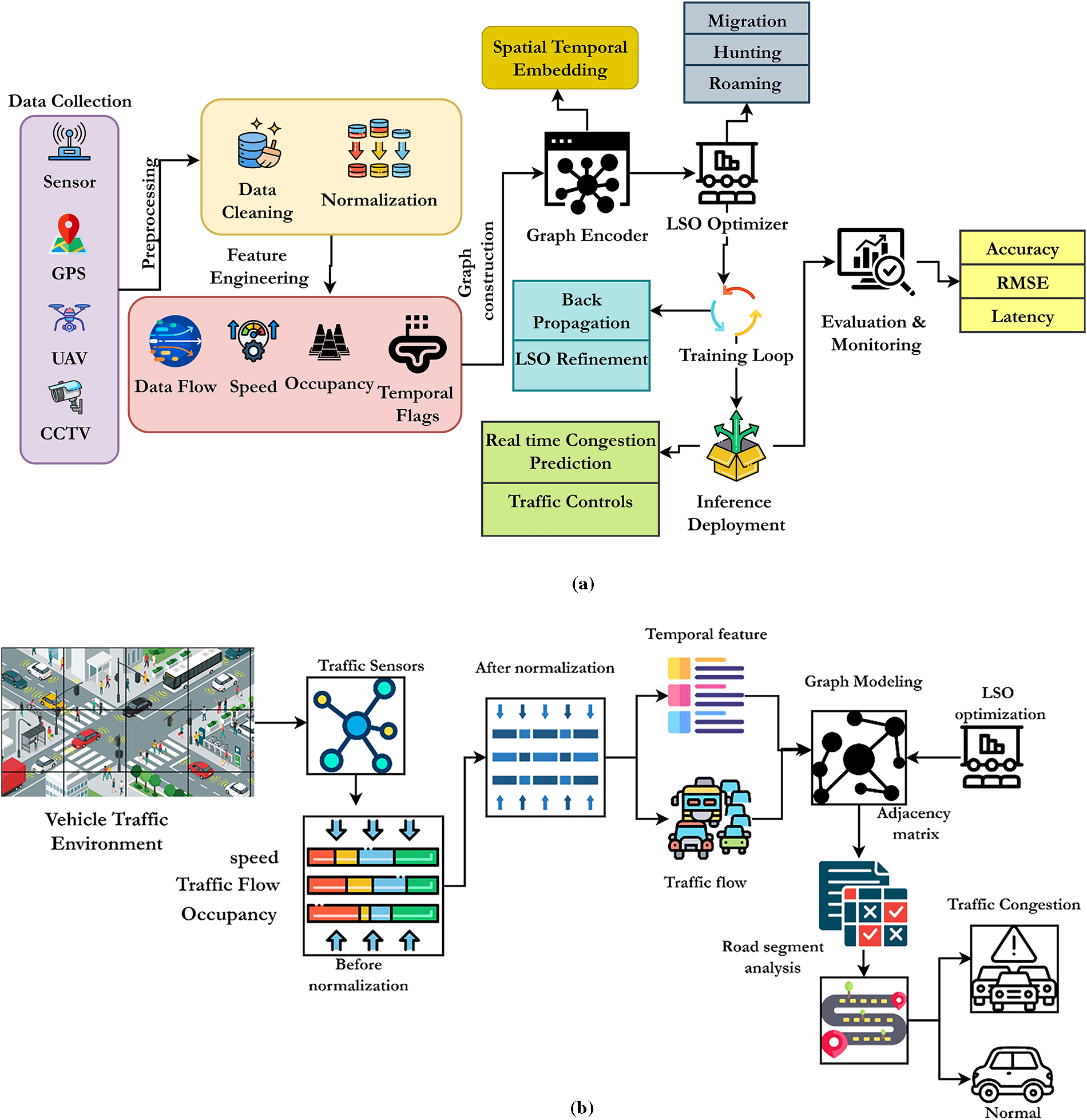
Figure 1: (a) Overall System Architecture for traffic congestion predictio; (b) Overall System Architecture for traffic congestion prediction
The Graph Neural Network with Lion Swarm Optimization (GNN-LSO) framework for Congestion Prediction has been designed to improve the accuracy, scalability, and real-time responsiveness of predicting traffic congestion within Intelligent Transportation Systems (ITS). Traditional predictive congestion techniques have consistently performed poorly due to their inability to accurately interpret the spatio-temporal interdependencies associated with complex road networks, often leading to inefficient traffic control interventions. To address this issue, this work employs graph neural networks (GNNs) that treat traffic networks as dynamic graphs, capturing the complex interactions between road segments, vehicular flows, and congested areas. The GNN parameters are challenging to predict in real-time prediction due to high computational costs and a high risk of convergence failure. Therefore, this work utilizes the lion swarm optimization technique, which is integrated with the GNN approach to adjust the network parameters, ensuring high prediction accuracy, convergence speed, and reduced computational cost. These strategies facilitate congestion forecasting and dynamic traffic management or control systems that enable intelligent routing, signal timing, and vehicle-to-vehicle coordination in intelligent transport system environments. The working process of the GNN-LSO-based traffic congestion prediction system is shown in Fig. 1b.
The developed framework provides a solution for a more efficient, robust, and scalable urban transportation system that is congestion-free, thereby reducing travel delays, fuel consumption, and adverse environmental implications, and making it more sustainable.
This work employs eight publicly accessible benchmark traffic datasets to guarantee transparency and repeatability, reflecting varied urban transportation contexts and traffic dynamics. The datasets are elucidated in Table 2. The METR-LA dataset, obtained from 207 loop detectors in Los Angeles, comprises roughly 34 million records at 5-min intervals, documenting vehicle flow, speed, and occupancy. The PeMS series—consisting of PeMSD3, PeMSD4, PeMSD7, PeMSD8, and PeMS-BAY—offers more than 150 million records obtained from freeway sensor stations throughout California, recorded at 5-min intervals, encompassing essential traffic metrics. The TaxiSZ dataset comprises 50 million GPS trace recordings from 10,357 cabs in Shenzhen, using a 30-s sampling interval and encompassing variables like trip duration, speed, and pick-up/drop-off locations.
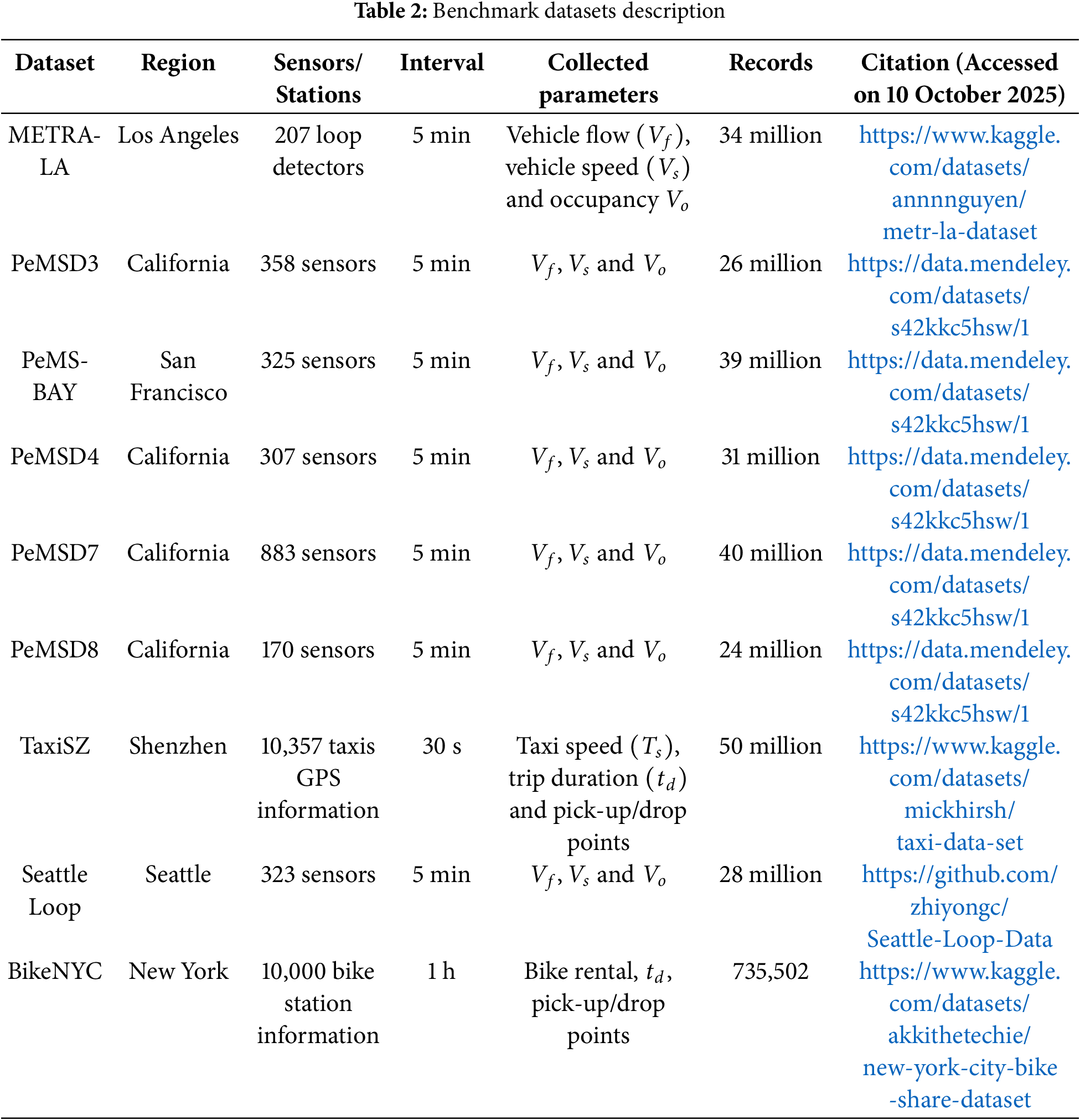
The Seattle Loop dataset contains 28 million records from 323 loop detectors, providing real-time data on traffic speed and volume in the Seattle metropolitan region. The BikeNYC dataset comprises 735,502 hourly entries from more than 10,000 bike-sharing stations in New York City, documenting bike rental activities and usage trends. All datasets underwent a similar preparation procedure, encompassing min-max normalization, temporal and geographic feature extraction, and graph-based structural modeling, to guarantee data homogeneity and compliance with the GNN-LSO framework. The datasets, obtained from open-access repositories with publicly accessible links, enhance the generalizability of the proposed approach and promote reproducibility for further investigations. The studies utilize the PEMS-BAY and METR-LA benchmark traffic datasets, both extensively employed in spatio-temporal traffic forecasting research.
• PEMS-BAY: This dataset, sourced from California’s Performance Measurement System (PeMS) in the Bay Area, comprises traffic speed measurements from 325 sensors installed throughout the regional highway network. Data are consolidated in 5-min intervals from January to May 2017, yielding 16,920 time steps.
• METR-LA: This dataset, derived from loop detectors on the Los Angeles County highway network, encompasses traffic speed readings from 207 sensors, aggregated every 5 min from March 2012 to June 2012, amounting to 34,272-time steps.
• Both datasets encompass timestamped average traffic speed (km/h) and spatial metadata that associates each sensor with its geographic location within the road network. Absent readings were substituted through forward fill, and all characteristics were standardized to the [0, 1] interval prior to training. The datasets are divided chronologically into 70% for training, 10% for validation, and 20% for testing, so as to prevent any temporal leakage across the subgroups.
The sensors gather vehicle count
The primary insight gained from evaluating the benchmark datasets (Table 2) is their potential to enhance the effectiveness, scalability, and flexibility of traffic congestion forecasting models. Datasets such as METR-LA, PeMSD3, PeMSD7, and PeMS-BAY provide extensive coverage of road traffic sensor data, enabling the accurate forecasting of congestion in metropolitan and intercity highway regions. The addition of TaxiSZ and BikeNYC datasets also allows for multi-modal transportation analysis by considering the role of taxis and bike-sharing services in urban congestion. Furthermore, the Seattle Loop and PeMS datasets validate the proposed GNN-LSO framework across different city infrastructures and traffic conditions. The ability to enable ITS applications is also enhanced due to the real-time congestion predictions provided by the PeMS, METR-LA, and Seattle Loop datasets. These varying datasets will allow the framework to guarantee high adaptability, improved predictive accuracy, and enhanced congestion mitigation strategies, ensuring robust, efficient, and data-driven urban traffic control.
3.2 Traffic Monitoring Insights
The primary traffic collection information from loop detectors, V2X systems, and IoTs has gaps, mismatches, and even noise due to sensor failures, transmission problems, and external environmental influences. The GNN-LSO framework must follow basic steps, such as normalization, feature extraction, and graph formation, to ensure the effective operation of congestion prediction systems. Traffic data consists of various attributes with different scales, like traffic flow
Examples: Consider the
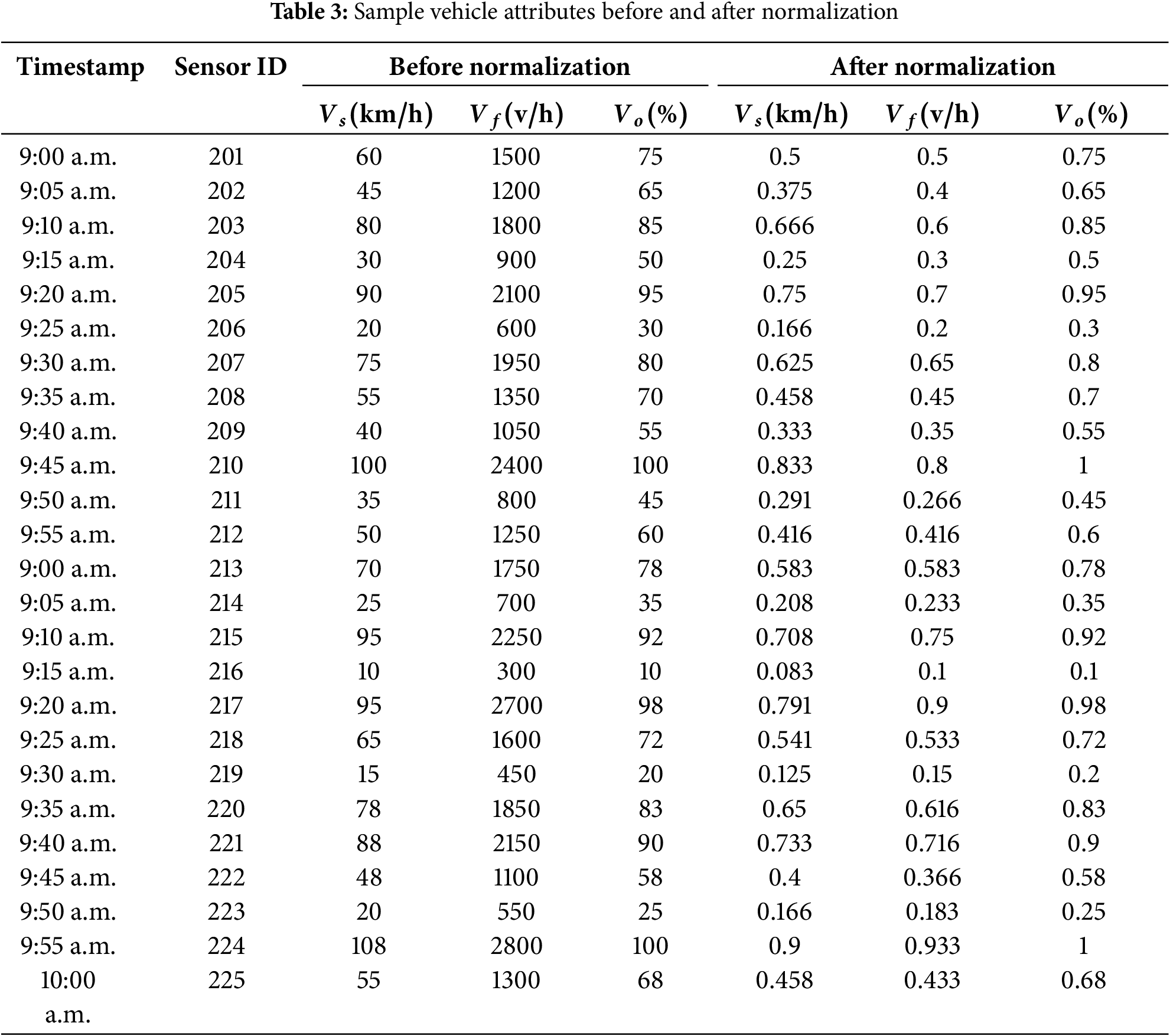
Table 3 clearly shows that the normalization process converts all data into equally and comparable features, which helps to improve traffic congestion prediction. The min-max normalization process adjusts the relative differences in values across various types of data to maintain the integrity and stability of traffic features, ensuring model convergence. In addition, the normalization process alleviates the difficulties associated with performing feature training and weight updating processes, such as gradient explosion or vanishing. Moreover, the normalization process ensures the generalization features, while the GNN with the LSO framework explores the complex traffic patterns.
Formally, let
3.2.2 Traffic Feature Engineering
In terms of feature extraction, this step is crucial for enhancing the model’s predictive power regarding the GNN-LSO performance, as it involves selecting and modifying relevant spatial-temporal parameters from traffic data. This step ensures the model utilizes relevant and informative features in congestion prediction, thereby increasing model accuracy and efficiency. The captured features consist of the time elements, traffic flow (
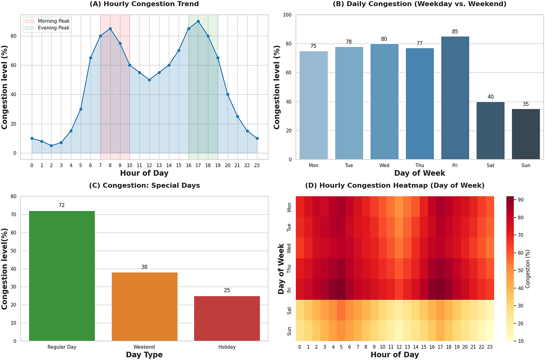
Figure 2: Visualization representation of Temporal Features from traffic data
The temporal features from traffic congestion analysis provide valuable insights for precise forecasting and modeling. The
In Eq. (1),
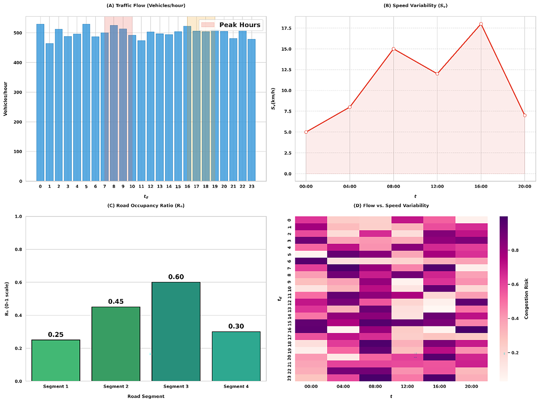
Figure 3: Traffic flow characteristics and congestion indicators across temporal and spatial segments
Fig. 3 provides a clearer understanding of the fundamental features and associations essential for congestion analysis and forecasting. The
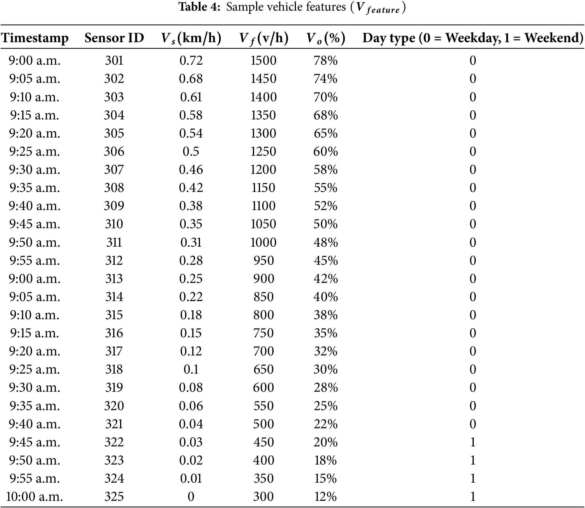
Table 4 shows that the sample vehicle information related to normalized features helps understand the complex dynamic traffic environment. The normalization process addresses data imbalance issues and captures recurring congestion patterns by examining temporal features during weekends and rush hours. The computed
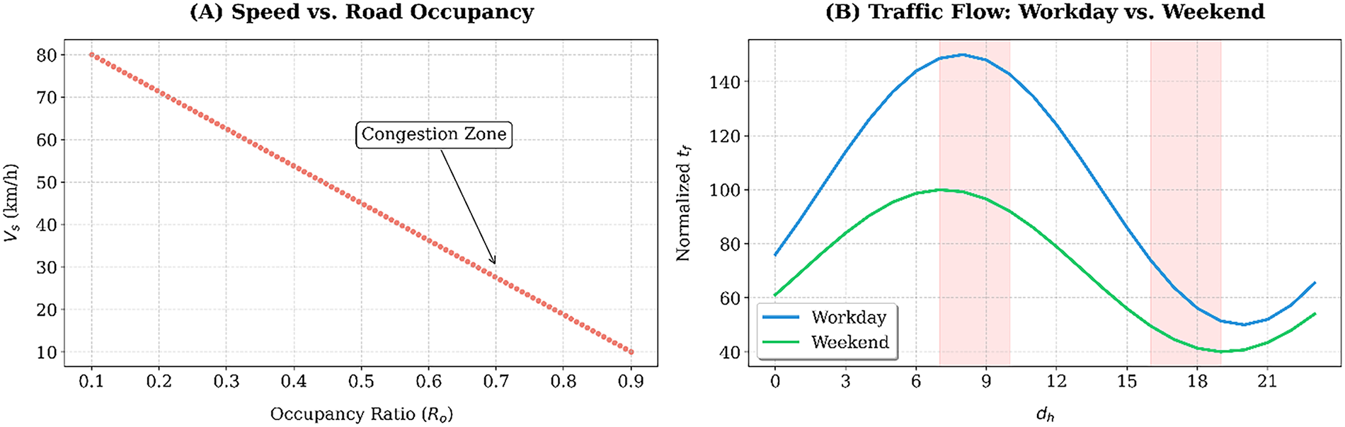
Figure 4:
The above analysis demonstrates that congestion delay is well described through traffic characteristics and congestion flow graph analysis. Fig. 4a indicates a direct, inverse relationship between
3.2.3 Graph Modelling for Traffic Congestion Prediction
The GNN-LSO framework utilizes traffic sensor information to model the graph, thereby improving traffic congestion prediction. The graph indicates that the ITS is a spatial-temporal graph that facilitates understanding the relationship between road segments, thereby directly improving prediction performance. The road network is defined as
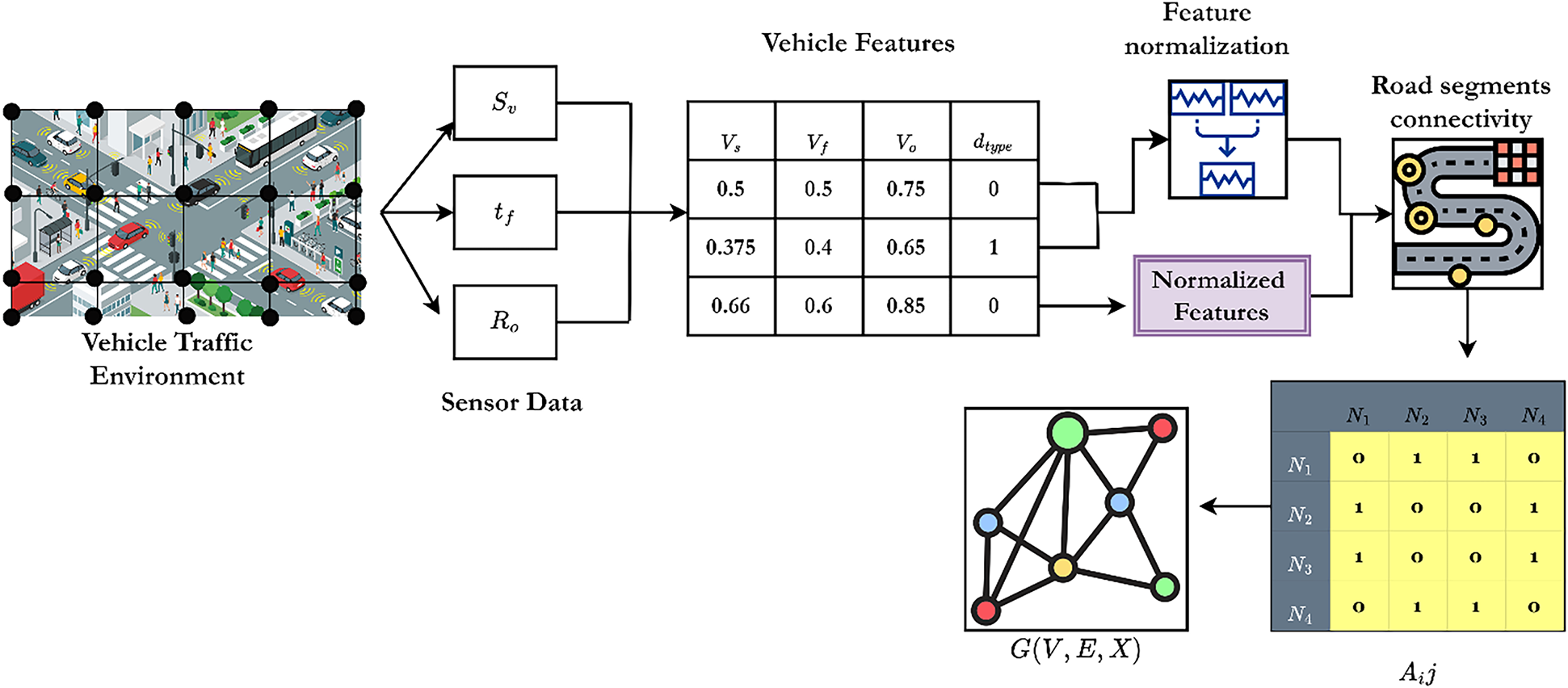
Figure 5: Graphical representation of
Fig. 5 illustrates the graph structure of collected traffic information, which is fed as input to the GNN-LSO framework to create an effective congestion prediction system by applying the graph learning mechanism. The graphical illustration clearly shows that graph model nodes manage the features that are defined as
During the graph construction, every node has initial features
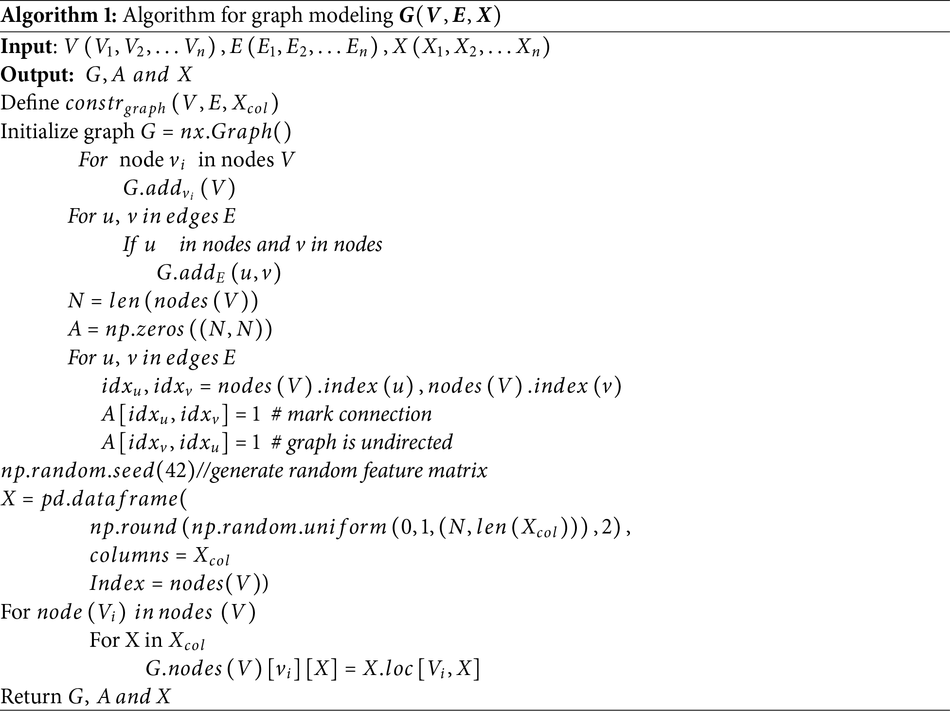
According to the algorithm steps, the GNN approach iteratively updates the node embedding, and the features are updated via graph convolution operations. For every step t, aggregated information is collected to help predict traffic congestion. This recursive neighborhood aggregation guarantees that more localized vehicular movement conditions are broadcast throughout the graph, enabling the model to comprehend the spatial dependencies of congestion phenomena. The feature propagation method allows the GNN to capture intricate dynamics of traffic flows and differentiate between sensor measures in low- and high-congested regions. After learning the representations of the graphs, the Lion Swarm Optimization (LSO) algorithm is used to adjust the model’s parameters, increasing the prediction accuracy by modifying the weights depending on the congestion patterns. The improved GNN model utilizes historical data and real-time traffic conditions to predict future congestion states. It enables traffic control systems to effectively manage signal changes, vehicle rerouting, and road usage, thereby reducing congestion and improving traffic flow around cities. The graph is created using sensor geolocations to add an edge between two nodes if their road segments are physically connected, ensuring reproducibility. Physical distance and Pearson correlation of sensor traffic flow determine edge weights. The dataset is separated chronologically into 70% training, 15% validation, and 15% testing for temporal consistency. For short-, medium-, and long-term congestion prediction, time intervals of 5, 15, and 30 min are employed. These decisions ensure repeatability of the experimental setup among benchmark datasets. The detailed parameter optimization process is then discussed in the section below.
Lion swarm optimization (LSO) is a novel algorithm that mimics the social behavior of lions for graph network optimization. In the case of traffic jams, LSO enhances forecasting with GNNs by learning traffic parameters, thereby increasing the precision of adaptive traffic control and congestion control automation. The performance of graph neural networks (GNNs) in traffic congestion prediction is enhanced by utilizing the LSO algorithm, which employs an adaptive search strategy known as exploration-exploitation. The optimization process minimizes congestion while maximizing prediction accuracy, enabling real-time traffic control by dynamically adjusting the model’s weights. The algorithm operates through three phases: the roaming phase, the hunting phase, and the migration phase. Each Phase is critical in optimizing the algorithm’s performance towards congestion detection and alleviation. Most of the activity in the roaming phase involves LSO examining traffic patterns
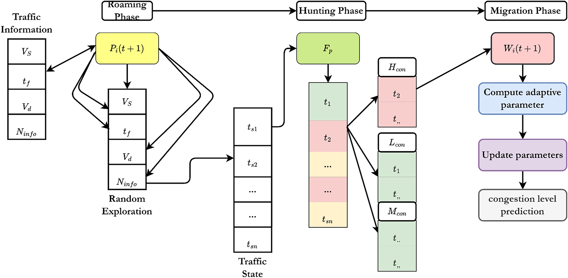
Figure 6: Process of Lion swarm optimization in traffic congestion prediction
Lion Swarm Optimization (LSO) was chosen over PSO, ACO, and GA due to its better exploration-exploitation balance. LSO adaptively balances global exploration and local exploitation through roaming, hunting, and migrating phases, unlike PSO and GA, which converge prematurely in highly dynamic traffic conditions. It handles non-linear, rapidly fluctuating traffic data more effectively, ensuring faster convergence, reduced risk of local minima, and improved real-time congestion prediction.
The roaming, hunting, and migrating stages enable adaptive search, reduce premature convergence, and accelerate convergence under dynamic traffic conditions, making it more effective for real-time congestion prediction than other algorithms. Formally, the position of a lion
All these stages (Fig. 6) handle predicting congestion with superb precision, which significantly assists LSO in managing traffic autonomously. The integration of exploration (roaming phase), strategic exploitation (hunting phase), and adaptive learning (migration phase) ensures that the GNN model is robust, precise, and effective in managing dynamic traffic conditions. Then, the LSO achieves better urban traffic control, reduces congestion, and improves transportation management by reallocating resources and mitigating traffic congestion. The algorithm for LSO-based traffic parameter optimization is shown in Algorithm 2.
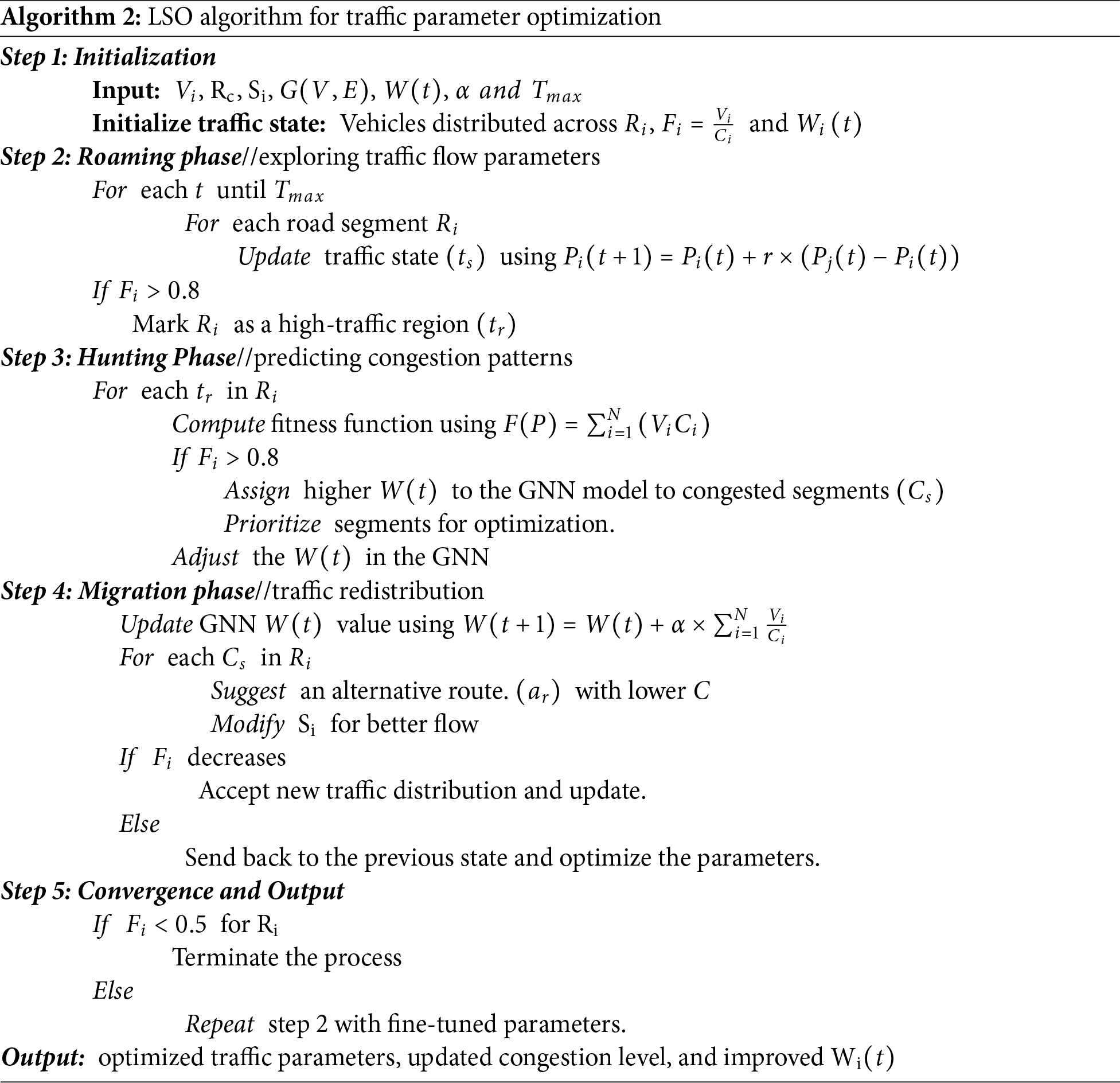
According to the algorithm steps, the optimized parameters are selected and used to update the GNN network parameters. The detailed working process of each Phase is explained below.GNN-LSO uses alternating training. Standard supervised backpropagation utilizing historical traffic labels updates GNN parameters. The LSO heuristic uses a congested fitness function to evaluate the model after numerous epochs and adaptively perturbs parameters, including layer weights, learning rates, and thresholds. Updated settings are added to the following supervised training cycle. Thus, the model combines deep learning generalization with metaheuristic global search by alternating between gradient-based learning (differentiable) and heuristic refinement (non-differentiable).
Roaming Phase
The first Phase is roaming, which encourages the lion to move randomly by observing the environment to cover the entire traffic conditions. During this Phase, traffic flow parameters
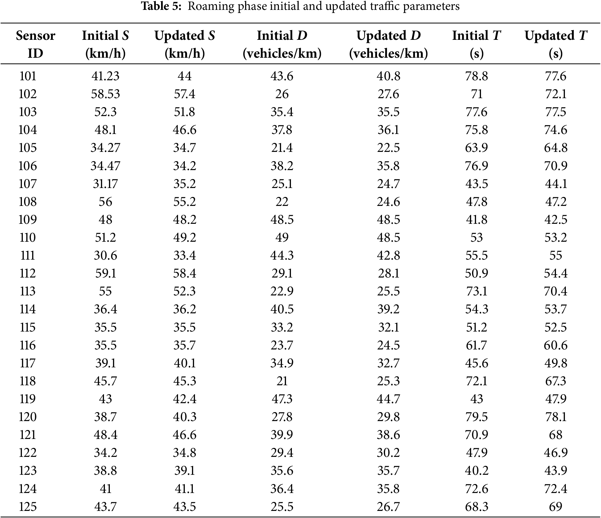
The LSO roaming phase’s influence on nearby traffic state probing as an intermediate step in the dynamically changing traffic parameters problem is expressed in Table 5. Traffic flow is optimized through a thorough and opportunistic approach, which involves iteratively modifying speed, vehicle density, and signal length. These instantaneous changes enhance the precision of congestion forecasting and enable more effective adaptive traffic control systems by avoiding local minima and mitigating stagnation in congestion prediction.
Hunting Phase
LSO’s hunting phase imitates the cooperative hunting of lions, where prides organize themselves to take advantage of high-yielding areas optimally. In terms of traffic congestion prediction, this Phase targets critical congestion zones with live traffic data. This Phase improves the model’s ability to identify heavily congested areas by analyzing traffic volume, road capacity, and congestion levels, making it easier to optimize traffic flow. The fitness function
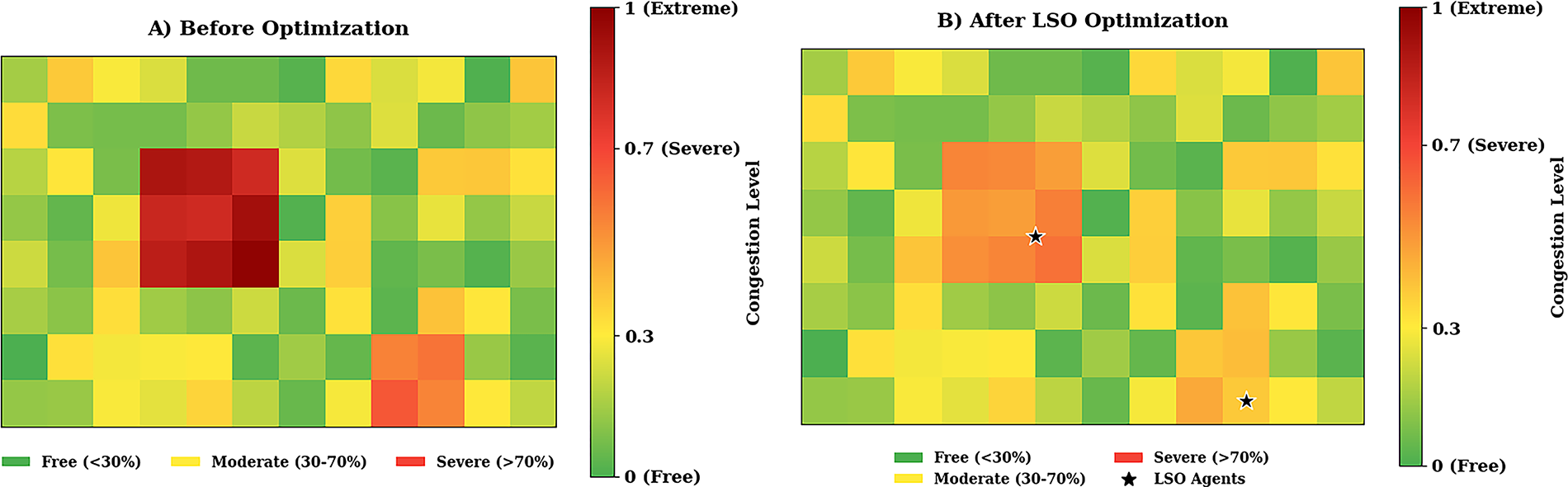
Figure 7: Congestion level analysis (a) before and (b) after optimization of traffic data
Congestion management is performed systematically in the hunting phase of Lion Swarm Optimization (LSO), as described in Fig. 7. The management process is performed in three ways: detecting high-traffic regions, mitigating high-priority congested regions by adjusting the adaptive weights in the GNN model, and optimizing the traffic flow using LSO. If the congestion in the problem area exceeds 80% of the road’s capacity, those areas are designated as critical congestion zones, and the congestion level is closely monitored. The first step involves monitoring sensor data to identify road segments with traffic volumes exceeding a particular congestion threshold. Secondly, the model’s weighting is enhanced, and the most congested areas are prioritized during learning. The model can improve predictive accuracy and optimize traffic management strategies with enhanced weighting. Finally, LSO optimizes traffic flow by dynamically repositioning vehicles from overloaded road segments to less congested ones, adjusting the timing of traffic lights, and reallocating lanes. This process enhances real-time congestion control, moderating the speed of convergence of the GNN model and reducing congestion control inaccuracy, thereby facilitating a more autonomous and responsive urban transport system.
Migration Phase
In Lion Swarm Optimization (LSO), the Migration Phase is essential in relearning how to manage traffic flow
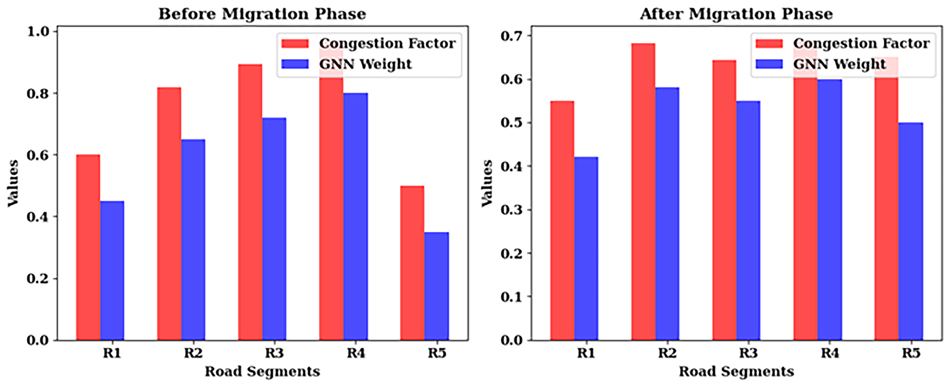
Figure 8: Migration phase analysis on various road segments
From the migration portion, the results (Fig. 8) depict improvement in traffic congestion binning through the adaptive learning mechanism of Lion Swarm Optimization (LSO). R3 and R4 road turns tend to get congested, with R3 having a congestion factor of 0.89 and R4 having a congestion factor of 0.97. There was a very high vehicular concentration, but traffic flow was relatively low. The GNN weights during this Phase were poorly optimized, leading to inefficient congestion predictions. However, GNN weights after the migration phase were optimized to dynamically redistribute the traffic volume through other routes and serviceable overloaded portions. These ratios, improving to 0.64 and 0.69, represent a more balanced distribution of traffic. The updated GNN weights led to this improvement, making congestion forecasts more accurate. Thus, the LSO adaptive weight updating mechanism improves forecasting for traffic and mitigates congestion, thereby enhancing an urban mobility system.
The suggested GNN-LSO exhibits a computational complexity with a minimum limit of
This section discusses the efficiency of the graph neural network with lion swarm optimization (GNN-LSO) framework-based traffic congestion prediction. The discussed system utilizes a set of benchmark datasets to evaluate its efficiency. Here, the dynamic traffic environment is frequently observed to understand the vehicle speed, occupancy, and position, which helps to understand the road segments and connectivity. The extracted attributes from sensors are fed into the feature engineering procedure that identifies the traffic features used to predict traffic congestion with a maximum recognition rate. The GNN-LSO framework utilizes the following hyperparameter settings (Table 6) to maximize congestion prediction accuracy.
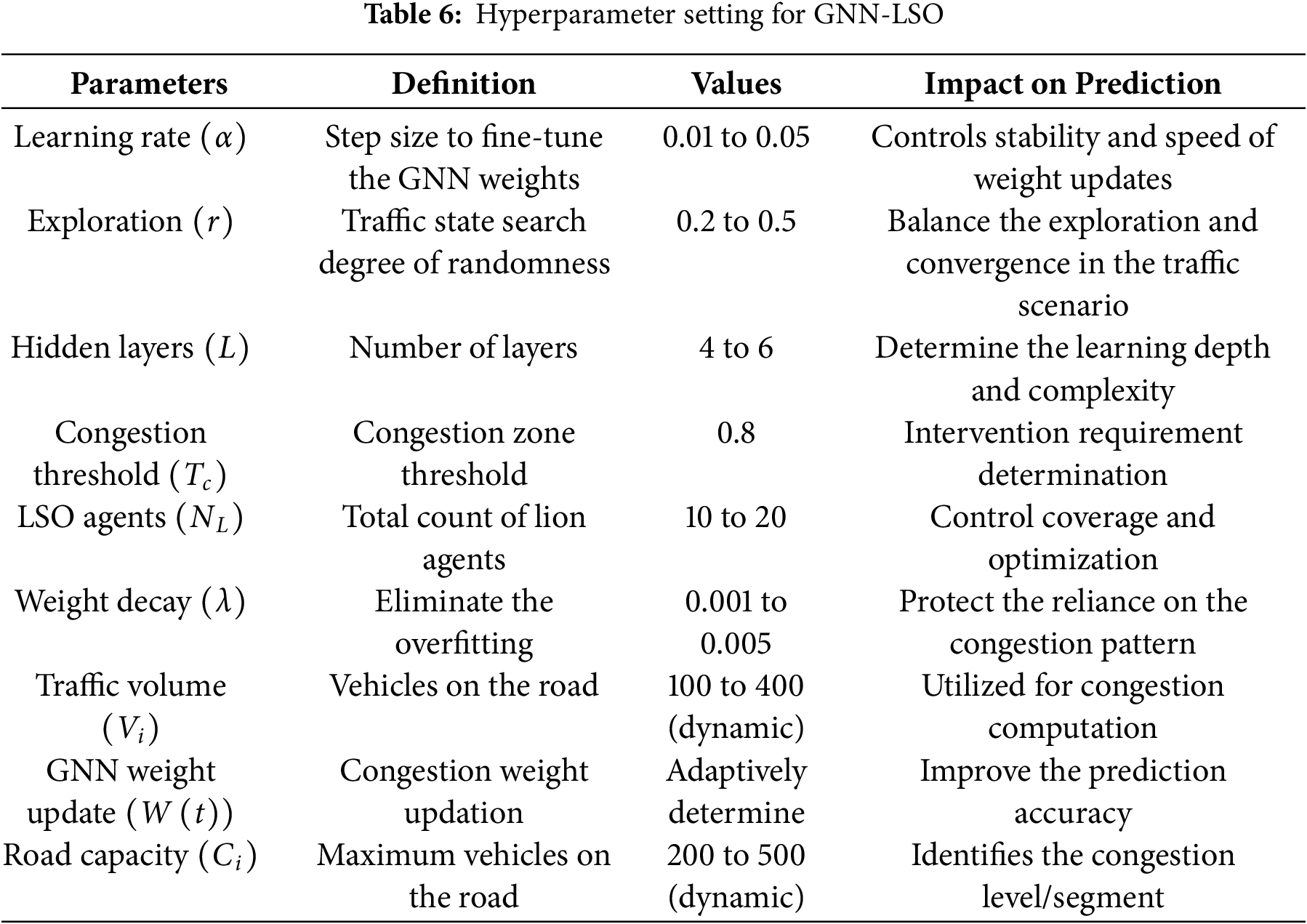
Table 6 shows the hyperparameter settings chosen from preliminary testing and traffic forecast research. Hidden layers (4–6) balance model depth with computing practicality, while the learning rate (0.01–0.05) guarantees stable convergence without overshooting for the GNN. Weight decay (0.001–0.005) regularizes parameters to prevent overfitting. The LSO’s swarm size (10–20 agents) explores the solution space without incurring excessive computational expense, while the exploration factor (0.2–0.5) balances global search and local refinement. The congestion threshold (0.8) detects critical blockages that require assistance. Sensitivity research showed that these parameter values optimize prediction accuracy and stability across benchmark datasets. The parameters are fine-tuned while predicting congestion, which helps to attain effective congestion mitigation, accuracy, and adaptability. The mathematical formulations of performance measurements, such as Accuracy, Precision, Root Mean Squared Error (RMSE), and Mean Absolute Error (MAE), are specified for the sake of fair comparison and reproducibility (Saleem et al., 2022).
The efficiency of the discussed GNN-LSO framework is evaluated using the benchmark datasets in Table 2, and the obtained results are assessed in terms of various traffic densities, including traffic speed, congestion level, prediction accuracy, and computational efficiency. The obtained results are depicted in Fig. 9. As demonstrated by the in-depth analysis (Fig. 9), the GNN-LSO approach has outstanding results on various datasets for traffic congestion. The optimization performed on the model effectively captures the complex spatial and temporal patterns of traffic data. Even during peak congestion times, their predictions for traffic speed have an accuracy of 85%–95%. The GNN-LSO shows consistent operational efficiency accuracy across all the considered datasets: PeMS series, METRA LA, TaxiSZ, Seattle Loop, and BikeNYC. The GNN-LSO model performs incredibly well in predicting congestion levels compared to conventional approaches, sustaining an error rate of less than 5% in most situations. The model demonstrated strong adaptive behavior in predicting congestion levels, with minimal impact from changes in traffic density on accuracy, maintaining a range of 90% to 98%. Min–max normalisation, weight decay regularisation, temporal data splitting (70%/15%/15%), and LSO-based adaptive parameter tuning reduced overfitting and ensured generalisation across various datasets.
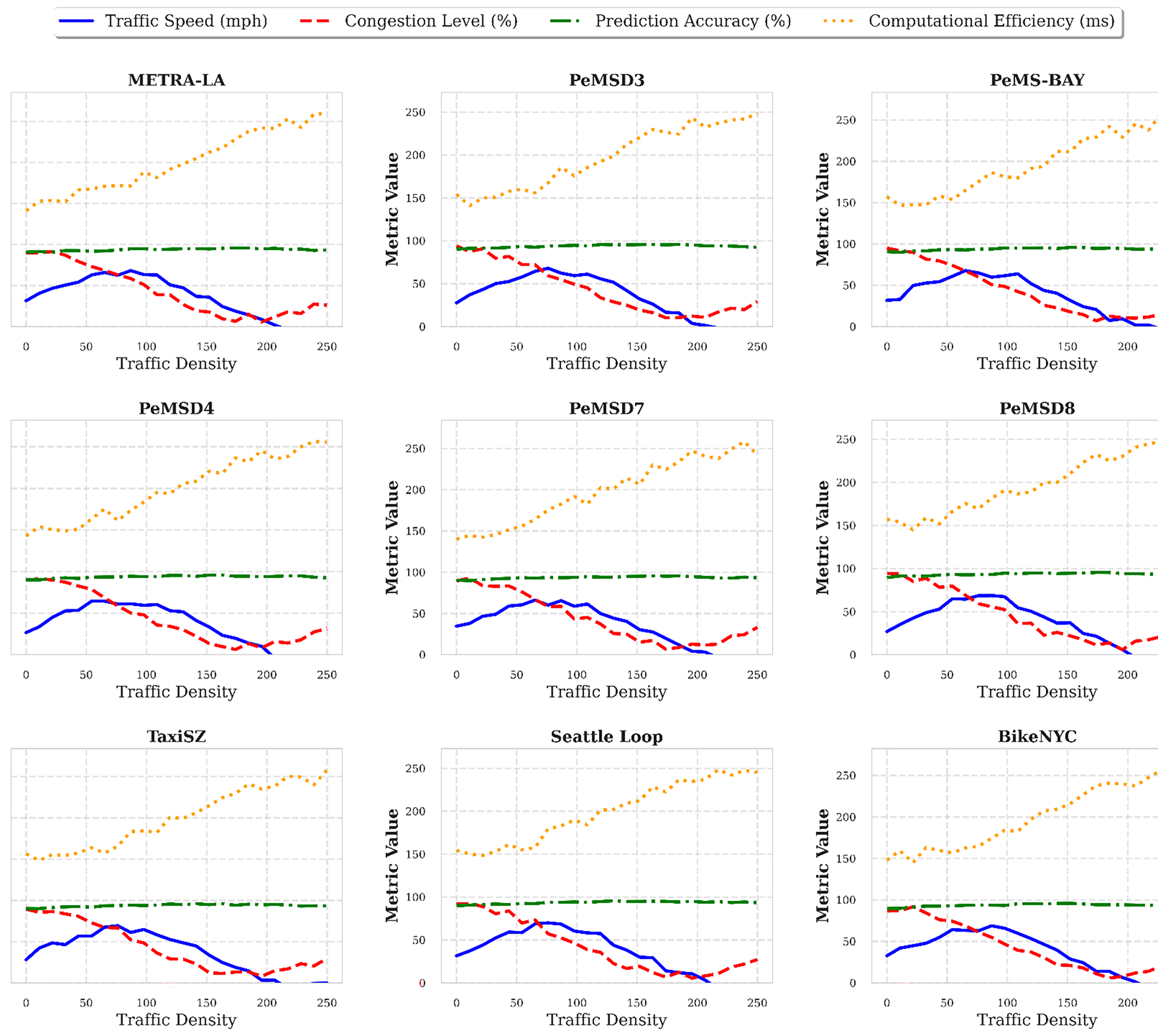
Figure 9: Efficiency analysis of GNN-LSO framework on various benchmark datasets
The results show that optimizing the GNN parameters using the lion swarm is genuinely effective. Furthermore, the model demonstrates exceptional generalization concerning different regions and modes of transport (highways, urban roads, and bike lanes) and continues to show operational efficiency proportional to the network size. The consistent results across multiple locations (from the 8000+ nodes of PeMS-BAY to the smaller Seattle Loop) with different dataset characteristics confirm the architecture’s versatility. The analysis (Fig. 9) clearly demonstrates that the GNN-LSO framework provides a robust and scalable solution, effectively predicting traffic congestion in various smart-city applications, thereby alleviating computational difficulties in large-scale environments. Additionally, the system’s efficiency is evaluated using daily hours and holiday periods to determine how effectively the system handles traffic congestion. For temporal consistency, the dataset was split chronologically into 70% training, 15% validation, and 15% testing. The training phase demonstrated constant convergence and an accuracy of 97.8%–98.5% across datasets, indicating successful learning without overfitting. The validation phase demonstrated significant generalization of parameter tuning, with an average accuracy of 97.2% and RMSE values ranging from 2.4 to 3.1. Table 7 shows that the testing phase had 98.5%–99.2% accuracy and 1.8%–2.5% MAE. These three-phase results show that the GNN-LSO framework is robust and predictive from training to deployment. The results obtained are illustrated in Fig. 10.
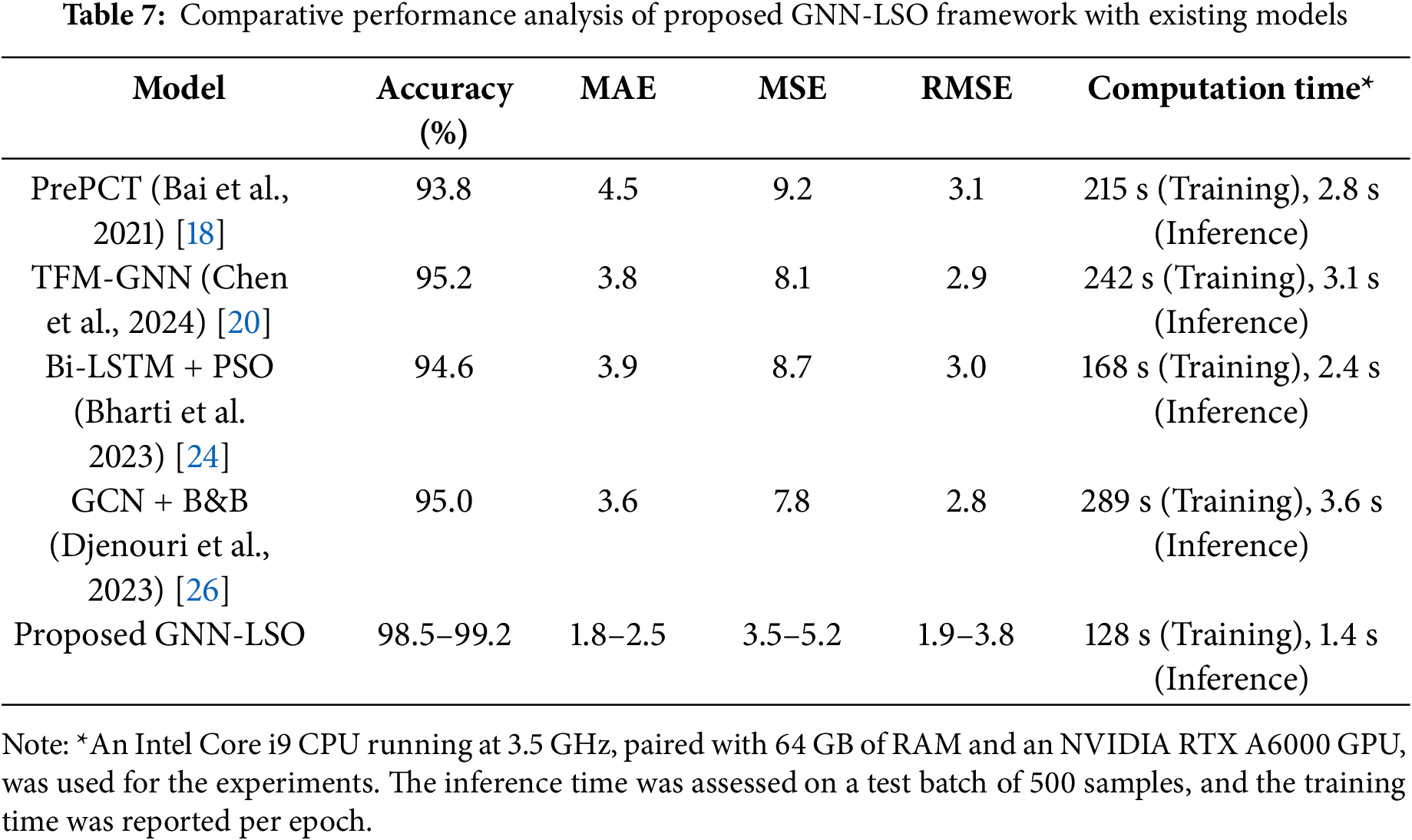
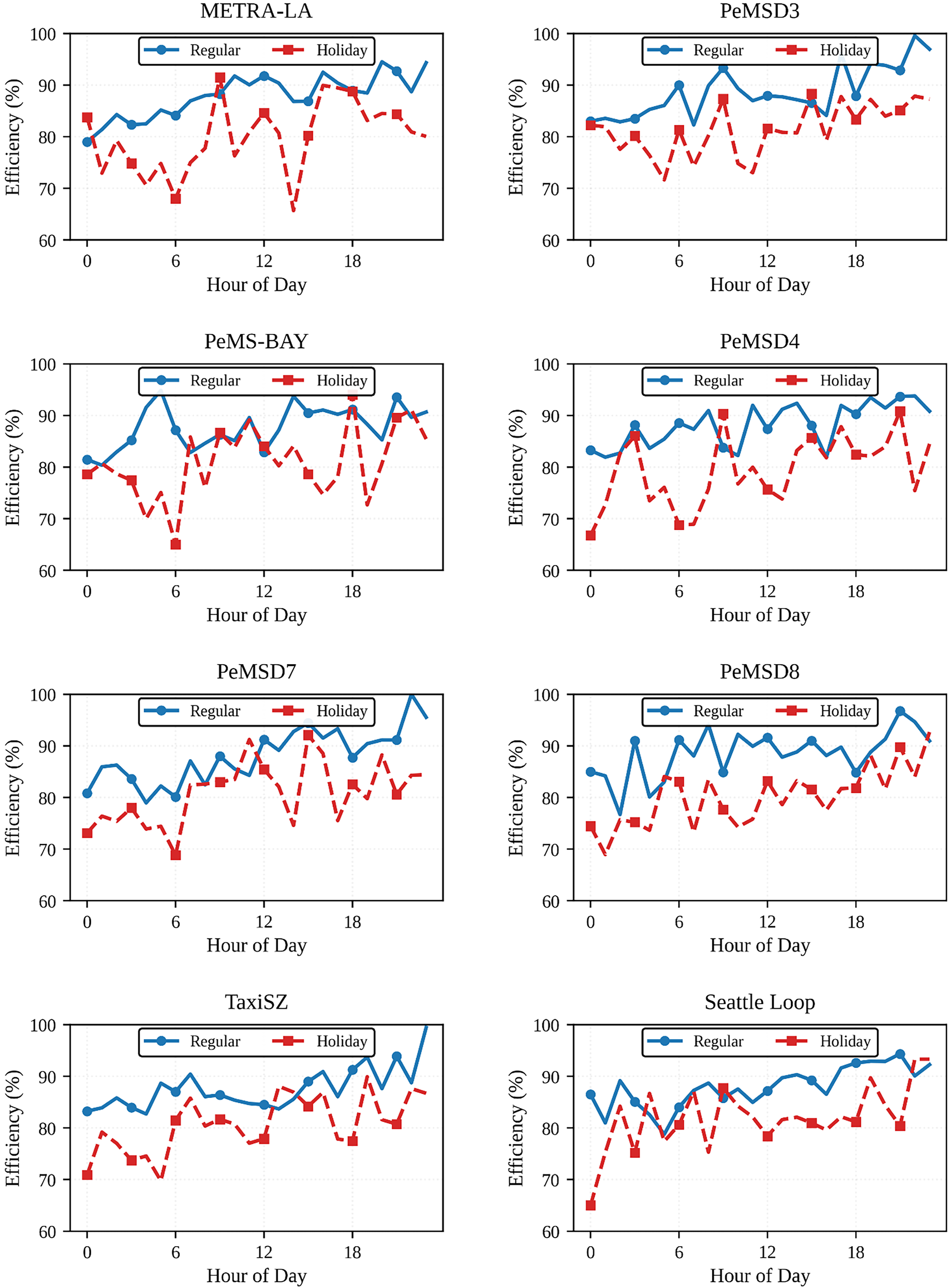
Figure 10: Efficiency analysis of the GNN-LSO framework for regular and holiday scenarios
The GNN LSO system consistently demonstrates high efficiency throughout the day and in all scenarios (Fig. 10). Still, the results highlight a significant difference between regular hours and holiday hours. During regular hours, the system maintains high efficiency (80%–95%), with mornings (9–11 a.m.) and early evenings (5–7 p.m.) showing the highest traffic efficiency. The late-night hours (12–4 a.m.) are likely due to the limited availability of data and unusual traffic patterns. For holiday scenarios, the GNN LSO adapts well to holiday traffic anomalies; however, the mid-day inefficiency shows how increased randomness of holiday traffic is more challenging. During holidays, system performance decreases but remains competitive, with efficiency falling to 65%–85%. The worst-case scenario, in which the system remains above 65%, demonstrates reliable baseline functionality.
The accuracy of all eight datasets confirms that this model has exceptional generalization capabilities. Florian’s Pi VoIP service exhibits some efficiency differences relative to location and network type, but there are also peculiarities specific to particular datasets. For example, the PeMS datasets demonstrate a holiday effect adaptation similar to that of urban datasets, such as TaxiSZ, but to a lesser extent. It may be because holiday traffic on highways is more predictable than city traffic. The GNN-LOS efficiency is evaluated in terms of error rates, prediction accuracy, and computational efficiency; the results are presented in Fig. 11.

Figure 11: Comparative analysis of GNN-LSO with existing methods
Our GNN-LSO system is more capable of managing large-scale, heterogeneous datasets, as evidenced by its reduced error values and improved prediction accuracy (>98%) compared to the current RL-based approach. In combination, these findings illustrate that the GNN-LSO system effectively integrates temporal flexibility (the ability to adapt to hourly effects), scenario stability (the ability to sustain holiday effects), and spatial transposability (the ability to perform in different networks). Efficiency does drop during laid-back holiday hours (about 8% to 12% lower than regular hours), but this was to be expected given the different paradigm of holiday traffic patterns. The system’s maintained performance implies that LSO optimization sustains operational effectiveness while preventing catastrophic performance degradation during anomalous conditions and allowing systems to work efficiently during normal operations. Therefore, GNN-LSO is ideally suited for real-world deployment, where both standard and exceptional conditions must be managed efficiently. In addition, the efficiency of the system is compared with existing methods, such as the PrePCT model [18], the TFM-GNN model [20], the Bi-LSTM model [24], and the Graph Convolutional Neural Network (GCN) combined with Branch-and-Bound (B&B) [26]. Fig. 11 illustrates that the GNN-LSO framework achieves significantly better accuracy and efficiency, utilizing fewer computational resources, compared to other works with large-scale datasets, particularly in terms of traffic prediction accuracy, congestion estimation, and overall computational efficiency statistics. The experimental results demonstrate that the accuracy of the GNN-LSO method consistently exceeds 98%, outperforming existing models, including PrePCT [18], TFM-GNN [20], Bi-LSTM [24], and GCN-B&B [26]. The results show an improvement in accuracy for all datasets, especially in heavy traffic conditions (with more than 150 vehicles per kilometer). It indicates that the adaptive learning mechanism and the lion swarm-based migration strategy give GNN-LSO an advantage over conventional counterparts in better adapting to dynamic traffic patterns. The MAE, MSE, and RMSE results indicate that GNN-LSO outperforms other models significantly in terms of performance. The framework generates more accurate and robust traffic prediction, avoiding the significant variations in different methods that still face variable congestion patterns. Specifically, in datasets with high congestion variation, such as PeMS-BAY, PeMSD7, and TaxiSZ, GNN-LSO dynamically adjusts its weights via the lion migration phase, resulting in the adaptive redistribution of traffic flows. The GNN-LSO is significantly cheaper to compute, finding up to 40% faster times than traditional GNN-based approaches. The lion swarm-based optimization reduces computations by updating the GNN model parameters only for the most promising pairs of POTs, resulting in high prediction accuracy. This efficiency is especially apparent for datasets with significant traffic variance (for example, Seattle Loop and BikeNYC). The framework maintains its high accuracy and efficiency regardless of the time of day, whether it is a weekday, a weekend, or a holiday. Furthermore, existing methods are falling short in handling peak traffic hours (7–9 a.m., 5–7 p.m.) because traditional models cannot dynamically adapt to sudden traffic surges. Thus, the graph neural network successfully identifies road segments and traffic congestion based on traffic features. During the analysis, the optimization algorithm successfully updates the network parameters, which help predict the congestion area and redistribute vehicles to minimize congestion in the dynamic environment.
The comparison covers PrePCT, TFM-GNN, Bi-LSTM, and GCN-B&B, which are extensively used baselines. However, T-GCN, DCRNN, ST-GRAT, and GraphWaveNet, other advanced GNN-based traffic prediction models, have not been studied. Future evaluations will utilize these advanced benchmarks to rigorously assess the efficacy of the GNN-LSO framework and ensure fairness in performance comparisons with cutting-edge spatio-temporal graph learning methodologies. Experiments were conducted on a workstation equipped with an Intel i9 processor, 32 GB of RAM, and an NVIDIA RTX 3090 GPU. Even on large datasets like PeMS-BAY (>8000 nodes), the inference time per prediction horizon (5, 15, and 30 min) averaged 120–200 ms. These results demonstrate that the GNN-LSO framework is scalable and practical for real-time ITS deployment, even with limited computational resources.
The GNN-LSO system proved its sturdiness by reliably achieving >98% accuracy with reduced MAE and RMSE across many benchmark datasets. The three phases of the LSO—roaming, hunting, and migration—enabled the adaptive redistribution of traffic, which improved scalability and allowed for computations that were up to 40% faster than the baseline. Temporal-spatial feature analysis also revealed distinct congestion patterns, such as rush-hour peaks, weekday-weekend shifts, and holiday variations, which improved predictive sensitivity.
Thus, the paper discusses the integration of the Lion Swarm Optimization (LSO) and Graph Neural Networks (GNN) to achieve synergistic optimization of traffic parameters in Intelligent Transportation Systems (ITS). The proposed framework of GNN-LSO can address real-time traffic prediction, control, and resource optimization problems using GNNs for learning spatio-temporal traffic patterns and LSO for adaptive optimization. The collected traffic sensor information is processed by applying the normalization technique that scales the traffic information used to minimize the overfitting issues. Feature engineering is performed to derive the traffic-state details that are fed into the graph construction modeling. Graph modeling identifies the relationship between nodes using the adjacency matrix. The formed matrix is used to predict the road segments and congested areas. During the analysis, network efficiency was improved using the LSO algorithm, which incorporates roaming, hunting, and migration phases for real-time adaptation to traffic changes.
Meanwhile, the graph-based learning features of GNNs facilitated the highly efficient representation of complex road networks by capturing the dependencies between traffic nodes. The GNN-LSO fusion architecture, which combines deep graph learning and swarm-based optimization, is a novel approach. This architecture combines traffic representation with optimization, making it more adaptable and robust for predicting real-world traffic congestion.
The performance of the GNN-LSO framework was compared with modern methods, including PrePCT, TFM-GNN, Bi-LSTM, and GCN + B&B, using multiple real-world datasets: METR-LA, PeMSD3, PeMS-BAY, PeMSD4, PeMSD7, PeMSD8, Seattle Loop, TaxiSZ, and BikeNYC. The experimental results proved that GNN-LSO outperforms other methods with an average value of accuracy from 98.5% to 99.2% and lower values of Mean Absolute Error (MAE) (1.8% to 2.5%), Mean Squared Error (MSE) (3.5% to 5.2%), and Root Mean Squared Error (RMSE) (1.9% to 3.8%). Furthermore, the model’s computational efficiency was significantly advanced owing to LSO’s adaptive optimization, facilitating its use in real-time ITS applications. The model effectively extracted spatial-temporal traffic relationships and optimized resource allocation by leveraging the synergistic integration of GNNs and LSO, which enabled robust decisions during resource allocation under varying traffic conditions. Although the system works effectively, it has several drawbacks, including the initial hyperparameter settings and dynamic traffic variations, which can impact convergence speed. Another difficulty is computational complexity, as GNN-based models face issues, particularly with large-scale traffic networks, which can lead to prolonged processing times. Therefore, in the future, self-learning traffic control will be integrated with reinforcement learning to ensure scalability and adaptability. In combination with LSO, hybrid multi-objective optimization can facilitate real-time decision-making in a rapidly evolving urban environment, thereby further enhancing efficiency.
Acknowledgement: This work was funded by the Deanship of Graduate Studies and Scientific Research at Jouf University under grant No. (DGSSR-2025-02-01641).
Funding Statement: Deanship of Graduate Studies and Scientific Research at Jouf University under grant No. (DGSSR-2025-02-01641).
Author Contributions: Conceptualization, Meshari D. Alanazi and Gehan Elsayed; Methodology, Gehan Elsayed and Anis Sahbani; Software, Amr Yousef; Validation, Turki M. Alanazi and Amr Yousef; Formal Analysis, Gehan Elsayed and Anis Sahbani; Investigation, Meshari D. Alanazi and Turki M. Alanazi; Resources, Meshari D. Alanazi; Data Curation, Amr Yousef; Writing—Original Draft Preparation, Gehan Elsayed; Writing—Review and Editing, Meshari D. Alanazi and Anis Sahbani; Visualization, Amr Yousef; Supervision, Anis Sahbani and Gehan Elsayed; Project Administration, Gehan Elsayed; Funding Acquisition, Meshari D. Alanazi. All authors have read and agreed to the published version of the manuscript. All authors reviewed the results and approved the final version of the manuscript.
Availability of Data and Materials: This analysis utilized publicly available datasets, including MetR-LA, PeMS series, Seattle Loop, TaxiSZ, and BikeNYC, as listed in Table 2. To enable repeatability, the implementation code of the GNN-LSO framework will be distributed upon request or made available in a public repository.
Ethics Approval: Not applicable.
Conflicts of Interest: The authors declare no conflicts of interest to report regarding the present study.
References
1. Musa AA, Malami SI, Alanazi F, Ounaies W, Alshammari M, Haruna SI. Sustainable traffic management for smart cities using Internet-of-Things-oriented intelligent transportation systems (ITSchallenges and recommendations. Sustainability. 2023;15(13):9859. doi:10.3390/su15139859. [Google Scholar] [CrossRef]
2. Tariq MU. Smart transportation systems: paving the way for sustainable urban mobility. In: Contemporary solutions for sustainable transportation practices. Hershey, PA, USA: IGI Global; 2024. p. 254–83. doi:10.4018/979-8-3693-3755-4.ch010. [Google Scholar] [CrossRef]
3. Mohammed Almatar K. Traffic congestion patterns in the urban road network: (Dammam metropolitan area). Ain Shams Eng J. 2023;14(3):101886. doi:10.1016/j.asej.2022.101886. [Google Scholar] [CrossRef]
4. Faheem HB, El Shorbagy AM, Gabr ME. Impact of traffic congestion on transportation system: challenges and remediations—a review. Mansoura Eng J. 2024;49(2):18. doi:10.58491/2735-4202.3191. [Google Scholar] [CrossRef]
5. Wang L, Deng X, Gui J, Jiang P, Zeng F, Wan S. A review of urban air mobility-enabled intelligent transportation systems: mechanisms, applications and challenges. J Syst Archit. 2023;141:102902. doi:10.1016/j.sysarc.2023.102902. [Google Scholar] [CrossRef]
6. Mystakidis A, Koukaras P, Tjortjis C. Advances in traffic congestion prediction: an overview of emerging techniques and methods. Smart Cities. 2025;8(1):25. doi:10.3390/smartcities8010025. [Google Scholar] [CrossRef]
7. Neufville R, Abdalla H, Abbas A. Potential of connected fully autonomous vehicles in reducing congestion and associated carbon emissions. Sustainability. 2022;14(11):6910. doi:10.3390/su14116910. [Google Scholar] [CrossRef]
8. Conceição MA, Monteiro MM, Kasraian D, van den Berg P, Haustein S, Alves I, et al. The effect of transport infrastructure, congestion and reliability on mental wellbeing: a systematic review of empirical studies. Transp Rev. 2023;43(2):264–302. doi:10.1080/01441647.2022.2100943. [Google Scholar] [CrossRef]
9. Gressai M, Varga B, Tettamanti T, Varga I. Investigating the impacts of urban speed limit reduction through microscopic traffic simulation. Commun Transp Res. 2021;1:100018. doi:10.1016/j.commtr.2021.100018. [Google Scholar] [CrossRef]
10. Zhang X, Zhang Z, Liu Y, Xu Z, Qu X. A review of machine learning approaches for electric vehicle energy consumption modelling in urban transportation. Renew Energy. 2024;234:121243. doi:10.1016/j.renene.2024.121243. [Google Scholar] [CrossRef]
11. Zhang Y, Zhu F, Li Q, Qiu Z, Xie Y. Exploring spatiotemporal patterns of expressway traffic accidents based on density clustering and Bayesian network. ISPRS Int J Geo Inf. 2023;12(2):73. doi:10.3390/ijgi12020073. [Google Scholar] [CrossRef]
12. Gomez AMF, Dela Cruz OG, Muhi MM. Congestion charging system on traffic flow of public transportation: a review. In: Proceedings of the 2nd International Conference on Advanced Civil Engineering and Smart Structures; 2023 Nov 25–26; Chengdu, China. doi:10.1007/978-981-97-1514-5_35. [Google Scholar] [CrossRef]
13. Abdullah SM, Periyasamy M, Kamaludeen NA, Towfek SK, Marappan R, Kidambi Raju S, et al. Optimizing traffic flow in smart cities: soft GRU-based recurrent neural networks for enhanced congestion prediction using deep learning. Sustainability. 2023;15(7):5949. doi:10.3390/su15075949. [Google Scholar] [CrossRef]
14. Kabiri A. A data-driven framework for the prediction of non-recurrent traffic congestion recovery time on freeways [dissertation]. College Park, MD, USA: University of Maryland; 2024. [Google Scholar]
15. Cunningham C, Guin A, Turochy RE, Sullivan A, Chase RT, Ahmed I. Addressing unpredictable sources of congestion (No. STRIDE Project A4). Gainesville, FL, USA: Southeastern Transportation Research, Innovation, Development and Education Center (STRIDE); 2023. [Google Scholar]
16. Sakr HA, El-Afifi MI, Team P. Intelligent traffic management systems: a review. Nile J Commun Comput Sci. 2023;5(1):42–56. doi:10.21608/njccs.2023.321169. [Google Scholar] [CrossRef]
17. Leng K, Wu CF. Traffic management optimization via IoT-enhanced cooperative vehicle-infrastructure systems. IEEE Internet Things J. 2025;12(4):3493–501. doi:10.1109/JIOT.2024.3419440. [Google Scholar] [CrossRef]
18. Bai M, Lin Y, Ma M, Wang P, Duan L. PrePCT: traffic congestion prediction in smart cities with relative position congestion tensor. Neurocomputing. 2021;444:147–57. doi:10.1016/j.neucom.2020.08.075. [Google Scholar] [CrossRef]
19. Mehdi MZ, Kammoun HM, Benayed NG, Sellami D, Masmoudi AD. Entropy-based traffic flow labeling for CNN-based traffic congestion prediction from meta-parameters. IEEE Access. 2022;10:16123–33. doi:10.1109/access.2022.3149059. [Google Scholar] [CrossRef]
20. Chen J, Zheng L, Hu Y, Wang W, Zhang H, Hu X. Traffic flow matrix-based graph neural network with attention mechanism for traffic flow prediction. Inf Fusion. 2024;104:102146. doi:10.1016/j.inffus.2023.102146. [Google Scholar] [CrossRef]
21. Tu Y, Lin S, Qiao J, Liu B. Deep traffic congestion prediction model based on road segment grouping. Appl Intell. 2021;51(11):8519–41. doi:10.1007/s10489-020-02152-x. [Google Scholar] [CrossRef]
22. Gao Y, Li J, Xu Z, Liu Z, Zhao X, Chen J. A novel image-based convolutional neural network approach for traffic congestion estimation. Expert Syst Appl. 2021;180:115037. doi:10.1016/j.eswa.2021.115037. [Google Scholar] [CrossRef]
23. Faridai S, Juraeva RS, Darovskikh SN, Qodirov SS. Neural network model for predicting passenger congestion to optimize traffic management for urban public transport. Bull South Ural State Univ Ser Comput Technol Autom Control Radioelectron. 2021;21(1):59–69. doi:10.14529/ctcr210106. [Google Scholar] [CrossRef]
24. Bharti, Redhu P, Kumar K. Short-term traffic flow prediction based on optimized deep learning neural network: pso-Bi-LSTM. Phys A Stat Mech Appl. 2023;625(22):129001. doi:10.1016/j.physa.2023.129001. [Google Scholar] [CrossRef]
25. Dikshit S, Atiq A, Shahid M, Dwivedi V, Thusu A. The use of artificial intelligence to optimize the routing of vehicles and reduce traffic congestion in urban areas. EAI Endorsed Trans Energy Web. 2023;10:1–13. doi:10.4108/ew.4613. [Google Scholar] [CrossRef]
26. Djenouri Y, Belhadi A, Srivastava G, Lin JC. Hybrid graph convolution neural network and branch-and-bound optimization for traffic flow forecasting. Future Gener Comput Syst. 2023;139:100–8. doi:10.1016/j.future.2022.09.018. [Google Scholar] [CrossRef]
27. Yang H, Li X, Qiang W, Zhao Y, Zhang W, Tang C. A network traffic forecasting method based on SA optimized ARIMA-BP neural network. Comput Netw. 2021;193:108102. doi:10.1016/j.comnet.2021.108102. [Google Scholar] [CrossRef]
28. Bakirci M. Vehicular mobility monitoring using remote sensing and deep learning on a UAV-based mobile computing platform. Measurement. 2025;244:116579. doi:10.1016/j.measurement.2024.116579. [Google Scholar] [CrossRef]
29. Khan S, Ghazal TM, Alyas T, Waqas M, Raza MA, Ali O, et al. Towards transparent traffic solutions: reinforcement learning and explainable AI for traffic congestion. Int J Adv Comput Sci Appl. 2025;16(1):503–11. doi:10.14569/ijacsa.2025.0160150. [Google Scholar] [CrossRef]
Cite This Article
 Copyright © 2025 The Author(s). Published by Tech Science Press.
This work is licensed under a Creative Commons Attribution 4.0 International License , which permits unrestricted use, distribution, and reproduction in any medium, provided the original work is properly cited.
 Downloads
 Citation Tools