Level Set Topology Optimization with Autonomous Hole Formation Using Material Removal Scheme of SIMP

1  Introduction

The level set method (LSM) has attracted considerable interest in areas such as additive manufacturing and industrial design due to its ability to consistently provide clear and smooth boundary information, as it effectively describes the evolution of topology and shape by tracing structural boundaries [1,2]. However, the inherent nature of the Hamilton–Jacobi (H-J) equation, which dictates boundary evolution, can pose challenges, conventional LSM lack the intrinsic mechanism for hole nucleation during optimization, limiting topological complexity and thereby constraining the achievable optimality of the final design [3]. To ensure sufficient topological complexity, conventional LSM frameworks typically require predefining hole layouts in the initial design. However, such heuristics increase susceptibility to local minima and compromise global optimality, making the final results highly dependent on the initial layout [4].

Existing efforts to enhance hole-forming capabilities in LSMs can be categorized into three major directions: integration with topological derivatives, algorithmic modifications of LSM itself, and hybridization with other topology optimization frameworks.

In recent years, researchers have significantly enhanced the LSM by incorporating topological derivatives, enabling the automatic generation of holes. For instance, drawing on the bubble method proposed by Eschenauer et al. [5], researchers achieved automatic hole generation by integrating topological derivatives into LSM [6]. Cai et al. proposed the Adaptive Bubble Method (ABM) [7], which iteratively identifies holes within the structure and adaptively introduces deformable holes using topological derivatives. However, this approach is highly sensitive to parameter selection, requiring meticulous tuning to ensure stable optimization. Challis et al. incorporated topological derivatives into the Hamilton-Jacobi equation to enable automatic hole generation during the optimization process, but this modification can adversely affect optimization efficiency and stability [8]. Allaire et al. promoted hole nucleation by removing material regions with the smallest topological derivatives. Despite its theoretical soundness, this strategy often suffers from parameter sensitivity and added algorithmic complexity, limiting its widespread applicability.

To obtain hole-forming capability, researchers have proposed various LSM variants by modifying its evolution equations (H-J). For example, Wei et al. proposed a parameterized level set approach utilizing radial basis functions (RBF) [9], which enabled the automatic generation of holes within the structure, achieving the automatic formation of holes within the structure. However, this approach necessitates the introduction of additional parameters to control the generation and evolution of holes, leading to increased computational complexity. Luo et al. adopted a semi-implicit additive operator splitting (AOS) strategy to solve the Hamilton–Jacobi equation and generate new holes, but this method has exhibited stability issues in certain cases [10]. Ullah et al. proposed a meshless element-free Galerkin method coupled with a radial basis function (RBF)-based level set method (LSM), which enables the nucleation of holes at appropriate locations within the design domain. However, the method is sensitive to optimization parameters, thereby increasing the cost and complexity of parameter tuning [11,12]. Oellerich et al. proposed a modified wave equation method based on Hamilton’s principle to achieve hole nucleation. However, the approach involves complex and sensitive parameter tuning, which affects the stability and accuracy of the results [13]. Despite these variants ability to generate holes automatically, these approaches are often hindered by unstable evolution behavior and high sensitivity to parameter tuning, limiting their reliability in practical applications.

Moreover, the combination of LSM with other optimization techniques has attracted considerable attention. Xia et al. combined the level set approach with the bi-directional evolutionary structural optimization (BESO) technique to remove low-efficiency material regions throughout the optimization process, achieving automatic hole generation [14,15]. However, this approach requires multiple parameters to stabilize the optimization process. Park et al. combined LSM with the adaptive inner-front (AIF) method, dynamically creating new inner fronts during topology optimization to generate holes. Nonetheless, numerical oscillations during hole formation occasionally disrupt convergence, affecting the robustness of the optimization process [16]. Although these hybrid methods effectively enable hole nucleation, they frequently require complex parameter coordination, which may undermine robustness.

In summary, these studies have introduced notable advancements to the LSM, achieving promising results in automatic hole generation and structural optimization. However, challenges such as numerical stability, parameter sensitivity, and computational complexity persist, highlighting the need for further research and refinement.

An existing SIMP (Solid Isotropic Material with Penalization)-based method enables efficient material interpolation but often results in blurred material boundaries. In contrast, conventional LSM do not possess intrinsic hole-nucleation capability. Combining SIMP with LSM leverages SIMP’s penalization to guide material distribution and provide density-based sensitivities, facilitating hole emergence at appropriate locations, enhancing topological complexity, and forming rational primary load paths, thereby leading to more reliable optimal designs. The proposed hybrid LSM-AHF framework integrates these strengths, allowing automatic hole generation with well-defined boundaries while maintaining computational efficiency.

A level set-based topology optimization method with autonomous hole formation, termed LSM-AHF, is proposed. In this approach, a SIMP-based material removal scheme is integrated into the level set framework to enable the spontaneous nucleation of holes. The proposed method addresses two major limitations of conventional approaches: the inability of standard level set methods to introduce new holes during optimization, and the poor boundary smoothness commonly observed in SIMP-generated topologies. Specifically, LSM-AHF introduces a judgment threshold to effectively identify and eliminate inefficient material, thereby facilitating the autonomous formation of porous features. The resulting structure is subsequently embedded into the level set formulation using a boundary distance model, ensuring smooth boundaries and well-defined topological characteristics. This dual mechanism enhances both topological adaptability and geometric regularity, making the method particularly suitable for structural designs aimed at seamless integration with CAD systems.

2  Level Set Topology Optimization for Autonomous Hole Formation Using Material Removal Scheme of SIMP (LSM-AHF)

As illustrated in Fig. 1, LSM-AHF enables autonomous hole formation throughout the optimization process by incorporating a material removal strategy, thereby obtain an initial design with holes. Subsequently, the boundary distance model was used to convert the initial design information into an initialized level set function. Then, the optimization model was established, and the finite element analysis and sensitivity calculation were carried out. Finally, the optimal design is achieved through iterative solution of the H-J equation and continuous evolution of the level set function. LSM-AHF realization of autonomous hole forming during optimization, significantly reducing the dependence of LSM on the initial design.

Figure 1: Flowchart of LSM-AHF method

2.1 Level Set Method

The LSM defines a higher dimensional surface through the level set function Φ(x) and employs the function’s zero-level set to represent boundaries. It further updates the level set surface to govern boundary evolution while embedding the closed material domain Ω within the design domain D. As shown in Fig. 2, the material distribution is represented by an implicit, Lipschitz-continuous level set function [1]:

{Φ(x,t)>0,∀x∈Ω∖∂Ω,Φ(x,t)=0,∀x∈∂Ω,Φ(x,t)<0,∀x∈D∖Ω,(1)

where Φ(x,t) is the level set function, x represents the spatial coordinates within the design domain and t is the virtual time; The dynamic boundary ∂Ω, denoted by the black border, evolves over time as the level set function progresses.

Figure 2: Level set description: (a) Material distribution; (b) level set function

Here, the LSM implicitly describes the topology of the structure, and the topological optimization process of the continuum structure is achieved by solving H-J partial differential equations (PDEs) [2,17]:

∂Φ∂t−Vn|∇Φ|=0,(2)

here, Vn denotes the boundary’s normal velocity, which governs the movement of the shape and the evolution of the topology.

The LSM is recognized for generating clear and precise boundaries. However, it typically faces difficulties in forming new holes during the optimization process, as the topological evolution is heavily dependent on the initial hole setup [9]. To overcome this limitation, this study adopts a SIMP-based material removal strategy, enabling autonomous hole nucleation within the design domain. This integration reduces the dependency on prior hole placement and enhances the topological compliance of traditional LSM-based topology optimization.

2.2 Material Removal Strategy for SIMP

Traditionally, level-set topology optimization depends on user-defined initial hole placements within the design domain to steer the evolution of the structure. However, this approach heavily depends on prior knowledge, and the preset hole layout substantially impacts the final optimized structure, which may lead to a pronounced sensitivity of the level set method to the initial design. To address this limitation, this study introduces the SIMP-based material removal scheme, which enables autonomous hole nucleation within the design domain, thereby eliminating the reliance on manually placed initial holes and improving the robustness and generality of the optimization process.

SIMP uses the concept of Optimization Criteria (OC), which is an explicit updating criterion derived from the structural optimality condition (KKT condition), to decide which elements to remove from the structure. By introducing the Kuhn-Tucker condition (Kuhn-Tucker), the OC method constructs an optimization criterion based on the physical and structural properties of the material, and indirectly optimizes the structural properties through the iteration of design variables and Lagrange multipliers, and finally realizes independent porosity [18], as shown in Fig. 3.

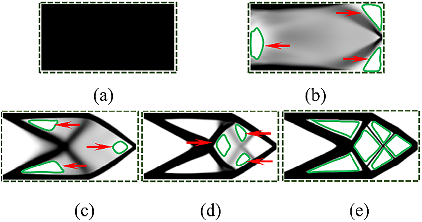
Figure 3: Autonomous pore formation level set method, the process of generating holes in the optimization process: (a) initial structure; (b) preliminary hole structure; (c) hole structure; (d) initial design with holes; (e) clear initial design with holes, and finally clear optimization results are obtained

According to the density-based topology optimization method proposed by Bendsøe et al., the SIMP density function interpolation model is

Ee(xe)=Emin+xep(E0−Emin),xe∈[0,1],(3)

where E0 is the stiffness of the material, Emin is a very small stiffness assigned to hole regions in order to prevent the stiffness matrix from becoming singular, p is a penalization factor, and p is a penalization factor for which a value of 3 is recommended [18], xe is the density of each element e and Ee is the Young’s modulus of each element e.

Using minimum compliance as the objective function, the optimization model is formulated as:

minx:c(x)=UTKU=∑e=1NEe(xe)ueTk0ue,subject to :V(x)−V0≤0,KU=F,0≤x≤1.(4)

In this formulation, c denotes the structural compliance, U and F are the global displacement and external force vectors, respectively; K is the assembled global stiffness matrix, ue is the displacement vector of element, k0 is stiffness matrix for unit Young’s modulus Ee, x is the vector of design variables, N is the total number of finite elements, V(x) and V0 stand for the current material volume and the prescribed volume limit, respectively.

The sensitivities of the objective function c and the material volume V with respect to the element densities xe are provided by:

∂c∂xe=−pxep−1(E0−Emin)ueTk0ue,∂V∂xe=1.(5)

Sensitivity filtering is applied to prevent the occurrence of the checkerboard phenomenon.

∂c^∂xe=∑d=1NH^dxd∂c∂xdxe∑d=1NH^d,(6)

where d denotes the index of neighboring elements located within the filtering radius of element e. The operator H^d represents the spatial weight factor, which is commonly based on the Euclidean distance between element e and element d.

xenew ={max(0,xe−r) if xeBeη≤max(0,xe−r),min(1,xe+r) if xeBeη≥min(1,xe−r),xeBeη otherwise,(7)

where xenew  represents the updated design variable, xe denotes the current design variable, r is the positive move limit, η(=1/2) is the numerical damping coefficient. Based on these definitions, the optimality condition can be formulated as Be [19,20]

Be=−∂c∂xeλ∂V∂xe.(8)

In Eq. (4), λ is the Lagrange multiplier, which is solved by the dichotomy. Through the iterative update of the OC, the material distribution gradually evolves toward an optimal state under the given constraints. Throughout the optimization, the formation of pores naturally results from the material removal strategy embedded in the SIMP-based topology optimization method, as illustrated in Fig. 3.

In this process, elements that are critical to the primary load transfer path are preserved, while those with lower structural significance are progressively removed. As a result, holes form naturally within the design domain without any predefined initialization. The green regions marked by red arrows in Fig. 3a–d indicate the locations of these autonomously generated pores as shown in Fig. 3e.

From Fig. 3d,e, the clearer topological boundaries are obtained by further processing the grayscale SIMP results through a binarization threshold algorithm. This process classifies the global density field into two categories: elements with density values greater than a specified threshold are assigned as solid, while those below are treated as hole. The binarization threshold algorithm is defined as:

B(i,j)={1,ifx(i,j)>κ0,otherwise∀(i,j)∈τ(9)

where τ={(i,j)|0.5≤i≤m−0.5,0.5≤j≤n−0.5} represents the set of all element indices, where m is the number of rows and n is the number of columns in the grid. κ∈(0,1) is the binary threshold, which is determined iteratively using the bisection method to ensure that the binarized structure retains the same material volume as the original density field. The specific process from grayscale to clarity is shown in Fig. 4.

Figure 4: Force transmission path of cantilever beam and binary topology structure

As illustrated in Fig. 4a, a large portion of the initial solution consists of elements with intermediate density values, particularly near structural boundaries, which may hinder subsequent geometric representation and numerical processing. To overcome this limitation, a binary thresholding strategy is applied to eliminate grayscale ambiguity and to generate a distinct solid–hole topology, as illustrated in Fig. 4b [21].

The outcome of this binarization process is a clean and well-defined structural layout, suitable for further geometric treatment. In particular, the resulting binary structure serves as a numerically consistent initial configuration for initializing the subsequent level set function, thereby ensuring topological coherence and continuity across the optimization stages.

To obtain excellent optimization results, it is necessary to obtain a suitable pore structure to ensure the complex topology, Therefore, a judgment threshold is adopted to identify the initial hole configuration [22], as illustrated in Fig. 3d, where the threshold value is calculated following in Eq. (10).

αe=∑k=1Necold,k∑k=1Neck,(10)

where αe is the judgment threshold, cold,k is the objective function before optimization, and ck is the current objective function before optimization. The determination of the judgment threshold will be elaborated in the subsequent section.

2.3 Mapping from Density Field to Level Set Function

To establish a unified geometric representation and enable the mapping from the density field to the level set field, the clearly defined topology obtained through SIMP optimization is first processed to extract its boundary geometry [23], as illustrated in Fig. 5a,b. Based on the identified boundary and surrounding non-boundary regions, a boundary distance model is then constructed, as shown in Fig. 5c. This model provides the foundation for generating the signed distance field, thereby converting the discrete density-based topology into an implicit level set formulation and facilitating seamless transition between the two optimization stages.

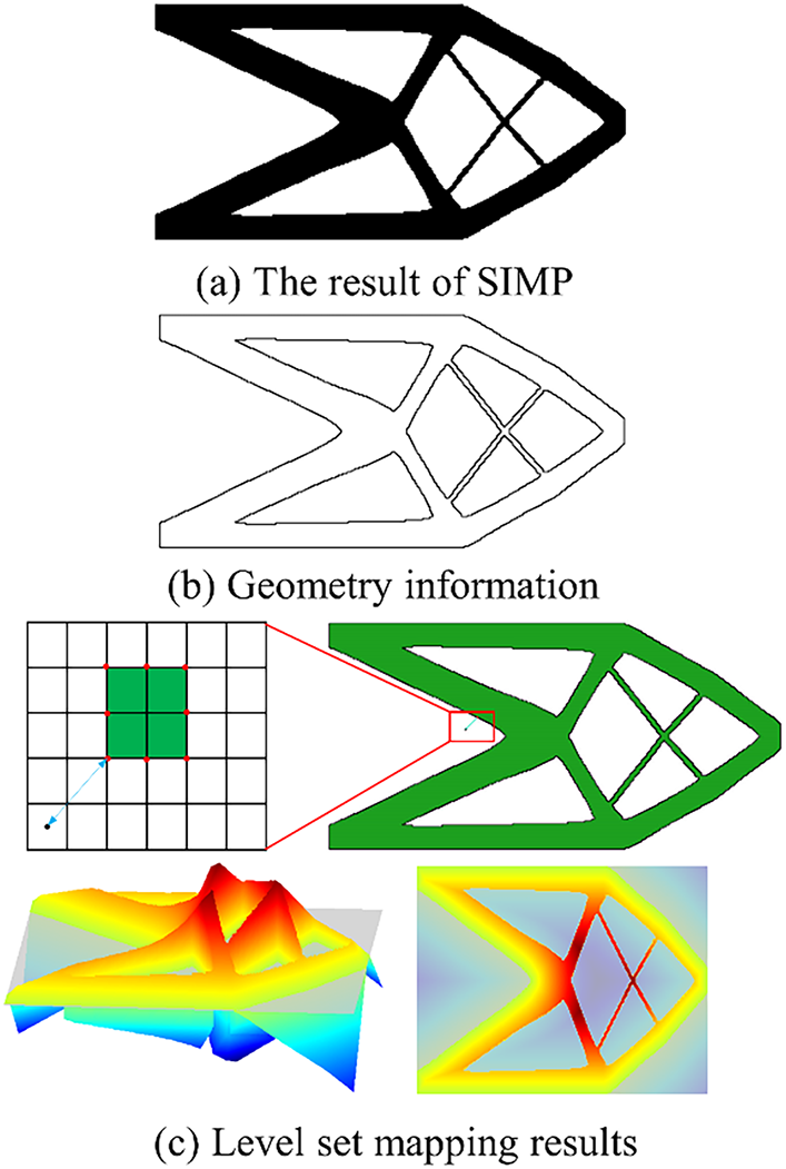
Figure 5: Optimized level set-field mapping process for cantilever beam topology

2.3.1 Extract the Boundary Geometry

To describe the principle of the boundary distance model, the boundary distance is defined as the relationship between the distance from the center point B of the cell to the boundary node A, as shown in Fig. 6.

Figure 6: Schematic diagram of boundary distances

The Fig. 6 represents the boundary distance function, B is the cell coordinate and A is the boundary node coordinate.

To extract the boundary geometry from the binary density distribution, according to Eq. (9), a cell x¯(i,j) is assumed to be a binarized density cell value, and a cell is designated as a boundary cell if at least one of its four neighboring cells has a different state indicating that the cell is in a transition state between solid and hollow. The boundary cell identification function is defined as follows:

C(i,j)={1,∃(p,q)∈N(i,j),B(p,q)≠x¯(i,j),0,otherwise,(11)

where N(i,j)={(i−1,j),(i+1,j),(i,j−1),(i,j+1)} indicates whether the node at C(i,j) is a boundary node (1 for yes and 0 for no). After identifying the set of boundary nodes, the next step is to compute the coordinates of each element center, which are required for the subsequent calculation of boundary distances.

Based on the obtained boundary cells are transformed into boundary nodes defined as:

A={(x,y)|C(i,j)=1},(12)

where (x,y)=(i−0.5,j−0.5) is representing the boundary node coordinates.

2.3.2 Geometry Mapping for Level Set Initialization

Based on the above unit center coordinates and boundary node coordinates, a signed distance function (SDF) is constructed as the initial level set. The boundary distance is defined as the minimum Euclidean distance from the center of the cell to the boundary, as follows:

ϕ(i,j)=sign(B(i,j))⋅min(x,y)∈A(x−i)2+(y−j)2,(13)

here ϕ(i,j) is the boundary distance function, where sign(B(i,j)) determines the point is positive (inside the boundary geometry), negative (outside the boundary geometry) and zero (on the boundary geometry). To ensure consistent geometric sign information, the obtained boundary function is employed to initialize the level set function, as follows:

ϕ(i,j)=Φ(i,j),(14)

where Φ(i,j) is the level set function, which acts as the initial setup for the succeeding topology optimization procedure.

2.3.3 Gaussian Filtering with Level Set Functions

To reduce the effects of protrusions, sharp corners, jagged edges, and numerical oscillations during the transition from the density field to the level set field, Gaussian filtering is introduced to ensure a smooth transition. The Gaussian filtering function is defined as follows:

Φsmooth (i,j)=(G∗Φ)(i,j)=∑g,hG(g,h)Φ(i−g,j−h),(15)

here, Gaussian core is G(i,j)=12πσ2exp⁡(−i2+j22σ2), σ is Gaussian kernel standard deviation; g indicates relative movement in the vertical direction; h indicates relative movement in the horizontal direction.

The level set function in Fig. 7 is Gaussian filtered to achieve a smoothing effect, which effectively reduces the high-frequency noise and details in the image or mesh, and makes the isosurfaces of the level set function more continuous and regular, which is helpful for the subsequent optimization process.

Figure 7: Gaussian filter plot for level set function

The LSM-AHF method achieves a globally reasonable topology distribution while ensuring smooth and manufacturable boundaries.

2.4 Optimization Problem

Building upon the initialized level set function derived above, the topology optimization problem aiming to minimize structural compliance is formulated as follows [24,25]:

min:⁢J=∫Ωεi⁢j⁢(u)⁢Ci⁢j⁢k⁢l⁢εk⁢l⁢(u)⁢dΩ,s.t.:⁢{a⁡(u,v)=l⁡(v),∀v∈Ua⁡dV⁡(Ω)=V∗,(16)

where J is the compliance of the structure, ε is the strain tensor, Cijkl is the fourth-order constitutive tensor, u is the real displacement field, Ω is the area occupied by the linear elastic material, v is the imaginary displacement field, Uad denotes the virtual displacement space, the solid material volume V, and the prescribed target volume V∗. The formulations of the internal and external virtual energies a(u,v) and l(v), respectively, are expressed as follows:

V(Ω)=∫DH(Φ)dΩ,a(u,v)=∫Ωεij(u)Cijklεkl(v)dΩ,l(v)=∫Ωf⋅vdΩ+∫ΓNg⋅vdΓ,(17)

where D is the design domain; H(Φ) is the Heaviside function [26]; Γ=∂Ω for the boundaries of the design domain; a(u,v) is a symmetric bilinear function with respect to the displacement u and the test function v; Under the Neumann boundary condition ΓN, l is a linear function of physical strength f and traction g.

2.5 Sensitivity Analysis

Sensitivity analysis based on shape derivatives was performed under the LSM method optimization framework and the shape sensitivity analysis is derived by adjoint sensitivity analysis in this section. The first step gives the Lagrangian formula for the optimization problem [1,2]:

L(u,v)=J+a(u,v)−l(v)+λ(V(Ω)−V∗),(18)

where λ is the Lagrangian multiplier, which v is the accompanying displacement in the adjoint sensitivity analysis. Eq. (15) can be reformulated as:

L(u,v)=a(u,u)+a(u,v)−l(v)+λ(V(Ω)−V∗).(19)

Eq. (16) is expressed as the material derivative of pseudo-time t as

dL(u,v)dt=∂L(u,v)∂t+∂L(u,v)∂Ω,(20)

where the partial derivative of time gives the so-called adjoint equation:

∂L(u,v)∂t=L′=a′(u,u)+a′(u,v),(21)

and

a′(u,u)=2∫Ωεij(u′)Cijklεkl(u)dΩ,a′(u,v)=∫Ωεij(u′)Cijklεkl(v)dΩ.(22)

The convective component of the material derivative constitutes the shape derivative, which is expressed as:

∂L(u,v)∂Ω=∫Γεij(u)Cijklεkl(u)vnds+∫Γεij(u)Cijklεkl(v)vnds−∫Γf⋅vvnds−∫Γ[∂(g⋅v)∂n+κg⋅v]vnds+λ∫Γvnds.(23)

Solve Eq. (18) to get the adjoining variable v=−2u. Substitute (20) v=−2u, ignore physical strength, and obtain

∂L(u,v)∂Ω=∫Γ[εij(u)Cijklεkl(u)+λ]vnds,(24)

the normal velocity field is formulated based on the steepest descent method as follows.

Vn=−εij(u)Cijklεkl(u)−λ.(25)

Among them, λ for the Lagrangian multiplier that controls the volume constraints, εij(u)Cijklεkl(u) is the strain energy density of the linear elastic structure. Through continuous update speed Vn, the iterative optimization of the structure is realized [17,27].

2.6 Numerical Implementation

This section provides a detailed explanation of the optimization procedure for the LSM-AHF method.

The proposed method (LSM-AHF) uses the SIMP material removal scheme to open holes in the low strain energy region to achieve automatic hole nucleation, eliminating the influence of the initial design on the optimized design, as described in Section 2. The method framework is decomposed into 7 steps, as shown in Algorithm 1.

3  Numerical Examples

3.1 Example of a 2D Optimization Study

To reflect the efficacy and reliability of the LSM-AHF method, verification was conducted using both 2D and 3D examples.

3.1.1 Cantilever Beam

Take a cantilever beam as an example, as shown in Fig. 8. The design domain is discretized into 160 × 80 quadrilateral elements, with the left boundary fixed and a downward force F=1N  applied at the right midpoint. The Young’s modulus of the solid material is assigned as E0=1, while to prevent numerical singularities, the Young’s modulus of the hole material is specified as Emin=10e−9. The Poisson’s ratio is set to u=0.3 and a volume fraction constraint of 0.4 is imposed.

Figure 8: Design domains and boundary conditions for cantilever beam structures

Based on the boundary conditions and load information, the cantilever beam is optimized by the LSM-AHF method and the resulting optimization iteration diagram, shown in Fig. 9.

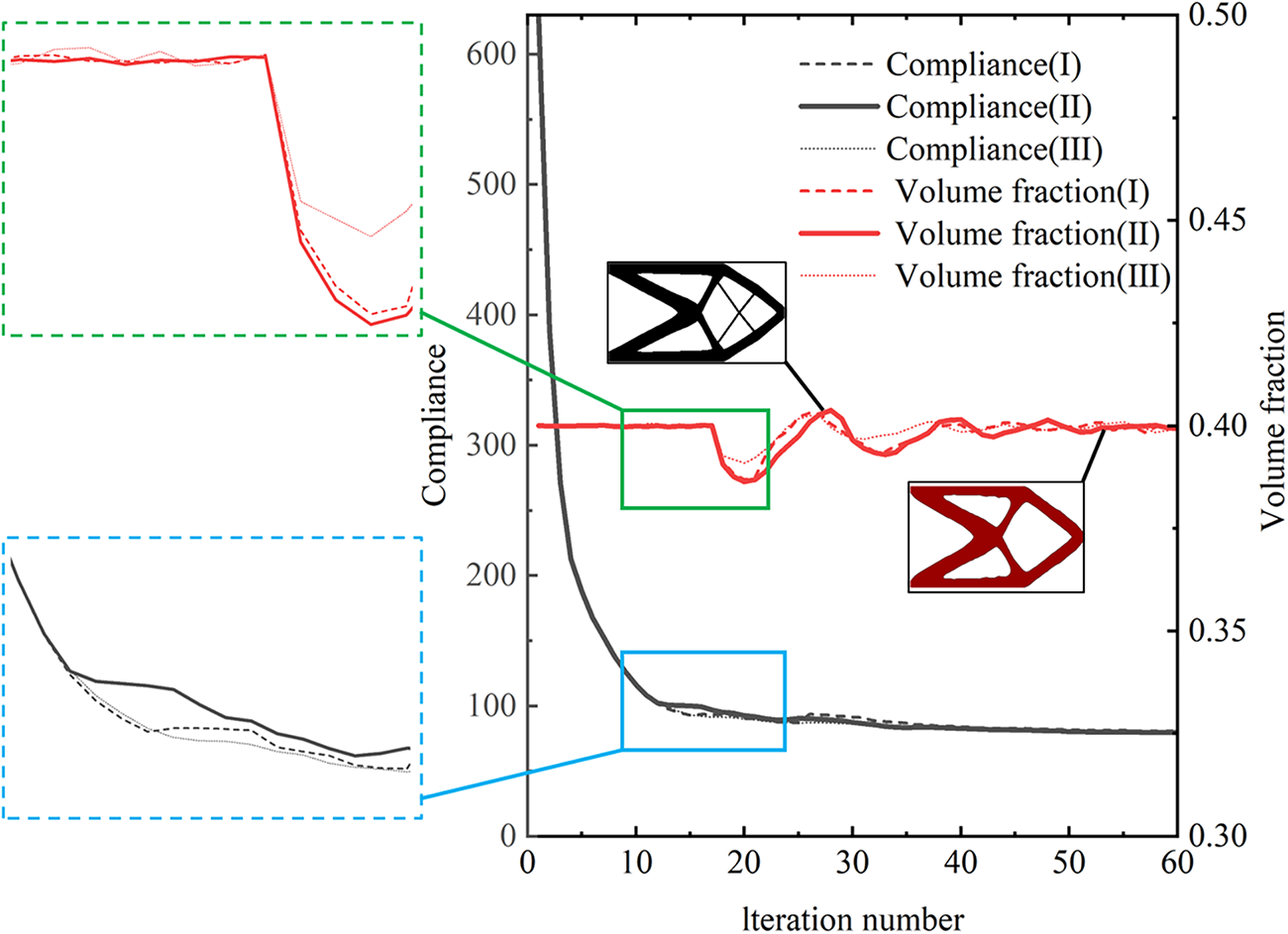
Figure 9: Optimized the historical iteration graph of the cantilever beam topology optimization under different grid resolutions: Grid I (120 × 60), Grid II (160 × 80), and Grid III (200 × 100)

As can be seen from Fig. 9, when the threshold is 0.05, the value of the objective function remains stable after only 28 iterations, indicating that the convergence condition is reached relatively quickly in this case. Moreover, consistent convergence behavior across different grid resolutions further demonstrates the robustness and reliability of the LSM-AHF method.

Taking the cantilever beam structure as an example, the effect of different judgment thresholds on the optimization results is investigated by the LSM-AHF topology optimization method proposed in this paper as shown in Table 1.

The optimization process of the cantilever beam topology under different judgment thresholds is analyzed based on Table 1. As the judgment threshold increases, the number of iterations decreases while the final compliance increases, indicating a trade-off between computational efficiency and solution quality. Specifically, when αe=0.05, both the objective function value (compliance) and the volume fraction stabilize after approximately 83 iterations. Although this setting requires a longer convergence time, it yields a relatively low compliance value, suggesting that an optimal structural topology is achieved. This suggests that lower thresholds (αe≤0.1) are more suitable for accuracy-demanding scenarios.

To verify the performance of the proposed LSM-AHF method, the VFLS (Velocity field level-set) method with different initial designs is comparatively analyzed as shown in Table 2.

Using the VFLS method to compare the initial design 1 and initial design 2 forms uniformly in the design domain, the optimization results are shown in Table 2, it is evident that the topology obtained from initial design 1 is suboptimal, as indicated by a relatively high structural compliance of 73.991, while the topology results obtained from Initial Design 2 yield a compliance value of 72.988, the compliance values produced by the LSM-AHF method are closely aligned with those of the VFLS method, with a difference of less than 6.5%. This consistency verifies the robustness of the proposed method.

3.1.2 Messerschmitt-Bolkow-Blohm (MBB) Beam

The optimal design problem for the MBB beam is illustrated in Fig. 10. The beam is subjected to a vertical force applied at the midpoint of its upper edge. The reference domain for this problem is a rectangular area measuring 2 × 1 units. The upper limit for the volume fraction in this design is set at 0.4 [28].

Figure 10: Design domain and boundary conditions of the MBB beam structure

The optimization iteration process of the MBB beam is carried out using the LSM-AHF method, and the corresponding iteration results are shown in Fig. 11.

Figure 11: Optimized the historical iteration graph of the MBB beam under different grid resolutions: Grid I (120 × 60), Grid II (160 × 80), and Grid III (200 × 100)

The iterative trends of the objective function and volume fraction are illustrated in Fig. 11. After the initial 15th iterations, the objective function gradually stabilizes. This stabilization can be attributed to the initial design’s ability to automatically generate holes and evolve into a more complex topological configuration, which is effectively captured by the LSM-AHF framework, thereby enhancing the convergence and optimization performance. A numerical oscillation is observed around the 20th iteration, which is caused by the transition from the density field to the level set field. Moreover, the convergence behavior is observed to be consistent across different grid resolutions, indicating the reliability of the LSM-AHF method in capturing the optimization trends.

The optimization process of the cantilever beam topology under different judgment thresholds is analyzed based on Table 3. As the judgment threshold increases, the number of iterations decreases while the final compliance increases. Specifically, when αe=0.05, both the objective function value (compliance) and the volume fraction stabilize after approximately 38 iterations. Although this setting requires a longer convergence time, it yields a relatively low compliance value, suggesting that an optimal structural topology is achieved.

To evaluate the performance of the proposed LSM-AHF method, a comparative analysis was conducted using the VFLS method applied to MBB beams with different initial designs, as summarized in Table 4.

Using the VFLS method to compare the initial design 1 and initial design 2 forms uniformly in the design domain, the optimization results are shown in Table 4, it is obvious that the topology results obtained by the initial design 1 are not very ideal, with a structural compliance of 15.887; while the topology results obtained by the initial design 2 have a compliance value of 15.843, and the structural compliance values obtained by the LSM-AHF method are close to those obtained by the VFLS method, which verifies the compliance of the method.

3.1.3 Cantilever Beam with Fixing Holes

A cantilever beam featuring fixing holes, subjected to a vertical load F=1N  applied to its lower right section. The reference domain is a rectangle measuring 2 × 1 units, with a volume fraction upper limit of 0.4, as shown in Fig. 12.

Figure 12: Design domains and boundary conditions for cantilever structures with fixing holes

The optimization iteration process of the cantilever beam with fixing holes is carried out using the LSM-AHF method, and the corresponding iteration results are shown in Fig. 13.

Figure 13: Optimized historical iteration graphs for cantilever structures with fixing holes under different grid resolutions: Grid I (120 × 60), Grid II (160 × 80), and Grid III (200 × 100)

The cantilever beam with fixing holes is optimized using the LSM-AHF method. As shown in Fig. 13, a noticeable numerical oscillation in the volume fraction occurs around the 13th iteration, which is attributed to the mapping process from the density field to the level set field. The solution quickly stabilizes in the subsequent iterations, demonstrating the fast convergence capability of the proposed method. Moreover, the results are consistent across different grid resolutions, confirming the robustness of the observed convergence behavior.

To evaluate the performance of the proposed LSM-AHF method, a comparative analysis was conducted using the VFLS method applied to cantilever beam with fixing holes with different initial designs, as summarized in Table 5.

The optimization process of the cantilever beam topology under different judgment thresholds is analyzed based on Table 5. As the judgment threshold increases, the number of iterations decreases while the final compliance increases. Specifically, when αe=0.05, both the objective function value (compliance) and the volume fraction stabilize after approximately 60 iterations. Although this setting requires a longer convergence time, it yields a relatively low compliance value, suggesting that an optimal structural topology is achieved.

To evaluate the performance of the proposed LSM-AHF method, a comparative analysis was conducted using the VFLS method applied to MBB beams with different initial designs, as summarized in Table 6.

Using the VFLS method to compare the initial design 1 and initial design 2 forms uniformly in the design domain, the optimization results are shown in Table 6, it is obvious that the topology results obtained by the initial design 1 are not very ideal, with a structural compliance of 88.053; while the topology results obtained by the initial design 2 have a compliance value of 89.053, and the structural compliance values obtained by the LSM-AHF method are close to those obtained by the VFLS method, which verifies the compliance of the method.

The initial SIMP stage rapidly identifies the main load-carrying paths, providing a good starting point. The subsequent LSM stage only needs to refine boundaries and optimize topology locally, which is not significantly increase computational time.

3.2 3D Optimization Study

3.2.1 Cantilever Beam Structure

As shown in Fig. 14, a three-dimensional cantilever beam with a reference size of 4 × 4 × 2 is analyzed. A vertical load F=1N  is imposed at the midpoint of its right end, and the structure must satisfy a volume constraint of 0.4 [29,30].

Figure 14: Design domains and boundary conditions for the 3D cantilever structures

The iterative journey of the objective function is shown in Fig. 15. In the first 12 to 45 iterations, the value of the objective function oscillates, mainly due to the vigorous motion during the hole fusion process, evolving a complex topology from a basic topology.

Figure 15: Optimized historical iteration graphs of the 3D cantilever structures

3.2.2 Three-Dimensional Simply Supported Structure

As shown in Fig. 16, the case study considers a simply supported 3D structure with dimensions of 4 × 4 × 4, subjected to a vertical load F=1N  at the midpoint of the top face, with a volume constraint set at 0.4.

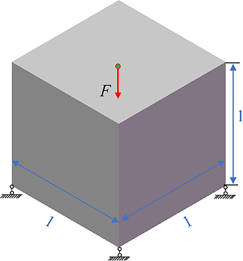
Figure 16: Design domains and boundary conditions for the 3D supported structure

The iterative journey of the objective function is shown in Fig. 17. in the first 25 to 35 iterations, the value of the objective function oscillates, mainly due to the vigorous motion during the hole fusion process, generating a complex topology from a trivial topology. Moreover, the LSM-AHF method can be readily extended to the design of composite and graded material structures [31,32]. With more flexible encoding strategies, it can also be applied to the optimization of GPL (Graphene Platelet) distributions and different foundation types, thereby broadening its applicability.

Figure 17: Optimized historical iteration graphs of the 3D supported structure

4  Conclusion

To address the limitation of the level set method (LSM) in autonomously generating new holes during topological evolution, a novel level set-based topology optimization method with autonomous hole formation capability (LSM-AHF) is introduced in this research The approach first applies a judgment threshold to the SIMP density field to obtain a clearly defined porous initial design. Then, the boundary of this porous initial design is extracted and used to construct a signed distance model, enabling a consistent and accurate mapping from the density field to the level set field. This mapping allows the design to smoothly transition into the LSM framework for further structural optimization. Numerical examples demonstrate that the proposed LSM-AHF significantly improves topological adaptability and optimization effectiveness. By addressing the hole-nucleation limitation of traditional LSM and resolving the boundary irregularity of SIMP-based designs, the method offers a robust and unified solution for topology optimization with enhanced geometric and structural performance. Future work will focus on incorporating experimental validation to calibrate material parameters and verify optimized designs, thereby enhancing the reliability and applicability of the proposed framework. Moreover, the proposed method is general and can be extended to other types of composite structures, different geometries, and diverse loading scenarios.

Acknowledgement: None.

Funding Statement: This work was supported by the National Natural Science Foundation of China [52475096]; Guangxi Natural Science Fund for Distinguished Young Scholars [2025GXNSFFA069009]; Bagui Outstanding Youth Program of Guangxi, China; Natural Science and Technology Innovation Development Doubling Plan Project of Guangxi University, China [2024BZRC010]; Innovation Project of Guangxi Graduate Education, China [YCBZ2025014].

Author Contributions: Fei Wu developed the research framework, performed theoretical derivations, and drafted the manuscript. Ziyang Zeng conducted result interpretation and revised the manuscript accordingly. Kunliang Xie prepared the figures and conducted data analysis. Yuqiang Liu contributed to the development of the research manuscript revisions. Jiang Ding contributed to the research framework and manuscript preparation. All authors reviewed the results and approved the final version of the manuscript.

Availability of Data and Materials: The data that support the findings of this study are available from the corresponding author upon reasonable request.

Ethics Approval: Not applicable.

Conflicts of Interest: The authors declare no conflicts of interest to report regarding the present study.

References

1. Allaire G, Jouve F, Toader AM. Structural optimization using sensitivity analysis and a level-set method. J Comput Phys. 2004;194:363–93. doi:10.1016/j.jcp.2003.09.032. [Google Scholar] [CrossRef]

2. Mei Y, Wang X. A level set method for structural topology optimization and its applications. Adv Eng Softw. 2004;35:415–41. doi:10.1016/j.advengsoft.2004.06.004. [Google Scholar] [CrossRef]

3. Van Dijk NP, Maute K, Langelaar M, Van Keulen F. Level-set methods for structural topology optimization: a review. Struct Multidisc Optim. 2013;48:437–72. doi:10.1007/s00158-013-0912-y. [Google Scholar] [CrossRef]

4. Wang MY, Wang X, Guo D. A level set method for structural topology optimization. Comput Methods Appl Mech Eng. 2003;192:227–46. doi:10.1016/S0045-7825(02)00559-5. [Google Scholar] [CrossRef]

5. Eschenauer HA, Kobelev VV, Schumacher A. Bubble method for topology and shape optimization of structures. Struct Optim. 1994;8:42–51. doi:10.1007/BF01742933. [Google Scholar] [CrossRef]

6. Burger M, Hackl B, Ring W. Incorporating topological derivatives into level set methods. J Comput Phys. 2004;194:344–62. doi:10.1016/j.jcp.2003.09.033. [Google Scholar] [CrossRef]

7. Cai S, Zhang W. An adaptive bubble method for structural shape and topology optimization. Comput Methods Appl Mech Eng. 2020;360:112778. doi:10.1016/j.cma.2019.112778. [Google Scholar] [CrossRef]

8. Challis VJ. A discrete level-set topology optimization code written in Matlab. Struct Multidisc Optim. 2010;41:453–64. doi:10.1007/s00158-009-0430-0. [Google Scholar] [CrossRef]

9. Wei P, Li Z, Li X, Wang MY. An 88-line MATLAB code for the parameterized level set method based topology optimization using radial basis functions. Struct Multidisc Optim. 2018;58:831–49. doi:10.1007/s00158-018-1904-8. [Google Scholar] [CrossRef]

10. Luo J, Luo Z, Chen L, Tong L, Wang MY. A semi-implicit level set method for structural shape and topology optimization. J Comput Phys. 2008;227:5561–81. doi:10.1016/j.jcp.2008.02.003. [Google Scholar] [CrossRef]

11. Ullah B. A coupled meshless element-free galerkin and radial basis functions method for level set-based topology optimization. J Braz Soc Mech Sci Eng. 2022;44(3):89. doi:10.1007/s40430-022-03382-5. [Google Scholar] [CrossRef]

12. Ullah B, Ullah Z, Khan W. A parametrized level set based topology optimization method for analysing thermal problems. Comput Math Appl. 2021;99:99–112. doi:10.1016/j.camwa.2021.07.018. [Google Scholar] [CrossRef]

13. Oellerich J, Yamada T. A level set topology optimization theory based on Hamilton’s principle. Int J Numer Methods Eng. 2025;126(17):e70120. [Google Scholar]

14. Xia Q, Shi T, Xia L. Stable hole nucleation in level set based topology optimization by using the material removal scheme of BESO. Comput Methods Appl Mech Eng. 2019;343:438–52. doi:10.1016/j.cma.2018.09.002. [Google Scholar] [CrossRef]

15. Zong Z, Shi T, Xia Q. A parameter-free approach to determine the lagrange multiplier in the level set method by using the BESO. Comput Model Eng Sci. 2021;128:283–95. doi:10.32604/cmes.2021.015975. [Google Scholar] [CrossRef]

16. Park KS, Youn SK. Topology optimization of shell structures using adaptive inner-front (AIF) level set method. Struct Multidisc Optim. 2008;36:43–58. doi:10.1007/s00158-007-0169-4. [Google Scholar] [CrossRef]

17. Ding J, Zeng Z, Xing Z, Nong W, Wu F. Discrete level set method enhanced by conformal mapping: an efficient approach for topology optimization of piezoelectric energy harvesters. Struct Multidisc Optim. 2024;67:173. doi:10.1007/s00158-024-03893-w. [Google Scholar] [CrossRef]

18. Rozvany GIN, Zhou M. The COC algorithm, part I: cross-section optimization or sizing. Comput Methods Appl Mech Eng. 1991;89:281–308. doi:10.1016/0045-7825(91)90045-8. [Google Scholar] [CrossRef]

19. Andreassen E, Clausen A, Schevenels M, Lazarov BS, Sigmund O. Efficient topology optimization in MATLAB using 88 lines of code. Struct Multidisc Optim. 2011;43:1–16. doi:10.1007/s00158-010-0594-7. [Google Scholar] [CrossRef]

20. Ming Zhou, Sigmund O. Complementary lecture notes for teaching the 99/88-line topology optimization codes. Struct Multidiscip Optim. 2021;64(5):3227–31. doi:10.1007/s00158-021-03004-z. [Google Scholar] [CrossRef]

21. Zhang J, Liu E, Liao J. An explicit and implicit hybrid method for structural topology optimization. J Phys. 2021;1820:012183. doi:10.1088/1742-6596/1820/1/012183. [Google Scholar] [CrossRef]

22. Huang X, Xie YM. Evolutionary topology optimization of continuum structures: methods and applications. 1st ed. Hoboken, NJ, USA: John Wiley & Sons, Inc.; 2010. doi:10.1002/9780470689486. [Google Scholar] [CrossRef]

23. Garrido-Jurado S, Muñoz-Salinas R, Madrid-Cuevas FJ, Marín-Jiménez MJ. Automatic generation and detection of highly reliable fiducial markers under occlusion. Pattern Recognit. 2014;47:2280–92. doi:10.1016/j.patcog.2014.01.005. [Google Scholar] [CrossRef]

24. Wang Y, Kang Z, Liu P. Velocity field level-set method for topological shape optimization using freely distributed design variables. Int J Numer Methods Eng. 2019;120:1411–27. doi:10.1002/nme.6185. [Google Scholar] [CrossRef]

25. Cui M, Luo C, Li G, Pan M. The parameterized level set method for structural topology optimization with shape sensitivity constraint factor. Eng Comput. 2021;37:855–72. doi:10.1007/s00366-019-00860-8. [Google Scholar] [CrossRef]

26. Osher S, Sethian JA. Fronts propagating with curvature-dependent speed: algorithms based on Hamilton-Jacobi formulations. J Comput Phys. 1988;79:12–49. doi:10.1016/0021-9991(88)90002-2. [Google Scholar] [CrossRef]

27. Ding J, Xing Z, Zeng Z, Nong W, Wu F. Level set function based on conformal geometry theory: an efficient approach for optimization of shell structure with arbitrary gaussian curvature. Structures. 2023;56:104995. doi:10.1016/j.istruc.2023.104995. [Google Scholar] [CrossRef]

28. Luo Z, Tong L, Kang Z. A level set method for structural shape and topology optimization using radial basis functions. Comput Struct. 2009;87:425–34. doi:10.1016/j.compstruc.2009.01.008. [Google Scholar] [CrossRef]

29. Deng H, Vulimiri PS, To AC. An efficient 146-line 3D sensitivity analysis code of stress-based topology optimization written in MATLAB. Optim Eng. 2022;23:1733–57. doi:10.1007/s11081-021-09675-3. [Google Scholar] [CrossRef]

30. Gao J, Yang Z, Zhang Y, Liu S. An improved partial differential equation filter scheme for topology optimization of additively manufactured coated structure. Comput Struct. 2023;288:107147. doi:10.1016/j.compstruc.2023.107147. [Google Scholar] [CrossRef]

31. Banh TT, Lee D. Multi-material topology optimization design for continuum structures with crack patterns. Compos Struct. 2018;186:193–209. doi:10.1016/j.compstruct.2017.12.004. [Google Scholar] [CrossRef]

32. Banh TT, Lieu QX, Lee J, Kang J, Lee D. A robust dynamic unified multi-material topology optimization method for functionally graded structures. Struct Multidiscip Optim. 2023;66(4):75. doi:10.1007/s00158-023-03410-3. [Google Scholar] [CrossRef]