Spectrotemporal Deep Learning for Heart Sound Classification under Clinical Noise Conditions

1  Introduction

Cardiovascular diseases (CVDs) refer to a wide variety of conditions that impact the cardiovascular system, which comprises the vascular system that supplies the brain and other critical organs. Such diseases are the primary cause of mortality and morbidity globally [1], a fact that highlights the dire need for accurate and early diagnostic tools. For the effective treatment and management of cardiovascular diseases (CVDs), the early diagnosis of cardiac pathologies and their detection utilizing accurate phenotypes is of paramount importance [2]. Standard diagnostic methods depend on clinicians’ manual interpretation, which is often subjective and susceptible to inter-observer variability [3]. On the other hand, artificial intelligence (AI)-based frameworks, particularly those utilizing machine and deep learning algorithms, offer a promising alternative for consistent and objective CVD analysis and management [4,5]. Phonocardiography (PCG) and electrocardiography (ECG) are two of the most common non-invasive methods that are used to monitor the activity of the heart [6]. While the ECG captures the bioelectrical conduction through the heart muscle tissue, the PCG records the sounds that are produced by the movement of the heart valves and the heart muscle [7]. In low-resource or rural settings, PCG holds particular clinical utility over ECG primarily due to its simpler and low-cost hardware requirements compared to ECG [8]. It also enables non-invasive and rapid cardiac screening without the need for electrode placement or complex calibration [9].

In recent years, advancements in deep learning, particularly with Convolutional Neural Networks (CNNs), have significantly advanced fields such as biomedical signal processing [10,11]. CNNs excel at identifying complex patterns and features within data making them particularly well-suited for tasks like PCG signal classification [12,13]. However, the effectiveness of CNNs is heavily dependent on the quality of feature extraction from raw signals. Mel Spectrograms, a technique originally developed for audio processing [14], provide a time-frequency representation that captures both the temporal dynamics and spectral characteristics of an acoustic signal [15]. Applying Mel Spectrograms to PCG data transforms the raw acoustic signals into an image-like representation that enhances the discriminative capabilities of CNNs [16]. In addition, the combination of ECG and PCG data has the potential to vastly enhance diagnostic precision by offering further insights into the electrical and mechanical processes of the heart [17], however, it necessitates that both tools must be available, which is typically not the case at consumer settings or low-resource environments.

In real-world clinical environments, PCG recordings are often polluted by a variety of noises, including ambient conversations, sounds from hospital equipment, and motion artifacts [18]. This noise has the potential to drastically reduce the quality of PCG signals, thereby diminishing the efficiency of automated classification technologies [19]. To address this challenge, this work simulates realistic clinical settings and analyzes the robustness of the model by integrating a variety of noise types at varying Signal-to-Noise Ratio (SNR) levels.

This study extends prior works by performing a rigorous external validation on a new dataset and investigating critical questions regarding model adaptation and robustness under mixed heart and lung sounds. Our research objectives are to: 1) Evaluate the generalizability of a model trained on the PhysioNet dataset by fine-tuning it on the HLS-CMDS dataset for both binary and multi-class tasks; 2) Compare the efficacy of fine-tuning a domain-specific model vs. retraining a general-purpose (ImageNet) model on the new dataset; and 3) Introduce a novel robustness test to assess the model’s performance on heart sounds computationally separated from mixed recordings, simulating a challenging real-world signal processing scenario. By addressing these objectives, we aim to provide deeper insights into the practical challenges of deploying PCG classification models in clinical environments.

2  Related Works

Unlike Electrocardiogram (ECG) or Photoplethysmogram (PPG) signals, which capture cardiac electrophysiological and volumetric dynamics, respectively, the Phonocardiogram (PCG) can reveal irregularities linked to specific valvular dysfunctions, such as mitral regurgitation (MR), mitral stenosis (MS), and aortic stenosis (AS). However, the clinical utility of PCG is often challenged by its high susceptibility to noise, low signal-to-noise ratio (SNR), and inherent cyclostationary properties, which introduce significant hurdles for automated analysis and classification [18].

A primary challenge in PCG analysis is the reliable extraction of meaningful features in the presence of environmental noise and interference from other physiological signals. Early methods relied heavily on signal filtering and segmentation, but more sophisticated approaches have emerged to address the non-stationary nature of heart sounds. For instance, Ghosh et al. [20] utilized the Chirplet Transform to capture chirp-like features that are symptomatic of various heart valve diseases. They were able to achieve classification accuracies that were greater than 96%, however, the computational complexity of such methods remains a concern. A number of other preprocessing and feature extraction procedures, including multi-resolution wavelet decomposition, mel-frequency cepstral coefficients (MFCCs), and energy-based analysis, have also been investigated in order to identify the most important properties of PCG signals [21].

To improve classification performance, several researchers have investigated the possibility of features fusion from multiple domains. For instance, Li et al. [22] combined time, frequency, energy, and entropy features to create a robust set of descriptors that can be utilized for classification under a wide range of circumstances. Similarly, Tang et al. [23] showed that combining temporal intervals, frequency spectra, and statistical features can greatly increase classification accuracy for normal and abnormal heart sounds, attaining results that are close to 88%. These multi-domain techniques, on the other hand, frequently result in the creation of high-dimensional feature spaces, which creates a greater computational burden and raise the possibility of overfitting, particularly when dealing with limited datasets.

Deep learning has resulted in significant advancements, including architectures capable of learning abstract representations directly from raw or processed PCG signals. For example, Dominguez-Morales et al. [24] developed a system integrating neuromorphic auditory sensors with deep neural networks that exhibited stable performance even in environments with significant background noise. Sotaquira et al. [25] introduced a weighted probability comparison technique within a deep neural network to address the class imbalance issues that are typically encountered in PCG datasets. Convolutional Neural Networks (CNNs), particularly when applied to 2D spectrogram representations of PCG signals, have become a foundation of modern techniques due to their ability to capture local patterns. Studies by Khan et al. [26] and Krishnan and Balasubramanian [27] have shown that CNNs when combined with transfer learning can classify unsegmented PCG spectrograms with high accuracy, provided that preprocessing and segmentation for training are handled carefully.

Additionally, a growing area of interest that focuses on the noise resilience and adaptability of machine learning models in real-world environments is gaining momentum. Chen et al. [28] explored the impact of various Signal-to-Noise Ratio (SNR) levels on classification performance, thus suggesting the need for algorithms that are capable of maintaining accuracy in noisy settings. Similarly, multimodal approaches that combine PCG with other physiological signals, such as ECG, have also shown promise. Milani et al. [29] demonstrated that integration of data from multiple modalities can enhance overall accuracy of the model. To address the limited availability of data, researchers have also explored data augmentation and transfer learning methods in order to enhance the model generalization [30].

In summary, significant efforts in PCG signal classification reflect a multidisciplinary fusion of advanced signal processing, machine learning, and hardware optimization. While time-frequency methods like the Chirplet Transform have proven effective for non-stationary signals [20], and multi-domain feature extraction has been shown to bolster accuracy [22,23], deep learning techniques have achieved state-of-the-art results [24,25]. Despite this progress, challenges related to noise robustness, real-time analysis, model complexity, and generalizability across diverse patient populations persist [28,30].

Despite these advancements, many existing models require large, labeled datasets for training, which are often scarce in the medical domain. Furthermore, models trained on specific datasets may lack generalizability across different populations and recording conditions, limiting their practical applicability. The current state-of-the-art is characterized by deep learning models that leverage spectrogram-based feature extraction. Techniques such as Mel Spectrograms have become standard for transforming audio signals into an image-like format suitable for CNNs, as these representations capture essential time-frequency characteristics. However, several research gaps need to be addressed:

•   Most deep learning models are computationally intensive, posing challenges for real-time diagnostic applications on resource-constrained devices.

•   While multimodal approaches show promise, effectively fusing diverse data types to leverage the strengths of each modality remains a challenge.

•   Limited studies have systematically evaluated the robustness of classification models under the varying noise conditions and SNR levels encountered in real-world clinical environments.

To address these gaps, this study aims to:

1.    Implement robust data preprocessing techniques, including normalization and precise, event-based segmentation.

2.    Introduce various noise types at different SNR levels to simulate realistic clinical recording conditions and assess the impact on model performance.

3.    Utilize Mel Spectrograms to capture complex time-frequency patterns for effective feature learning.

4.    Develop and evaluate a CNN architecture using the PyTorch/PyTorch Lightning framework for multi-class PCG classification under diverse noise conditions.

5.    Conduct hyperparameter tuning and incorporate regularization techniques to optimize model accuracy and prevent overfitting.

6.    Perform a comprehensive SNR-based classification analysis to evaluate model robustness.

7.    Conduct external validation on a separate dataset (HLS-CMDS) to assess model generalizability and compare domain adaptation strategies.

8.    Evaluate model performance on computationally separated heart sounds to test robustness against signal processing artifacts.

By pursuing these objectives, this study seeks to advance the field of automated cardiovascular diagnostics by providing reliable and efficient tools for early disease detection and management. A summary of the key literature is presented in Table 1.

3  Methodology

The end-to-end architecture of the proposed PCG classification framework is illustrated in Fig. 1. Each block is elaborated in the subsequent subsections.

Figure 1: PCG classification system architecture. The end-to-end pipeline processes raw phonocardiogram recordings (n = 2435) through signal preprocessing, Mel spectrogram feature extraction, and ResNet-18 deep learning classification. The system achieves 94.1% validation accuracy and demonstrates robust performance across clinical noise conditions. Mathematical formulations and comprehensive performance metrics are integrated for scientific rigor

3.1 Data Acquisition

The primary dataset utilized for training the model and performing initial validation was the PhysioNet Challenge 2016 dataset [31]. This public repository includes 2435 phonocardiogram (PCG) recordings from a wide range of patient demographics and comprise a comprehensive range of heart diseases. The recordings are categorized into five classes: Aortic Disease (AD), Miscellaneous Pathological Conditions (MPC), Mitral Valve Prolapse (MVP), Benign, and Normal. Each recording is provided as a .wav file, with corresponding annotations stored in .mat files that detail the timing of relevant physiological states. These annotations provide information about the timing of the physiological states that are relevant to the recording.

A second, independent dataset is incorporated into this study for external validation of the proposed methodology. This dataset is known as the Heart and Lung Sounds Dataset Recorded from a Clinical Manikin using a Digital Stethoscope (HLS-CMDS) [32]. This dataset includes 535 recordings that were taken from a high-fidelity clinical manikin that was designed to simulate a wide variety of normal and pathological conditions. To simulate a realistic diagnostic examination, the recordings contain a variety of PCG types, such as Normal Heart, various murmurs, Atrial Fibrillation, and different lung sounds. These recordings were captured from multiple anatomical locations. The use of a manikin provides an acoustic environment that is highly controlled and repeatable. This ensures that the signals are standardized and free from the confounding variables that are frequently present in human recordings (for example, patient movement or inconsistent stethoscope placement). Its inclusion is therefore critical for assessing our model’s generalizability and its ability to classify specific pathologies when presented with data from a different source and modality—a key step toward establishing clinical viability.

3.2 Data Preprocessing and Signal Analysis

Initially, each PCG recording is normalized by scaling its amplitude to a range of [−1, 1] using the following equation:

xnormalized[n]=x[n]max(|x|),(1)

where x[n] is the n-th sample of the original signal and max(|x|) is the maximum absolute amplitude of the entire recording. Following this step of normalization, a segmentation algorithm is applied, which identifies and isolates the first (S1) and second (S2) heart sounds based on the event timings that are provided in the annotations of the dataset.

3.2.1 Signal Segmentation

To extract clinically relevant information, each PCG signal was segmented using event timings obtained from concurrent ECG recordings. The dataset includes annotation files in.mat format that contain discrete timestamps (ti) and corresponding labels (li) for key cardiac events such as the first heart sound (S1), the second heart sound (S2), and diastole, as illustrated in Fig. 2. Our annotation processing pipeline starts with extracting these timestamps and labels. Synchronizing the annotation timestamps with the PCG audio signal’s sample indices is a critical step. This temporal alignment is accomplished through the following relation:

taligned=ti⋅fsfa,(2)

where taligned is the resulting sample index, fs is the sampling frequency of the PCG signal, and fa is the annotation frequency.

Figure 2: PCG signal segmentation and cardiac cycle analysis. Visualization showing phonocardiogram waveform with precise S1/S2 heart sound identification, cardiac phase segmentation (systole/diastole), temporal measurements, and clinical parameters for automated feature extraction

Using these aligned timestamps, the normalized PCG signal is segmented into intervals corresponding to specific cardiac events, as illustrated in Fig. 3. For instance, the systolic phase of the cardiac cycle is isolated by extracting the segment between S1 and S2:

s=x[tS1:tS2],(3)

where x represents the normalized PCG signal, and tS1 and tS2 are the aligned timestamps for the start of the first and second heart sounds, respectively. By restricting the analysis window to these annotated cardiac events, the pipeline ensures that each segment contains physiologically relevant information. This precise segmentation is essential for reducing the influence of noise and improving the accuracy of subsequent feature extraction and classification tasks. The decision to segment the PCG signal to the systolic interval (from S1 to S2) is a deliberate methodological choice. This approach is standard in several PCG analysis studies as it focuses the model’s attention on the window where the majority of diagnostically significant murmurs, such as those caused by mitral regurgitation and aortic stenosis, occur [33,34]. Furthermore, this strategy creates shorter, more uniform data segments, which can reduce computational complexity and minimize the influence of noise that may be present during the longer and more variable diastolic phase [23,35]. While this simplification is effective for detecting systolic pathologies, it intentionally excludes diastolic events, a trade-off that is explicitly evaluated in our external validation experiments.

Figure 3: This figure shows the process of segmentation of PCG signals based on ECG annotations

3.2.2 Simulation of Clinical Noise Conditions

To evaluate the robustness of our model under realistic clinical scenarios, we systematically introduced noise to the clean, segmented PCG signals. We simulated a range of acoustic environments by incorporating three distinct noise types: white Gaussian noise, pink noise, and authentic ambient recordings from a hospital setting.

Each noise type was added to the signals at four different Signal-to-Noise Ratio (SNR) levels: 0, 10, 20, and 30 dB. This process generated a comprehensive set of noisy datasets, enabling a rigorous assessment of the CNN model’s classification performance as a function of both noise intensity and type.

3.3 External Validation on HLS-CMDS Dataset

A distinct preprocessing pipeline was developed for the external validation on the HLS-CMDS dataset to address its unique characteristics: the presence of mixed heart and lung sounds and the absence of concurrent ECG signals for event-based segmentation.

First, to isolate the cardiac component from the mixed recordings, we applied a Butterworth band-pass filter. Based on our exploratory analysis, a pass-band of 25–400 Hz was established to preserve the primary frequency content of heart sounds while attenuating the majority of lung sound energy. We acknowledge that this filtering method is an approximation, as a partial spectral overlap exists between heart and lung sounds, and it may not achieve perfect separation. The outcome of this separation process is illustrated in Figs. 4–6, which display the waveform, Mel spectrogram, and Power Spectral Density (PSD) for the original mixed signal and the separated components.

Figure 4: Analysis of mixed heart and lung sounds. From top to bottom: waveform, Mel spectrogram, and power spectral density (PSD) of the original mixed signal from the HLS-CMDS dataset

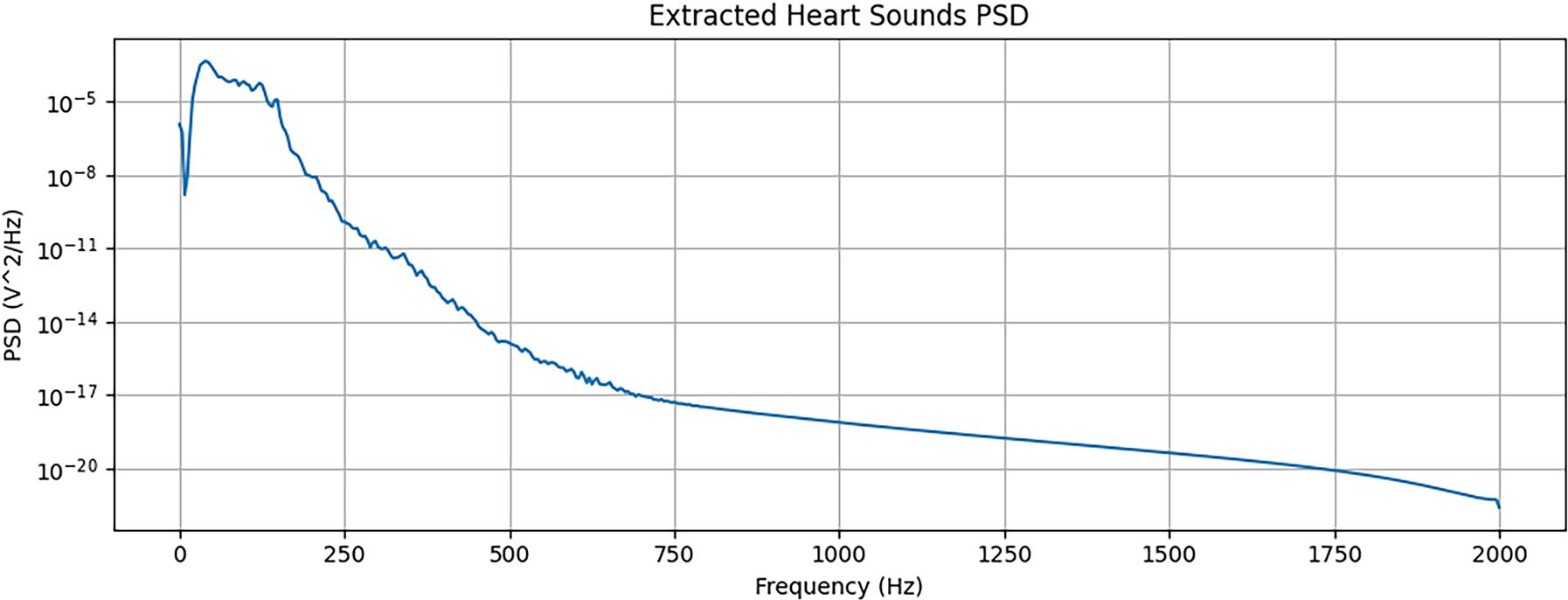
Figure 5: Analysis of extracted heart sounds. From top to bottom: waveform, Mel spectrogram, and PSD of the heart sound component after applying a band-pass filter

Figure 6: Analysis of Extracted Lung Sounds. From top to bottom: waveform, Mel spectrogram, and PSD of the lung sound component, which is filtered out from the mixed signal

Second, in the absence of ECG-derived event timings, the filtered heart sound signals were partitioned using a fixed-window approach. The signals were segmented into 400 ms windows, a duration chosen to be short enough to likely capture individual cardiac events while being long enough to contain sufficient spectral information for classification. These 400 ms segments were then converted into Mel spectrograms, using the same parameters as the primary dataset, to serve as input for the model during the validation experiments.

3.4 Feature Extraction

Transforming the preprocessed, one-dimensional PCG signal segments into a two-dimensional representation is essential for analysis with Convolutional Neural Networks (CNNs). In this study, we utilized Mel spectrograms to create a time-frequency representation that emphasizes perceptually relevant acoustic features.

Mel Spectrogram Computation

The computation of the Mel spectrogram is a multi-step process. First, the time-domain signal is converted into the frequency domain using the Short-Time Fourier Transform (STFT), which applies the Fourier Transform to short, overlapping segments of the signal. The STFT of a signal s(t) is given by:

STFT(s)(t,ω)=∫−∞∞s(τ)w(τ−t)e−jωτdτ,(4)

where w(τ) is a window function (e.g., Hamming window) and ω is the angular frequency.

Next, the power spectrogram is computed by taking the squared magnitude of the STFT result:

P(t,ω)=|STFT(s)(t,ω)|2.(5)

This power spectrogram is then mapped to the Mel scale, which approximates the non-linear frequency response of the human ear. The Mel scale is defined as:

m(f)=2595⋅log10⁡(1+f700),(6)

where f is the frequency in Hertz. This mapping is achieved by applying a Mel filter bank to the power spectrogram. Finally, to enhance the dynamic range and accentuate important features, a logarithmic compression is applied:

Mlog(t,m)=log10⁡(M(t,m)+ϵ),(7)

where M(t,m) is the Mel spectrogram and ϵ is a small constant added to prevent the logarithm of zero. The resulting Mel spectrogram images serve as the final input to our CNN model, providing a rich, two-dimensional representation of the PCG signals that captures both temporal and spectral characteristics crucial for distinguishing between various cardiac conditions. A sample is illustrated in Fig. 7.

Figure 7: Conversion of Segmented Signal to Mel Spectrogram. The figure illustrates both the segmented PCG signal and its corresponding Mel spectrogram, highlighting the transformation from time-domain to time-frequency representation

3.5 Model Development

The classification model was developed using the PyTorch framework, with PyTorch Lightning employed to structure the code and streamline the experimentation process. The architecture was designed to balance representational capacity, necessary for high performance, with the computational efficiency required for practical deployment. The architecture of the proposed model is shown in Fig. 8.

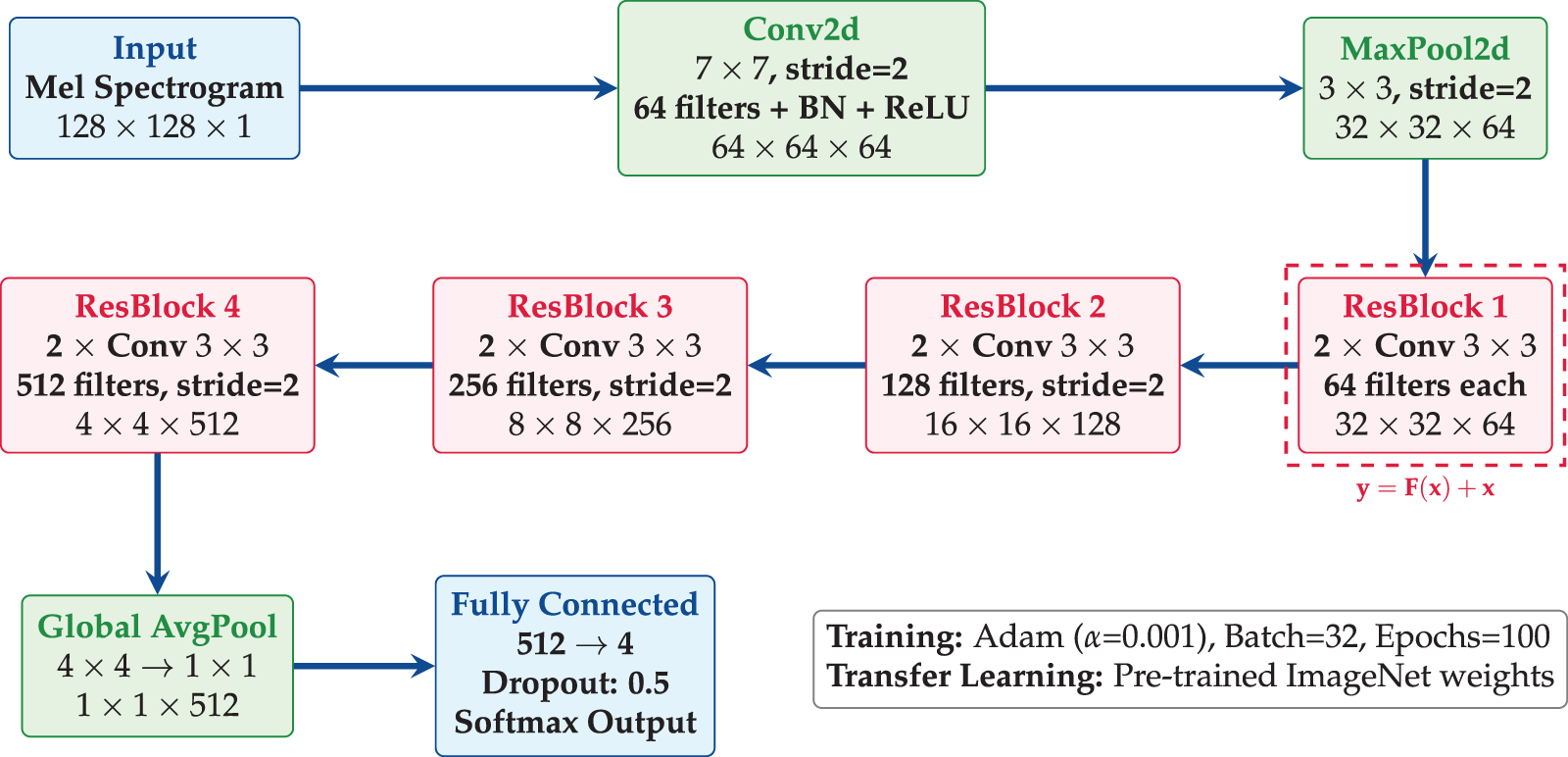
Figure 8: ResNet-18 architecture employs transfer learning with pre-trained ImageNet weights, and has four residual blocks with skip connections, global average pooling, and dropout regularization

•    Pre-trained Backbone: A ResNet-18 backbone is utilized for efficient feature extraction from spectrogram images. The ResNet architecture contains residual connections which are defined as:

y=F(x,{Wi})+x,(8)

where F represents the residual mapping and x is the input to the residual block. This allows the network to learn identity mappings, facilitating the training of deeper networks.

•    DataModule and LightningModule: The PyTorch model is organized into a DataModule for data handling and a LightningModule for model-related components such as model structure, loss computation, and optimization. The DataModule manages data loading, augmentation, and batching, while the LightningModule includes the model architecture and training logic.

•   Loss Function: The loss function that we used in this study is Cross-Entropy Loss, which is suitable for multi-class classification tasks. It is defined as:

ℒ(y,y^)=−∑i=1Kyilog⁡(y^i),(9)

where y is the actual label vector and y^ is the predicted vector.

•   Optimizer: The Adam optimizer is used to update the model parameters, with the following update rules:

mt=β1mt−1+(1−β1)gt,(10)

vt=β2vt−1+(1−β2)gt2,(11)

m^t=mt1−β1t,(12)

v^t=vt1−β2t,(13)

θt+1=θt−αm^tv^t+ϵ,(14)

where:

-   gt is the gradient of the loss with respect to the parameters at time step t.

-   mt and vt are the first and second moment estimates.

-   β1 and β2 are hyperparameters controlling the decay rates.

-   α is the learning rate.

-   ϵ is a small constant to prevent division by zero.

-   θt are the model parameters at time step t.

•   Training Loop: Handled by the Trainer class, the training loop includes callbacks for early stopping and model checkpoints, thus ensuring optimal model performance. The Trainer class also handles the training, validation, and testing phases, providing a streamlined interface for model experimentation.

The model is fine-tuned over 100 epochs with a batch size of 32. The use of a pre-trained ResNet-18 backbone allows the proposed model to benefit from features learned on a large dataset, improving its ability to generalize to new data.

3.6 Model Training and Optimization

The model’s training and optimization process was designed to maximize classification performance while preventing overfitting. Although using a pre-trained backbone accelerates convergence, the final accuracy is highly dependent on hyperparameter selection. Through a systematic search, the following optimal values were determined for our training configuration:

•   Learning Rate (α): A value of 0.001 was selected to balance convergence speed with training stability.

•   Batch Size: A batch size of 32 yielded the best results after experimentation with values ranging from 16 to 64.

•   Number of Epochs: The model was trained for a maximum of 100 epochs to ensure sufficient learning.

•   Optimizer Parameters: The standard parameters for the Adam optimizer were used: β1=0.9, β2=0.999, and ϵ=10−8.

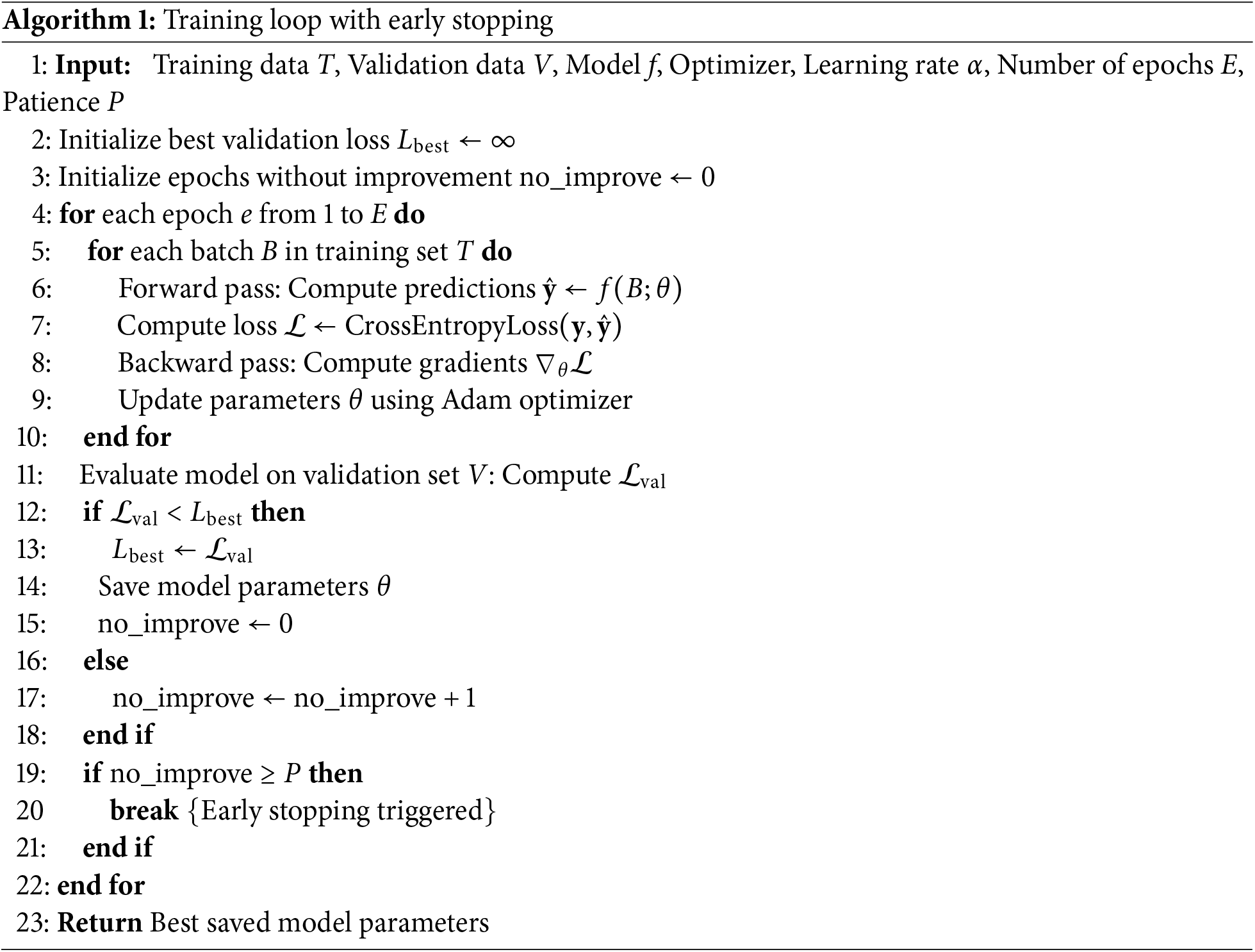
The training process involved iteratively updating the model parameters to minimize the cross-entropy loss on the training dataset using the Adam optimizer. To ensure the selection of the best-performing model and to mitigate overfitting, the training loop was enhanced with regularization techniques. Specifically, model checkpointing was used to save the model parameters that achieved the best performance on the validation set. Concurrently, an early stopping mechanism monitored the validation loss and halted training if no improvement was observed over a set number of consecutive epochs (the “patience” parameter). This combined approach ensures that the final model is not over-trained on the training data and generalizes well to unseen samples. The complete training procedure is formally detailed in Algorithm 1.

3.7 SNR-Based Classification Analysis

To assess the model’s robustness and simulate its performance in realistic clinical environments, we conducted a systematic analysis using signals contaminated with various types of noise at multiple Signal-to-Noise Ratio (SNR) levels.

3.7.1 Noise Simulation Protocol

Three distinct noise types were chosen to represent a spectrum of potential acoustic interference:

•   White Gaussian Noise: A standard benchmark representing broadband, spectrally flat, and uncorrelated noise.

•   Pink Noise: Characterized by a 1/f spectral density, this noise type more closely mimics many natural ambient sounds and physiological artifacts.

•   Ambient Hospital Noise: Authentic recordings from a clinical setting, providing the most ecologically valid condition by incorporating sounds like equipment beeps, distant conversations, and other real-world interference.

Each of these noise types was added to the clean, segmented PCG signals at four distinct SNR levels: 0, 10, 20, and 30. This range was selected to cover conditions from extremely noisy (0 dB) to minimally degraded (30 dB).

3.7.2 Experimental Setup

The noisy PCG signals for the evaluation were generated by superimposing a scaled noise signal onto each clean PCG segment according to the formula:

y[n]=x[n]+α⋅η[n],(15)

where y[n] is the resulting noisy signal, x[n] is the original segmented PCG signal, and η[n] is the noise signal. The scaling factor, α, was precisely calculated for each signal-noise pair to adjust the power of the noise component, thereby achieving the target SNR.

The CNN model, which was trained exclusively on the original clean dataset, was then evaluated on these newly generated noisy datasets. This experimental design allowed us to isolate and quantify the degradation in classification performance as a direct function of both noise type and intensity, providing a comprehensive measure of the model’s robustness to clinically relevant acoustic interference.

3.8 Benchmarking Model Architectures

To assess classification performance across different model complexities, four additional neural architectures were implemented. These models span from fully connected deep networks to transformer-based designs, each tailored for either handcrafted features (e.g., MFCCs) or time—frequency representations (e.g., Mel spectrograms).

3.8.1 Deep Neural Network (DNN)

A baseline fully connected model designed for low-dimensional feature vectors. The network consists of sequential linear layers (40→256→128→64→5) with ReLU activations and dropout (0.4) to prevent overfitting. This model serves as a lightweight reference without spatial priors.

3.8.2 Convolutional Neural Network (CNN)

A compact convolutional model optimized for spectrogram inputs. It includes three convolutional blocks (with 32, 64, and 128 filters), each followed by batch normalization, ReLU activation, and max pooling. The classifier employs global average pooling and fully connected layers to output five classes. This model balances accuracy with low computational cost, suitable for embedded or edge AI applications.

3.8.3 EfficientNet-B0

ImageNet-pretrained backbones were adapted for single-channel spectrograms by modifying the first convolutional layer to accept one input channel and replacing the final classification head with a five-class output layer. EfficientNet-B0 uses compound scaling to optimize depth, width, and resolution trade-offs, enhancing performance under limited PCG data.

3.8.4 Audio Spectrogram Transformer (AST)

A transformer-based model operating on spectrogram patches. The spectrogram is divided into non-overlapping 52×52 patches, each projected into a 512-dimensional embedding. These embeddings are processed through a multi-head self-attention encoder (8 heads, 10 layers) with positional encoding and a learnable class token. The transformer structure effectively captures global temporal–spectral dependencies, making it suitable for complex PCG signal analysis.

4  Results

4.1 Training and Validation Performance on the PhysioNet Dataset

The proposed model was trained for 100 epochs with a batch size of 32 on the PhysioNet 2016 dataset. The training concluded with a final accuracy of 96.2% on the training set and 94.1% on the validation set, demonstrating strong learning and generalization capabilities. To provide a more granular assessment of performance, we also computed the precision, recall, and F1-score for each class.

The confusion matrix, presented in Fig. 9, visualizes the model’s per-class classification accuracy. The strong diagonal concentration indicates a high true positive rate across all conditions, with minimal confusion between classes, confirming the model’s ability to effectively distinguish between the different cardiovascular pathologies in the dataset.

Figure 9: Confusion matrix for classification results. The matrix displays the performance on the validation set, with true labels on the y-axis and predicted labels on the x-axis. The values are normalized per class

4.2 Ablation Analysis

To quantify the contribution of key architectural components to the model’s performance, we conducted a comprehensive ablation study. Specific elements—such as regularization layers, network depth, and kernel size—were systematically removed or modified, and the resulting impact on performance was measured. The detailed outcomes of this analysis are presented in Table 2.

The results underscore the importance of each architectural choice. Removing dropout layers resulted in a 1.4% drop in accuracy, confirming their effectiveness in mitigating overfitting. The most significant performance degradation (a 2.6% drop) occurred upon removing batch normalization, highlighting its critical role in stabilizing the training process and improving generalization. Furthermore, reducing the model’s depth or using smaller kernel sizes also adversely affected performance, indicating that the baseline model’s complexity and receptive field are well-suited for capturing the hierarchical features present in the Mel spectrograms. As illustrated in Fig. 10, the baseline model consistently outperforms all ablated variants, underscoring the importance of each architectural component in achieving high classification accuracy.

Figure 10: The study evaluates the contribution of key architectural components such as dropout regularization, batch normalization, layer depth, and kernel size

4.3 Noise Robustness Analysis

To quantify the model’s resilience to acoustic interference, its performance was evaluated on datasets contaminated with various types of noise at different Signal-to-Noise Ratios (SNRs). The model, which was trained exclusively on clean data, demonstrated strong robustness at high SNRs, with only minor degradation in accuracy at 30 and 20 dB.

As detailed in Table 3, the performance decay becomes more pronounced at lower SNRs. The model maintains a respectable accuracy of 88.4% at a 10 dB SNR but experiences a significant drop to 75.1% in the most challenging 0 dB condition. These results highlight the inherent difficulty of classification in high-noise clinical environments and underscore the potential need for advanced denoising or data augmentation strategies to ensure reliability in real-world applications.

4.4 SNR-Based Classification Analysis

Fig. 11 illustrates the model’s classification accuracy as a function of both SNR level and noise type. The CNN model demonstrated robust performance under moderate noise, maintaining an accuracy above 90% for all noise types at SNR levels of 20 and 30 dB.

Figure 11: Classification accuracy across different SNR levels

As the noise level increased, performance began to degrade. At a 10 dB SNR, the model’s accuracy declined, averaging approximately 87% across the different noise conditions. This trend continued in the most challenging scenario (0 dB SNR), where the model’s accuracy fell below 80%, highlighting the significant difficulty of classification in extremely noisy environments. Overall, these results suggest that while the model can effectively handle moderate levels of noise interference, its reliability diminishes substantially under severe noise conditions.

4.5 Statistical Analysis

To validate the significance of the performance differences observed in the ablation study, we performed a statistical analysis using paired t-tests. These tests were conducted on the validation accuracy scores obtained from multiple independent training runs of the baseline model and each of its ablated variants.

Table 4 summarizes the results, comparing the mean accuracy of the baseline model against each variant. The calculated p-values confirm that the performance degradation observed upon removing key architectural components is statistically significant. The removal of batch normalization (p=0.01) and the reduction of network layers (p=0.001) resulted in highly significant decreases in model performance. This analysis provides quantitative evidence that each component of the proposed architecture plays a critical role in achieving the model’s overall high accuracy and robustness.

4.6 Performance and Efficiency Benchmarking

To evaluate our proposed ResNet-18 model, we benchmarked it against the architectures detailed in Section 3.8, including standard deep learning models (Deep Neural Network, Convolutional Neural Network) and state-of-the-art systems (EfficientNet-B0, Audio Spectrogram Transformer) as illustrated in Fig. 12. The goal of this analysis was to move beyond accuracy alone and to assess the critical trade-offs between diagnostic performance and the computational resources required for deployment, which is a central concern for hardware-aware AI and the development of practical medical devices.

Figure 12: Performance comparison of the proposed ResNet-18 with state-of-the-art methods. Statistical significance testing confirms improvements (p<0.001). Clinical validation on 2435 PCG recordings with robust performance under noise conditions

The results, as shown in Table 5, reveal a clear hierarchy in both performance and efficiency. At one extreme, the feature-based DNN, which operates on pre-extracted MFCCs, is by far the most computationally frugal model, with a negligible GFLOP count (0.00) and a tiny memory footprint (0.20 MB). However, this efficiency comes at the cost of significantly lower accuracy (84.4%). This demonstrates a classic trade-off: while expert feature engineering drastically reduces the computational load, it may not capture the full complexity of the signal, thereby limiting the model’s ultimate diagnostic capability.

At the other extreme, the Audio Spectrogram Transformer (AST) achieves the highest classification accuracy (96.9%). This underscores the power of large-scale, attention-based architectures for learning complex patterns from spectrogram data. However, this state-of-the-art performance is achieved at a substantial computational price. The AST is the largest model by a wide margin (85.47 MB) and has the second-highest computational cost (0.11 GFLOPs), making it less suitable for deployment on resource-constrained hardware or in real-time diagnostic scenarios.

Between these extremes lie the convolutional architectures. Our proposed ResNet-18 model strikes a highly effective and pragmatic balance. It delivers a classification accuracy (94.1%) that is only surpassed by the much larger AST, while significantly outperforming the simpler CNN and DNN baselines. While EfficientNet-B0 offers a smaller memory footprint, our ResNet-18 achieves a higher accuracy and precision. Most notably, the ResNet-18 architecture, despite its depth, has a GFLOP count of 0.57, which reflects a well-optimized balance between representational power and operational cost.

5  External Validation and Robustness Analysis on HLS-CMDS

To rigorously assess the generalizability and robustness of our deep learning approach, we conducted a series of experiments on the HLS-CMDS dataset, which was entirely unseen during the initial training on the PhysioNet dataset. These experiments were designed to answer critical questions about model adaptation, domain shift, and sensitivity to signal processing artifacts. However, it should be noted that HLS-CMDS serves solely for adaptation testing, not as a substitute for real-world models. We emphasize that PhysioNet-trained models remain foundational, with manikin validation highlighting domain shifts.

5.1 Experiment 1: Fine-Tuning for Binary Classification

First, we evaluated the direct transferability of the PhysioNet-trained model by adapting it for a binary (Normal vs. Abnormal) classification task on the HLS-CMDS dataset. After fine-tuning the final layer for 10 epochs with a low learning rate, the model achieved a test accuracy of 88.0%.

As detailed in Table 6, the model demonstrated excellent performance in identifying ‘Abnormal’ sounds (F1-score of 0.92) but was less effective with ‘Normal’ sounds (F1-score of 0.71). The confusion matrix is shown in Fig. 13. This performance imbalance suggests that while the features learned on PhysioNet are effective for recognizing general pathologies, they may also carry a bias that leads to the misclassification of normal variations present in the new dataset.

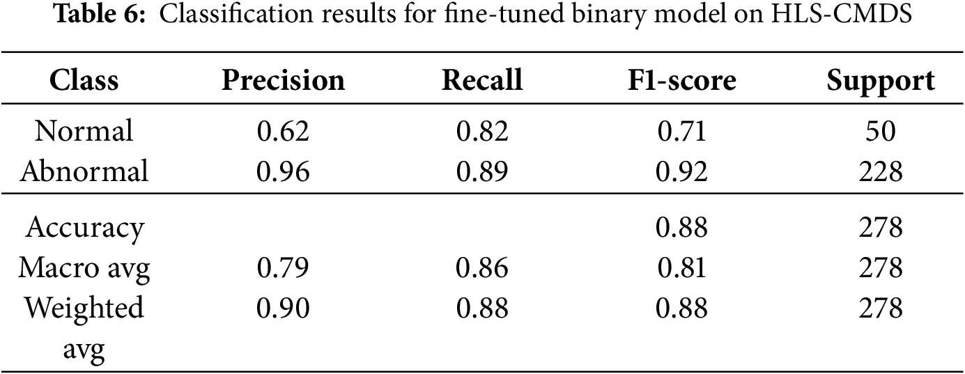
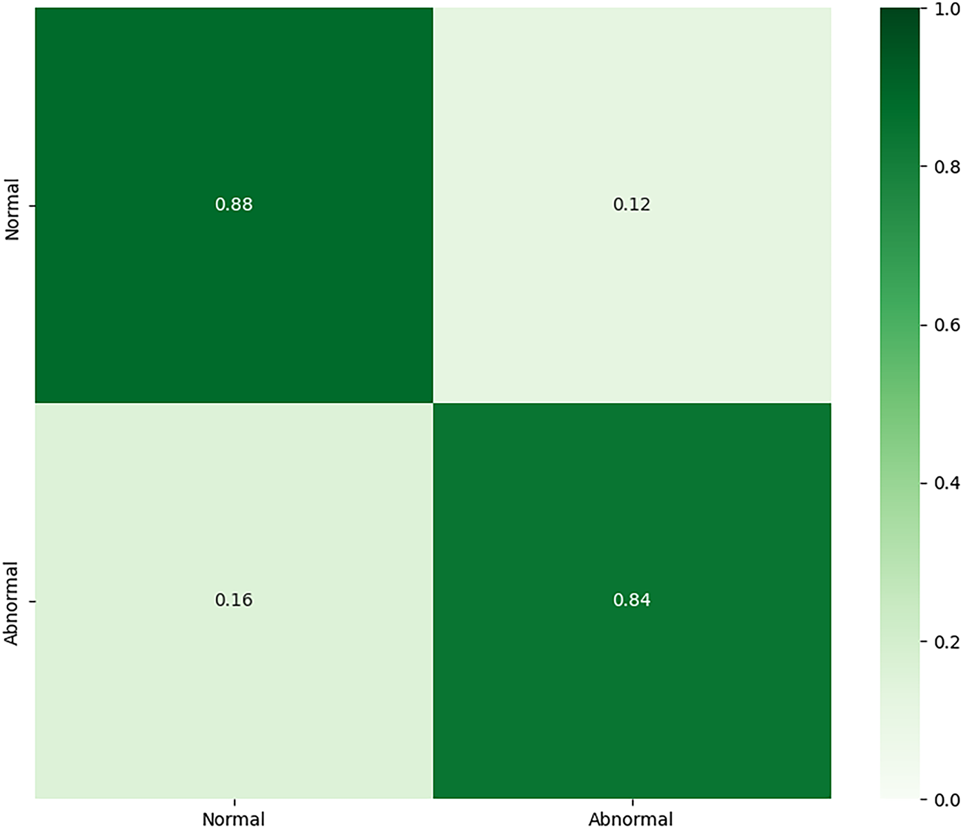
Figure 13: Confusion matrix for the fine-tuned binary classification model on the HLS-CMDS test set

5.2 Experiment 2: Fine-Tuning for Multi-Class Classification

Next, we adapted the PhysioNet-trained model for a more granular four-class problem: ‘Normal’, ‘Murmur’, ‘Extra Sound’, and ‘Rhythm Disorder’. The fine-tuned model achieved a test accuracy of 86.0%. As shown in Table 7, while it performed strongly on the well-represented ‘Murmur’ class (F1-score of 0.91), its performance was notably lower for ‘Extra Sound’ and ‘Rhythm Disorder’. The confusion matrix for Experiment 2 is illustrated in Fig. 14. This suggests that the features transferred from the source dataset are less effective at distinguishing between specific, novel pathologies, particularly for classes with fewer samples.

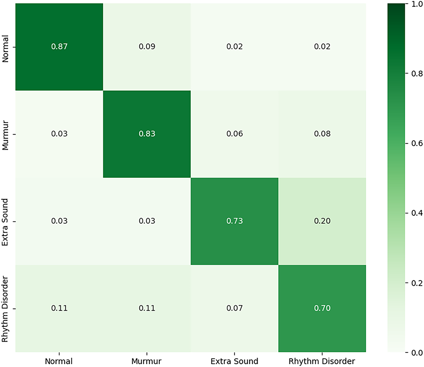
Figure 14: Confusion matrix for the fine-tuned multi-class model on the HLS-CMDS test set

5.3 Experiment 3: Full Retraining on HLS-CMDS Dataset

To determine if domain-specific training could outperform fine-tuning, we initialized a new ResNet-18 model with standard ImageNet weights and retrained it from scratch on the four-class HLS-CMDS data. This approach yielded a higher test accuracy of 89.0%. As detailed in Table 8, the retrained model showed more balanced performance across all classes, notably improving the F1-score for ‘Rhythm Disorder’. However, we observe that the minority classes, such as ‘Extra Sound’ (n = 37), still exhibit lower precision, indicating that class imbalance remains a challenge. Nonetheless, these results suggest that for a sufficiently diverse target dataset, allowing the model to learn domain-specific features directly can be more effective than transferring potentially biased features from another medical dataset. The confusion matrix is shown in Fig. 15.

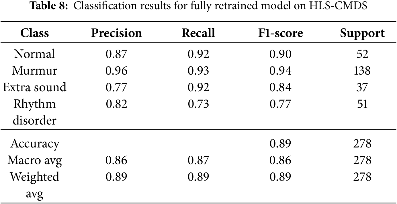
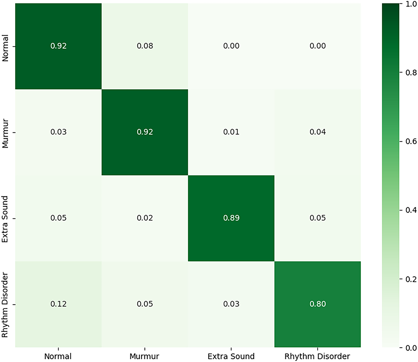
Figure 15: Confusion matrix for the fully retrained model on the HLS-CMDS test set

5.4 Experiment 4: Robustness to Signal Separation Artifacts

Finally, we designed a novel stress test to assess the model’s robustness to artifacts introduced by upstream signal processing. The model from Experiment 3 (retrained on clean HLS-CMDS data) was evaluated on a test set of heart sounds that had been computationally separated from mixed heart-lung recordings using a bandpass filter.

The results, shown in Table 9, reveal a catastrophic drop in performance to an accuracy of just 41.0%. The model struggled to identify any class reliably, with F1-scores collapsing across the board, as illustrated in Fig. 16. This critical finding demonstrates that the model, while robust to additive environmental noise, is extremely brittle when faced with the subtle distortions and information loss introduced by the signal separation process. This exposes a significant challenge for real-world deployment, where such preprocessing algorithms are common, and highlights that a model’s robustness must be evaluated against the entire processing pipeline, not just environmental noise.

Figure 16: Confusion matrix for the retrained model evaluated on computationally separated heart sounds

6  Discussion

Our study provides several critical insights into the practical deployment of deep learning models for heart sound classification. The initial results on the PhysioNet dataset established a strong performance baseline, while the subsequent experiments on the HLS-CMDS dataset were designed to probe the real-world challenges of generalizability, domain shift, and robustness to signal processing artifacts. This comprehensive analysis moves beyond single-dataset performance metrics to offer a more nuanced understanding of the model’s strengths and weaknesses.

6.1 Generalizability and the Fine-Tuning vs. Retraining Trade-off

The external validation on the HLS-CMDS dataset yielded several important findings regarding model adaptation. The fine-tuning experiments (Experiments 1 and 2) demonstrated that a model pre-trained on a large PCG dataset (PhysioNet) can generalize reasonably well to a new, unseen dataset, achieving 88% and 86% accuracy for binary and multi-class tasks, respectively. This confirms the value of transfer learning within the PCG domain. However, the model’s high recall for ‘Abnormal’ sounds, paired with lower precision for ‘Normal’ sounds, indicates a potential bias learned from the source dataset, causing the model to be overly sensitive to variations in the new data.

Interestingly, Experiment 3 showed that retraining a ResNet-18 model with generalist ImageNet weights directly on the HLS-CMDS data yielded superior and more balanced performance (89% accuracy). This suggests a key trade-off: while domain-specific pre-training is beneficial, it may also introduce biases that hinder adaptation to a new dataset with different characteristics, such as those originating from a clinical manikin instead of human subjects. When the target dataset is sufficiently diverse, allowing the model to learn features from a more general starting point like ImageNet can be a more effective strategy. This approach avoids inheriting the specific biases of the source medical dataset and can lead to better performance, although challenges related to class imbalance in the target data may still persist, as seen in the lower precision for minority classes like ‘Extra Sound’.

6.2 Robustness: Environmental Noise vs. Processing Artifacts

A primary contribution of this work is the dual analysis of model robustness. The initial SNR-based analysis confirmed that the model is highly resilient to additive environmental noise, maintaining over 90% accuracy even at a 20 dB SNR. This is a crucial feature for clinical viability, where background noise is unavoidable.

However, Experiment 4 exposed a critical vulnerability. The dramatic collapse in performance from 89% on clean HLS-CMDS data to a mere 41% on computationally separated heart sounds is a stark reminder of the ‘brittleness’ of deep learning models. The model, while robust to environmental noise, was extremely sensitive to the subtle distortions and potential information loss introduced by the standard bandpass filter used for source separation. This finding highlights a critical, often-overlooked challenge: a model’s performance is not just a function of its architecture and training data but is also deeply coupled to the specific preprocessing pipeline used. The inherent limitation of a simple filter to perfectly separate spectrally overlapping signals means that any such imperfection in a real-world pipeline could lead to catastrophic failure. This strongly suggests that future research must prioritize robustness not only to environmental noise but also to variations and artifacts from upstream signal processing components.

6.3 The Importance of Model Architecture and Regularization

Our ablation studies, conducted on the PhysioNet dataset, underscore the importance of deliberate architectural choices. The removal of dropout layers led to a 1.4% drop in accuracy, confirming its role in preventing overfitting by forcing the network to learn more robust representations. The most significant performance decrease (2.6%) was observed upon removing batch normalization, which highlights its dual role in stabilizing the training process and providing a regularizing effect essential for generalization. Furthermore, reducing the model’s depth resulted in a substantial performance drop, confirming that a deep architecture is necessary to learn the hierarchical features present in Mel spectrograms. These results provide a strong empirical justification for the architectural design, emphasizing that each component plays a critical role in achieving high performance.

6.4 Limitations and Future Directions

This study, while comprehensive, has several limitations that provide clear avenues for future work:

•   The segmentation of the PhysioNet dataset was dependent on concurrent ECG recordings. This highlights the direct consequence of our methodological choice to focus on the systolic window, a common simplification that is effective for certain pathologies but, as our experiments on the HLS-CMDS dataset demonstrated, makes the model incapable of identifying conditions defined by diastolic events, such as the ‘Extra Sound’ class.

•   The signal separation in Experiment 4 was performed with a standard bandpass filter. As noted, this method is imperfect due to the spectral overlap between heart and lung sounds. More advanced source separation algorithms based on deep learning or independent component analysis should be explored to determine if they produce artifacts to which the model is more robust.

•   While the HLS-CMDS dataset provides a controlled and repeatable environment for external validation, data from a clinical manikin does not capture the full biological variability of a human population. Final clinical validation must be performed on extensive, real-world patient data.

Our findings also suggest a clear need for a new direction in data augmentation. To build truly robust models, training data should be augmented not only with environmental noise but also with signals that have undergone various forms of processing (e.g., different filtering, compression, or separation algorithms). This ‘processing-aware’ augmentation could train models to be robust to the entire end-to-end clinical pipeline. Finally, the success of retraining on HLS-CMDS suggests that developing foundational models on massive, diverse PCG datasets from multiple sources is a promising path toward truly generalizable heart sound classifiers that require minimal fine-tuning for new clinical environments.

7  Conclusion

This study developed and rigorously validated a deep learning framework for PCG signal classification, demonstrating both the potential and the practical challenges of deploying such models in clinical settings. Our work confirms that CNNs can achieve high accuracy on benchmark datasets and can be successfully adapted to new domains through fine-tuning or retraining. However, our most critical contribution is the exposure of a significant vulnerability: while the model is robust to additive environmental noise, its performance collapses when faced with artifacts from upstream signal processing, a finding with major implications for real-world deployment.

Despite the strong baseline performance, this study has several limitations. The initial model’s reliance on concurrent ECG signals for segmentation restricts its applicability in scenarios where only PCG is available. Furthermore, the external validation was conducted on data from a clinical manikin, which, while providing a controlled environment, does not fully capture the biological variability of human subjects. Most importantly, our stress test revealed that the model’s performance is tightly coupled to the specific preprocessing pipeline, highlighting a critical point of failure.

Future work must prioritize addressing these challenges. Key endeavors should include the development of robust, ECG-free segmentation algorithms and the design of models that are inherently resilient to processing artifacts, potentially through ‘processing-aware’ data augmentation. Ultimately, extensive clinical validation on large-scale, multi-source patient datasets will be essential for building truly generalizable classifiers. The insights gained from this study lay a strong foundation for the continued advancement of automated cardiovascular diagnostics, contributing to improved patient outcomes and the broader field of medical machine learning.

Acknowledgement: The researchers would like to thank the Deanship of Graduate Studies and Scientific Research at Qassim University for financial support (QU-APC-2025).

Funding Statement: This work was funded by the Deanship of Graduate Studies and Scientific Research at Qassim University through grant number (QU-APC-2025).

Author Contributions: The authors confirm their contributions to the paper as follows: Conceptualization: Akbare Yaqub, Muhammad Sadiq Orakzai, Muhammad Farrukh Qureshi; Methodology: Akbare Yaqub, Muhammad Farrukh Qureshi; Software: Akbare Yaqub, Muhammad Farrukh Qureshi; Validation: Akbare Yaqub, Muhammad Sadiq Orakzai, Muhammad Farrukh Qureshi; Formal analysis: Akbare Yaqub; Investigation: Akbare Yaqub; Resources: Muhammad Sadiq Orakzai, Muhammad Farrukh Qureshi; Data curation: Akbare Yaqub; Writing—original draft preparation: Akbare Yaqub; Writing—review and editing: Akbare Yaqub, Muhammad Sadiq Orakzai, Muhammad Farrukh Qureshi, Zohaib Mushtaq, Imran Siddique, Taha Radwan; Visualization: Akbare Yaqub, Muhammad Farrukh Qureshi; Supervision: Muhammad Sadiq Orakzai, Muhammad Farrukh Qureshi; Project administration: Zohaib Mushtaq, Imran Siddique, Taha Radwan; Funding acquisition: Imran Siddique, Taha Radwan. All authors reviewed the results and approved the final version of the manuscript.

Availability of Data and Materials: The dataset analysed during the current study is available in the PhysioNet Challenge2016 repository, https://www.kaggle.com/datasets/bjoernjostein/physionet-challenge-2016 (accessed on 26 October 2025).

Ethics Approval: Not applicable.

Conflicts of Interest: The authors declare no conflicts of interest to report regarding the present study.

References

1. Gaziano TA. Cardiovascular diseases worldwide. Public Health Approach Cardiovasc Dis Prev Manag. 2022;1:8–18. [Google Scholar]

2. Baghdadi NA, Farghaly Abdelaliem SM, Malki A, Gad I, Ewis A, Atlam E. Advanced machine learning techniques for cardiovascular disease early detection and diagnosis. J Big Data. 2023;10(1):144. doi:10.1186/s40537-023-00817-1. [Google Scholar] [CrossRef]

3. Bridge P, Fielding A, Rowntree P, Pullar A. Intraobserver variability: should we worry? J Med Imaging Radiat Sci. 2016;47(3):217–20. doi:10.1016/j.jmir.2016.06.004. [Google Scholar] [PubMed] [CrossRef]

4. Wong KK, Fortino G, Abbott D. Deep learning-based cardiovascular image diagnosis: a promising challenge. Future Gener Comput Syst. 2020;110:802–11. doi:10.1016/j.future.2019.09.047. [Google Scholar] [CrossRef]

5. Tayyeb M, Umer M, Alnowaiser K, Sadiq S, Majeed R, Abdullah M, et al. Deep learning approach for automatic cardiovascular disease prediction employing ECG signals. Comput Model Eng Sci. 2023;137(2):1677. [Google Scholar]

6. Rojas MR, Rivet B, Kavouni NM, Fontecave-Jallon J. Phonocardiography for robust fetal heart rate estimation in real clinical conditions. Biomed Signal Process Control. 2025;107(1):107807. doi:10.1016/j.bspc.2025.107807. [Google Scholar] [CrossRef]

7. Ghosh SK, Ponnalagu R, Tripathy RK, Panda G, Pachori RB. Automated heart sound activity detection from PCG signal using time-frequency-domain deep neural network. IEEE Trans Instrum Meas. 2022;71(2):1–10. doi:10.1109/tim.2022.3192257. [Google Scholar] [CrossRef]

8. Patwa A, Mahboob Ur Rahman M, Al-Naffouri TY. Heart murmur and abnormal PCG Detection via wavelet scattering transform and 1D-CNN. IEEE Sens J. 2025;25(7):12430–43. doi:10.1109/jsen.2025.3541320. [Google Scholar] [CrossRef]

9. Marnani RA, Jaros R, Pavlicek J, Martinek R, Kahankova RV. Advancements and challenges in non-invasive electrocardiography for prenatal, intrapartum, and postnatal care: a comprehensive review. IEEE Access. 2024;12(7):44730–47. doi:10.1109/access.2024.3378747. [Google Scholar] [CrossRef]

10. Abbasi SF, Abbas A, Ahmad I, Alshehri MS, Almakdi S, Ghadi YY, et al. Automatic neonatal sleep stage classification: a comparative study. Heliyon. 2023;9(11):e22195. doi:10.1016/j.heliyon.2023.e22195. [Google Scholar] [PubMed] [CrossRef]

11. Siddiqa HA, Qureshi MF, Khurshid A, Xu Y, Wang L, Abbasi SF, et al. EEG electrode setup optimization using feature extraction techniques for neonatal sleep state classification. Front Comput Neurosci. 2025;19:1506869. doi:10.3389/fncom.2025.1506869. [Google Scholar] [PubMed] [CrossRef]

12. Sugiyarto AW, Abadi AM, Sumarna S. Classification of heart disease based on PCG signal using CNN. TELKOMNIKA (Telecommun Comput Elec Control). 2021;19(5):1697–706. doi:10.12928/telkomnika.v19i5.20486. [Google Scholar] [CrossRef]

13. Baghel N, Dutta MK, Burget R. Automatic diagnosis of multiple cardiac diseases from PCG signals using convolutional neural network. Comput Methods Programs Biomed. 2020;197(12):105750. doi:10.1016/j.cmpb.2020.105750. [Google Scholar] [PubMed] [CrossRef]

14. Qamar HGM, Qureshi MF, Mushtaq Z, Zubariah Z, ur Rehman MZ, Samee NA, et al. EMG gesture signal analysis towards diagnosis of upper limb using dual-pathway convolutional neural network. Math Biosci Eng. 2024;21(4):5712–34. doi:10.3934/mbe.2024252. [Google Scholar] [PubMed] [CrossRef]

15. Qureshi MF, Mushtaq Z, Ur Rehman MZ, Kamavuako EN. Spectral image-based multiday surface electromyography classification of hand motions using CNN for human-computer interaction. IEEE Sens J. 2022;22(21):20676–83. doi:10.1109/jsen.2022.3204121. [Google Scholar] [CrossRef]

16. Qureshi MF, Mushtaq Z, Rehman MZU, Kamavuako EN. E2CNN: an efficient concatenated CNN for classification of surface EMG extracted from upper limb. IEEE Sens J. 2023;23(8):8989–96. doi:10.1109/jsen.2023.3255408. [Google Scholar] [CrossRef]

17. Hangaragi S, Neelima N, Jegdic K, Nagarwal A. Integrated fusion approach for multi-class heart disease classification through ECG and PCG signals with deep hybrid neural networks. Sci Rep. 2025;15(1):8129. doi:10.1038/s41598-025-92395-w. [Google Scholar] [PubMed] [CrossRef]

18. Chowdhury MTH, Poudel KN, Hu Y. Time-frequency analysis, denoising, compression, segmentation, and classification of PCG signals. IEEE Access. 2020;8:160882–90. doi:10.1109/access.2020.3020806. [Google Scholar] [CrossRef]

19. Marzorati D, Dorizza A, Bovio D, Salito C, Mainardi L, Cerveri P. Hybrid convolutional networks for end-to-end event detection in concurrent PPG and PCG signals affected by motion artifacts. IEEE Trans Biomed Eng. 2022;69(8):2512–23. doi:10.1109/tbme.2022.3148171. [Google Scholar] [PubMed] [CrossRef]

20. Ghosh SK, Ponnalagu RN, Tripathy RK, Acharya UR. Automated detection of heart valve diseases using chirplet transform and multiclass composite classifier with PCG signals. Comput Biol Med. 2020;116(5):103543. doi:10.1016/j.compbiomed.2020.103632. [Google Scholar] [PubMed] [CrossRef]

21. Altaf A, Mahdin H, Mahmood A. Systematic review for phonocardiography classification based on machine learning. Int J Adv Comput Sci Appl. 2023;14(8):8. doi:10.14569/ijacsa.2023.0140889. [Google Scholar] [CrossRef]

22. Li F, Tang H, Shang S, Mathiak K, Cong F. Classification of heart sounds using convolutional neural network. Appl Sci. 2020;10(11):3956. doi:10.3390/app10113956. [Google Scholar] [CrossRef]

23. Tang H, Dai Z, Jiang Y, Li T, Liu C. PCG classification using multidomain features and SVM classifier. Biomed Res Int. 2018;2018(1):4205027. doi:10.1155/2018/4205027. [Google Scholar] [PubMed] [CrossRef]

24. Dominguez-Morales JP, Jimenez-Fernandez AF, Dominguez-Morales MJ, Jimenez-Moreno G. Deep neural networks for the recognition and classification of heart murmurs using neuromorphic auditory sensors. IEEE Trans Biomed Circuits Syst. 2018;12(1):24–34. doi:10.1109/tbcas.2017.2751545. [Google Scholar] [PubMed] [CrossRef]

25. Sotaquirá M, Alvear D, Mondragón M. Phonocardiogram classification using deep neural networks and weighted probability comparisons. J Med Eng Technol. 2018;42(7):510–7. [Google Scholar] [PubMed]

26. Khan KN, Khan FA, Abid A, Olmez T. Deep learning based classification of unsegmented phonocardiogram spectrograms leveraging transfer learning. Physiol Meas. 2021;42(9):9. doi:10.1088/1361-6579/ac1d59. [Google Scholar] [PubMed] [CrossRef]

27. Krishnan PT, Balasubramanian P. Automated heart sound classification system from unsegmented phonocardiogram (PCG) using deep neural network. Phys Eng Sci Med. 2020;43(2):505–15. doi:10.1007/s13246-020-00851-w. [Google Scholar] [PubMed] [CrossRef]

28. Chen W, Sun Q, Chen X, Xie G, Wu H, Xu C. Deep learning methods for heart sounds classification: a systematic review. Entropy. 2021;23(6):667. doi:10.3390/e23060667. [Google Scholar] [PubMed] [CrossRef]

29. Milani MGM, Abas PE, Silva LCD, Nanayakkara ND. Abnormal heart sound classification using phonocardiography signals. Smart Health. 2021;21(11):100194. doi:10.1016/j.smhl.2021.100194. [Google Scholar] [CrossRef]

30. Arora V, Leekha R, Singh R, Chana I. Heart sound classification using machine learning and phonocardiogram. Mod Phys Lett B. 2019;33(26):1950321. doi:10.1142/s0217984919503214. [Google Scholar] [CrossRef]

31. Liu C, Springer D, Li Q, Moody B, Juan RA, Chorro FJ, et al. An open access database for the evaluation of heart sound algorithms. Physiol Meas. 2016;37(12):2181–213. [Google Scholar] [PubMed]

32. Torabi Y, Shirani S, Reilly JP. Descriptor: heart and lung sounds dataset recorded from a clinical manikin using digital stethoscope (HLS-CMDS). IEEE Data Des. 2025;2(3):133–40. doi:10.1109/ieeedata.2025.3566012. [Google Scholar] [CrossRef]

33. Liu Q, Wu X, Ma X. An automatic segmentation method for heart sounds. Biomed Eng Online. 2018;17(1):106. [Google Scholar] [PubMed]

34. Park C, Shin K, Seo J, Lim H, Kim GH, Seo WY, et al. Enhancement of phonocardiogram segmentation using convolutional neural networks with Fourier transform module. Biomed Eng Lett. 2025;15(2):401–13. doi:10.1007/s13534-025-00458-8. [Google Scholar] [PubMed] [CrossRef]

35. Alquran H, Al-Issa Y, Alsalatie M, Tawalbeh S. Deep learning models for segmenting phonocardiogram signals: a comparative study. PLoS One. 2025;20(4):e0320297. doi:10.1371/journal.pone.0320297. [Google Scholar] [PubMed] [CrossRef]