Predicting Concrete Strength Using Data Augmentation Coupled with Multiple Optimizers in Feedforward Neural Networks

1  Introduction

Concrete is the most widely utilized construction material, crucially essential for infrastructure development and building construction. The components of concrete are cement, aggregates (sand and gravel), and water, which make it strong, durable, and versatile. The aggregates are joined together by the cement paste, resulting in a solid, long-lasting material with improved qualities. Still, the manufacturing and use of concrete have substantial environmental, financial, and resource concerns [1,2]. The annual consumption of natural aggregates (NAs) for concrete production is estimated at 8–12 billion tons globally [3]. NAs in concrete manufacturing, either as gravel or sand, have certain environmental drawbacks like habitat destruction, water pollution, resource depletion, CO2 emissions, and land use. The construction industry in the United Kingdom supplies about 44% of landfill waste, while in Australia the industry’s land waste is approximately 44%, 29% in the United States, and 35% across the globe [4]. China, on average, generates 8 billion tons of construction and demolition waste (CDW) every year [5]. Nonetheless, it is undeniable that construction and demolition debris is notorious for its detrimental impact on the environment [6]. CDW remains are generally classified into five categories, i.e., unsorted mixed fractions, wood, metal, concrete, and minerals [7]. Concrete waste constitutes the largest proportion of construction waste, comprising approximately 35% of the grand [8]. One of the biggest polluters, the construction sector, is beginning to show concern for the problem [9]. Also, in recent years, there has been an increasing interest in discovering sustainable alternatives to construction materials [10]. CDW can be used as aggregates in recycled aggregate (RA) form as a substitute for natural resources in concrete mixes. It could be one way to lessen the environmental impact. Also, this enhances performance and conform to sustainable construction principles, rendering them essential for future advancements in the sector [11]. Numerous academics have investigated methods for producing concrete with recycled aggregates (RAs), which recommends that more than 75% of construction debris might be recycled to produce concrete, mainly to lower CO2 emissions [5].

Many researchers are focusing on predicting various properties of concrete with different components. Numerous concrete attributes, covering mechanical, thermal, and durability aspects, have been predicted in-depth in the literature, and the effectiveness of several prediction techniques has been studied and documented [12,13]. The compressive strength (CS) of concrete, being the most crucial property, has been the foremost priority of researchers to predict, as concrete made with recycled aggregates (RAs) exhibits complex relationships between design mix components and CS, and traditional methods of concrete mix design are material, cost, labor, and time intensive [10]. The manual testing procedure is susceptible to human error as well, and even minor mistakes may significantly extend the typical wait time [14]. Since RAC is mixed with different types of recycled materials, it is hard to accurately forecast its performance using conventional regression strategies [15]. The poor qualities of RAs, such as higher affinity for water, higher brittleness of the old mortar, cracks created during the crushing process, and weak bonding between old and new mortar, are the main reasons for the unpredictable behavior of concrete having recycled aggregates [16]. Concrete manufactured using RAs has a 30% to 40% lower CS than natural aggregate concrete (NAC) due to the inferior qualities of recycled particles [17,18]. In the civil engineering discipline, the development and application of machine learning (ML) techniques have garnered significant interest recently [19]. These techniques have primarily been used for optimization and prediction [20]. Recent ML model-based studies on experimental data can anticipate the influence of CDW aggregate in the concrete behavior with an acceptable error range, improving one-factor-at-a-time experimental method studies by lowering the amount of materials used, testing efforts, time consumed, and cost incurred [21]. Furthermore, a key benefit of using ML approaches is their ability to consider a multitude of input factors [22], and ML encompasses a wide variety of algorithms that can grasp patterns in data [23]. These models have demonstrated significant efficacy in recreating both experimental and numerical simulations, while minimizing the time and computational expenses typically linked to conventional methods [24]. The most popular artificial intelligence approach for assessing the CS of various concrete families is ANN [25].

Numerous researchers have considered multiple input factors while using ML algorithms for the prediction of the CS of concrete. Xu et al. [26] have only considered water-to-cement ratio, maximum aggregate size, and aggregate-to-cement ratio as influencing factors for the prediction of CS of concrete using multiple nonlinear regression (MNLR) and artificial neural network (ANN). Dantas et al. [21] examined several input variables in the prediction of CS of recycled aggregate concrete (RAC) using artificial neural networks (ANNs): water to cement ratios, cement content, dry mortar ratio, total dry aggregate concrete, the aggregate substitution ratio of recycled fine aggregates and coarse aggregates, chemical admixture rate, composition of CDW, ratio of recycled mortar and concrete, ratio of recycled materials, fineness modulus of natural and recycled fine aggregates and coarse aggregates, maximum aggregate size of fine aggregates and coarse aggregates, water absorption rates of recycled fine aggregates (RFA) and coarse aggregates (RCA), and the compensation rates of water absorption. The analysis also incorporates the age of the concrete. Overall cement content, sand content and recycled coarse aggregates. Water content, w/c%, and substitution ratio of RCA were the factors studied as input variables by Hu et al. [5]. The fineness modulus, densities, particle sizes of coarse and natural aggregates, and age are other parameters infrequently employed by some researchers [25].

Many material designers and researchers employ ANNs as the approximation method for forecasting various properties of construction materials. Allegedly, ANNs mimic the learning patterns of human brains by repeating actions in different contexts and replicate these patterns to make decisions in unforeseen situations [27]. ANNs employ a learning process that assigns random values (weights) to each unit, known as a neuron, to assess the impact of input data on the prediction of an output. After acquiring and examining a signal, these artificial neurons transmit information to the next consecutive neurons connected to it. Non-linear functions produce each output by aggregating their inputs, with the “signal” at a connection represented as a real number. Links are referred to as edges [25]. As learning advances, the relative weights of neurons and edges are updated until the best solution—one with the minimum mean-squared error (MSE) is found. Other evaluation parameters most frequently used are coefficient of determination (R2), mean absolute error (MAE) or mean absolute percentage error (MAPE), and root mean square error (RMSE) for validation of the performance of the model [25]. A more accurate model reveals lower values of RMSE, MAE, and MSE but with a larger R2 indicates enhanced accuracy. The training of the ANNs is a nondeterministic process because, primarily as a result of this unpredictability in the coefficient generation, the ANNs tend to converge to one local minima/maxima from a pool of potential solutions [28]. The most crucial hyperparameters in ANN models are frequently the starting weights, learning rate, number of epochs/iterations, activation functions, number of layers, and number of neurons [29]. Different activation functions like sigmoid, hyperbolic tangent (Tanh), rectified linear unit (ReLU), leaky ReLU, exponential linear unit (ELU) are available in literature. It is apparent from literature that the sigmoid function was utilized as an activation function by the majority of researchers and material designers [30]. A feed-forward neural net (FFNN) is an architecture, in which each layer is simply coupled to its immediate neighbor layers, is the most basic architecture that an ANN model may adopt. As a result, serial and linear mapping is accomplished from the input to the output layers through the hidden layers [27]. Feedforward neural networks (FFNNs) are easier to understand than more complex neural architectures due to their simple structure, and their training process is typically straightforward and efficient. Numerous studies have demonstrated the efficacy of FFNNs, particularly in material modeling [22]. Reference [31] used ANNs to predict the concrete CS having RAs with one hidden layer and 14 input variables and model generated represents fairly high accuracy. Reference [32] forecasted the CS of RAC using a nonlinear, regression-based ML model, namely an ANN. In order to forecast the mechanical properties of RAC, reference [33] examined the suitability of a number of regression-based ML models, including least squares support vector regression (LSSVR) models, M5 model tree (M5Tree), and multivariate adaptive regression splines (MARS). CS of RAC using a convolutional ANN-based deep learning algorithm was predicted by [34]. ANNs and response surface methodology (RSM) have been used by [35] to estimate the concrete compressive strength having RAs and the outputs of these models were assessed, which revealed that the precision of ANNs is better than RSM. ANN is the most often used ML model [36], and it is anticipated that the precision of ML approaches will increase with the number of input variables and data points [36].

Compiling huge datasets from the literature is a hectic and tedious task. ML models demand big and premium quality datasets. Overfitting issues are common in models trained on datasets with fewer than 1000 data points [37]. Models trained on fewer than 1000 data points are particularly prone to overfitting issues [37]. According to [38], only 11% of studies applying ML to concrete science utilize datasets exceeding 1000 samples. To mitigate data scarcity in predicting concrete mix design properties, researchers have increasingly turned to generative approaches. For instance, generative adversarial networks (GANs) have been employed to generate synthetic data for the CS of concrete incorporating industrial waste materials [39]. Conditional GANs (CGANs), cycle-consistent deep GANs (CDGANs) [40], and tabular GANs (TGANs) [41,42] have been used to simulate data for ultra-high-performance concrete. Similarly, reference [38] applied TGANs to generate synthetic datasets for predicting the CS of geopolymer concrete.

Hence, this study presents a novel approach by simultaneously utilizing five different in-built optimizers in MATLAB Neural Net fitting module for the development of an ANN model, specifically focusing on feedforward neural networks (FFNN) due to their simplicity, ease of implementation, and time efficiency. By utilizing multiple optimizers, the study aims to enhance the performance and robustness of model. Random forest (RF) and extreme gradient (XGBoost) models were also trained and evaluated. RF functions as a bagging technique that mitigates variance by concurrently training multiple decision trees on various bootstrapped samples and averaging their outcomes. While XGBoost employs a boosting approach, constructing trees in a sequential manner where each subsequent tree aims to reduce the errors made by its predecessors, thereby minimizing bias and improving accuracy. NNs, however, differ logically from both methods, as it function as a singular, robust model that learns intricate, hierarchical patterns directly from the data by modifying interconnected layers of neurons through the process of backpropagation. Additionally, the incorporation of advanced interpolation-based data augmentation techniques allows the model to achieve high accuracy with a relatively smaller dataset collected from literature, illustrating the efficacy of techniques in refining model generalization and performance. This dual strategy of optimizer diversity and data augmentation represents a significant advancement in FFNN model development. Next, models developed utilizing synthetic data have been compared with models using original data with evaluation metrics such as R-squared (R2), correlation coefficient (R), mean absolute error (MAE), mean absolute percentage error (MAPE), root mean squared error (RMSE) and mean squared error (MSE). Additionally, sensitivity analysis employing perturbation and weight-partitioning techniques was carried out to enhance understanding of the performance of model and to assess the relative importance of the input parameters. To further elucidate the influence of these variables on model output and predictions, partial dependence plots (PDP) and accumulated local effects (ALE) were incorporated, offering deeper interpretability of feature impacts.

1.1 Artificial Neural Network and Training Algorithms

ANNs are designed mathematical frameworks that imitate the neural biological systems identical human brain, enabling them to learn and solve problems. An ANN can be conceived of as a mesh of several processors called units or neurons [43]. Structure and function of a neuron or node—the fundamental building element of an artificial neural network—have been explained numerous times by various researchers [44]. A connection between input and output layers, facilitated by several hidden layers, may adhere to one of the three most commonly utilized architectures: feed-forward, cascaded, and layer-recurrent neural networks [27]. An ANN which consists of three main types of layers: the input layer, one or more hidden layers, and the output layer with no cycle or loop in the connections between nodes is called a feed-forward neural network. Data travels unidirectionally from the input layer to the output layer, routing via any intervening hidden layers. The reason it is named “feed-forward” is that there are no feedback loops and the data moves through the network in a forward direction only. Fig. 1 depicts simplest ANN architecture with one hidden layer H. P number of inputs are connected to input layer I with p number of neurons, whereas outputs generated by the input layer act as a source for the hidden layer, having n number of neurons. Here f is termed as activation or threshold function, which quantizes the network output. The most typically used activation functions are step, linear, sigmoid, tansigmoid, hyperbolic tangent (tanh), or rectified linear unit (ReLU), etc. ANN training algorithms employ MSE, MAE, RMSE, and R2 as their evaluation parameters.

YC.S=f(∑i=0MWklYHn(∑i=0MWimHIP))(1)

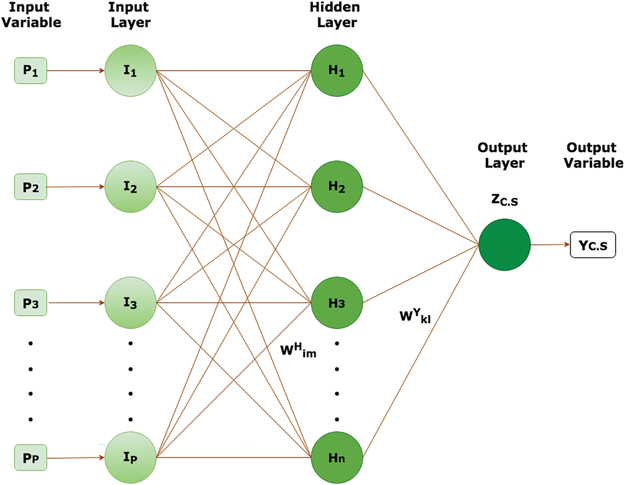
Figure 1: ANN architecture with single hidden layer

Choosing the number of hidden layers and neurons in each hidden layer is a core element that has a high influence on the system soundness. The training algorithm is also the crucial component of the FFNN [45]. MSE is used as the objective function in the majority of ANN training algorithms. The difference between the expected (model results) and observed (lab testing) responses is known as the MSE.

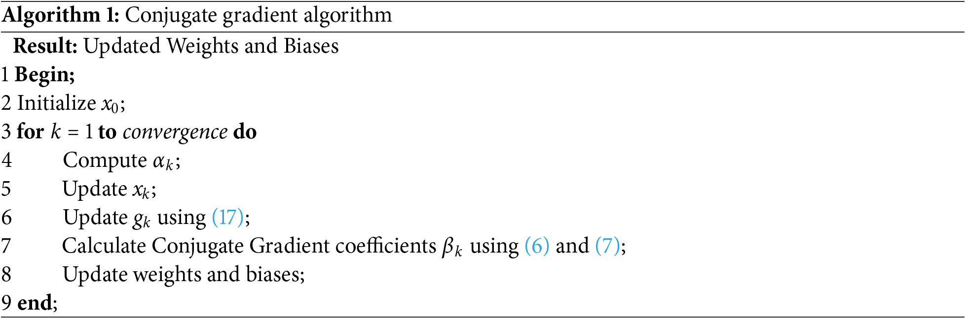
As far as the training of ANN with feedforward architecture is concerned, literature proposes various training algorithms. The most popularly employed training algorithms are Bayesian Regularization (BR), Conjugate Gradient with Powell/Beale Restarts (CGB), Fletcher-Powell Conjugate Gradient (FP-CG), Polak-Ribiére Conjugate Gradient (PR-CG) and Levenberg-Marquardt (LM) which are also considered in the present study.

1.2 Conjugate Gradient (CG)

Conjugate Gradient (CG) is a frequently used iterative process for determining the values of weights and bias (parameters of ANN) and is reputable for its prompt convergence rate. Some of its editions include CGB, FP-CG, PR-CG, and scaled conjugate gradient (SCG), etc. Fundamentally training starts with initialization process where random values x0 are assigned to parameters linked to individual variables in input layer along with initialization of search direction as

d0=∇f(w0)(2)

In each iteration, values of parameters are updated by defining the step size in terms of αk and gradient to update the search direction using following equations

wk+1=wk+αkdk(3)

gk+1=∇f(wk+1)(4)

Basically conjugate gradient method is focused to calculate coefficient of conjugate gradient βk which is the updated search direction in each iteration as

dk+1=gk+1+βkdk(5)

1.2.1 Conjugate Gradient with Powell/Beale Restarts

In conjugate gradient with Powell/Beale Restarts iterations are resumed periodically to accelerate and to resolve probable convergence problems. The intrinsic idea is to restart the iterative process when the optimization process starts to lag. Usually a restart condition is defined based on the number of iterations, convergence threshold or step-size threshold. Algorithm 1 explains the basic steps of the conjugate gradient algorithm.

1.2.2 Fletcher-Powell Conjugate Gradient (FP-CG)

The Fletcher-Powell version of the conjugate gradient method uses a different formula for calculation of the conjugate gradient coefficients βk.

βk=∇fk+1T.∇fk+1∇fkT.∇fk(6)

1.2.3 Polak-Ribiére Conjugate Gradient (PR-CG)

This variant of conjugate gradient employs different equation for conjugacy coefficient.

βk=(∇fk+1−∇fk)T.∇fk+1∇fkT.∇fk(7)

1.3 Bayesian Regularization

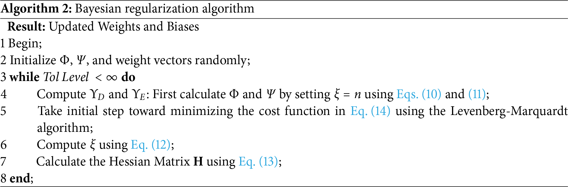
The regularization parameters tuning with Bayesian requires calculation of minimum point Pmin from Hessian matrix of a given function F(w) [46]. The aim of the Hessian matrix-based update in Bayesian regularization is to include the curvature of the loss function in the weight updates. The update rule in consecutive iterations can be expressed as follows:

∇Wk=−[∇T(Wk)∇(Wk)+ζkI]−1∇T(Wk)V(Wk)(8)

where ∇(W) is a Jacobian Matrix and ζ is a step controlling parameter and Vw is the sum of squares function:

F(w)=∑i=1NV12(W)=(VT)(W)V(W)(9)

The regularization parameters Φ and Ψ with relations are defined as;

Φmin=ξ2ΥDWmin(10)

Ψmin=N−ξ2ΥDWmin(11)

where ξ is number of effective parameters used to reduce error function defined as;

ξ=n−2Φmintr(Hmin)−1(12)

where n is the total number of parameters in network and H is the Hessian matrix which can be calculated as;

H=2Ψ∇T∇+2ΦIn(13)

With updated values of Φ and Ψ, the objective function can be defined as;

F(W)=ΨΥD+ΦΥE(14)

Algorithm 2 summarizes the fundamental steps of the Bayesian regularization algorithm.

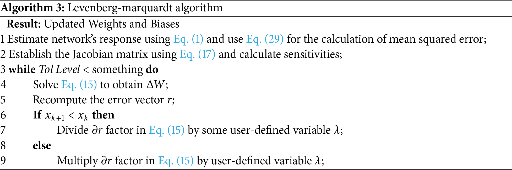
1.4 Levenberg-Marquardt Framework

The Levenberg-Marquardt (LM) algorithm is an optimization technique most frequently used to solve nonlinear least squares problems that aspires to reduce the sum of the squares of the variations between observed and predicted values and usually works in conjunction with the steepest descent method [27]. This algorithm starts with assigning of initial values of hyper parameters (weights and bias) and a small positive value for the damping component λ. This algorithm reportedly offers faster convergence, improved stability and owing to adaptive damping, it is reliably more resilient when data is noisy or contains outliers. Let us assess the output return of FFNN, calculated using (1), where initial output response is given as YC.S and the error of the network is calculated using (29). Originated from the steepest descent method, the rule to update LM algorithm is defined as;

ΔW=(JwrTJwr+δrI)−1JwrTr(15)

and updated parameters in each iteration can be given as;

Δxk=−[JwrTxkJwrxk+δrI]−1JwrT(xk)v(xk)(16)

where Jwr has dimensions of (P×Q×R) and the matrix of dimensions (P×Q×1) is defined as error matrix. So the Jacobian matrix is established using the following association:

Jwr=[∂r11∂w1∂r11∂w2…∂r11∂wR∂r11∂b1∂r12∂w1∂r12∂w2…∂r12∂wR∂r12∂b1⋮⋮⋮⋮⋮∂r1Q∂w1∂r1Q∂w2…∂r1Q∂wR∂r1Q∂b1⋮⋮⋮⋮⋮∂rP2∂w1∂rP2∂w2…∂rP2∂wR∂rP2∂b1∂rP2∂w1∂rP2∂w2…∂rP2∂wR∂rP2∂b1⋮⋮⋮⋮⋮∂rPQ∂w1∂rPQ∂w2…∂rPQ∂wR∂rPQ∂b1](17)

Here, R denotes the total number of weights and elements in the error vector, while r is computed using Eq. (17). P represents the number of training patterns, each associated with Q output values. Traditionally, the Jacobian matrix Jwr is first computed, and then calculations for updating weights and biases are carried out using values that have been stored. This approach operates smoothly and effectively with lesser patterns, but memory constraints arise while calculating the Jacobin matrix for big patterns. Algorithm 3 enlists the fundamental steps of the standard LM algorithm that generates the Jacobian matrix and later calculates the sensitivities. We can also conclude that the LM algorithm’s performance decreases with large training sets.

1.5 XGBoost Model

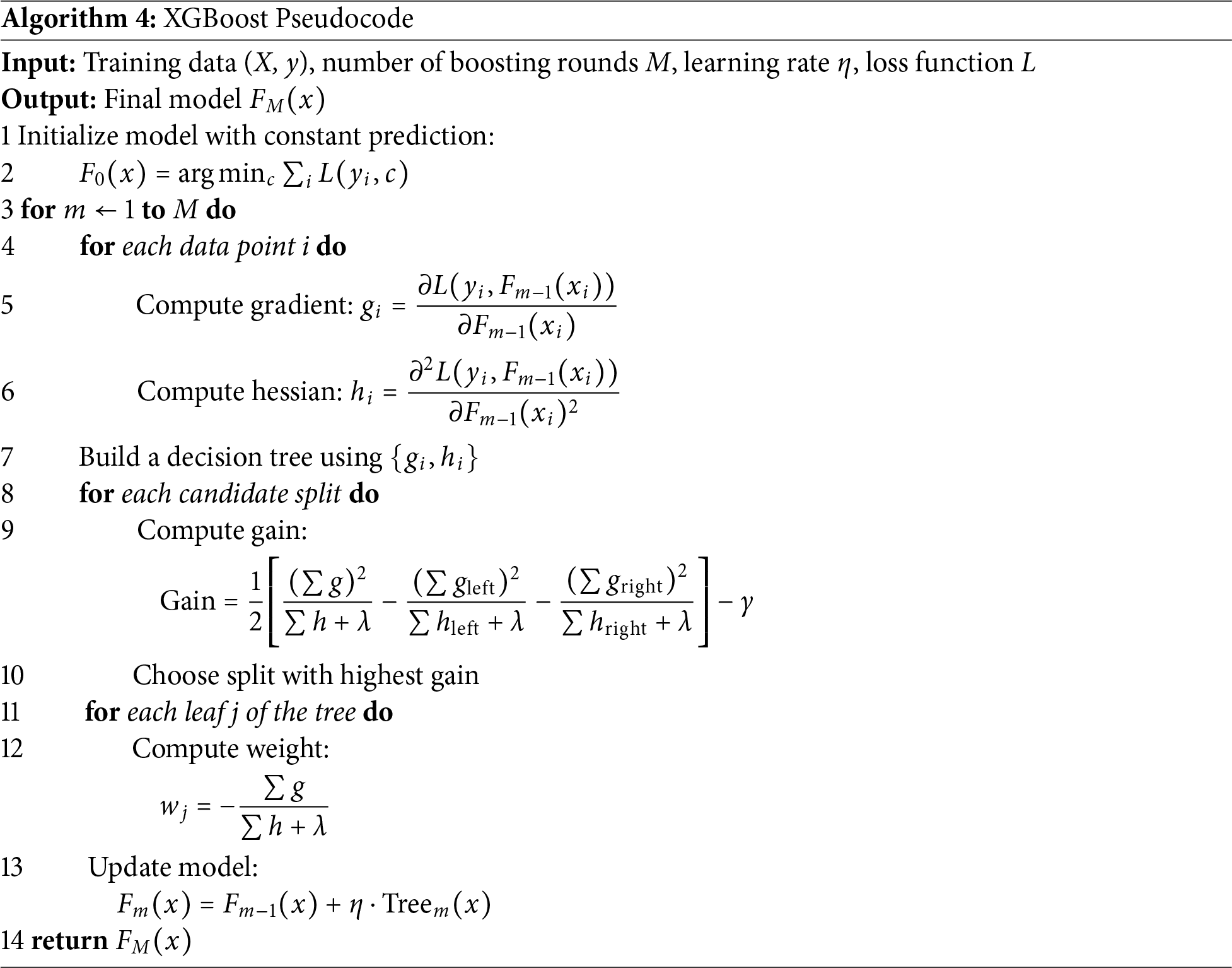
Boosting is an ensemble learning strategy which generates a powerful regression model by combining several weak learners with the idea that every new model is trained to reduce the errors of the ones that were trained before. The final ensemble model achieves excellent accuracy and robustness by upgrading one step at a time. It greatly enhances traditional gradient-boosting models by integrating second-order gradient information, hence refining the optimization process [47]. The training of the dataset (X,y) starts with defining the number of boosting rounds M, the learning rate η, and a specified loss function L. The model is first initialized with a constant prediction that minimizes the loss:

F0(x)=arg⁡minc∑i=1nL(yi,c)(18)

As the error is measured in terms of mean squared error (MSE):

F0(x)=arg⁡minc∑i=1n(yi−c)2ddc∑i=1n(yi−c)2=−2∑i=1nyi+2nc=0c=1n∑i=1nyi∴F0(x)=y¯(19)

At each boosting round, a new decision tree is constructed to correct the errors of the current model. For each data point i, compute the gradient as first derivative and hessian as second derivative of the loss function with respect to the current prediction:

gi=∂L(yi,Fm−1(xi))∂Fm−1(xi)(20)

hi=∂2L(yi,Fm−1(xi))∂Fm−1(xi)2(21)

A classification and regression tree (CART) decision tree is built using the computed gradients and hessians from (20) and (21).

For each candidate split, the gain is calculated as:

Gain=12[(∑g)2∑h+λ−(∑gleft)2∑hleft+λ−(∑gright)2∑hright+λ]−γ(22)

where λ is the regularization term on leaf weights, and γ is the penalty for additional leaves. The split with the highest gain is chosen. For each terminal leaf j, the optimal weight is computed as:

wj=−∑g∑h+λ(23)

This determines the prediction adjustment that the leaf contributes. The new tree is added to the model with learning rate η:

Fm(x)=Fm−1(x)+η⋅Treem(x)(24)

After M iterations, the final boosted model is obtained:

FM(x)(25)

This ensemble of decision trees provides strong predictive power, balancing accuracy and generalization through regularization and learning rate scaling. Fig. 2 describes the detailed workflow of the development of XGBoost regression model, whereas the fundamental steps are given in Algorithm 4.

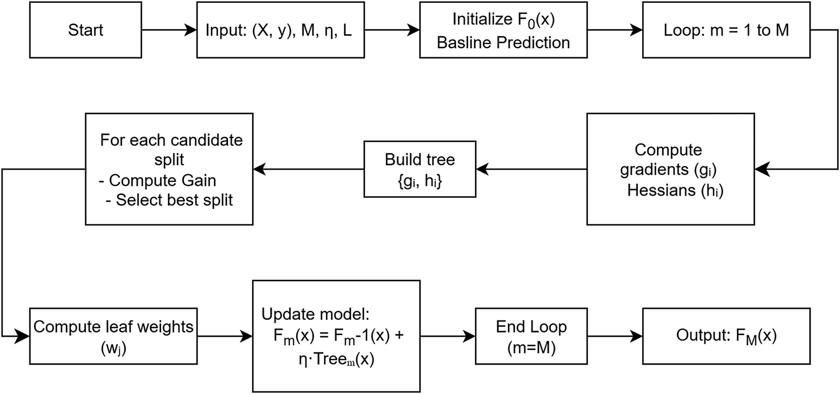
Figure 2: XGBoost Workflow (Newly added figure)

1.6 Random Forest Model

Random forest (RF) is an ensemble techniques developed for classification and regression by Leo Breiman at the University of California, Berkeley [48]. The training of the dataset (X,y) commences with the specification of the number of trees M, the number of features to sample m at each split, and the number of bootstrap samples per tree n. Draw a bootstrap sample of size n from the training set (X,y) for every tree t=1,…,M. As every tree does not see the same data, this adds randomization and lowers variance. To grow each decision tree, the bootstrap sample is used. Choose a random subset of m features from the entire feature set at each split node. As a result, there is less association between trees and tree diversity is guaranteed. For regression, the split is chosen to minimize the MSE. The impurity at a node with dataset S is measured as:

MSE(S)=1|S|∑i∈S(yi−y¯S)2(26)

where y¯S is the mean of the target values in S. The best split is the one that maximizes the reduction in impurity:

Δ=MSE(S)−(|Sleft||S|MSE(Sleft)+|Sright||S|MSE(Sright))(27)

In its terminal leaf, each tree outputs the mean value of the training samples in order to make a prediction. The average of each tree yields the RF prediction:

1M∑t=1MTreet(x)(28)

After M trees, the final trained random forest regression model FM(x) is obtained.

Algorithm 5 explains the fundamental steps of the random forest algorithm—starting from the initialization to the final output of all tree predictions.

2  Methodology

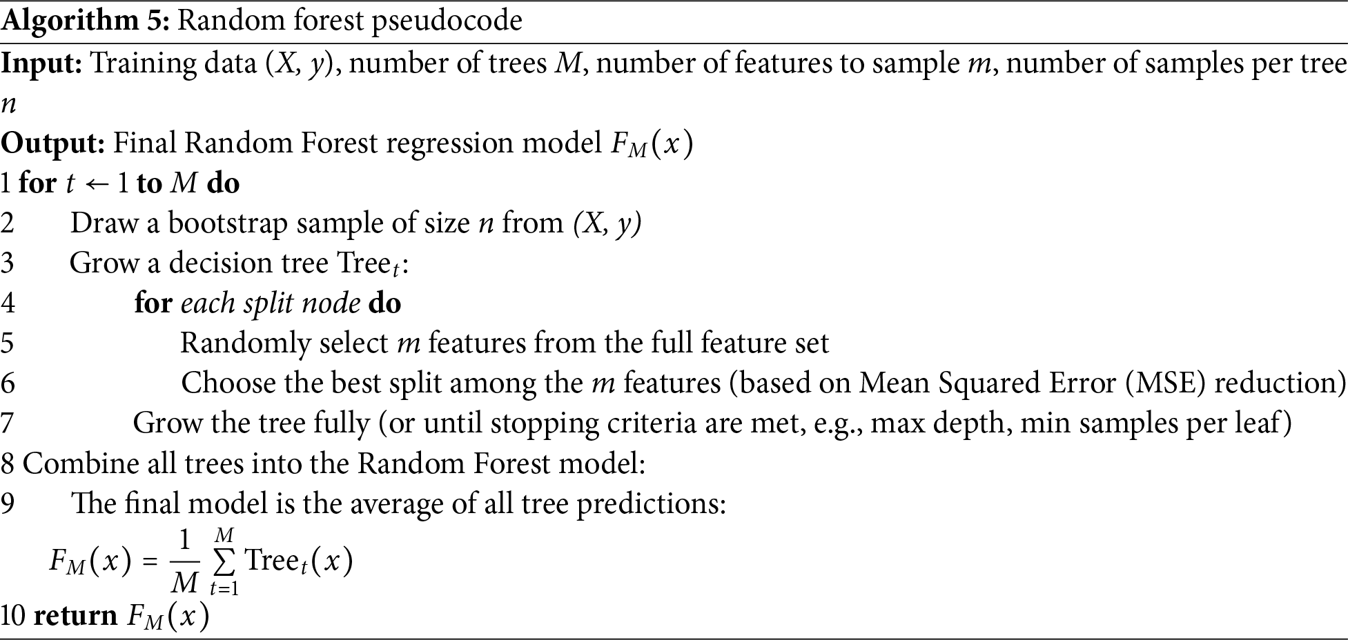
Fig. 3 summarizes the research technique used to develop a predictive model for determining CS of concrete having RAs.

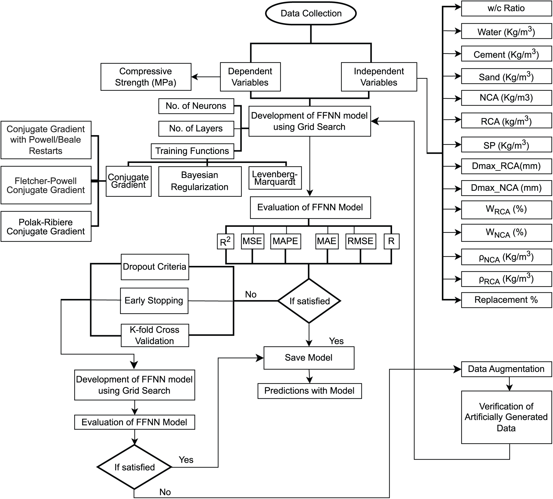
Figure 3: Methodology for concrete compressive strength prediction using FFNN

2.1 Dataset Description

Concrete with RAs has distinct fresh and hardened characteristics from concrete manufactured using NAs. When compared with NAs, RAs absorb more water and have lower density [9]. Other possible reasons for reduced strength in concrete are the presence of residual mortar on the aggregate surface, poor gradation due to improper crushing, age, and strength of the demolished structure, etc. Owing to these factors, with an increase in the RA content, the mechanical characteristics decrease [49]. Thus, the fundamental elements of regular concrete, which are cement, water, sand, superplasticizer, and coarse aggregates (in terms of their bulk density, water absorption capacities, and size), along with other parameters describing the properties of RAs, i.e., size, density, and water absorption of RAs, are considered input factors influencing the hardened concrete CS. Present research considers a data set that includes 501 data points collected from the published literature. The statistics of the input and output variables (mean, median, mode, standard deviation, minimum, and maximum) are listed in Table 1. The distribution of the data used is shown in Fig. 4. The replacement ratio of RAs with natural coarse aggregates (NCA) mainly takes values around 0 %, 25%, 50%, and 100%. The 0% indicates samples having 100% natural aggregates as reference samples. The bulk density of recycled coarse aggregate and the bulk density of natural coarse aggregates ranges from 2200 to 2800 kg/m3; the water absorption capacity of recycled coarse aggregates is mainly distributed in 2%–10% while the water absorption of natural is distributed in 0.2%–3%.

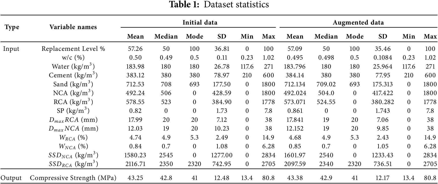
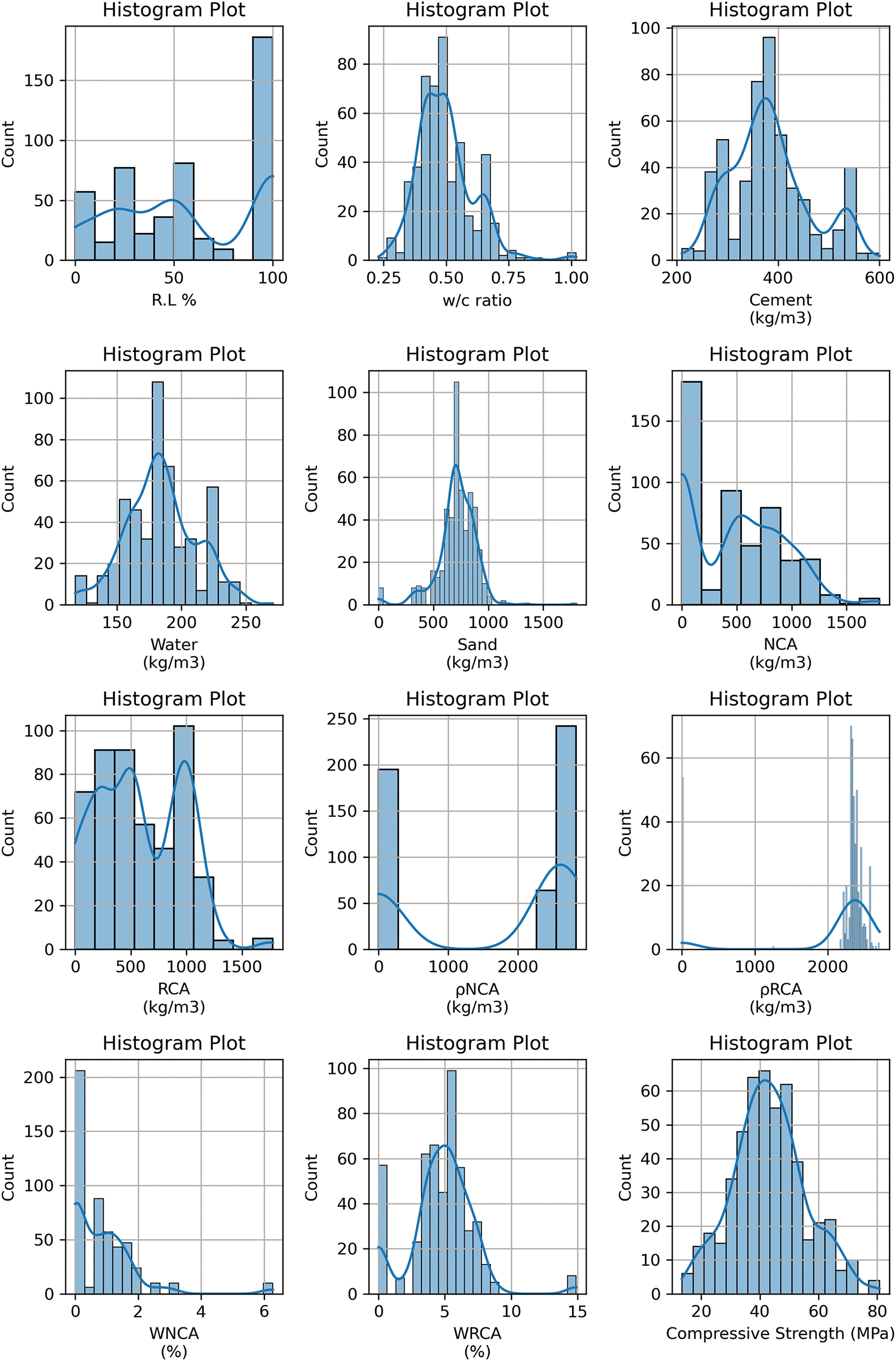
Figure 4: Histograms of the variables in the dataset

Fig. 5 demonstrates the multiple correlation matrix of the input features and output used in the present study. The Pearson correlation coefficient between variables is displayed visually in each cell of the heatmap, which offers a depiction of the correlation matrix [50]. The color tones represent the strength of the relationships. Most of the correlations between variables are pretty weak (less than 0.5), but some have strong correlations, like the highest correlation found between R.L% and content of RAs (R = 0.94). Similarly, water absorption capacity, density, and content of RAs are highly correlated, and the same is visible for water absorption capacity, density, and content of NAs. Since ANNs can handle correlated features without compromising model stability, and because their inclusion enables the network to learn complex, nonlinear interactions that could be lost if variables were removed, multicollinearity among some input parameters was kept in place despite their existence.

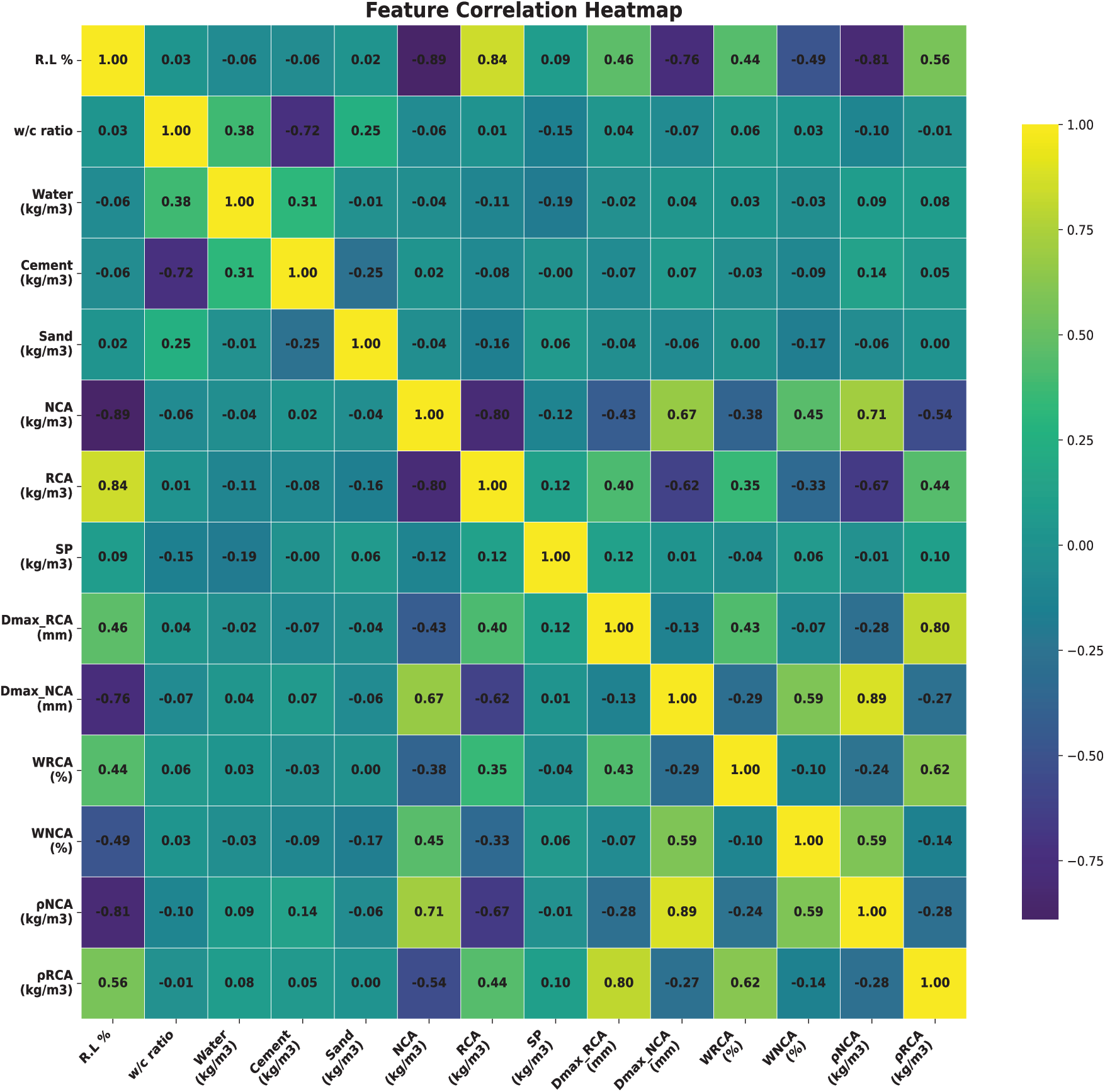
Figure 5: Correlation matrix for variables

2.2 Data Preprocessing

While training ANNs, normalization is crucial since it assure that all features contribute equitably to the learning process and avoids some attributes from dominating others due to disparities in their magnitude.

2.3 Model Development

The evolution of the prediction model intricate numerous intervals, each targeted on improving the performance of model.

2.3.1 Grid Search for Hyperparameter Tuning

The formulation of ML models entails identifying the ideal values of hyperparameters for model [14]. To achieve best combination of hyperparameters such as the number of layers and their respective neurons, and the training function, a grid search approach was employed. Grid search is a comprehensive, autonomous search technique that determines the optimal performance by analyzing each potential hyperparameter combination in the search space [51].

2.3.2 Dropout Regularization

To prevent overfitting and increase generalization, dropout regularization with 20% probability was utilized. Dropout regularization involves dropping a fixed percentage of neurons to prevent the neural network from memorizing the learning patterns and to make it more robust, allowing it to generalize better to new, unseen data.

2.3.3 Early Stopping

Early stopping is an approach for reducing excessive learning that involves identifying the time at which overfitting begins during training of neural network model via cross-validation [52]. To reduce overfitting and improve training efficiency, early stopping criterion was used. Training was ended if the performance of model did not improve for 10 consecutive epochs.

2.3.4 Data Augmentation

Due to the limited dataset size and the desire to improve model generalization, data augmentation is usually performed by various researchers. Reference [18] used data augmentation technique to forecast CS of calcined clay cements using linear regression. Reference [53] used data enhancement technique in Convolutional Neural Networks (CNNs) training to proficiently develop a synthetic dataset of concrete cracks in concrete. Using this technique effectively increased the dataset size preserving the intrinsic associations between features and the target variable.

By using linear interpolation between preexisting data points, a data augmentation technique was used to expand the dataset size while maintaining its statistical characteristics. This produced new samples that stayed within the observed range of variables. Clipping with predetermined conditions was used to avoid generation of absurd data points. The replacement level (R.L%), was tightly limited to a range of 0%–100%. Additionally, all characteristics of RCAs were set to zero when NCAs were utilized without any replacement. On the other hand, the NCA attributes were set to zero when RCAs were utilized exclusively. These boundary specifications preserved the overall distributions and correlations of the original dataset while ensuring that the augmented data remained logically meaningful and statistically representative.

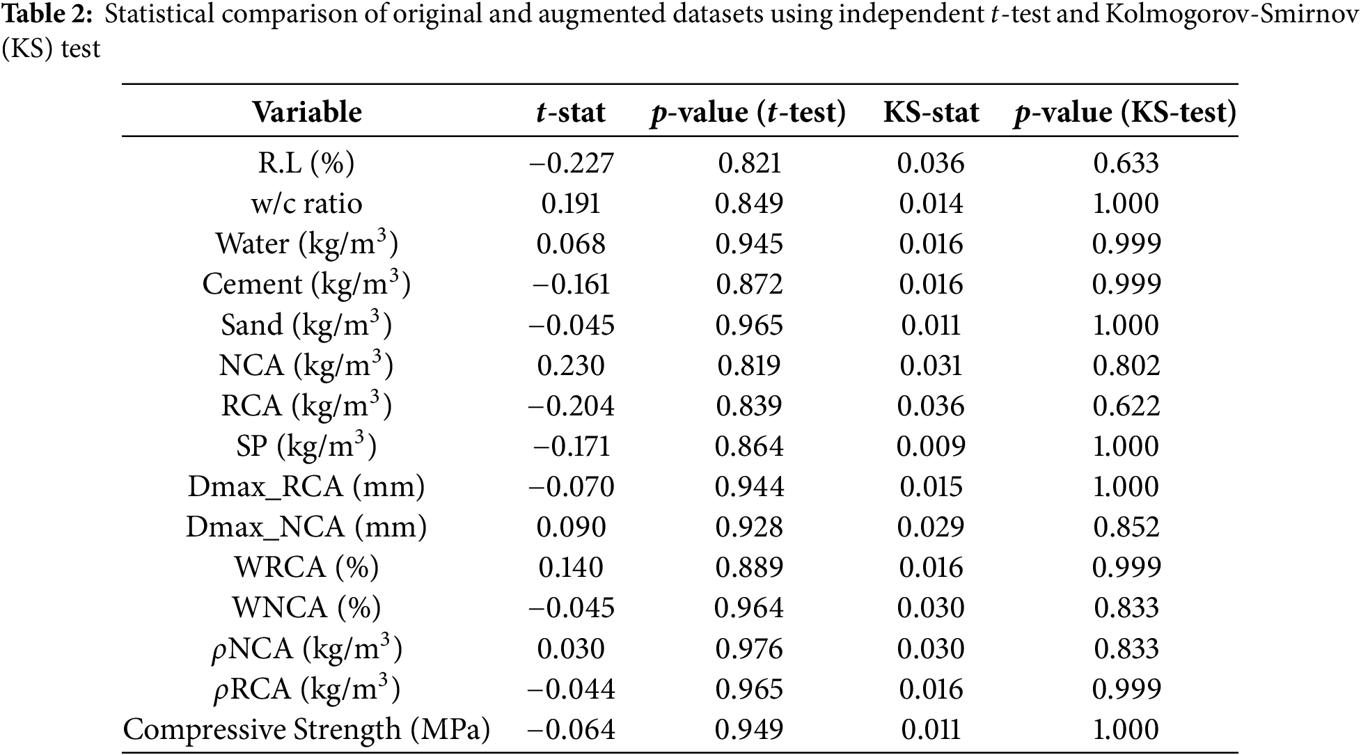
Independent two-sample t-tests and Kolmogorov-Smirnov (KS) tests were performed on each numerical feature to ensure that the augmented dataset preserved the statistical consistency with the original dataset. The t-tests assessed differences in feature means, while the KS tests evaluated the similarity of their overall distributions.

Both the t-tests and KS-tests as shown in Table 2 yielded non-significant results (p > 0.05 for all variables), confirming that the augmented dataset is statistically indistinguishable from the original.

2.4 Model Evaluation

Once the prediction model is developed, its performance must be assessed. The model evaluation indices used in this paper are MSE, RMSE, R, R2, MAPE and MAE. MSE calculates the variation of anticipated and observed responses while R2 evaluates the feasibility, viability, and linearity of the model. MAPE measures the average absolute difference in percentage between forecasted values and actual values whereas MAE gauges the average absolute difference between anticipated and actual values.

MSEC.S=12(∑C.S=1M(yC.S−dC.S))=12(∑C.S=1M(rC.S)(29)

In (29), MSE is calculated where yC.S stands for the predicted values, dC.S stands for the actual values, and rC.S stands for the residuals.

RMSEC.S=1M∑i=1M(yC.S−dC.S)2(30)

R=∑i=1M(Xi−X¯)(Yi−Y¯)∑i=1M(Xi−X¯)2∑i=1M(Yi−Y¯)2(31)

In (31), Xi and Yi represent paired observations, where Xi is the explanatory variable and Yi is the response variable. The mean of the response variable Y is denoted by Y¯ and average of explanatory variable X is X¯.

R2=1−∑i(dC.S−y^C.S)2∑i(dC.S−Yi¯)2(32)

MAE=1M∑i=1M|yC.S−dC.S|(33)

MAPE=1M∑i=1M|yC.S−dC.SdC.S|×100%(34)

2.5 Sensitivity Analysis

The sensitivity analysis of a AI based regression model is a strategy which is adopted to discover if the predicted value is altered by variations in the assumptions of the independents [54].

2.5.1 Perturbation Sensitivity Analysis

Reference [55] scrutinize different perturbation based sensitivity analysis approaches on modern transformer model to gauge their performances. This method initially uses a generated model to make predictions, then introduce random noise to perturb it while preserving the integrity of all other aspects and finally inspects the predictions using the perturbed input features. Ultimately the difference is calculated using

Sensitivityj=1n∑i=1n|targetOutputi−targetOutputperturbedi|(35)

In (35), Sensitivityj is the sensitivity of the output of the model to the perturbation of the jth input feature, n is the number of samples in the dataset, while targetOutputi is the original predicted output for the ith sample using the original input features and targetOutputperturbed is the predicted output for the ith sample using the perturbed input feature j.

2.5.2 Weight-Partitioning Sensitivity Analysis

In context of ANNs, the weight matrix (W) is generated from the developed model and has dimensions of i×j where i is the number of neurons in the first layer and j is the number of input features. Larger absolute weights associated with neurons indicates greater influence on output. From the absolute weights, total contribution for each input feature is calculated using (36) where for each neuron m and input feature n;

Cn=∑x=1m|wmn|(36)

2.6 Partial Dependence Plot

Partial dependence plots (PDPs) display the slight impact of one or a small number of input features on an anticipated result of ML model. The key concept is that, while maintaining other characteristics constant, PDPs offer a transparent, graphical representation of how small modifications to the inputs impact the prediction [56]. This helps illustrate if a feature has a linear, monotonic, or complicated relationship with the target. However, PDPs presume feature independence, which can result in false interpretations if features are correlated [57]. Mathematically, for a feature xj:

f^pd(xj)=1n∑i=1nf^(xj,xij)(37)

Here, xij represents all features except xj, and f^ is the predictive model.

2.7 Accumulated Local Effects

By calculating the local impact of a feature on the prediction of ML model, accumulated local effects (ALE) plots are intended to help interpret intricate machine learning models [58]. ALE avoids extrapolating into irrational areas of the feature space and takes feature correlations into consideration, in contrast to PDPs. Because of this, ALE works particularly well with correlated and high-dimensional datasets. The local effect of feature xj at a point x is the partial derivative of the model with respect to that feature:

ϕj(x)=∂f^(x)∂xj(38)

This measures how much the prediction changes locally if we change only xj. Since derivatives are noisy and localized, ALE integrates them across the xj range. Suppose the domain of xj is split into intervals:

z0<z1<⋯<zK

with K bins. For a bin k=1,…,K, the ALE effect increment is:

Δj(k)=E[∫zk−1zk∂f^(xj,xj)∂xjdxj | xj∈[zk−1,zk]](39)

Here, xj are all features except xj. The conditional expectation ensures we only integrate where data actually exists. The ALE function for feature j at point zk is the accumulated sum of increments up to that bin:

f^ALEj(zk)=∑l=1kΔj(l)(40)

To make ALE functions comparable and remove arbitrary offsets, they are centered:

f~ALEj(zk)=f^ALEj(zk)−1K∑k=1Kf^ALEj(zk)(41)

This gives a function showing how predictions accumulate as xj increases. This ensures:

E[f~ALEj(xj)]=0(42)

f~ALEj(zk)=∑l=1kE[∫zl−1zl∂f^(xj,x∖j)∂xjdxj | xj∈[zl−1,zl]]−1K∑k=1Kf^ALEj(zk)(43)

3  Results

The first and the most critical step in developing an ANN model that is best suited to the given challenge is to select a neural network design which may include number of layers, number of neurons, architecture, training function, activation function, learning rate, number of iterations/epochs, etc. In the present study, five different optimizers/training functions (BR, LM, CGB, FP-CG, and PR-CG) have been used for model training and are compared based on MAE, MAPE, R, R2, MSE, and RMSE to assess the model performance. A total of 125 FFNN models have been developed based on different numbers of hidden layers, hidden layer neurons, and training functions with grid search. When grid search was conducted initially, best training function came out to be FP-CG with two hidden layers having 30 and 10 neurons in first and second layer consecutively as shown in Table 3. The accuracy of the model developed in terms of coefficient of determination R2 = 0.7627 which is not acceptable by literature.

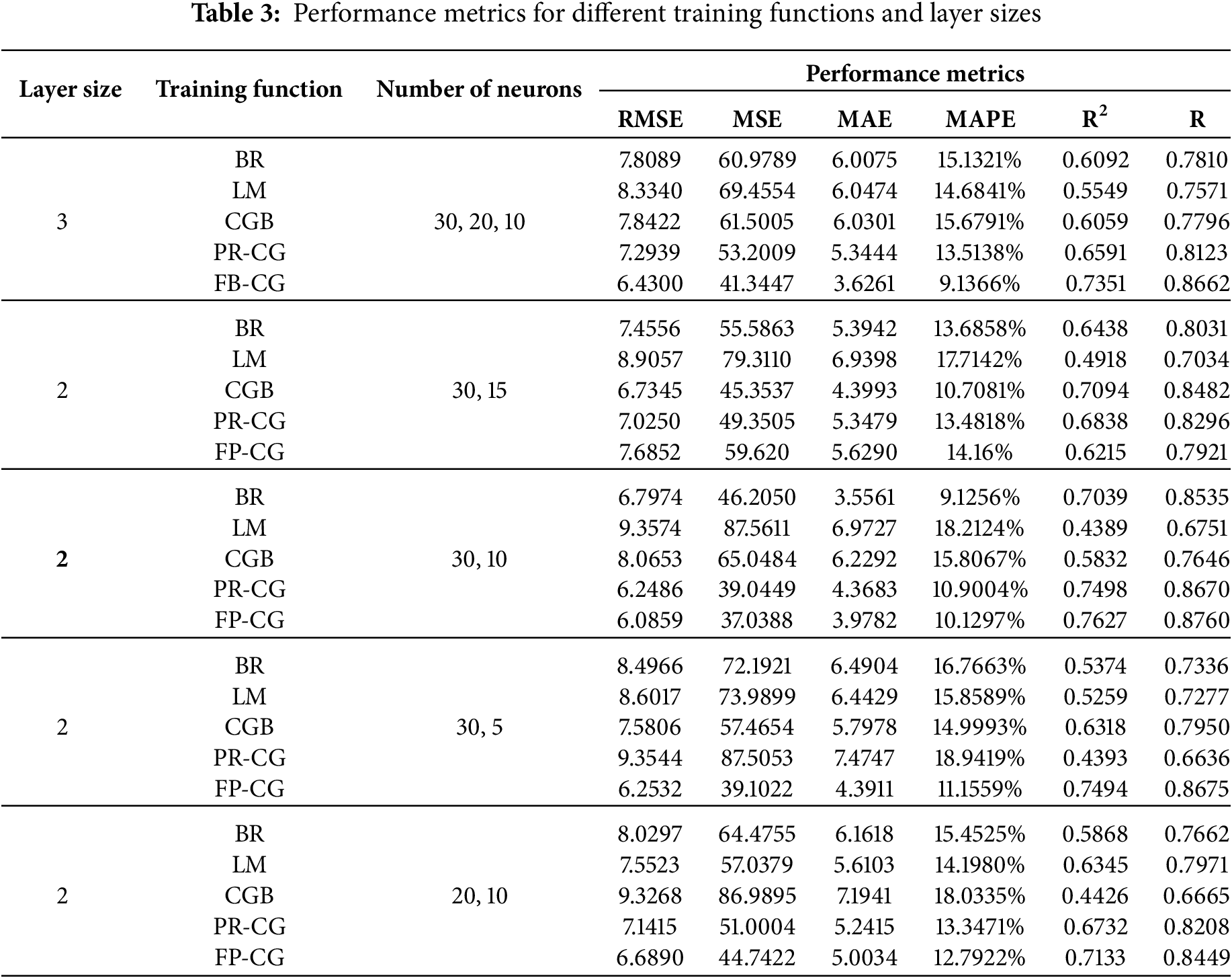
Table 4 shows the results of the RF and XGBoost model trained using raw data collected from literature.

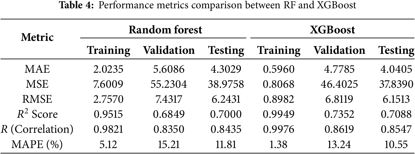
Fig. 6 shows the performance curve of ANN with FP-CG. The plot shows the MSE for training, validation, and testing datasets over 1000 epochs. The performance plot shows best performance at 411 epoch with least MSE, but as training is called for 1000 epochs, training continues resulting in decrease in accuracy. To avoid overfitting early stopping was applied, which did not show any significant improvement. With early stopping LM optimizer, with two hidden layers having 30 and 15 neurons respectively performed well. Fig. 7 reveals the performance of FFNN trained on literature-based data, comparatively lower predictive accuracy, as evidenced by greater dispersion from the ideal prediction line.

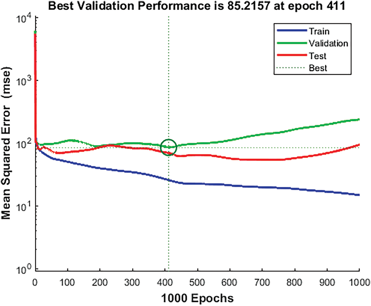
Figure 6: Performance of neural network training with FP-CG

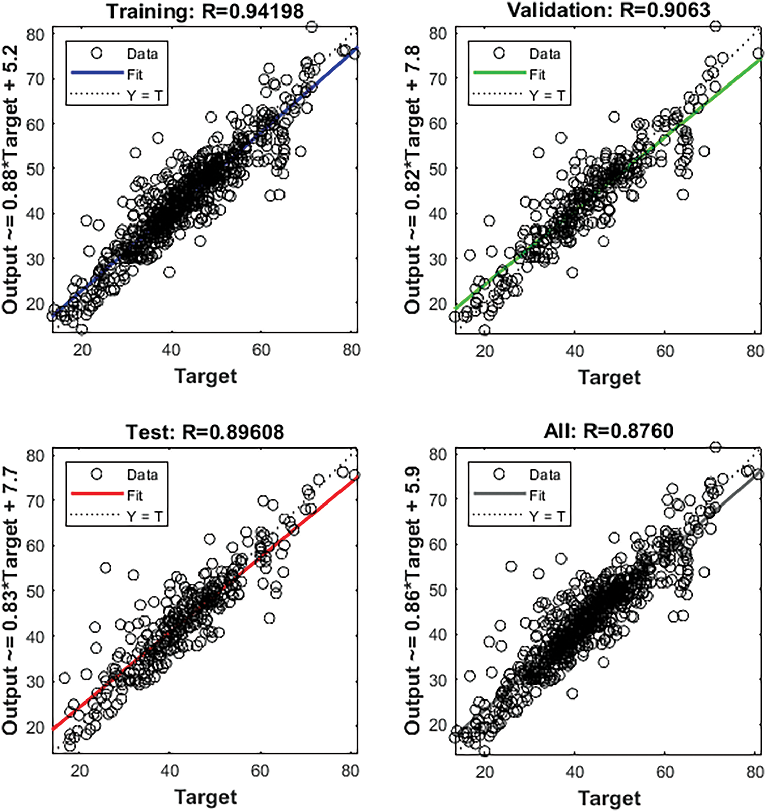
Figure 7: Neural net training with FP-CG

It can be seen from Table 5 that the optimal FFNN structure was 30-20-10, with a R2 of 0.9669; the MAE was 0.873, with the hyperbolic tangent sigmoid activation function for hidden layers and default activation function for the neurons in the output layer is the purelin (linear transfer function). It also demonstrates that performance remains consistent across the three datasets, clearly indicating that the FFNN utilizing the LM optimizer for training surpasses all other models.

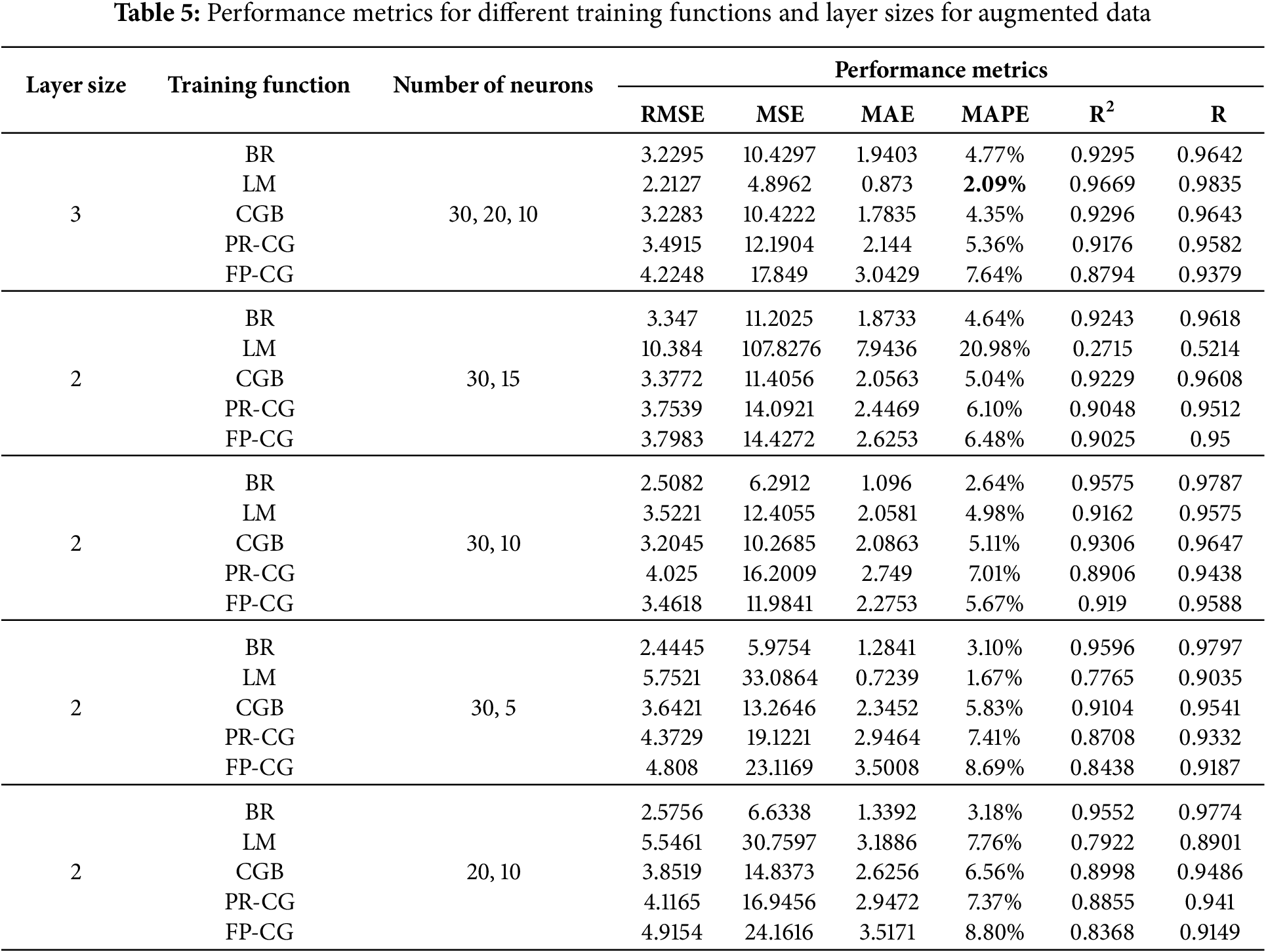
Table 6 presents the accuracy metrics results for the RF and XGBoost models. Both models exhibited strong performance on the training dataset; however, their effectiveness diminished when evaluated on the validation and testing datasets, indicating evident signs of overfitting. Fig. 8 illustrates that the Levenberg-Marquardt-trained neural network achieved its best validation performance (MSE = 27.0455) at the final epoch, indicating stable and effective learning from augmented data.

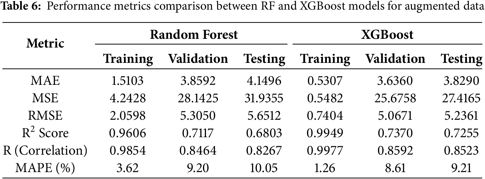
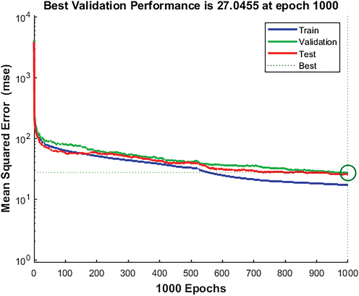
Figure 8: Performance of neural network training for augmented data with LM

Fig. 9 demonstrates enhanced alignment and reduced prediction error when the model is trained on augmented data, thereby confirming the efficacy of data augmentation in improving model performance. The comparative scatter plots in Fig. 10 reveal that all three models—FFNN, RF, and XGBoost—exhibit strong predictive alignment between actual and predicted values across training, validation, and testing subsets. Notably, the FFNN model demonstrates superior consistency and accuracy, as evidenced by its tighter clustering along the ideal prediction line.

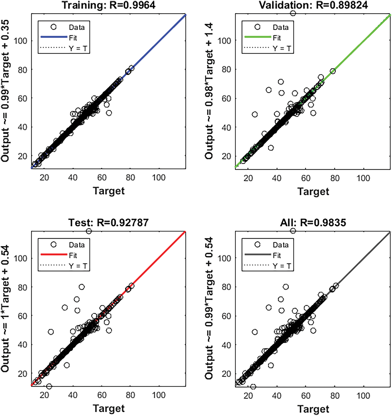
Figure 9: Neural net training for augmented data with LM

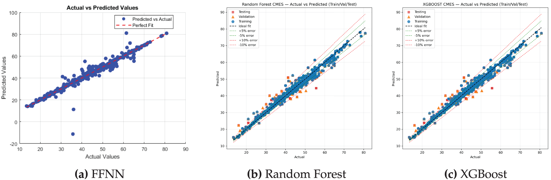
Figure 10: Comparison of Actual vs. Predicted values for different models

Fig. 11 expresses that the model trained on collected and augmented data generates predictions of CS that closely approximate the true values. Fig. 12 is a 3D bar graph, highlights the importance of synergizing the right neural network architecture with an appropriate training function. It depicts six assessment parameters (RMSE, MSE, MAE, MAPE, R2, and R) for multiple layers and training function layouts in a neural network for augmented data. The x-axis illustrates distinct layer configurations, the y-axis shows the values of different assessment parameters, while the z-axis narrates different training functions used in grid search for hyperparameter tuning. It is apparent that the LM training function, paired with the 30-20-10 layer configuration, generates the most accurate results. This coalition depicts the lowest MSE, representing minimal error in forecasting, and the highest R2 value, expressing a powerful alignment between the predicted and actual data.

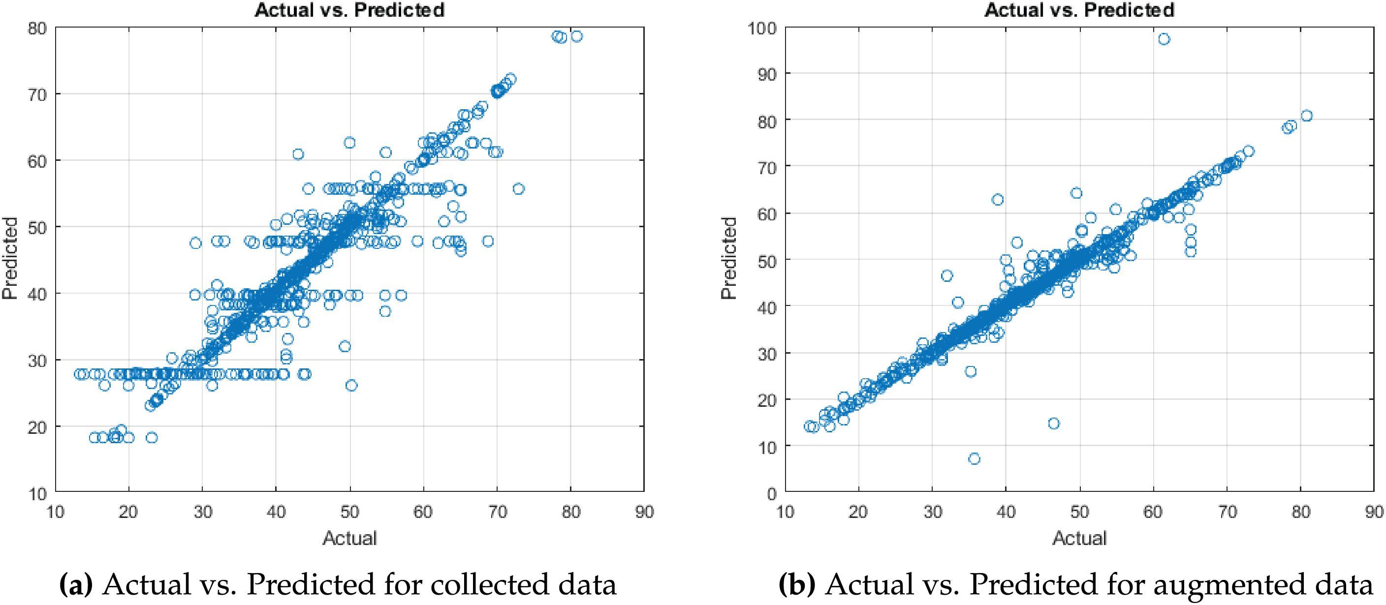
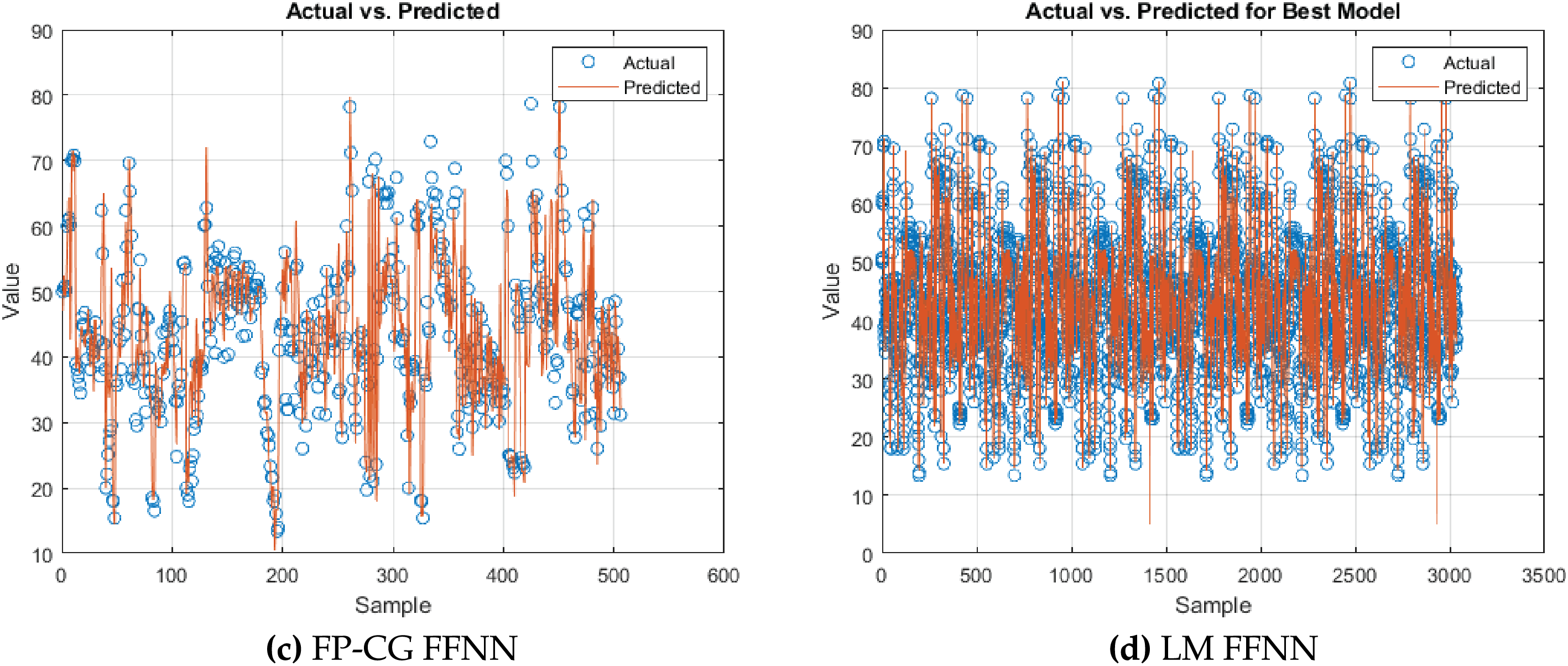
Figure 11: Comparison of model performance for collected and augmented data

Figure 12: 3D bar chart for comparison of performance of different optimizers

3.1 Sensitivity Analysis

Fig. 13 highlights the influence of various input variables on the predicted CS of concrete containing RAs. The results of the perturbation analysis reveal that cement has the most significant effect, whereas the weight partitioning sensitivity analysis reveals that water has the utmost influence on strength. Furthermore, based on weight-partitioning sensitivity analysis, cement is the second most influential factor. This result is consistent with the widely approved fact that cement being main component of concrete has a significant impact on its strength. CS of concrete is eventually determined by the chemical reactions and hydration processes that are directly influenced by the quantity, quality, and composition of the cement. The presence of water is vital in concrete, as it initiates and sustains the hydration process, allowing cement to react with other components and form a strong bond [55]. But with too much amount of water, pores get saturated leaving gaps, which weakens the material. Other parameters that can influence, presence of admixtures, the temperature at the time of hydration, and aggregate and cement paste interface [59]. From 13, other than water and cement, superplasticizer and water absorption are the other important factors.

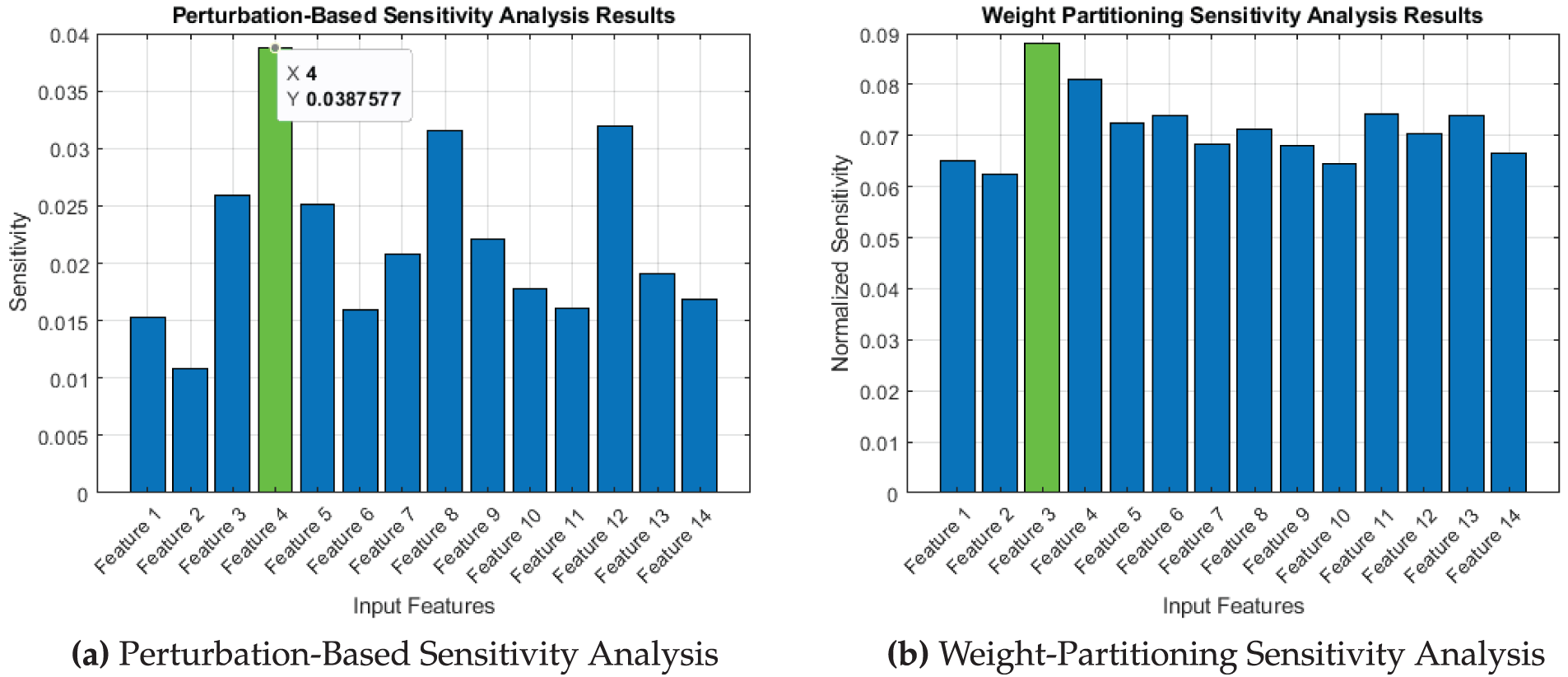
Figure 13: Sensitivity analysis of FFNN trained model using LM optimizer

Figs. 14 and 15 show consistent results that water to cement ratio is the most influential factor for both the RF and XGBoost models.

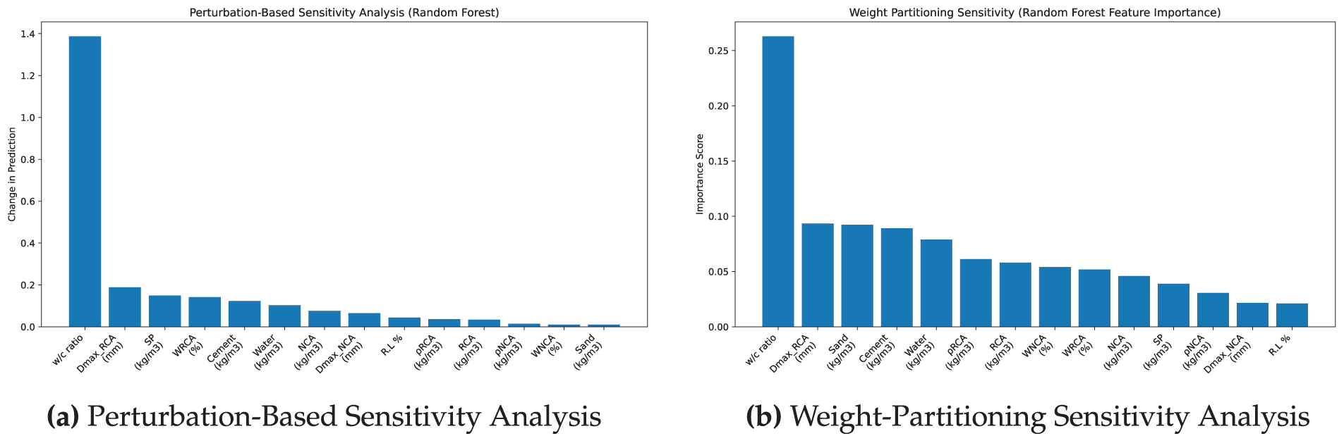
Figure 14: Sensitivity analysis of RF model

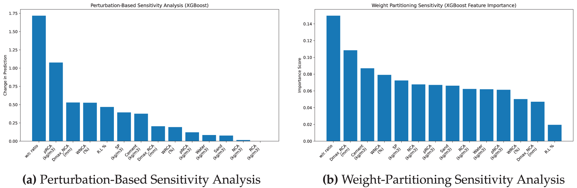
Figure 15: Sensitivity analysis of XGBoost model

3.2 Partial Dependence Plots

Fig. 16 shows the PDPs analyses of all the three models which clearly indicate that the presence of cement and superplasticizer contributes positively to the predicted strength. Conversely, increased water-to-cement ratios and the properties of RAs lead to a decrease in strength. While XGBoost is adept at identifying more pronounced nonlinear relationships, both models demonstrate trends that are consistent with domain knowledge, even though PDPs may have limitations in scenarios involving correlated features.

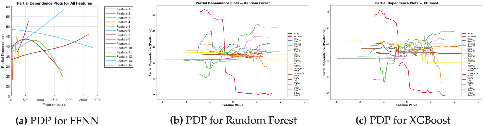
Figure 16: Comparison of PDPs for different models

3.3 Accumulated Local Effects

Fig. 17 illustrates the aggregated localized impacts of the input features on the outputs of the three models employed in this investigation. The RF and XGBoost models exhibit identical behavior. The enhancement of compressive strength is primarily influenced by the presence of cement, sand and SP. Conversely, higher water-to-cement (w/c) ratios result in reduction in matrix density, while excessive RCA content is linked to lower quality, increased porosity, and weaker interfacial zones. In contrast, NCA content has a positive impact, and other factors such as maximum aggregate size (Dmax) and absorption capacities exhibit relatively minor or negligible effects within the examined range. While the ALE analysis of FFNN indicates that the strength is most significantly affected by increased cement content and superplasticizer dosage, whereas higher water-to-cement ratios, porosity of RAs, and water absorption considerably diminish the predicted strength. Nonlinear effects associated with aggregate size and water content imply the existence of optimal ranges instead of straightforward trends. Characteristics such as NCAs and sand exhibit limited or context-sensitive effects. In summary, the model effectively encapsulates both anticipated physical relationships and intricate interactions, thereby enhancing its interpretability and alignment with the domain.

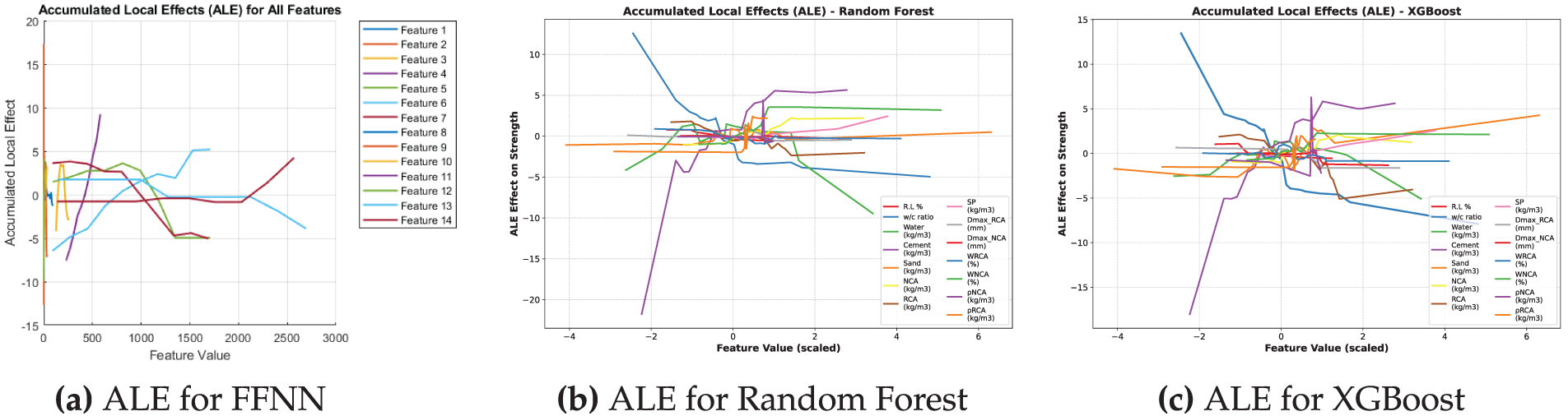
Figure 17: Comparison of ALE plots for different models

The addition of RAs has a nonlinear influence on CS, as shown by the PDP 16 and ALE 17 graphs. In particular, the model shows that when RAs are added up to a moderate replacement levels (RL%), CS increases, after which strength tends to decrease. This trend aligns with the experimental results presented by Khan et al. [60], who found that structural concrete applications can retain acceptable strength with 30%–40% RAs replacement. In a similar domain, Ali et al. [61] illustrated that high-strength concrete preserves its mechanical properties with up to 25%–30% RAs when enhanced with mineral admixtures. Furthermore, previous research conducted by Kumar and Rao [62] corroborated that replacing up to 20%–30% with RAs results in CS that is comparable to traditional mixes. Significantly, substituting NAs with RAs at a level of 30% has demonstrated a reduction in CO2 emissions by roughly 12%–20%, contingent upon regional sourcing and transportation considerations [61]. These findings indicate that the model successfully reflects behavior consistent with the domain, allowing engineers and material designers to estimate strength based on the properties of aggregates without the need for extensive laboratory evaluations. The capacity to predict performance while incorporating recycled materials enhances the significance of model for sustainable mix design, providing both mechanical dependability and measurable environmental advantages.

4  Conclusion

In this study, synthetic data generation and FFNNs were utilized to forecast the CS of RAC. Data augmentation increased the dataset points, ensuring that the synthetic data maintained similar statistical characteristics to the original dataset collected from literature. Hyperparameters such as the number of layers, neurons, and five different optimizers were optimized using a grid search technique, which is time-saving and outperforms traditional trial-and-error techniques. Among these, the Levenberg-Marquardt optimizer emerged as the best, yielding faster convergence and high forecasting accuracy. The optimized FFNN model with a three-hidden-layer structure (30-20-10 neurons) achieved strong performance with R = 0.9835, R2 = 0.9669, RMSE = 2.2127 MPa, and MAE = 0.873 MPa. Sensitivity analysis further identified cement and water content as the most influential parameters in predicting RAC strength. The PDP and ALE plots revealed nuanced relationships between input variables and model predictions, identifying the RCA component as a key driver of model behavior. Notably, the analysis showed that increasing the RCA content enhances concrete strength up to a certain threshold, beyond which further addition leads to a decline in strength–highlighting a non-linear effect that underscores the importance of optimal RCA dosage.

However, this study is limited by the simplified characterization of RAs, which excludes pretreatment effects, and does not account for the influence of supplementary cementitious materials (SCMs) or fine aggregate replacement factors that may significantly affect RAC performance in practical applications.

Subsequent research ought to broaden this methodology by integrating additional variables, including curing age, types of additives, and SCMs, which are essential for the performance of RAC. Given the environmental ramifications of cement, transfer learning with the same developed FFNN model can be implemented on SCM-based datasets, minimizing the need for collecting substantial new dataset with improved predictive accuracy and promoting sustainability through reduced CO2 emissions. This study demonstrates that synthetic data augmentation, when paired with optimized neural networks, offers an effective and flexible framework for predicting RAC compressive strength.

Acknowledgement: This work was supported and funded by the Deanship of Scientific Research at Imam Mohammad Ibn Saud Islamic University (IMSIU) (grant number IMSIU-DDRSP2503).

Funding Statement: This work was supported and funded by the Deanship of Scientific Research at Imam Mohammad Ibn Saud Islamic University (IMSIU) (grant number IMSIU-DDRSP2503).

Author Contributions: Sandeerah Choudhary: Conceptualization, methodology, original draft, simulation; Tallha Akram: Methodology, simulation, review, data curability; Qaisar Abbas: Review & editing, funding; Irshad Qureshi: Review & editing, supervision; Mutlaq B. Aldajani: Review & editing, funding; Hammad Salahuddin: Simulation, review & editing. All authors reviewed the results and approved the final version of the manuscript.

Availability of Data and Materials: The datasets generated or analyzed during the current study are available in the Google Drive repository at https://drive.google.com/drive/folders/1sBnxUfpPGW0mwIDbXqvrcwSwQ4ihAOhT, accessed on 12 October 2025.

Ethics Approval: This research did not involve human participants or animals. Ethical approval was therefore not required.

Conflicts of Interest: The authors declare no conflicts of interest to report regarding the present study.

References

1. Mohamed OA, Zuaiter HA, Jawa MM. Carbonation and chloride penetration resistance of sustainable structural concrete with alkali-activated and ordinary Portland cement binders: a critical review. Sustain Struct. 2025;5(2):000075. doi:10.54113/j.sust.2025.000075. [Google Scholar] [CrossRef]

2. Chowdhury JA, Islam MS, Islam MA, Al Bari MA, Debnath AK. Analysis of mechanical properties of fly ash and boiler slag integrated geopolymer composites. Sustain Struct. 2025;5(2):000073. doi:10.54113/j.sust.2025.000073. [Google Scholar] [CrossRef]

3. U S Geological Survey. Natural Aggregates Statistics and Information. [cited 2025 Oct 13]. Available from: https://www.usgs.gov/centers/national-minerals-information-center/natural-aggregates-statistics-and-information. [Google Scholar]

4. Ajayi S, Oyedele L, Akinade O, Bilal M, Owolabi H, Alaka H, et al. Reducing waste to landfill: a need for cultural change in the UK construction industry. J Build Eng (JOBE). 2016;5(1):185–93. doi:10.1016/j.jobe.2015.12.007. [Google Scholar] [CrossRef]

5. Hu Q, Liu R, Su P, Huang J, Peng Y. Construction and demolition waste generation prediction and spatiotemporal analysis: a case study in Sichuan, China. Environ Sci Pollut Res. 2023;30(14):41623–43. doi:10.1007/s11356-022-25062-6. [Google Scholar] [PubMed] [CrossRef]

6. Naderpour H, Rafiean AH, Fakharian P. Compressive strength prediction of environmentally friendly concrete using artificial neural networks. J Build Eng. 2018;16:213–9. doi:10.1016/j.jobe.2018.01.007. [Google Scholar] [CrossRef]

7. Tam VWY, Soomro M, Evangelista ACJ. A review of recycled aggregate in concrete applications (2000–2017). Construct Build Mat. 2018;172:272–92. doi:10.1016/j.conbuildmat.2018.03.240. [Google Scholar] [CrossRef]

8. Abdelfatah A, Tabsh S. Review of research on and implementation of recycled concrete aggregate in the GCC. Adv Civil Eng. 2011;2011:567924. doi:10.1155/2011/567924. [Google Scholar] [CrossRef]

9. Rodríguez C, Parra C, Casado G, Miñano I, Albaladejo F, Benito F, et al. The incorporation of construction and demolition wastes as recycled mixed aggregates in non-structural concrete precast pieces. J Cleaner Product. 2016;127:152–61. doi:10.1016/j.jclepro.2016.03.137. [Google Scholar] [CrossRef]

10. Gulati R, Bano S, Bano F, Singh S, Singh V. Compressive strength of concrete formulated with waste materials using neural networks. Asian J Civil Eng. 2024;25(6):4657–72. doi:10.1007/s42107-024-01071-3. [Google Scholar] [CrossRef]

11. Sathiparan N, Subramaniam DN. Optimizing fly ash and rice husk ash as cement replacements on the mechanical characteristics of pervious concrete. Sustain Struct. 2025;5(1):000065. doi:10.1080/10298436.2022.2075867. [Google Scholar] [CrossRef]

12. Zhang X, Akber MZ, Zheng W. Prediction of seven-day compressive strength of field concrete. Constr Build Mater. 2021;305(5):124604. doi:10.1016/j.conbuildmat.2021.124604. [Google Scholar] [CrossRef]

13. Liu K, Zou C, Zhang X, Yan J. Innovative prediction models for the frost durability of recycled aggregate concrete using soft computing methods. J Build Eng. 2021;34(1):101822. doi:10.1016/j.jobe.2020.101822. [Google Scholar] [CrossRef]

14. Bui Q-AT, Nguyen DD, Le HV, Pham BT, Prakash I. Prediction of shear bond strength of asphalt concrete pavement using machine learning models and grid search optimization technique. Comput Model Eng Sci. 2025;142(1):691–712. doi:10.32604/cmes.2024.054766. [Google Scholar] [CrossRef]

15. Tariq J, Hu K, Gillani STA, Chang H, Ashraf MW, Khan A. Enhancing the predictive accuracy of recycled aggregate concrete’s strength using machine learning and statistical approaches: a review. Asian J Civil Eng. 2025;26(1):21–46. doi:10.1007/s42107-024-01192-9. [Google Scholar] [CrossRef]

16. Zhang J, Huang Y, Aslani F, Ma G, Nener B. A hybrid intelligent system for designing optimal proportions of recycled aggregate concrete. J Clean Prod. 2020;273(3):122922. doi:10.1016/j.jclepro.2020.122922. [Google Scholar] [CrossRef]

17. Munir MJ, Kazmi SMS, Wu YF, Lin X, Ahmad MR. Development of novel design strength model for sustainable concrete columns: a new machine learning-based approach. J Clean Prod. 2022;357(8):131988. doi:10.1016/j.jclepro.2022.131988. [Google Scholar] [CrossRef]

18. Munir MJ, Kazmi SMS, Wu Y, Patnaikuni I. Influence of concrete strength on the stress-strain behavior of spirally confined recycled aggregate concrete. IOP Conf Ser Mat Sci Eng. 2020;829(1):012004. doi:10.1088/1757-899x/829/1/012004. [Google Scholar] [CrossRef]

19. Ly HB, Pham BT, Dao DV, Le VM, Le LM, Le TT. Improvement of ANFIS model for prediction of compressive strength of manufactured sand concrete. Appl Sci. 2019;9(18):3841. doi:10.3390/app9183841. [Google Scholar] [CrossRef]

20. Cheng MY, Chou JS, Roy AFV, Wu YW. High-performance concrete compressive strength prediction using time-weighted evolutionary fuzzy support vector machines inference model. Automat Construct. 2012;28(2):106–15. doi:10.1016/j.autcon.2012.07.004. [Google Scholar] [CrossRef]

21. Dantas ATA, Leite MB, de Jesus Nagahama K. Prediction of compressive strength of concrete containing construction and demolition waste using artificial neural networks. Construct Build Mat. 2013;38:717–22. doi:10.1016/j.conbuildmat.2012.09.026. [Google Scholar] [CrossRef]

22. Nguyen TA, Ly HB, Mai HVT, Tran VQ. Prediction of later-age concrete compressive strength using feedforward neural network. Adv Mater Sci Eng. 2020;2020(1):762. doi:10.1155/2020/9682740. [Google Scholar] [CrossRef]

23. Murphy KP. Machine learning: a probabilistic perspective. Cambridge, MA, USA: The MIT Press; 2012. [Google Scholar]

24. Aghabalaei Baghaei K, Hadigheh SA. FRP bar-to-concrete connection durability in diverse environmental exposures: an optimal machine learning approach to predicting bond strength. Structures. 2025;76:108988. doi:10.1016/j.istruc.2025.108988. [Google Scholar] [CrossRef]

25. Nguyen TD, Cherif R, Mahieux PY, Lux J, Aït-Mokhtar A, Bastidas-Arteaga E. Artificial intelligence algorithms for prediction and sensitivity analysis of mechanical properties of recycled aggregate concrete: a review. J Build Eng. 2023;66:105929. doi:10.1016/j.jobe.2023.105929. [Google Scholar] [CrossRef]

26. Xu J, Zhao X, Yu Y, Xie T, Yang G, Xue J. Parametric sensitivity analysis and modelling of mechanical properties of normal- and high-strength recycled aggregate concrete using grey theory, multiple nonlinear regression and artificial neural networks. Construct Build Mat. 2019;211:479–91. doi:10.1016/j.conbuildmat.2019.03.234. [Google Scholar] [CrossRef]

27. Haider SA, Naqvi SR, Akram T, Kamran M, Qadri NN. Modeling electrical properties for various geometries of antidots on a superconducting film. Appl Nanosci. 2017;7:933–45. doi:10.1007/s13204-017-0633-4. [Google Scholar] [CrossRef]

28. Naqvi SR, Akram T, Haider SA, Kamran M, Shahzad A, Khan W, et al. Precision modeling: application of metaheuristics on current-voltage curves of superconducting films. Electronics. 2018;7(8):138. doi:10.3390/electronics7080138. [Google Scholar] [CrossRef]

29. Chopra P, Sharma RK, Kumar M. Artificial neural networks for the prediction of compressive strength of concrete. Int J Appl Sci Eng. 2015;13:187–204. [Google Scholar]

30. Nunez I, Marani A, Flah M, Nehdi ML. Estimating compressive strength of modern concrete mixtures using computational intelligence: a systematic review. Constr Build Mater. 2021;310(1):125279. doi:10.1016/j.conbuildmat.2021.125279. [Google Scholar] [CrossRef]

31. Duan ZH, Kou SC, Poon CS. Prediction of compressive strength of recycled aggregate concrete using artificial neural networks. Constr Build Mater. 2013;40(1):1200–6. doi:10.1016/j.conbuildmat.2012.04.063. [Google Scholar] [CrossRef]

32. Duan ZH, Kou SC, Poon CS. Using artificial neural networks for predicting the elastic modulus of recycled aggregate concrete. Constr Build Mater. 2013;44(7):524–32. doi:10.1016/j.conbuildmat.2013.02.064. [Google Scholar] [CrossRef]

33. Gholampour A, Mansouri I, Kisi O, Ozbakkaloglu T. Evaluation of mechanical properties of concretes containing coarse recycled concrete aggregates using multivariate adaptive regression splines (MARSM5 model tree (M5Treeand least squares support vector regression (LSSVR) models. Neural Comput Appl. 2020;32(1):295–308. doi:10.1007/s00521-018-3630-y. [Google Scholar] [CrossRef]

34. Deng F, He Y, Zhou S, Yu Y, Cheng H, Wu X. Compressive strength prediction of recycled concrete based on deep learning. Constr Build Mater. 2018;175(7):562–9. doi:10.1016/j.conbuildmat.2018.04.169. [Google Scholar] [CrossRef]

35. Hammoudi A, Moussaceb K, Belebchouche C, Dahmoune F. Comparison of artificial neural network (ANN) and response surface methodology (RSM) prediction in compressive strength of recycled concrete aggregates. Constr Build Mater. 2019;209:425–36. doi:10.1016/j.conbuildmat.2019.03.119. [Google Scholar] [CrossRef]

36. Khan K, Ahmad W, Amin MN, Aslam F, Ahmad A, Al-Faiad MA. Comparison of prediction models based on machine learning for the compressive strength estimation of recycled aggregate concrete. Materials. 2022;15(10):3430. doi:10.3390/ma15103430. [Google Scholar] [PubMed] [CrossRef]

37. Li Z, Yoon J, Zhang R, Rajabipour F, Srubar WVIII, Dabo I, et al. Machine learning in concrete science: applications, challenges, and best practices. npj Comp Mater. 2022;8(1):127. doi:10.1038/s41524-022-00810-x. [Google Scholar] [CrossRef]

38. Nguyen HAT, Pham DH, Ahn Y. Effect of data augmentation using deep learning on predictive models for geopolymer compressive strength. Appl Sci. 2024;14(9):3601. doi:10.3390/app14093601. [Google Scholar] [CrossRef]

39. Yasuno T, Nakajima M, Sekiguchi T, Noda K, Aoyanagi K, Kato S. Synthetic image augmentation for damage region segmentation using conditional GAN with structure edge. arXiv:2005.08628. 2020. [Google Scholar]

40. Chen N, Zhao S, Gao Z, Wang D, Liu P, Oeser M, et al. Virtual mix design: prediction of compressive strength of concrete with industrial wastes using deep data augmentation. Constr Build Mater. 2022;323(5):126580. doi:10.1016/j.conbuildmat.2022.126580. [Google Scholar] [CrossRef]

41. Liu KH, Xie TY, Cai ZK, Chen GM, Zhao XY. Data-driven prediction and optimization of axial compressive strength for FRP-reinforced CFST columns using synthetic data augmentation. Eng Struct. 2024;300(5):117225. doi:10.1016/j.engstruct.2023.117225. [Google Scholar] [CrossRef]

42. Marani A, Jamali A, Nehdi ML. Predicting ultra-high-performance concrete compressive strength using tabular generative adversarial networks. Materials. 2020;13(21):4757. doi:10.3390/ma13214757. [Google Scholar] [PubMed] [CrossRef]

43. Abunassar N, Alas M, Ali SIA. Prediction of compressive strength in self-compacting concrete containing fly ash and silica fume using ANN and SVM. Arabian J Sci Eng. 2023;48(4):5171–84. doi:10.1007/s13369-022-07359-3. [Google Scholar] [CrossRef]

44. Güçlü U, van Gerven MA. Deep neural networks reveal a gradient in the complexity of neural representations across the ventral stream. J Neurosci. 2015;35(27):10005–14. doi:10.1523/jneurosci.5023-14.2015. [Google Scholar] [PubMed] [CrossRef]

45. Nguyen TH, Nguyen T, Truong TT, Doan DTV, Tran DH. Corrosion effect on bond behavior between rebar and concrete using Bayesian regularized feed-forward neural network. Structures. 2023;51(3):1525–38. doi:10.1016/j.istruc.2023.03.128. [Google Scholar] [CrossRef]

46. Kamran M, Haider SA, Akram T, Naqvi SR, He SK. Prediction of IV curves for a superconducting thin film using artificial neural networks. Superlatt Microstruct. 2016;95(1):88–94. doi:10.1016/j.spmi.2016.04.018. [Google Scholar] [CrossRef]

47. Demirtürk D, Mintemur Ö, Arslan A. Optimizing LightGBM and XGBoost algorithms for estimating compressive strength in high-performance concrete. Arab J Sci Eng. 2025;52(7):129657. doi:10.1007/s13369-025-10217-7. [Google Scholar] [CrossRef]

48. Mai HVT, Nguyen TA, Ly HB, Tran VQ. Prediction compressive strength of concrete containing GGBFS using random forest model. Adv Civil Eng. 2021;2021(1):6671448. doi:10.1155/2021/6671448. [Google Scholar] [CrossRef]

49. Paranhos RS, Cazacliu BG, Sampaio CH, Petter CO, Neto RO, Huchet F. A sorting method to value recycled concrete. J Cleaner Product. 2016;112:2249–58. doi:10.1016/j.jclepro.2015.10.021. [Google Scholar] [CrossRef]

50. Van Tran M, La H, Nguyen T. Hybrid machine learning for predicting hydration heat in pipe-cooled mass concrete structures. Constr Build Mater. 2025;481:141558. doi:10.1016/j.conbuildmat.2025.141558. [Google Scholar] [CrossRef]

51. Ogunsanya M, Isichei J, Desai S. Grid search hyperparameter tuning in additive manufacturing processes. Manufact Lett. 2023;35:1031–42. doi:10.1016/j.mfglet.2023.08.056. [Google Scholar] [CrossRef]

52. Prechelt L. Automatic early stopping using cross validation: quantifying the criteria. Neural Netw. 1998;11(4):761–7. doi:10.1016/s0893-6080(98)00010-0. [Google Scholar] [PubMed] [CrossRef]

53. Kim JH, Lee J. Efficient dataset collection for concrete crack detection with spatial-adaptive data augmentation. IEEE Access. 2023;11:121902–13. doi:10.1109/access.2023.3328243. [Google Scholar] [CrossRef]

54. Asteris P, Kolovos K. Self-compacting concrete strength prediction using surrogate models. Neural Comput Appl. 2019;31(Suppl 1):409–24. doi:10.1007/s00521-017-3007-7. [Google Scholar] [CrossRef]

55. Wang Z. Validation, robustness, and accuracy of perturbation-based sensitivity analysis methods for time-series deep learning models. arXiv:2401.16521. 2024. [Google Scholar]

56. Lexicon SP. Partial dependence plots; 2025 [Internet]. [cited 2025 Sep 24]. Available from: https://softwarepatternslexicon.com/machine-learning/model-validation-and-evaluation-patterns/advanced-evaluation-techniques/partial-dependence-plots/. [Google Scholar]

57. Molnar C, Freiesleben T, König G, Herbinger J, Reisinger T, Casalicchio G, et al. Relating the partial dependence plot and permutation feature importance to the data generating process. In: World Conference on Explainable Artificial Intelligence. Cham, Switzerland: Springer; 2023. p. 456–79. [Google Scholar]

58. Apley DW, Zhu J. Visualizing the effects of predictor variables in black box supervised learning models. J Royal Statist Soc Series B Statist Method. 2020;82(4):1059–86. doi:10.1111/rssb.12377. [Google Scholar] [CrossRef]

59. Hover KC. The influence of water on the performance of concrete. Constr Build Mater. 2011;25(7):3003–13. doi:10.1016/j.conbuildmat.2011.01.010. [Google Scholar] [CrossRef]

60. Khan M, Hussain A, Raza M. Studying the usability of recycled aggregate to produce new concrete. J Eng Appl Sci. 2024;74(1):1–12. [Google Scholar]

61. Ali S, Zhang Y, Mehmood T. Examining the influence of recycled aggregates on the fresh and mechanical characteristics of high-strength concrete. Sustainability. 2024;16(20):9052. doi:10.3390/su16209052. [Google Scholar] [CrossRef]

62. Kumar R, Rao P. Experimental study on strength behaviour of recycled aggregate concrete. Int J Eng Res Technol (IJERT). 2013;2(5):2278–0181. doi:10.17577/IJERTV2IS100045. [Google Scholar] [CrossRef]