A Multi-Grid, Single-Mesh Online Learning Framework for Stress-Constrained Topology Optimization Based on Isogeometric Formulation

1  Introduction

Structural topology optimization (TO) aims to find the optimal material distribution within a given design domain such that an objective function is minimized and constraints are satisfied [1]. Compared with size optimization and shape optimization, TO offers a greatly enlarged design space and consequently better design solutions. It is, however, the most challenging, as it deals with the creation of new geometries from scratch.

Most existing topology optimization (TO) methods implicitly represent structures using a fixed grid of pixels or voxels and employ the widespread finite element method (FEM) to evaluate objective functions and constraints. Despite their broad applicability, these grid-based, FEM-reliant approaches face certain limitations. For instance, the low-order continuity between neighboring finite elements [1]—illustrated in Fig. 1a—can significantly reduce computational accuracy, especially for stress-related metrics. This makes such methods less suitable for stress-constrained TO design. To address this, some studies have proposed using adaptive mesh refinement to improve the smoothness of structure boundaries and enhance stress calculations [2–4]. The main idea is to refine the mesh in regions where higher accuracy is needed and coarsen it elsewhere to improve computational efficiency. However, even with a refined mesh, the design is still represented as a pixel-based image with non-smooth boundaries, as shown in Fig. 1b. Beyond the issue of stress calculation, optimized designs often require additional post-processing to be compatible with computer-aided design (CAD) software for manufacturing, which can further compromise design quality.

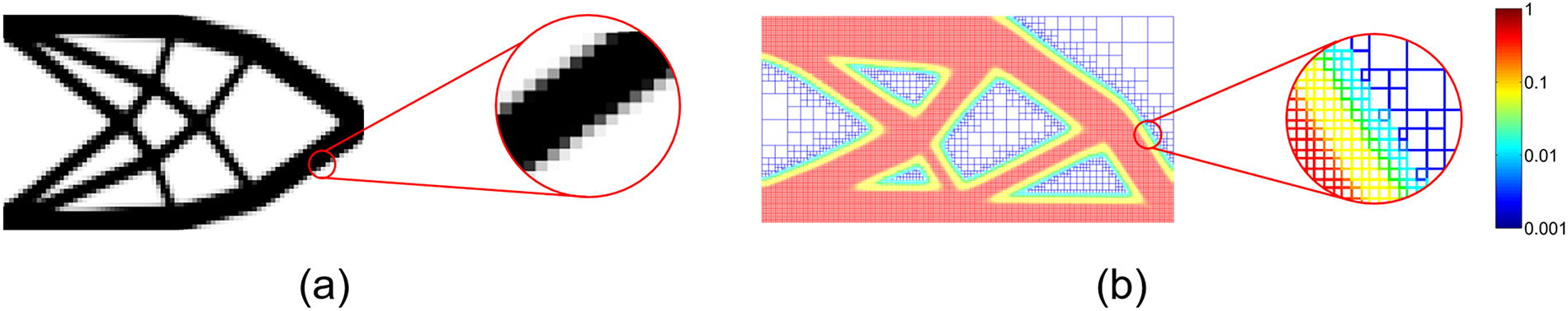
Figure 1: Optimized structure using (a) FEM-based TO [1], (b) FEM-based TO with adaptive mesh refinement [3]

To overcome the limitations of traditional FEM, Hughes and his co-workers [5,6] introduced the isogeometric analysis (IGA) framework, which unifies CAD and computer-aided engineering (CAE) by employing the same spline basis functions for both geometry representation and numerical analysis. This seamless integration eliminates the need for mesh generation and offers higher continuity and numerical accuracy compared to conventional FEM. All these advantages make IGA particularly advantageous for TO and form a new paradigm: isogeometric topology optimization (ITO). In particular, for stress-constrained design problems, the higher-order continuity of spline basis functions significantly enhances the accuracy of both structural representation and stress evaluation.

Significant efforts have been made to extend classical TO methods by incorporating IGA [7–9]. Representative examples include its integration with level-set [10], evolution method [11], and moving morphable component [12] approaches. Moreover, IGA has been combined with the boundary element method to tackle optimization problems in acoustics [13–15]. The density-based TO methods can be integrated with IGA by assigning design variables to the control points of the Non-uniform Rational B-splines (NURBS) basis function [16–19]. Stress-related ITO problems, typically believed to be more challenging due to factors such as the non-linear behavior of stress and the localized nature of stress constraints [20], have also been studied in recent years. For example, Kazemi et al. [21] proposed an ITO method for minimizing structural weight under local stress constraints using NURBS-based IGA, with control points’ density as design variables. The optimization process utilizes direct sensitivity analysis combined with the Method of Moving Asymptotes (MMA) for iterative updates [22]. To handle stress singularities, the ε relaxation method is employed. However, the optimized structures exhibit insufficient smoothness, likely due to the limited number of NURBS patches. Additionally, the reliance on direct sensitivity analysis (without using adjoint method) reduces efficiency for large-scale problems. Jahangiry and Tavakkoli [23] developed a level-set-based ITO method. The design variables are the control points of the NURBS-based level set function, which are iteratively updated by solving the Hamilton-Jacobi equation using the forward Euler scheme. Numerical examples, including weight minimization under local stress constraints and the simultaneous minimization of weight and strain energy, demonstrate the method’s capability to achieve reasonable results with smooth boundaries. Building on Gao’s work [17], Liu et al. [24] extended the SIMP-based IGA to tackle global stress-constrained TO problems. Density values at NURBS control points are used to construct the density distribution function, with a filter applied to ensure smoothness. The optimization problem is solved using MMA, while a global p-norm stress aggregation function constrains the stress during volume minimization. Numerical examples confirm that this approach can deliver smooth geometry representations and reliable stress analysis. To improve the optimization efficiency of Liu’s SIMP-based IGA work, Zhai [25] proposed a hybrid optimizer combining the alternating direction method of multipliers (ADMM) with MMA. Different from minimizing weight, Villalba et al. [26] focused on stress-constrained compliant mechanisms, using quadratic B-splines for material layout and structural analysis. By incorporating an overweight constraint to manage stress, their method achieves a 40%–60% reduction in computational time compared to classical FEM. In the monograph of Gao et al. [27], they studied the volume-constrained stress minimization problems in the ITO framework. Two global stress aggregation formulations (p-norm and Kreisselmeier-Steinhauser) are utilized to measure stress, which effectively eliminates boundary stress concentration issues. Vo et al. [28] integrated a gradient-free proportional topology optimization scheme into the isogeometric analysis framework, where NURBS basis functions simultaneously represent geometry, displacement, and material density. The approach defines densities at integration points in proportion to compliance, derives their relation to control points, and constructs a global NURBS-based density description.

Despite the significant development of ITO, the efficiency challenge remains and in fact becomes even more critical in large-scale stress-constrained TO designs. Compared with compliance design, stress-constrained TO is significantly more complex, often requiring many more iterations and longer convergence times. To address this, we extend a previously developed multi-grid, single-mesh online learning framework [29]—originally designed for compliance-based TO—to the ITO setting. This extension leverages the ITO framework’s inherent capacity for smooth geometric representation, enabling more accurate stress calculations.

The use of artificial neural network (ANN)-based surrogate models to accelerate topology optimization (TO) is an active field of research [30–34]. While various methods have been proposed, they often require large, expensive-to-generate training datasets. For applications involving only a few large-scale design problems, generating a large training dataset certainly is not efficient and sometimes even infeasible. For such cases, online learning presents another promising approach [35]. Unlike offline methods that rely on pre-collected datasets, online learning collects training data from designs and analysis results obtained during previous TO iterations. This eliminates the need for extensive upfront data generation and allows the neural networks to adapt specifically to the problem at hand, making online learning particularly well-suited for large-scale TO problems. To ensure accuracy, ANN models are continuously updated throughout the TO process as new training data is available. This iterative refinement ensures that the surrogate models remain closely aligned with the evolving design space, improving both computational efficiency and solution quality.

Online learning framework for TO was first proposed in [35] for compliance design. The method employs a localized patch-based prediction strategy to greatly enhance the scalability of the method and training data diversity. However, it neglects the structural information outside each local region when predicting patch responses. This may lead to an undetermined mapping and suboptimal prediction accuracy. Additionally, the coarse-fine two-grid mapping technique employed introduces additional computational overhead associated with generating coarse grid solutions. To overcome these limitations, our group recently developed a multigrid, single-mesh online learning TO method [29], which has demonstrated a better performance. In the present work, we further extend this advanced framework to stress-constrained design problems and validate its efficacy through a series of illustrative examples.

2  Isogeometric Analysis

2.1 NURBS Basis Functions

NURBS are widely employed in IGA and have become the primary technology for representing complex geometries in CAD software. To define a B-spline, a knot vector must be specified as an ordered sequence of increasing parameter values, denoted as Ξ={ξ1,ξ2,…,ξ𝓃+p+1},ξi≤ξi+1 where ξi is the ith knot, n is the number of basis functions and p is the polynomial order. A knot vector is termed uniform if the knots are spaced equally and non-uniform otherwise. The knot vector is open if the first and last knots appear with multiplicity p + 1. In this study, open knot vectors are used, which have become the standard in CAD practices [5].

For a given knot vector Ξ, the corresponding B-spline functions are recursively defined as follows:

Ni,p(ξ)=ξ−ξiξi+p−ξiNi,p−1(ξ)+ξi+p+1−ξξi+p+1−ξi+1Ni+1,p−1(ξ),(1)

where ξ is a parameter in the parametric domain. ξi are the values in the knot vector Ξ. The recursion starts with:

Ni,0(ξ)={1, if ξi≤ξ<ξi+10, otherwise ,(2)

where i=1,2,…,n is the basis function index.

Given two knot vectors for each parametric direction Ξ1={ξ1,ξ2,…,ξn+p+1} and Ξ2={η1,η2,…,ηn+p+1}, and n×m control points Pi,j, a B-spline surface is constructed as:

S(ξ,η)=∑i=1n∑j=1mNi,p(ξ)Nj,q(η)Pi,j,(3)

where Ni,p(ξ) and Nj,q(η) are the univariate basis functions of orders p and q, associated with knot vectors Ξ1 and Ξ2. The interval [ξi,ξi+1]×[ηi,ηi+1] is called knot spans in the parametric domain. Each control point Pi,j is a point in physical space, typically defined by its coordinates (x, y), that influences the shape of the surface locally. For any given pair of parametric coordinates (ξ,η), this equation computes the corresponding coordinates in the physical domain.

B-spline cannot represent certain shapes exactly, such as circles. Consequently, NURBS has become the de facto standard in CAD for handling more complex shapes [36]. Based on B-spline, a NURBS surface can be expressed as:

S(ξ,η)=∑i=1n∑j=1mRi,jp,q(ξ,η)Pi,j,(4)

where Ri,jp,q(ξ,η) represents the bivariate basis function defined as:

Ri,jp,q(ξ,η)=Ni,p(ξ)Nj,q(η)ωi,j∑k=1n∑l=1mNk,p(ξ)Nl,q(η)ωk,l,(5)

where ωi,j indicates the weights corresponding to the control point Pi,j. B-spline is a special case of NURBS where all weights are equal.

2.2 Isogeometric Structural Analysis

Using NURBS basis functions Ri,jp,q(ξ,η), the material (density) distribution function [17] across the 2D design domain can be represented as:

ρ(ξ,η)=∑i=1n∑j=1mRi,jp,q(ξ,η)ρi,j(6)

where ρi,j represents the pseudo-density (control density) variable associated with the control point Pi,j. This formulation establishes a mapping between the density variables and the material distribution. Due to the non-negativity and partition of unity properties of NURBS basis functions [36], it follows that 0≤ρ(ξ,η)≤1 if 0≤ρi,j≤1. When the density ρ at a point (ξ,η) is close to 0, it indicates an absence of material; conversely, if ρ is close to 1, the material is present at that location. Thus, the iso-surface of the ρ(ξ,η), typically with a default threshold of 0.5, is used to represent the structure.

In this study, the same NURBS basis functions are used to represent the displacement field in structural analysis. The displacement field can be defined as:

u(ξ,η)=∑i=1n∑j=1mRi,jp,q(ξ,η)ui,j(7)

where ui,j is the displacement vector associated to the control point Pi,j. For 2D examples, each control point has two independent displacement variables ui,jx and ui,jy.

In the IGA framework, elements are defined similarly to that in the FEM, with each IGA element corresponding to a knot span, denoted [ξi,ξi+1]×[ηi,ηi+1]. The system stiffness matrix is constructed by assembling local element stiffness matrices. The IGA elements in the parametric space divided by the knot vector are shown in Fig. 2a. After the mapping following Eq. (4), each parametric IGA element Ω^e corresponds to an element Ωe in the physical space, as shown in Fig. 2b. To facilitate computation, an affine mapping from the bi-unit parent element Ω~e to Ω^e in parametric space is defined, as illustrated in Fig. 2c. Here, J1 and J2 are Jacobi matrices of the two mappings. The element stiffness matrix in IGA is evaluated using Gauss quadrature, and in the physical domain, the stiffness matrix for element e is given by:

Ke=∫Ωe.BTDBdΩe=∫Ω~e.BTDB|J1||J2|dΩ~e,(8)

where B is the strain-displacement matrix derived from the partial derivatives of NURBS basis functions Ri,jp,q. D represents the elastic (constitutive) matrix, which can be expressed as:

D=E1−μ2[1μ0μ10001−μ2],(9)

where μ is the Poisson’s ratio and E is the modulus of elasticity. Based on the power-law relation, E can be expressed as E=ρ(ξ,η)γE0, where γ is the penalization parameter. The global stiffness matrix K is then assembled in a similar way as the standard finite elements process [5]:

K=∑Ke.(10)

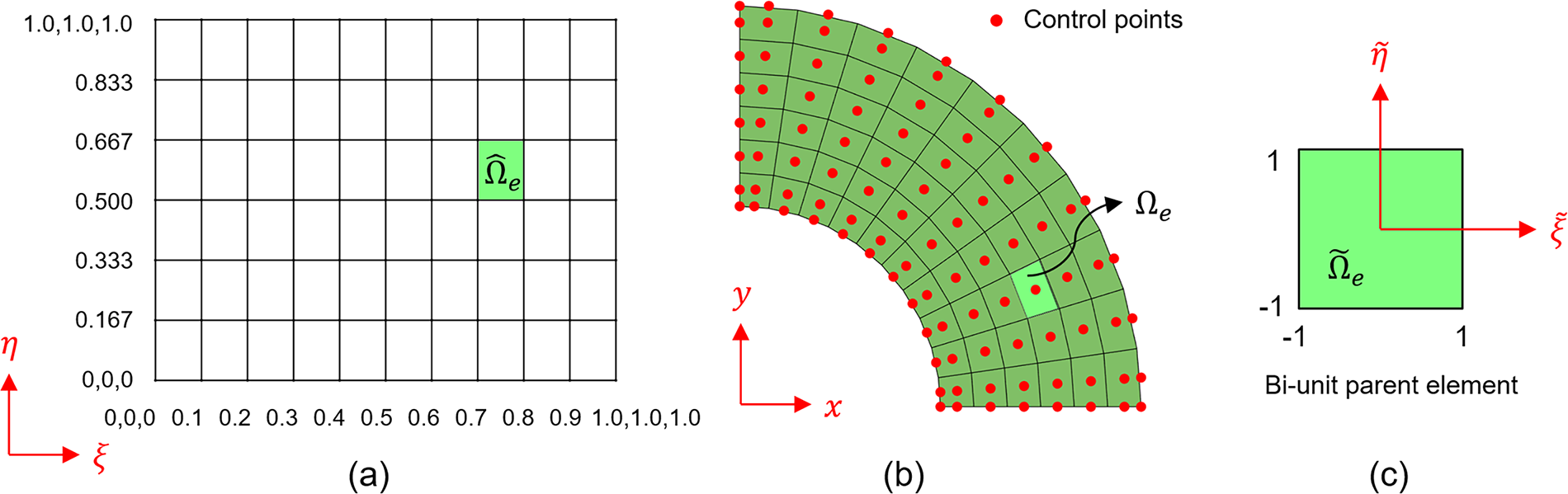
Figure 2: Schematic of an 2D element, Ω^e, in parametric space (a) and the corresponding 2D element Ωe in physical space (b). (c) The parent element Ω~e for integration. The knot vectors used in the schematic are Ξ1={0,0,0,0.1,0.2,…,0.9,1.0,1.0,1.0} and Ξ2={0,0,0,0.167,0.333,…,0.833,1.0,1.0,1.0}

Boundary conditions in IGA are implemented as follows [5]. Each control point is assigned to a load vector fi,j. For Neumann boundary conditions, the prescribed load values are assigned directly to the load vector fi,j. All fi,j are assembled in a similar way as FEM to form a global external load vector f. Dirichlet boundary conditions are applied by constraining the displacements ui,j of specific control points [17]. All ui,j are then assembled in a global displacement vector u. The global vector u is obtained by solving the global matrix:

Ku=f.(11)

Finally, the displacement ui,j for each control point can be determined from u. The entire displacement field across the structure can be derived using Eq. (7).

3  Stress-Constrained Design Problem

This section outlines the TO formulation of stress-constrained design problems based on IGA. The NURBS-based density distribution function is used to formulate the ITO approach, with IGA applied to compute structural responses. The Method of Moving Asymptotes (MMA) is employed to update design variables.

Nodal densities ρi,j associated with control points are defined as the design variables, which are evolved during optimization. A Shepard function [17] is utilized to filter the nodal densities, ensuring overall smoothness. The smoothed nodal density 𝒢i,j is expressed as:

𝒢i,j=∑l=1𝒩∑h=1ℳψ(ρl,h)ρi,j,(12)

where 𝒩 and ℳ are the numbers of control points within the local support area of the current control point. The Shepard function ψ(ρl,h) is defined as:

ψ(ρl,h)=w(ρl,h)∑l∗=1𝒩∑h∗=1ℳw(ρl∗,h∗),(13)

where w(ρl,h) is the weight function for the (l,h) nodal density, constructed using compactly supported radial basis functions [37] with C4 continuity:

w(ρl,h)=max(0,(1−r))6(35r2+18r+3),(14)

where r=d/dm. d is the Euclidean distance between the current (l,h) control point and another (i,j) control point. dm is the radius of the local support domain.

After filtering, a projection function [38] is applied to reduce intermediate density values:

𝓂(𝒢i,j)=tanh⁡(βη)+tanh⁡(β(𝒢i,j−η))tanh⁡(βη)+tanh⁡(β(1−η)),(15)

where η is the threshold (default: 0.5) and β is the shape control parameter.

Based on the projection function, m˙(𝒢i,j), the sensitivity of the projection function, is given by:

m˙(𝒢i,j)=∂𝓂(𝒢i,j)∂𝒢i,j=βsech(β(𝒢i,j−η))2tanh⁡(βη)+tanh⁡(β(1−η)).(16)

In isogeometric analysis, the knot vector discretizes the design domain into IGA elements. For the stress-constrained topology optimization problem studied in this work, a constant density distribution within each IGA element is employed for problem formulation and sensitivity calculations. The density at the centroid of an IGA element is chosen as the elemental relative density, ρe, which is calculated as:

ρe=∑i=1n∑j=1mRi,jp,q(ξec,ηec)𝓂(𝒢i,j),(17)

where (ξec,ηec) are the parametric coordinates of the eth element centroid. Based on the IGA discretization, the volume minimization problem with a maximum von Mises stress constraint is formulated as:

{infρ:J(ρ)=∑e=1Neρeves.t.:G(𝒳)=max(σavm)−σlim≤0 for a=1,2,…,Na,(18)

where J represents the structural volume. ve is the IGA element volume, and Ne is the number of IGA elements. σavm is the von Mises stress and σlim is the prescribed stress limit. Na is the total number of evaluation points. Typically, 2 × 2 Gauss points are employed for quadratic IGA elements. The elemental constitutive matrix is derived using a power-law relationship, De=ρeγD0, which is used to obtain the stiffness matrix.

The von Mises stress at a stress evaluation point a is expressed as:

σavm=(σaTVσa)0.5,(19)

where σa=ρesD0Baue is the stress vector. The parameter s is set to a recommended value of 0.5 [39]. Ba is the strain-displacemnet matrix. ue is the elemental displacement vector. V is the constant matrix defined as:

V=[1−0.50−0.510003].(20)

To alleviate the difficulty in the optimization caused by local stress constraint, a p-norm global stress measure is employed to approximate the local maximum stress:

G(𝒳)=c⋅σpn−σlim≤0,(21)

where σpn=(∑a=1Na(σavm)p)−p. Na is the total number of evaluation points. The scaling coefficient c is updated at each iteration as cn=max(σa,nvm)/σnpn to minimize the gap between the p-norm stress σnpn and the maximum stress, where subscript n refers to the iteration number.

Based on the adjoint method detailed in the next subsection, the sensitivity of the objective and the constraint are obtained and summarized as:

{∂J∂ρi,j=∑e∈Ii,jRi,jp,q⁡(ξec,ηec)⁢m˙⁡(Gi,j)⁢ψ⁡(ρi,j)⁢ve∂G∂ρi,j=c⁡∑a∈Ji,j(σp⁢n)1−p⋅(σav⁢m)p−2⁢VT⁢σa⁢s⁢ρes−1⁢Ri,jp,q⁡(ξec,ηec)⁢m˙⁡(Gi,j)⁢ψ⁡(ρi,j)⁢D0⁢Ba⁢ue−c⁡(λT⁢∂K∂ρi,j⁢u),(22)

where Ii,j is the set of elements connected to the control point Pi,j. Ji,j is the set of stress evaluation points associated with Pi,j. The adjoint vector λ is calculated by solving the following equation:

Kλ=∑a=1Na(σpn)1−p⋅(σavm)p−2(ρesD0Ba)TVTσa.(23)

The term ∂K/∂ρi,j in Eq. (22) is composed of the derivative of element stiffness matrix w.r.t. the design variable:

∂Ke∂ρi,j=∫Ωe.BTγρeγ−1Ri,jp,q(ξec,ηec)m˙(𝒢i,j)ψ(ρi,j)D0BdΩe.(24)

After obtaining the sensitivity, the MMA optimizer [22] is used to update the control density ρi,j. To improve the numerical stability of the topology optimization process, several schemes are employed. The coefficient c is averaged over the last 4 iterations, which means at the nth iteration, it is calculated as cn=0.25(cn+cn−1+cn−2+cn−3). The design variable ρ is also updated based on the average value: ρn=0.5(ρn+ρn−1). In the power law relationship to obtain the elemental constitutive matrix, γ starts at 0.8 and increases by 0.2 per iteration until reaching a maximum of 3.

Sensitivity Analysis

Based on the IGA discretization, the volume minimization problem with a maximum von Mises stress constraint is formulated in Eq. (18). The sensitivity of the objective function J and constraint G to the design variable ρi,j are detailed in this subsection.

First, the derivative of objective J w.r.t. the ρi,j can be expressed as:

∂J∂ρi,j=∑e=1Ne∂ρe∂ρi,jve.(25)

Since the density at the centroid of an IGA element is chosen as the elemental relative density, ρe, which is given by:

ρe=∑i=1n∑j=1mRi,jp,q(ξec,ηec)m(𝒢i,j),(26)

where (ξec,ηec) is the parametric coordinate of the eth element centroid. Substituting Eqs. (26) into (25), we derive:

∂J∂ρi,j=∑e∈Ii,jRi,jp,q(ξec,ηec)∂m(𝒢i,j)∂ρi,jve,(27)

where Ii,j is the set of elements connected to the control point Pi,j. Incorporating the formulation of projection function in Eq. (15) and filter function in Eq. (13), the (27) becomes:

∂J∂ρi,j=∑e∈Ii,jRi,jp,q(ξec,ηec)m˙(𝒢i,j)ψ(ρi,j)ve,(28)

where m˙(𝒢i,j), the sensitivity of the projection function, is given by Eq. (16).

Next, the derivative of objective G w.r.t. the ρi,j is derived. Since we use p-norm stress σ~pn=c⋅σpn to approximate the max(σavm), we have:

∂G∂ρi,j=c∑a=1Na∂σpn∂σavm(∂σavm∂σa)T∂σa∂ρi,j.(29)

The intermediate terms are as follows:

∂σpn∂σavm=(σpn)1−p⋅(σavm)p−1.(30)

∂σavm∂σa=1σavmσaTV.(31)

Since σa=ρesD0Baue, the last term ∂σa/∂ρi,j in Eq. (29) becomes:

∂σa∂ρi,j=∂ρes∂ρi,jD0Baue+ρesD0Ba∂u∂ρi,j=sρes−1Ri,jp,q(ξec,ηec)m˙(𝒢i,j)ψ(ρi,j)D0Baue+ρesD0Ba∂u∂ρi,j.(32)

Substituting Eqs. (32) into (29) yields:

∂G∂ρi,j=c∑a=1Na∂σpn∂σavm(∂σavm∂σa)T(sρes−1Ri,jp,q(ξec,ηec)m˙(𝒢i,j)ψ(ρi,j)D0Baue+ρesD0Ba∂u∂ρi,j).(33)

Since external load is a constant, ∂f/∂ρi,j=0. By differentiating Ku=f, we have:

∂K∂ρi,ju+K∂u∂ρi,j=0.(34)

Multiplying Eq. (34) by λT and substituting into Eq. (33), we obtain:

∂G∂ρi,j=c∑a=1Na∂σpn∂σavm(∂σavm∂σa)T(sρes−1Ri,jp,q(ξec,ηec)m˙(𝒢i,j)ψ(ρi,j)D0Baue+ρesD0Ba∂u∂ρi,j)−λT∂K∂ρi,ju−λTK∂u∂ρi,j.(35)

Collecting all terms related to ∂u/∂ρi,j and let it equal to 0, we derive the adjoint equation:

Kλ=∑a=1Na∂σpn∂σavm(ρesD0Ba)T∂σavm∂σa=∑a=1Na(σpn)1−p⋅(σavm)p−2(ρesD0Ba)TVTσa.(36)

Solving Eq. (36) and substituting λ back to Eq. (35) gives the final expression:

∂G∂ρi,j=c∑a∈Ji,j∂σpn∂σavm(∂σavm∂σa)Tsρes−1Ri,jp,q(ξec,ηec)m˙(𝒢i,j)ψ(ρi,j)D0Baue−cλT∂K∂ρi,ju=c∑a∈Ji,j(σpn)1−p⋅(σavm)p−2VTσasρes−1Ri,jp,q(ξec,ηec)m˙(𝒢i,j)ψ(ρi,j)D0Baue−cλT∂K∂ρi,ju,(37)

where Ji,j is the set of stress evaluation points associated with Pi,j. The term ∂K/∂ρi,j in Eq. (37) is composed of the derivative of element stiffness matrix w.r.t. the design variable:

∂Ke∂ρi,j=∫Ωe.BTγρeγ−1Ri,jp,q(ξec,ηec)m˙(𝒢i,j)ψ(ρi,j)D0BdΩe.(38)

4  Online Learning Framework

The most time-consuming step in the IGA process is the calculation of the sensitivities ∂G/∂ρi,j, which depend on state variables. To speedup this calculation, the proposed online learning framework based on FNO model is employed to perform this sensitivity calculation. In this framework, design variables are the control densities, and an FNO surrogate model is constructed to predict sensitivity fields in selected iterations, replacing the conventional IGA calculations. The training data is collected dynamically using the design results obtained from previous TO iterations, and the FNO model is continuously updated using the newly generated data during the TO process.

The flowchart of the online learning process is shown in Fig. 3. During the initialization phase, the traditional TO process based on isogeometric analysis (TO-IGA) is conducted for n0 iterations. It is followed by another n1 TO-IGA iterations. The designs and analysis results generated during these n1 iterations are saved and used to train the initial FNO model. This initial FNO model is then integrated with TO process (TO-FNO) and optimization is carried out for n2 iterations. If the design is unsatisfactory, another n1 TO-IGA iterations are executed, and results generated from this process are collected. The optimized design at the last iteration is then evaluated. If it is still unsatisfactory, the FNO model is re-trained using the newly collected data, and the TO-FNO process continues for another n2 iterations. This alternative process between TO-IGA and TO-FNO continues until the design meets the specified objectives and constraints.

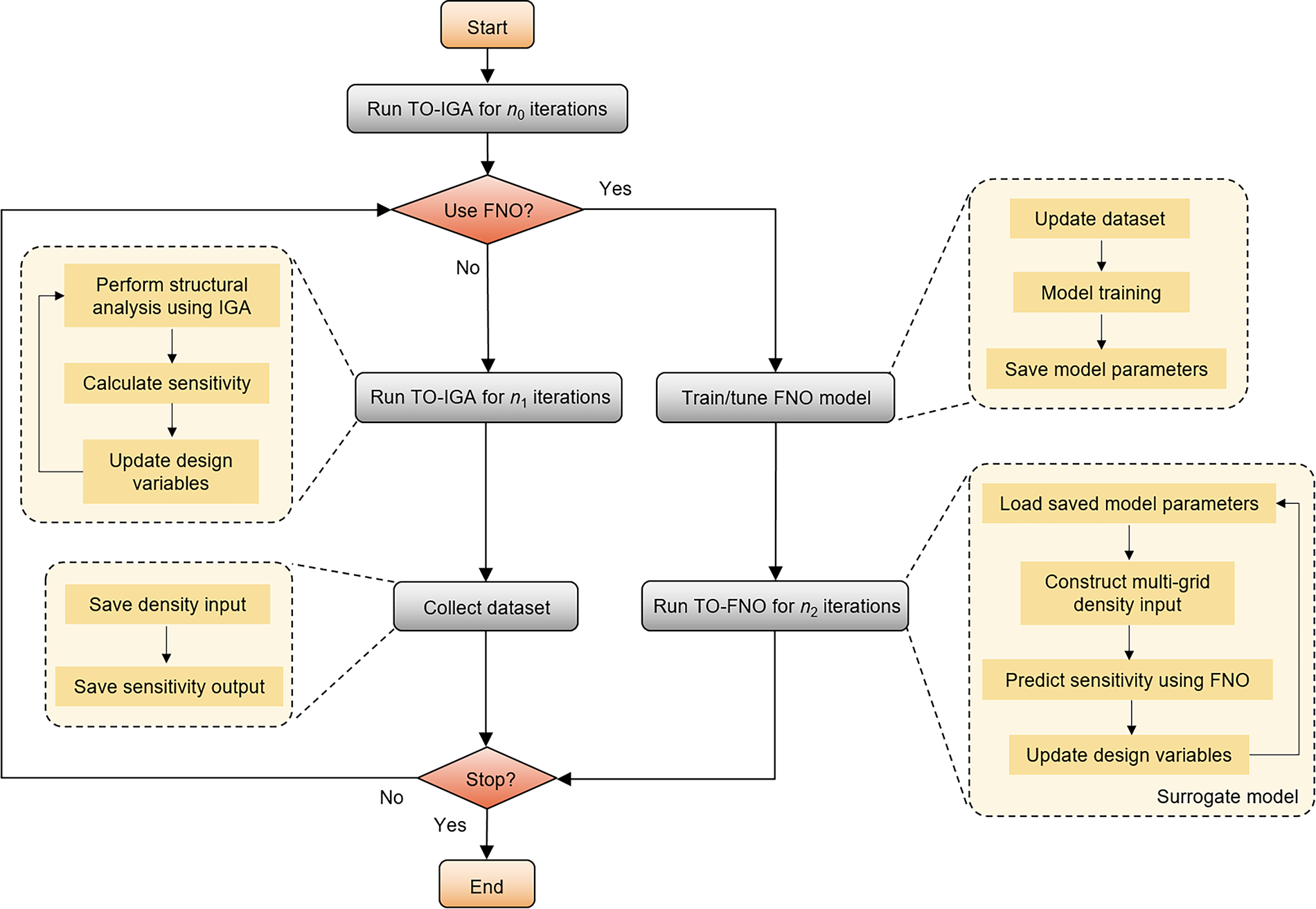
Figure 3: The flowchart of the proposed online learning framework based on the IGA and FNO surrogate model

4.1 FNO Surrogate Model

In this work, the FNO [40] is employed to construct a surrogate model that maps the control density ρ∈Rm×n of the design domain, generated during the TO process, to its corresponding sensitivity field. In the framework, we adopt a localized patch-based prediction and multi-grid decomposition strategy.

The architecture of the FNO and the multi-grid input of the density field are illustrated in Fig. 4. In this case shown in the figure, the MG level is 1, comprising two resolution levels (level 0 and level 1). The optimized structure is represented by density in physical space, however, the control density sorted in parametric space is selected as the input of FNO. The input tensor can be expressed as a∈Rb×c×m×n, where b is the batch size and c is the channel dimension, undergoes multi-grid decomposition along its spatial dimensions. This transformation yields an expanded tensor a∈R4b×2c×m/2×n/2, effectively increases the data volume by a factor of 4. This expansion proves particularly advantageous in online learning where training data may be limited. Following the multi-grid decomposition, the processed input is fed into the FNO model, which predicts the sensitivity field for each local region. These local predictions are then systematically concatenated to reconstruct the complete sensitivity field across the entire domain, as demonstrated in the rightmost portion of Fig. 4.

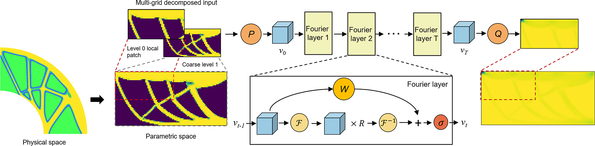
Figure 4: The architecture of multi-grid FNO. Left column: multi-grid density input with MG level of 1; Middle column: the architecture of the FNO; Right column: the predicted sensitivity

The iterative updating process v0⟼v1⟼…⟼vT of the FNO model is illustrated in the middle column of Fig. 4. First, the input a(x) is lifted to a high-dimensional representation v0=𝒫(a(x)) through a linear transformation 𝒫. This high-dimensional representation is then gone through a series of updates: vt⟼vt+1, t=0,1,⋯,T−1. Finally, it is projected back to the physical solution through a linear transformation Q: u(x)=Q(vT(x)). In the FNO training process, the control density ρ∈Rm×n is treated as input, which reflects the topology of the structure and is initially set to 0.5.

The updating formula for the latent representation is illustrated in Eq. (39). The key idea in this updating formula is to add a non-local integral operation to the usual network updating procedure in each hidden layer:

vt+1(x)=σ(Wtvt+(𝒦(a;ϕ)vt)(x)),∀x∈D,(39)

where W and σ stand for a linear transformation and non-linear activation function, a represents problem parameters, 𝒦 is a non-local integral operator defined as (𝒦(a;ϕ)vt)(x)=∫Dκϕ(x−y,a)vt(y)dy and ϕ denotes the network parameters. The operator 𝒦 is applied on function vt, which itself takes x as input. Therefore, the nested parentheses in Eq. (39) reflect the operator acting on a function evaluated at a point. The convolutional nature of the integral allows it to be computed via a fast Fourier transform as shown in the following equation.

(𝒦(a;ϕ)vt)(x)=ℱ−1(ℱ(κϕ)⋅ℱ(vt))(x)=ℱ−1(Rϕ⋅(ℱvt))(x),(40)

where ℱ denotes the Fourier transform of a function and ℱ−1 is its inverse. Rϕ is a tensor containing the Fourier coefficients of the kernel function κϕ, which is determined through learning via network updates. The detailed implementation can be found in Refs. [40,41].

4.2 Multi-Grid Input

The multi-grid decomposition approach adopted in this work builds upon the method presented in [42] and is designed for a domain D discretized into 2s1×2s2 elements, where s1,s2∈Z+. The procedure unfolds as follows:

•   Initial configuration:

–   If any domain edge is shorter than 2s1 or 2s2, padding is applied along that boundary to ensure compatibility.

–   At a target resolution level L, the domain D is uniformly divided into 22L non-overlapping regions Dj0 (level 0), each of size 2s1−L×2s2−L.

•   Hierarchical context expansion (levels k = 1 to L):

–   For each region Dj0, a sequence of larger surrounding regions Djk is defined. Each of Djk is centered on Dj0 and spans 2s1−L+k×2s2−L+k.

–   If these expanded regions extend beyond the domain boundaries, they are truncated accordingly.

–   Each region Djk is then uniformly downsampled by a factor of 0.5k in both directions, resulting in a patch of consistent size 2s1−L×2s2−L, matching the level 0 resolution.

•   Final output construction:

–   The downsampled patches from all levels (from 0 to L) are concatenated along the feature dimension to form a multi-grid input representation.

Fig. 5 demonstrates the hierarchical decomposition when the maximum level is set to 2. The base region at level 0 (green square) is first identified within the domain. Around this region, increasingly larger patches are defined at coarse levels 1 and 2. At each level, the corresponding patch is downsampled to match the resolution of the level-0 patch, maintaining a consistent size across all levels. The final MG input is constructed by concatenating the level 0 patch with its coarse-level counterparts, forming a multi-scale feature representation that captures both local detail and broader contextual information.

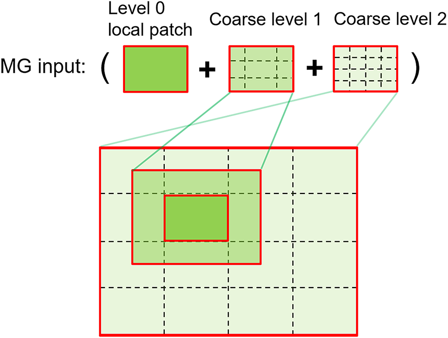
Figure 5: An illustration of the multi-grid input construction with MG level of 2

To enhance dataset richness, an overlapping scheme is applied to local regions. For each local patch of size W×H, neighboring patches are allowed to overlap by η1W and η2H in the horizontal and vertical directions, respectively. Here η1 and η2 denote the overlapping ratios. As illustrated in Fig. 6, when both overlapping ratios are set to 0.5, this configuration yields nine local patches at level 0: four core patches without overlap and five additional patches formed from overlapping regions.

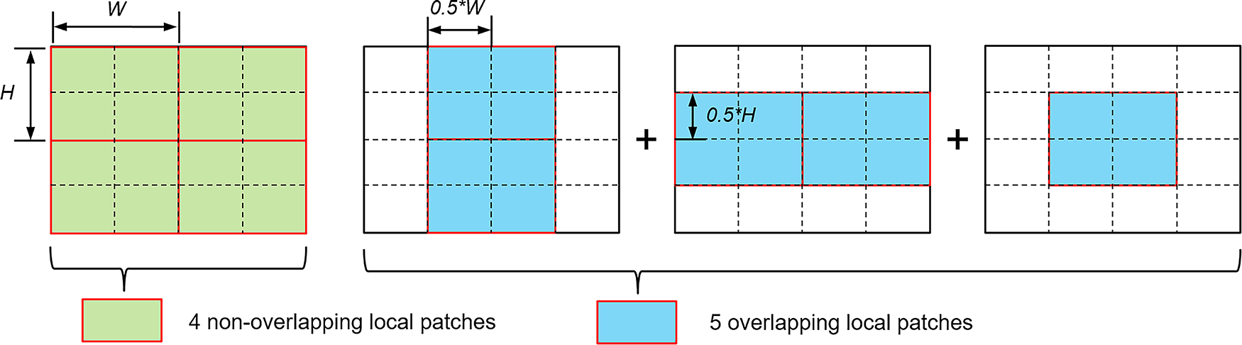
Figure 6: Illustration of the overlapping strategy with the overlapping ratio of 0.5 in both directions

5  Numerical Experiments

Two L-bracket design problems with different load positions, with their problem setups illustrated in Fig. 7, are used as the benchmark examples to validate the effectiveness of the online learning framework. The optimization parameters are set as follows. The filter radius is 4, which means the adjacent 4 control densities are used for smoothing. The default norm value for the p-norm is 8. In this work, a uniformly distributed load t is applied. To compute the load assigned to the control points, numerical integration is performed using five Gaussian quadrature points [17]. For example, in Fig. 7a, the load position in parametric space is ξ=[0.95,1.0],η=1.0. Load applied on control points (i,j) is calculated as:

Fi,j=∫0.951.0Ri,j(ξ,η)t(ξ,η)‖dS(ξ,η)dξ‖dξ≈∑k=1nRi,j(ξk)t(ξk)‖dS(ξk)dξ‖wk(41)

where t is the load per unit length, ξk and wk are the kth Gauss points location and weight within the interval [0.95, 1.0]. Each design problem considered a total load of 2.0 N, and the stress constraint limit is set at 25 Pa.

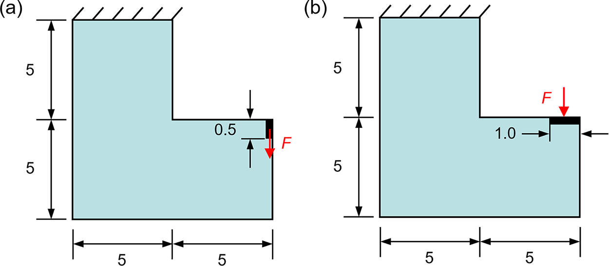
Figure 7: Design domain of the L-bracket for the stress-constrained design: (a) load applied at the top, and (b) load applied on the side

We also consider another design domain of quarter annulus, illustrated as Fig. 8. A total load of 2.0 N, and the stress constraint limit is set at 40 Pa.

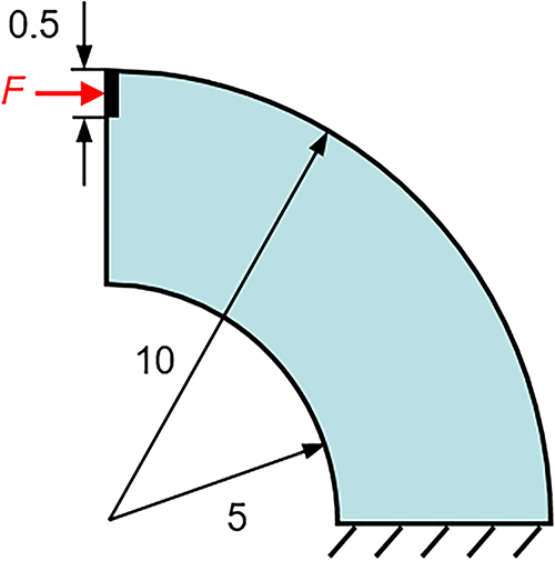
Figure 8: Design domain of the quarter annulus for the stress-constrained design

All numerical experiments are conducted on a Windows 10 Pro operating system with an i7-11700 CPU, 16 GB RAM, and an NVIDIA 3060 GPU with 12 GB RAM. The implementation was done in MATLAB 2020b, with the online learning component executed using Python 3.8 and PyTorch 1.10.2 framework. In the FNO model, the number of modes kept after the Fourier transform is 12. The channel width is 64 after the lifting layer.

5.1 Stress-Constrained Design Results

During the online learning process, the n1 and n2 values are maintained at 10 and 5, with optimization stopping after 210 iterations or the average change of the design variable smaller than 1e−3. The default multi-grid level is 1 with no overlap. Training or tuning is performed for 150 epochs using a batch size of 12. The number of obtained control points is 103 × 52, so we use bottom edge padding to get input with a size of 104 × 52. In the projection Eq. (15), β is initialized at 1.0 and increased by 1 every 10 iterations until reaching a maximum of 10. Data collection for online learning begins after the first 20 iterations (n0 = 20).

For the design problem described in Fig. 7a, based on our online learning framework, the structural evolution and the corresponding von Mises stress distributions at different iterations are shown in Fig. 9. The stress plots are generated from a point cloud. Each point corresponds to a Gauss point and is colored by its computed stress value. The results illustrate that the structure gradually converges to an optimized design.

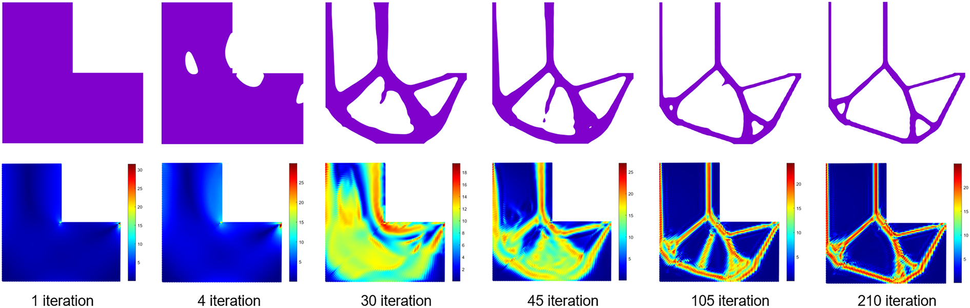
Figure 9: Design evolution and von Mises stress distribution at different iterations for the L-bracket example illustrated in Fig. 7a

Design results for both design problems are listed in Table 1, showing that the proposed online learning framework achieves results comparable to the ground truth TO-IGA in terms of the volume fraction value and stress constraint satisfaction. The effectiveness of the framework is validated by these findings. The evolution curves of volume fraction and the maximum von Mises stress are plotted in Fig. 10, indicating that the curve of the maximum von Mises stress obtained from the online learning process is less smooth than that of the ground truth TO-IGA due to discrepancies between FNO-predicted sensitivities and actual values. These differences occasionally cause localized increases in stress, which are corrected in subsequent IGA updates. As the optimization converges, the maximum stress stabilizes and basically meets the constraints. At the same time, the online learning method can reduce the number of IGA evaluations from 210 to 150, reducing the total computational time by about 20%.

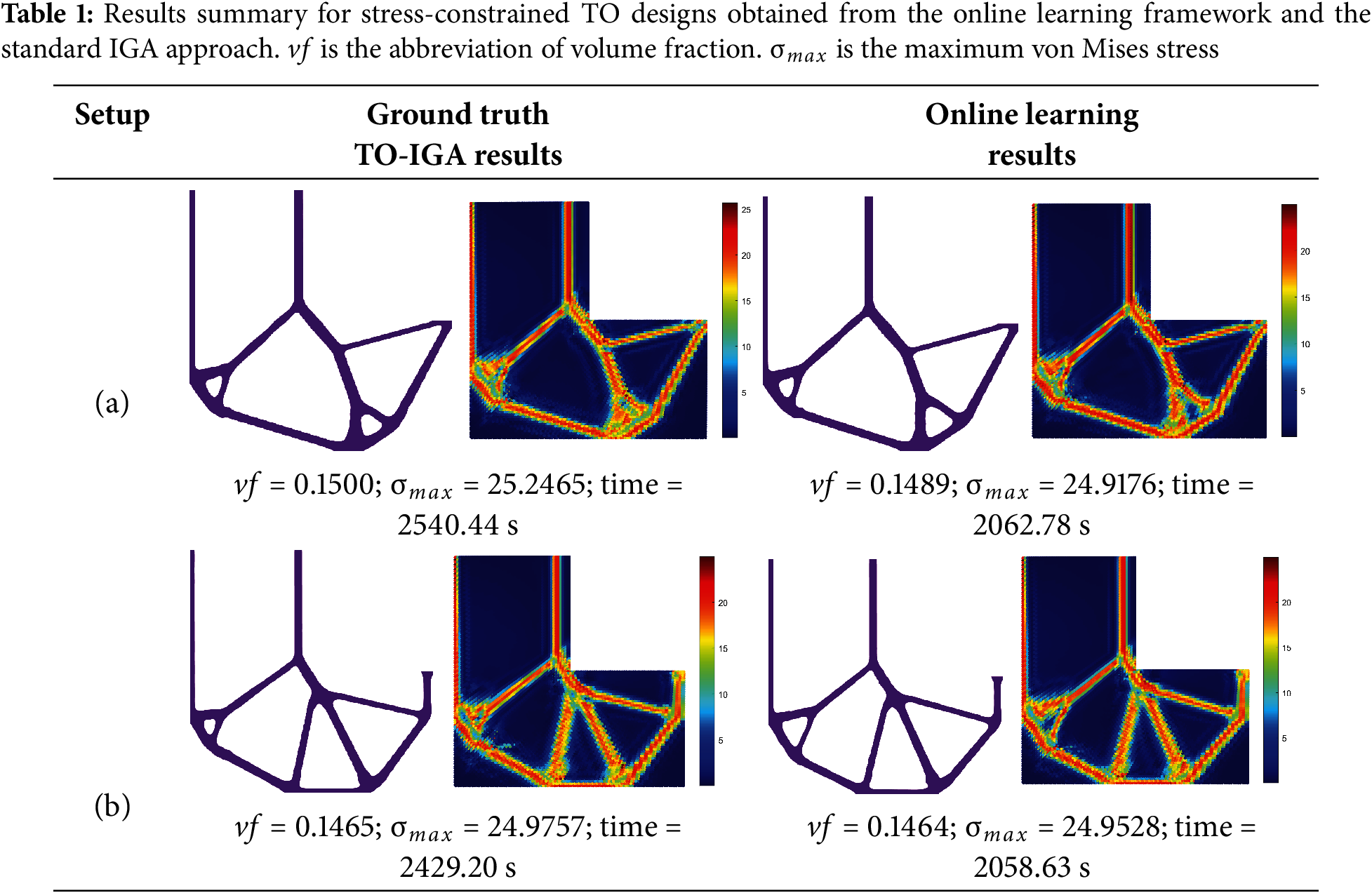
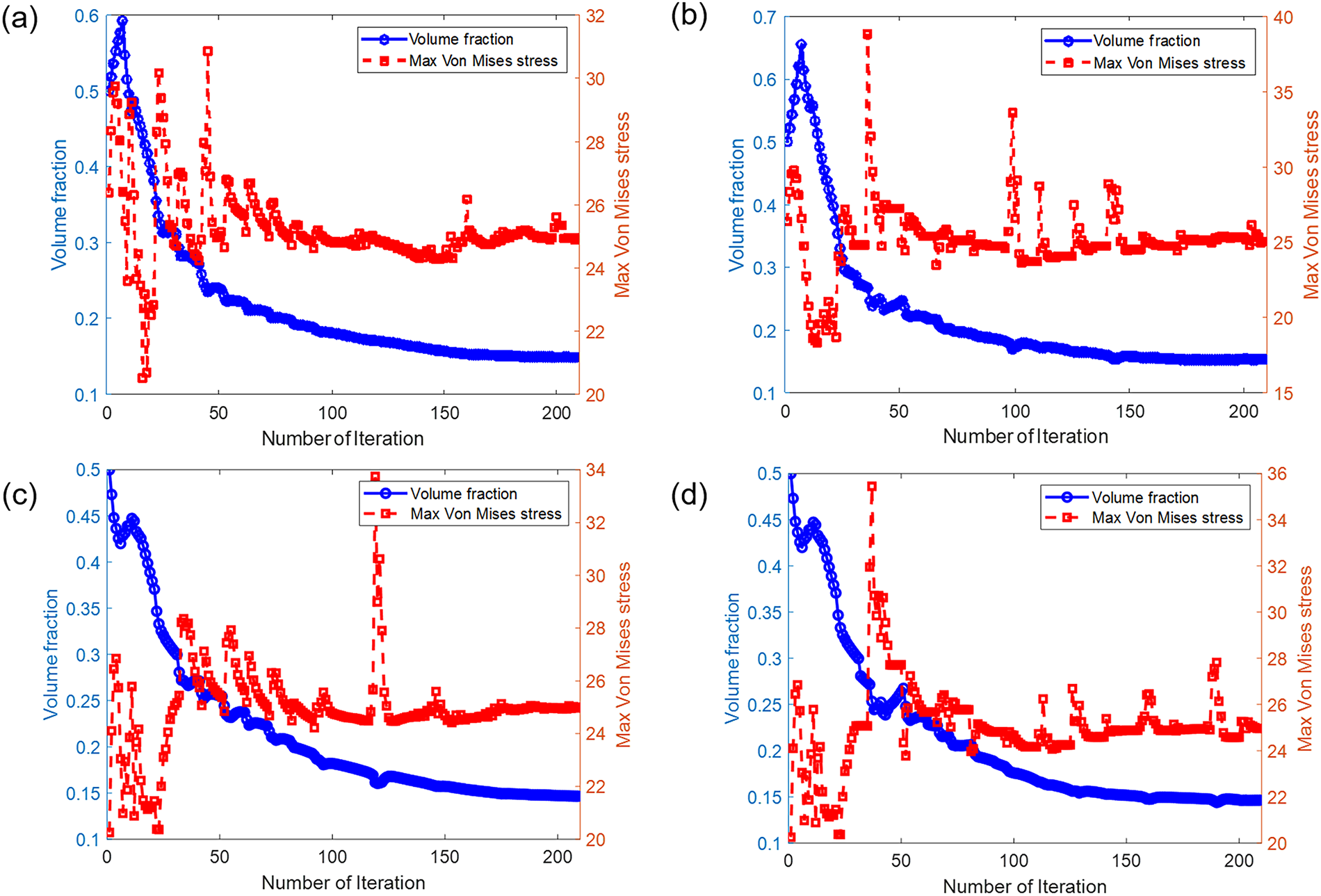
Figure 10: Volume fraction and maximum von Mises stress evolution curves of (a) ground truth result for the design problem shown in Fig. 7a, (b) online learning result for the design problem shown in Fig. 7a setup, (c) ground truth result for the design problem shown in Fig. 7b, (d) online learning result for the design problem shown in Fig. 7b

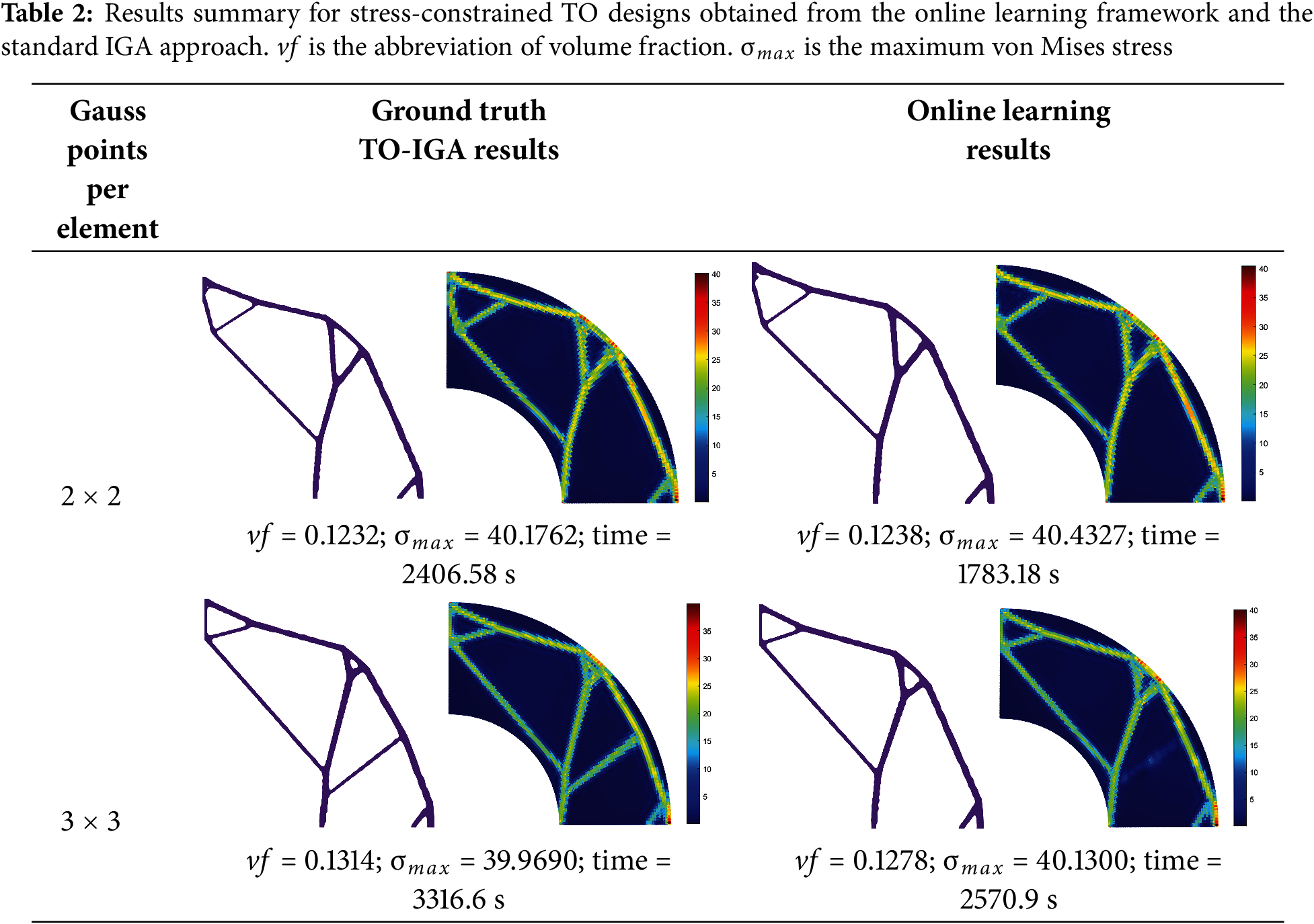
Under the same online learning parameter settings, the design results for the quarter annulus example are summarized in Table 2. We employ two different numbers of Gauss points to assess their influence. Increasing the number of Gauss points improves the accuracy of the response evaluation, leading to slight variations in the final optimized designs. Using a larger number of Gauss points also increases the total solving time. Nevertheless, under both settings, the online learning method consistently produces designs that are comparable to the ground truth, further confirming its effectiveness across different examples.

The evolution curves of volume fraction and the maximum von Mises stress using different Gauss points are plotted in Fig. 11. Convergence of the curves is observed with the increasing iteration count in the quarter-annulus example.

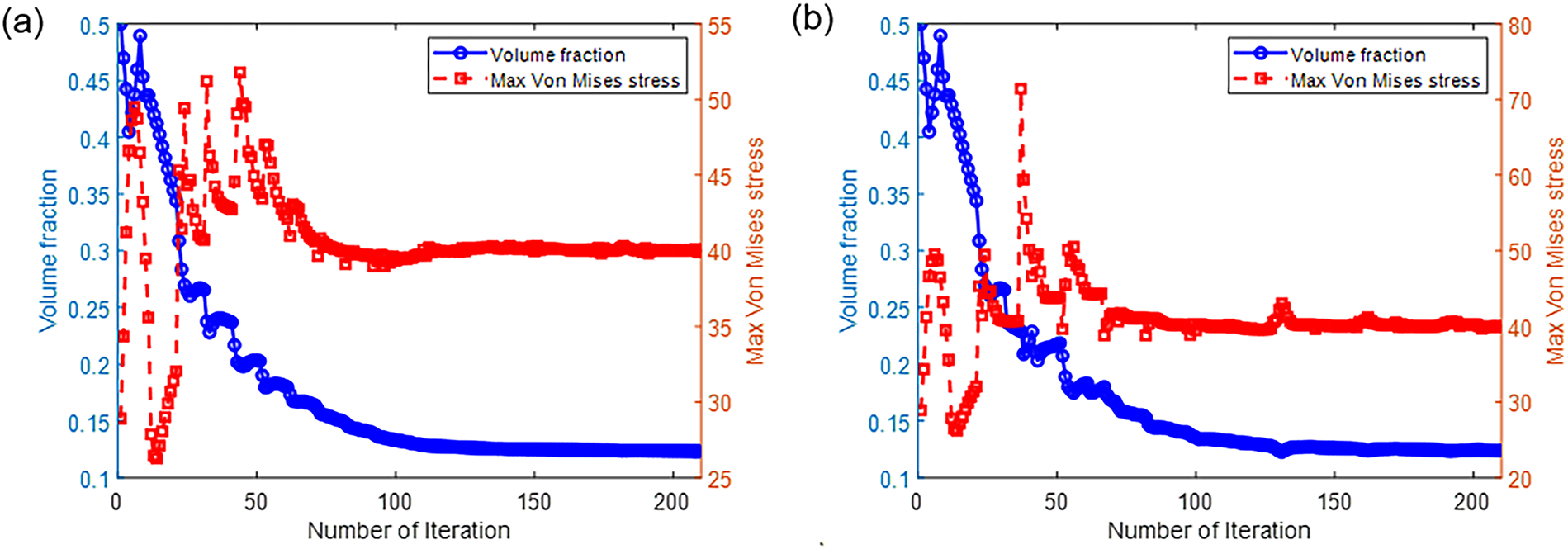
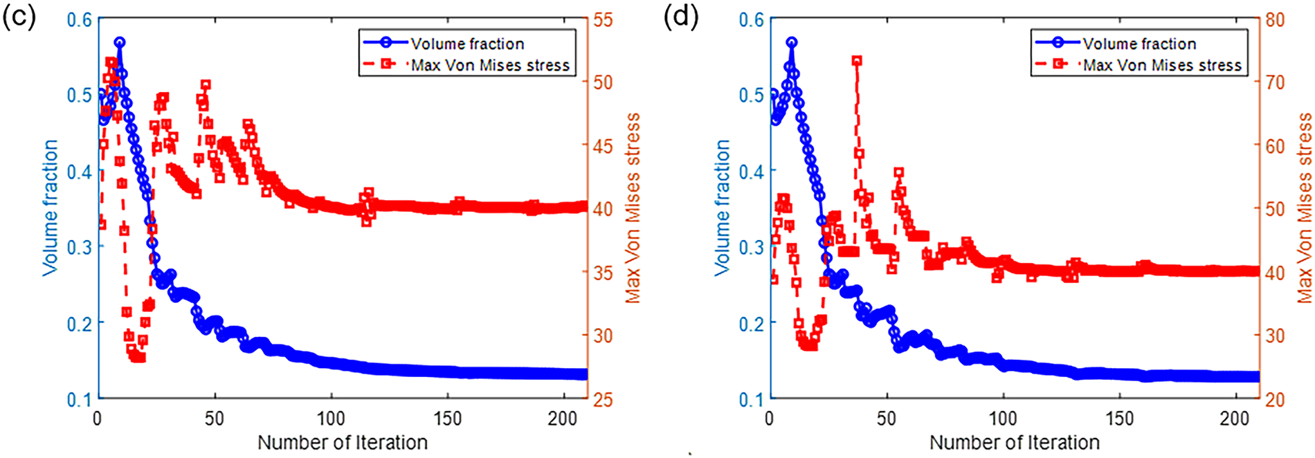
Figure 11: Volume fraction and maximum von Mises stress evolution curves of (a) ground truth result using 2 × 2 Gauss points for the design problem shown in Fig. 8, (b) online learning result using 2 × 2 Gauss points for the design problem shown in Fig. 8 setup. (c) ground truth result using 3 × 3 Gauss points for the design problem shown in Fig. 8, (d) online learning result using 3 × 3 Gauss points for the design problem shown in the setup of Fig. 8

5.2 Parameter Study

5.2.1 P-Norm

In this study, we employ p-norm stress as an approximation for maximum stress. The parameter p plays a crucial role in determining the approximation accuracy. To investigate the influence of the p-norm parameter on stress-constrained optimization, we test p-norm values of 4, 6, 8, and 10. The online learning settings are the same as those stated in Section 5.1, with results shown in Fig. 12. When p is too small, the optimized designs exhibit sharp corners. This phenomenon occurs because smaller values of p result in less accurate p-norm approximations of the maximum stress. As a result, the maximum stress of the optimized structure is slightly higher than those optimized structures obtained with a larger p value. For p>6, the objective function values are close to each other, and further increases in p have a negligible impact on the performance of the design. In addition, a very large p value, such as 10, may lead to numerical instability. Therefore, a default value of 8 is adopted in this work.

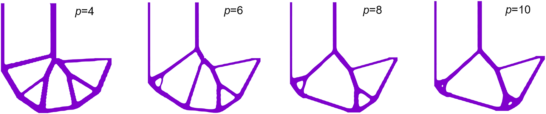
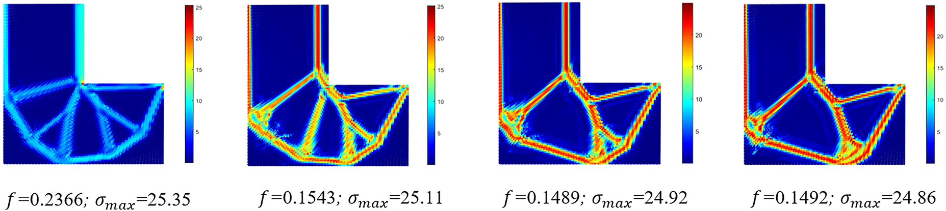
Figure 12: Online learning optimization results for different p-norm values. f is the volume objective. σmax is the maximum von Mises stress

5.2.2 Fourier Mode

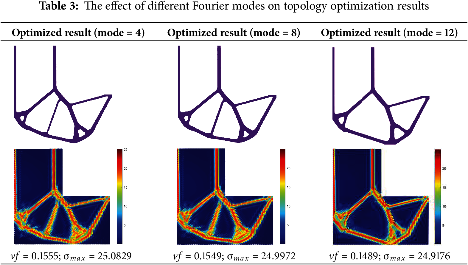
In our implementation, we chose the default value of 12 Fourier modes based on findings from our previous work [41], where we observed that using 12 modes provides a good balance between accuracy and computational cost across a range of PDE-related problems. To further investigate the sensitivity of our method to the number of Fourier modes, we conduct additional experiments based on the first case in Table 1. We compare results obtained using 4, 8, and 12 Fourier modes. The results are summarized in the following Table 3. As shown, using fewer modes (e.g., 4) slightly increases the objective value, indicating a minor degradation in performance. Increasing the number of modescan improve that.

5.2.3 Overlapping Strategy

In the methodology section, we propose an overlapping strategy to increase the training data amount available for FNO training. Next, we examine the impact of this strategy on the effectiveness of the online learning approach for stress-constrained design problems. In this study, we fix n2, while varying n1. In constructing the MG input, the overlapping ratio in both directions is set to 0.5. When n1 reduces to 5, n0 value of 21 is used. The results are summarized in Table 4. Reducing n1 decreases the number of IGA evaluations during online learning and thus reduces the computational time. But it also results in a smaller training dataset, which may negatively impact the accuracy of FNO predictions and final optimized results. It can be observed that employing the overlapping strategy can further obtain better objective function values. This demonstrates the role of overlap in generating additional datasets, which can further support the training of the FNO. This advantage becomes more pronounced when n1 is small and the amount of training data is limited, as it enables the FNO to predict sensitivities more accurately and yields volume fractions that are closer to the ground truth.

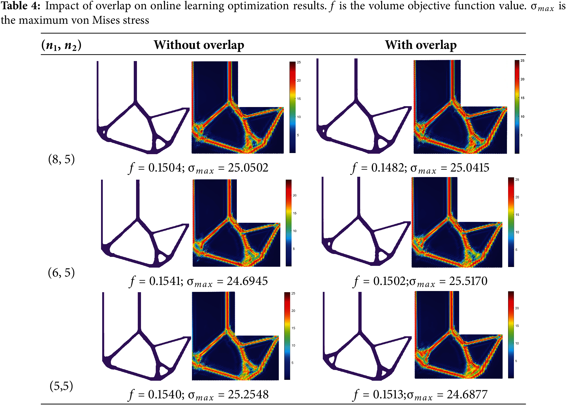
If the overlapping ratio is too small, it fails to effectively expand the dataset, whereas excessively large overlapping ratios are also not recommended. Because they will result in a higher GPU memory usage and a longer training time due to the increased number of training samples. Addition, extremely large overlapping ratios do not necessarily improve the accuracy as overfitting may occur. Therefore, a default value of 0.5 is adopted in our experiments.

5.2.4 Efficiency

As shown in Table 1, the online learning approach reduces the total amount of computational time of the two design problems. However, the reduced amount is rather small, which is less than 20%. There are two main reasons for the small improvement in efficiency. First, a relatively small n2 to n1 ratio was employed in those calculations. Since the speedup is controlled by the ratio of ground truth computation time to the online learning solution time, to further enhance the speedup achieved by the online learning method, a smaller n1 value and thus a larger ratio could be used, as demonstrated in Table 4. Reducing n1 to 5 (with overlap) shortens the total computation time to 1767.56 s, yielding a speedup of 1.44, which is larger than the speedup of 1.23 in Table 1.

Second, the size of the two problems considered is rather small (103 × 52), it is expected a larger efficiency gain would be obtained for large-scale problems. We examine two additional design cases of different design resolutions, but with the same problem setup as shown in Fig. 7a. The control point grids are set to (a) 63 × 48 and (b) 207 × 102, respectively. After padding, the input sizes of FNO are 64 × 48 and 208 × 104, respectively. For the larger case, the filter radius is 8 and n0 is 25, while other parameters remain unchanged.

The design results of the two additional cases are provided in Table 5. As shown, compared to the case with the size of 103 × 52, the speedup drops to 1.29× in case (a), while increasing to 1.78× in case (b). Based on the results from these three experiments, we plot the relationship between speedup and the number of control points, as shown in Fig. 13. As the number of control points increases, the speedup gradually approaches the theoretical upper limit value of (n1+n2)/n1. In the case when n1=n2=5, this value is 2.0.

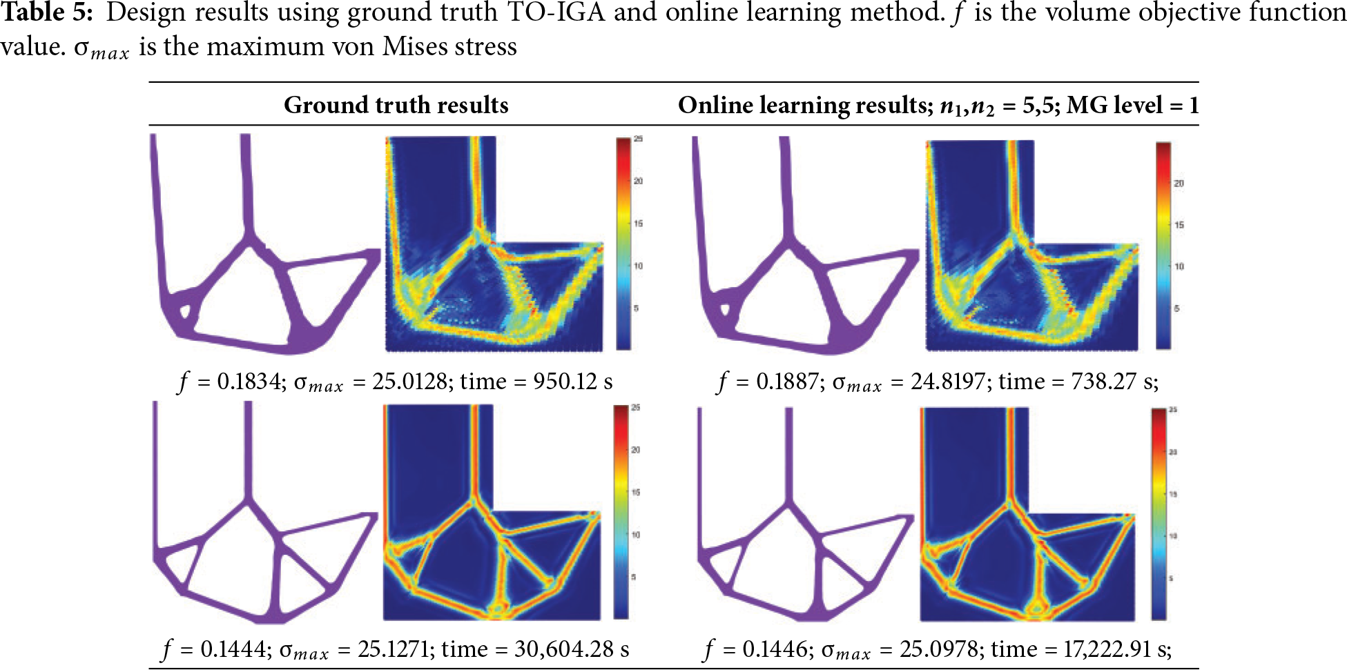
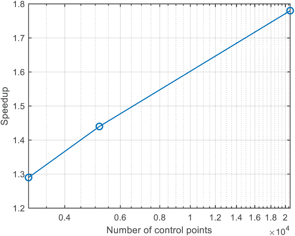
Figure 13: The relationship between speedup and the number of control points

The trade-off between efficiency and accuracy is inherent in machine learning methods and is often difficult to analyze theoretically. However, our numerical experiments (including compliance design cases) indicate that a relative error of approximately 0.1% yields satisfactory designs with performance comparable to the ground-truth solution. The training data required to achieve this error threshold depends on the problem’s complexity. The adaptive hierarchical strategy proposed in [29] can be employed to select appropriate multigrid levels and overlapping ratios based on a targeted speedup ratio.

In addition to the increased speedup achieved as the number of control points increases, the results also show that the objective function decreases from 0.1887 to 0.1446. Moreover, the optimized topology becomes more complex with refinement: the design contains four holes for the first two cases, whereas five holes appear in the finest mesh. These observations are consistent with the expectation since the design space expands as the number of control points increases.

6  Conclusion

This work presents an online learning framework to improve efficiency of isogeometric topology optimization, where the FNO surrogate is employed to predict sensitivity fields. A multi-grid decomposition strategy is employed, enabling the augmentation of training data and embedding global information across different levels in the input. This strategy enhances framework scalability and FNO prediction accuracy. The results of numerical experiments demonstrate the effectiveness of the proposed framework across two stress constrained design problems. By incorporating FNO as surrogate models, the framework significantly reduces the number of IGA evaluations and sensitivity calculations, leading to substantial computational savings while maintaining results comparable to ground-truth IGA solutions in large-scale examples. Reducing the usage ratio of IGA updates can further improve efficiency; however, this also reduces the amount of available data, which may negatively impact the accuracy of FNO predictions. Therefore, there’s a tradeoff between efficiency and accuracy. Overlapping strategy can help increase the training dataset size, which can enhance the FNO’s prediction accuracy.

There remain multiple promising directions for future research. For example, future efforts could focus on dynamically adjusting the FNO usage ratio during inference, possibly guided by design change indicators. Additionally, while the framework is validated on medium-scale problems, its scalability to giga-scale and 3D stress-constrained designs remain undemonstrated. Future work will include such large-scale 3D stress-constrained design problems and extensions to other application problems, such as acoustic wave analysis.

Acknowledgement: Not applicable.

Funding Statement: This work is supported by the Hong Kong Research Grants under Competitive Earmarked Research Grant No. 16206320.

Author Contributions: The authors confirm their contribution to the paper as follows: study conception and design: Wenjing Ye; data collection: Kangjie Li; analysis and interpretation of results: Kangjie Li, Wenjing Ye; draft manuscript preparation: Kangjie Li. All authors reviewed the results and approved the final version of the manuscript.

Availability of Data and Materials: Data available on request from the authors.

Ethics Approval: Not applicable.

Conflicts of Interest: The authors declare no conflicts of interest to report regarding the present study.

References

1. Bendsøe MP, Sigmund O. Material interpolation schemes in topology optimization. Arch Appl Mech. 1999;69:635–54. doi:10.1007/s004190050248. [Google Scholar] [CrossRef]

2. de Troya MA S, Tortorelli DA. Adaptive mesh refinement in stress-constrained topology optimization. Struct Multidiscip Optim. 2018;58(6):2369–86. doi:10.1007/s00158-018-2084-2. [Google Scholar] [CrossRef]

3. Wang S, de Sturler E, Paulino GH. Dynamic adaptive mesh refinement for topology optimization. arXiv:1008.3453. 2010. [Google Scholar]

4. Hoshina TY, Menezes IF, Pereira A. A simple adaptive mesh refinement scheme for topology optimization using polygonal meshes. J Braz Soc Mech Sci Eng. 2018;40(7):348. doi:10.1007/s40430-018-1267-5. [Google Scholar] [CrossRef]

5. Hughes TJ, Cottrell JA, Bazilevs Y. Isogeometric analysis: CAD, finite elements, NURBS, exact geometry and mesh refinement. Comput Methods Appl Mech Eng. 2005;194(39–41):4135–95. doi:10.1016/j.cma.2004.10.008. [Google Scholar] [CrossRef]

6. Cottrell JA, Hughes TJ, Bazilevs Y. Isogeometric analysis: toward integration of CAD and FEA. Chichester, UK: John Wiley & Sons; 2009. 352 p. [Google Scholar]

7. Seo YD, Kim HJ, Youn SK. Isogeometric topology optimization using trimmed spline surfaces. Comput Methods Appl Mech Eng. 2010;199(49–52):3270–96. doi:10.1016/j.cma.2010.06.033. [Google Scholar] [CrossRef]

8. Dedè L, Borden MJ, Hughes TJ. Isogeometric analysis for topology optimization with a phase field model. Arch Comput Methods Eng. 2012;19:427–65. doi:10.1007/s11831-012-9075-z. [Google Scholar] [CrossRef]

9. Chen W, Su X, Liu S. Algorithms of isogeometric analysis for MIST-based structural topology optimization in MATLAB. Struct Multidiscip Optim. 2024;67(3):43. doi:10.1007/s00158-024-03764-4. [Google Scholar] [CrossRef]

10. Wang Y, Benson DJ. Isogeometric analysis for parameterized LSM-based structural topology optimization. Comput Mech. 2016;57:19–35. doi:10.1007/s00466-015-1219-1. [Google Scholar] [CrossRef]

11. Qiu W, Wang Q, Gao L, Xia Z. Evolutionary topology optimization for continuum structures using isogeometric analysis. Struct Multidiscip Optim. 2022;65(4):121. doi:10.1007/s00158-022-03215-y. [Google Scholar] [CrossRef]

12. Hou W, Gai Y, Zhu X, Wang X, Zhao C, Xu L, et al. Explicit isogeometric topology optimization using moving morphable components. Comput Methods Appl Mech Eng. 2017;326:694–712. doi:10.1016/j.cma.2017.08.021. [Google Scholar] [CrossRef]

13. Shaaban AM, Anitescu C, Atroshchenko E, Rabczuk T. 3D isogeometric boundary element analysis and structural shape optimization for Helmholtz acoustic scattering problems. Comput Methods Appl Mech Eng. 2021;384:113950. doi:10.1016/j.cma.2021.113950. [Google Scholar] [CrossRef]

14. Shaaban AM, Anitescu C, Atroshchenko E, Rabczuk T. Isogeometric boundary element analysis and shape optimization by PSO for 3D axi-symmetric high frequency Helmholtz acoustic problems. J Sound Vib. 2020;486:115598. doi:10.1016/j.jsv.2020.115598. [Google Scholar] [CrossRef]

15. Wang J, Jiang F, Zhao W, Chen H. A combined shape and topology optimization based on isogeometric boundary element method for 3D acoustics. Comput Model Eng Sci. 2021;127(2):645–81. doi:10.32604/cmes.2021.015894. [Google Scholar] [CrossRef]

16. Hassani B, Khanzadi M, Tavakkoli SM. An isogeometrical approach to structural topology optimization by optimality criteria. Struct Multidiscip Optim. 2012;45:223–33. doi:10.1007/s00158-011-0680-5. [Google Scholar] [CrossRef]

17. Gao J, Gao L, Luo Z, Li P. Isogeometric topology optimization for continuum structures using density distribution function. Int J Numer Methods Eng. 2019;119(10):991–1017. doi:10.1002/nme.6081. [Google Scholar] [CrossRef]

18. Gao J, Wang L, Luo Z, Gao L. IgaTop: an implementation of topology optimization for structures using IGA in MATLAB. Struct Multidiscip Optim. 2021;64:1669–700. doi:10.1007/s00158-021-02858-7. [Google Scholar] [CrossRef]

19. Zhuang C, Xiong Z, Ding H. An efficient 2D/3D NURBS-based topology optimization implementation using page-wise matrix operation in MATLAB. Struct Multidiscip Optim. 2023;66(12):254. doi:10.1007/s00158-023-03701-x. [Google Scholar] [CrossRef]

20. da Silva GA, Aage N, Beck AT, Sigmund O. Local versus global stress constraint strategies in topology optimization: a comparative study. Int J Numer Methods Eng. 2021;122(21):6003–36. doi:10.1002/nme.6781. [Google Scholar] [CrossRef]

21. Kazemi HS, Tavakkoli SM, Naderi R. Isogeometric topology optimization of structures considering weight minimization and local stress constraints. Int J Optim Civ Eng. 2016;6(2):303–17. [Google Scholar]

22. Svanberg K. The method of moving asymptotes—a new method for structural optimization. Int J Numer Methods Eng. 1987;24(2):359–73. doi:10.1002/nme.1620240207. [Google Scholar] [CrossRef]

23. Jahangiry HA, Tavakkoli SM. An isogeometrical approach to structural level set topology optimization. Comput Methods Appl Mech Eng. 2017;319:240–57. doi:10.1016/j.cma.2017.02.005. [Google Scholar] [CrossRef]

24. Liu H, Yang D, Hao P, Zhu X. Isogeometric analysis based topology optimization design with global stress constraint. Comput Methods Appl Mech Eng. 2018;342:625–52. doi:10.1016/j.cma.2018.08.013. [Google Scholar] [CrossRef]

25. Zhai X. Alternating optimization method for isogeometric topology optimization with stress constraints. J Comput Math. 2024;42(1):134–55. doi:10.4208/jcm.2209-m2021-0358. [Google Scholar] [CrossRef]

26. Villalba D, Gonçalves M, Dias-de-Oliveira J, Andrade-Campos A, Valente R. IGA-based topology optimization in the design of stress-constrained compliant mechanisms. Struct Multidiscip Optim. 2023;66(12):244. doi:10.1007/s00158-023-03697-4. [Google Scholar] [CrossRef]

27. Gao J, Gao L, Xiao M. Isogeometric topology optimization: methods, applications and implementations. Singapore: Springer; 2022. 212 p. [Google Scholar]

28. Vo D, Nguyen MN, Bui TQ, Suttakul P, Rungamornrat J. Isogeometric gradient-free proportional topology optimization (IGA-PTO) for compliance problem. Int J Numer Methods Eng. 2023;124(19):4275–310. doi:10.1002/nme.7315. [Google Scholar] [CrossRef]

29. Li K, Ye W. A multi-grid, single-mesh online learning framework for efficient large-scale topology optimization. Eng Comput. Forthcoming. 2025. [Google Scholar]

30. Toan ML, Elena A, Tinh QB, Jaroon R. Material and thickness optimization of microscale in-plane FG thin-walled structures using deep neural network-assisted artificial hummingbird lgorithms. Comp Struct. 2025;368:119227. doi:10.1016/j.compstruct.2025.119227. [Google Scholar] [CrossRef]

31. Woldseth RV, Aage N, Bærentzen JA, Sigmund O. On the use of artificial neural networks in topology optimisation. Struct Multidiscip Optim. 2022;65(10):294. doi:10.1007/s00158-022-03347-1. [Google Scholar] [CrossRef]

32. Xiang C, Wang D, Pan Y, Chen A, Zhou X, Zhang Y. Accelerated topology optimization design of 3D structures based on deep learning. Struct Multidiscip Optim. 2022;65(3):99. doi:10.1007/s00158-022-03194-0. [Google Scholar] [CrossRef]

33. Gao Y, Zhou S, Li M. Structural topology optimization based on deep learning. J Comput Phys. 2025;520:113506. doi:10.1016/j.jcp.2024.113506. [Google Scholar] [CrossRef]

34. Xue L, Liu J, Wen G, Wang H. Efficient, high-resolution topology optimization method based on convolutional neural networks. Front Mech Eng. 2021;16(1):80–96. doi:10.1007/s11465-020-0614-2. [Google Scholar] [CrossRef]

35. Chi H, Zhang Y, Tang TLE, Mirabella L, Dalloro L, Song L, et al. Universal machine learning for topology optimization. Comput Methods Appl Mech Eng. 2021;375:112739. doi:10.1016/j.cma.2019.112739. [Google Scholar] [CrossRef]

36. Piegl L, Tiller W. The NURBS book. 2nd ed. Berlin, Germany: Springer; 1997. 646 p. [Google Scholar]

37. Wendland H. Piecewise polynomial, positive definite and compactly supported radial functions of minimal degree. Adv Comput Math. 1995;4:389–96. doi:10.1007/bf02123482. [Google Scholar] [CrossRef]

38. Giraldo-Londoño O, Paulino GH. PolyStress: a Matlab implementation for local stress-constrained topology optimization using the augmented Lagrangian method. Struct Multidiscip Optim. 2021;63(4):2065–97. doi:10.1007/s00158-020-02760-8. [Google Scholar] [CrossRef]

39. Holmberg E, Torstenfelt B, Klarbring A. Stress constrained topology optimization. Struct Multidiscip Optim. 2013;48:33–47. doi:10.1007/s00158-012-0880-7. [Google Scholar] [CrossRef]

40. Li Z, Kovachki N, Azizzadenesheli K, Liu B, Bhattacharya K, Stuart A, et al. Fourier neural operator for parametric partial differential equations. arXiv:2010.08895. 2020. [Google Scholar]

41. Li K, Ye W. D-FNO: a decomposed Fourier neural operator for large-scale parametric partial differential equations. Comput Methods Appl Mech Eng. 2025;436:117732. doi:10.1016/j.cma.2025.117732. [Google Scholar] [CrossRef]

42. Kossai J, Kovachki N, Azizzadenesheli K, Anandkumar A. Multi-grid tensorized Fourier neural operator for high-resolution PDEs. Trans Mach Learn Res. 2024;8:1–27. [Google Scholar]