Data-Driven Component-Level Decision-Making for Online Remanufacturing of Gas-Insulated Switchgear

1  Introduction

Remanufacturing involves the refurbishment of used products, referred to as “cores,” to a state comparable to their original, new condition [1]. This process is structured and encompasses several critical stages, including the acquisition of cores, disassembly, cleaning, inspection, repair, and reassembly. This comprehensive approach ensures that the functionality of remanufactured products is similar to that of newly manufactured ones. Therefore, remanufacturing is recognized as an efficient and promising strategy for recycling finite resources and energy, reducing pollution in the manufacturing sector, enhancing material efficiency, and contributing to environmental sustainability [2,3].

The diverse and significant benefits of remanufacturing are gaining increasing recognition and adoption in various industrial sectors. Jensen et al. [4] explored the integration of remanufacturing practices within the business models of three companies. The remanufacturing efforts of Siemens Wind Power focused on wind turbines. This approach extends the turbine service life and introduces a novel revenue stream through after-sales upgrades, demonstrating significant environmental benefits by increasing resource efficiency. Orangebox integrated remanufacturing into its business model by designing chairs that can be easily disassembled and remanufactured. This strategy opened new market segments by offering high-quality, remanufactured products at lower costs. Philips refurbished its medical devices. This practice reduces material usage by up to 80% and facilitates access to high-quality medical devices at lower costs, catering to a broader range of customers while supporting sustainability goals. Beyond these instances, a significant body of research has emphasized the environmental and economic benefits of remanufacturing [5–8]. Therefore, continuous investigations in this field are crucial to encourage sustainable production practices and unlock the comprehensive potential of remanufacturing across various sectors.

Despite the growing recognition of remanufacturing as a sustainable and cost-effective practice, its practical implementation still faces several challenges. In real industrial settings, one of the most critical tasks is determining when and what to remanufacture. These decisions must balance technical, economic, and operational factors while accounting for the inherent uncertainty in equipment degradation. To address this practical challenge, this study introduces a data-driven framework that supports both the timing and the component-level decisions in remanufacturing.

1.1 Motivation

To effectively perform remanufacturing, determining the optimal timing of the process is crucial. The first step is to assess the equipment condition and optimize the remanufacturing schedule based on this condition and other influencing factors [9–12]. However, existing studies predominantly rely on mathematical models to evaluate equipment performance. While these models offer a structured approach for estimating product functionality, their accuracy can vary depending on the operational environment, and they often struggle to capture specific product characteristics. For instance, products subjected to harsher conditions may deteriorate faster, necessitating adjustments to standard mathematical models. In the optimization stage, previous approaches commonly adopt offline optimization techniques, which assume access to the complete time series of decision factors. This assumption is impractical in real-world applications, where data are sequentially collected in an online manner, making complete information unavailable. Moreover, prior studies typically focus solely on identifying the optimal timing for remanufacturing, without providing guidance on which components should be replaced. As a result, existing decision-making approaches may not generalize well across diverse operational scenarios.

1.2 Novelty

To address the limitations of previous studies, this work introduces a data-driven approach for predicting equipment performance, enabling online optimization, and supporting component-level decision-making. Specifically, a model is trained to predict the remaining useful life (RUL) of each piece of equipment using data collected from its operational environment. The model is continuously updated through an online learning strategy that incorporates incoming data to improve the accuracy of lifespan assessment. Based on the updated model, remanufacturing simulations are performed to estimate the potential profit and associated costs. These simulations also identify which specific components should be replaced, enabling precise, component-level decisions. The estimated profit and cost are integrated into a unified decision value that quantifies the benefit of remanufacturing at each timestep. The optimal remanufacturing timing is then determined online by identifying the point at which this decision value reaches its maximum.

Compared with existing remanufacturing decision-making frameworks, the proposed approach introduces three key innovations. First, it removes the reliance on predefined mathematical degradation models by adopting a data-driven RUL prediction model. This data-driven approach improves prediction accuracy and adaptability to equipment-specific conditions. Second, it incorporates an online optimization mechanism that determines the optimal remanufacturing timing using only past and current data. This allows more realistic decision-making compared with previous offline approaches that assume access to future information. Finally, the framework extends decision-making to the component-level, providing actionable guidance on which specific parts should be replaced. These advancements collectively enhance both the accuracy and practicality of remanufacturing decisions, offering a more interpretable and effective solution for real-world industrial applications.

1.3 Structure of the Article

The remainder of this paper is structured as follows. Section 2 reviews the related work. Section 3 presents the details of the methodology, initially explaining the equipment performance prediction model and subsequently describing the proposed framework. Section 4 introduces a case study of the proposed framework, Section 5 discusses the findings, and Section 6 concludes the paper.

2  Related Work

2.1 Remanufacturing Timing Decision-Making

Decision-making science provides a theoretical foundation for selecting optimal actions under uncertainty, balancing multiple objectives such as cost, reliability, and environmental impact. In engineering applications, decision-making frameworks have evolved from traditional cost–benefit analysis to multi-criteria decision-making (MCDM) approaches. Recent studies have explored these mathematical frameworks for decision support in uncertain contexts. For example, Haque et al. [13] applied linguistic trapezoidal neutrosophic sets with Einstein operators to an e-learning app selection problem, while Banik et al. [14] developed a cylindrical neutrosophic MCDM approach to support complex purchasing decisions. However, such methods are inadequate for remanufacturing timing decisions due to the complexity and dynamic nature of modern industrial systems. Equipment conditions evolve continuously, and decision factors change over time, making it difficult to rely solely on expert judgment. Therefore, in the context of remanufacturing, research has increasingly focused on developing frameworks that minimize dependence on human judgment.

In the context of remanufacturing, various types of decision-making problems arise. For instance, Dong and Dai [15] examined alliance strategies in dual-channel remanufacturing supply chains, and Zhou et al. [16] investigated strategic planning in closed-loop supply chains. While such works provide valuable insights into high-level strategic planning for remanufacturing systems, our study differs by focusing on operational decision-making. One key operational consideration in remanufacturing is the management and utilization of end-of-life (EOL) products. Consequently, many studies have examined remanufacturing decisions based on EOL core conditions. Yi et al. [17] concentrate on designing a closed-loop supply chain network and examining the process from a retailer’s viewpoint. Yang et al. [18] develop a comprehensive decision support tool based on an analysis of product- and part-level remanufacturing feasibility. Liao et al. [19] introduced a methodology for evaluating environmental efficiency and refining the production strategy for remanufacturing EOL machines. Moon et al. [20] established a model for forecasting the remaining lifespan of equipment and proposed a framework for automatically identifying the components of an EOL product that should be replaced to optimize remanufacturing outcomes. These studies generally assume that the core, serving as the raw material for remanufacturing, has already reached its EOL state. However, the EOL state does not necessarily represent the most advantageous timing for initiating the remanufacturing process. As a result, recent research has increasingly focused on determining the optimal timing for remanufacturing.

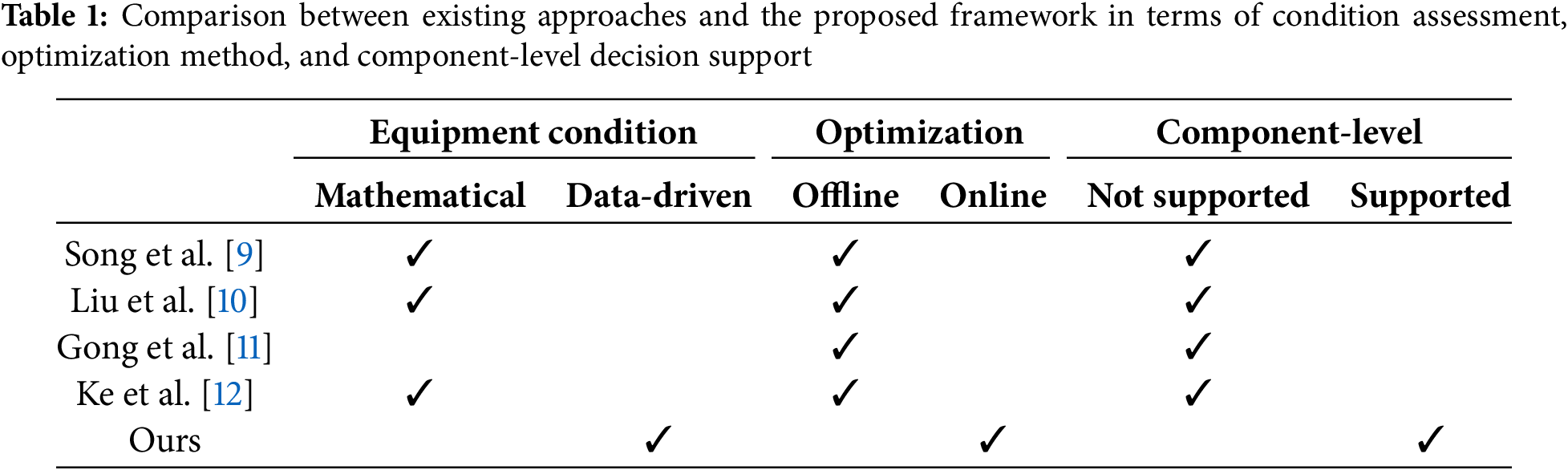
Song et al. [9] proposed a proactive approach for determining remanufacturing timing by calculating component residual strength, remanufacturing value, and technical feasibility. Liu et al. [10] introduced an optimal timing model for remanufacturing, combining replacement theory and environmental factors. Gong et al. [11] proposed a multi-objective optimization model, executed via particle swarm optimization, to aid strategic remanufacturing decisions that align economic and environmental objectives. Ke et al. [12] introduced the decision-making process for remanufacturing timing, focusing on evaluating product performance based on the structural failures of key components through online monitoring. However, these approaches generally rely on predefined mathematical models, require offline optimization, and do not support component-level decision-making, which may limit their applicability to real-world decision-making scenarios.

Table 1 highlights the differences between the proposed methodology and prior approaches. In previous studies, assessing equipment conditions relied on mathematical modeling. However, the proposed method evaluates equipment conditions based on online data collected during operation, enabling an accurate assessment of the equipment’s state. Moreover, when optimizing remanufacturing timing based on quantified metrics, prior research often assumes access to complete information across all timesteps, thus relying on offline optimization. However, the proposed approach uses only the information available up to the current timestep and performs optimization in an online setting. This online capability supports more practical and adaptable decision-making in real-world applications. In addition, previous works have primarily focused on determining when remanufacturing should occur, without addressing what components should be repaired. In contrast, the proposed framework enables component-level decision-making, allowing for the identification of specific parts that should be repaired to optimize the overall remanufacturing process.

2.2 Remaining Useful Lifetime Prediction

Evaluating product performance is crucial for making timely remanufacturing decisions. To achieve this, the RUL, a key metric for assessing equipment performance, was used as an indicator of the current equipment state [21–23]. Traditional RUL prediction methods predominantly rely on statistical and physics-based approaches. Li et al. [24] demonstrated the use of stochastic prognostics for rolling element bearings, highlighting the ability of probabilistic models to capture wear progression over time. Banjevic and Jardine [25] applied hidden Markov models to track the health state of machinery components, enabling the estimation of RUL based on observed data sequences. However, traditional RUL prediction models generally assume specific operating conditions, such as linear degradation patterns. These assumptions limit their adaptability to diverse and dynamic operational settings. As a result, these models often struggle to provide reliable predictions in complex or evolving environments, underscoring the need for more flexible and robust approaches.

Machine learning techniques have significantly advanced the field of RUL prediction, offering enhanced adaptability and accuracy over traditional methods. da Costa et al. [21] improved RUL prediction under varying operating conditions by applying domain adaptation to address distribution shift. Chen et al. [22] enhanced RUL prediction accuracy by combining handcrafted and learned features with an attention mechanism that emphasizes important features and timesteps. Yan et al. [23] achieved accurate RUL prediction by using a long short-term memory (LSTM) model to estimate a health indicator that captures the transition from a healthy to a degraded state. Wang et al. [26] improved bearing RUL prediction by combining feature selection using the RReliefF algorithm with an extreme learning machine, demonstrating that integrating relevant feature weighting can enhance prediction performance. In studies using machine learning techniques for RUL prediction, it is commonly assumed that the entire dataset is available beforehand. However, for online decision-making, RUL prediction must be conducted based on data collected online. This need has led to a growing body of research focusing on online RUL prediction.

Peng et al. [27] proposed a multivariate degradation model combined with a batch particle filter, enabling online estimation of degradation states and improving the accuracy of individualized RUL predictions. Similarly, Wang et al. [28] developed an online RUL prediction framework for lithium-ion batteries by integrating LSTM networks with an attention mechanism to capture complex degradation patterns effectively. Zhuang et al. [29] addressed data scarcity in RUL prediction by applying multi-source adversarial adaptation and online learning, allowing the model to generalize well under unseen operating conditions. These studies primarily focus on developing online prediction models that can process online data to estimate RUL. However, our research extends beyond prediction by proposing a comprehensive framework that integrates these online models to support online decision-making. This framework not only predicts RUL but also provides immediate and actionable insights, enabling enhanced operational efficiency and reliability in dynamic environments.

3  Proposed Framework

Fig. 1 summarizes the workflow of the proposed framework. At each timestep t, incoming data are divided into a training set, used to update the RUL prediction model via the online-learning technique (Section 3.1), and a test set, used in the remanufacturing simulation (Section 3.2). The updated model drives the simulation to estimate the expected profit and cost of remanufacturing (Sections 3.2 and 3.3). Finally, these estimates are combined into a decision value that guides the remanufacturing decision-making process, as detailed in Section 3.4. The symbols used throughout this framework are summarized in Table 2.

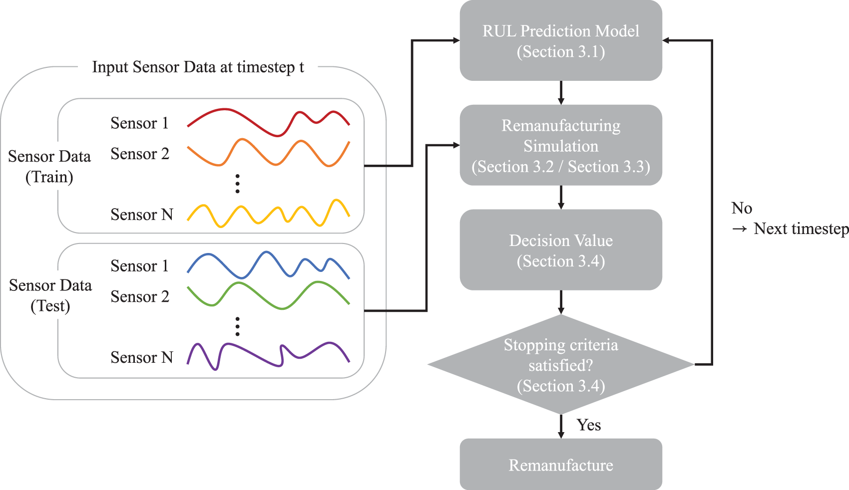
Figure 1: The overall process of the proposed framework

3.1 Remaining Useful Life Prediction with Online Data

The continual inflow of streaming sensor data rapidly expands the dataset, driving up both storage demands and model-training time. To mitigate this issue, we use an online machine learning technique: each incoming batch is used once to update the model, after which the raw data are discarded. This strategy enables continuous improvement without incurring additional storage overhead or prolonged training time.

In conventional machine learning, the task is to identify a function f that maps inputs x to targets y:

y=f(x)(1)

Training is performed on a fixed dataset, and the resulting model remains static unless an explicit retraining phase is launched. Online machine learning addresses environments where data arrive sequentially. At timestep t, the system observes an input–output pair (xt,yt) and immediately refines the current model ft−1, yielding an updated model ft:

yt=ft(xt)(2)

Because ft is initialized from ft−1, the model retains prior knowledge while adapting to the newest observations, an essential property for online decision-making systems.

To support efficient RUL prediction in an online setting, we adopt linear models that can be updated incrementally. Since the model must be updated frequently in the online environment, linear models are chosen for their low training cost and computational efficiency. Specifically, we use Linear Regression (LR) and Passive-Aggressive (PA) algorithms, both of which allow rapid online parameter updates. Both models enable efficient updates as new data arrive, without requiring retraining from scratch. The models predict the RUL of the current timestep based on a linear combination of input data xt as follows:

y^t=wt⋅xt(3)

where wt is the model parameter that should be trained.

Conventional LR employs an ordinary least squares (OLS) algorithm for model training. However, OLS is not suitable for online model training because it requires an entire dataset for model training. To address these limitations, this study adopted stochastic gradient descent (SGD) owing to its ability to efficiently update models in real time. The incremental update mechanism of SGD, which processes data points individually or in small batches, aligns well with the dynamic nature of online data processing and model updating. The SGD update parameter based on the loss function gradient is as follows:

wt+1=wt−α∂L(wt)∂wtwhereL(wt)=12(yt−y^t)2(4)

The PA algorithm was originally developed for online learning [30]. The algorithm adopts a “passive” approach when predictions align with the actual data, resulting in minimal or no updates to the model. By contrast, when the predictions are inaccurate, the algorithm switches to an “aggressive” strategy, significantly adjusting the model weights to rectify the error. This aggressive update mechanism is specifically designed to enhance the accuracy of the model for similar future instances. The model parameters are updated according to the following mathematical formulation:

wt+1=argminw12‖w−wt‖2s.t.L(w)=0,whereL(w)=max(0,|yt−y^t|−ε)(5)

When the prediction error remains within the specified margin ε, the algorithm does not update the model parameters. Conversely, when the error exceeds this margin, an aggressive update is initiated to ensure compliance with the constraints. The closed-form solution for this update process is given as

wt+1=wt+sign⁡(yt−y^t)τtxtwhereτt=L(wt)/‖xt‖2(6)

This closed-form solution enables the PA to efficiently update the model parameters, ensuring the adaptability and accuracy of the model in online learning scenarios.

3.2 Profit of Remanufacturing

Once the RUL prediction model achieves sufficient accuracy, the potential benefits of remanufacturing can be quantified through simulation. Adapting the approach of Moon et al. [20], remanufacturing simulations involve altering specific current sensor values to their initial states. This step produces virtual operational data that would be observed if the corresponding components are refurbished. The trained RUL model is then applied to both the original and simulated datasets; the resulting difference in predicted RUL represents the expected benefit of the remanufacturing.

Fig. 2 summarizes the simulation procedure at timestep t. First, the current sensor data are fed into the RUL prediction model to obtain the baseline remaining useful life, RULt. For each of the N sensors, we generate a synthetic dataset in which the entire sequence of sensor n is replaced with its initial value, effectively simulating remanufacturing of the corresponding component. Passing these modified data through the prediction model produces RULremn, the RUL after refurbishing the components related to sensor n. Selecting the k largest values of RULremn identifies the set of repairs that provides the greatest life extension. The overall remanufacturing simulation is formalized as follows:

RULsim={RULrem1,RULrem2,…,RULremN}(7)

RULtopk=TopK⁡(RULsim,k)(8)

RULrem=∑RULn,RULn∈RULtopk(9)

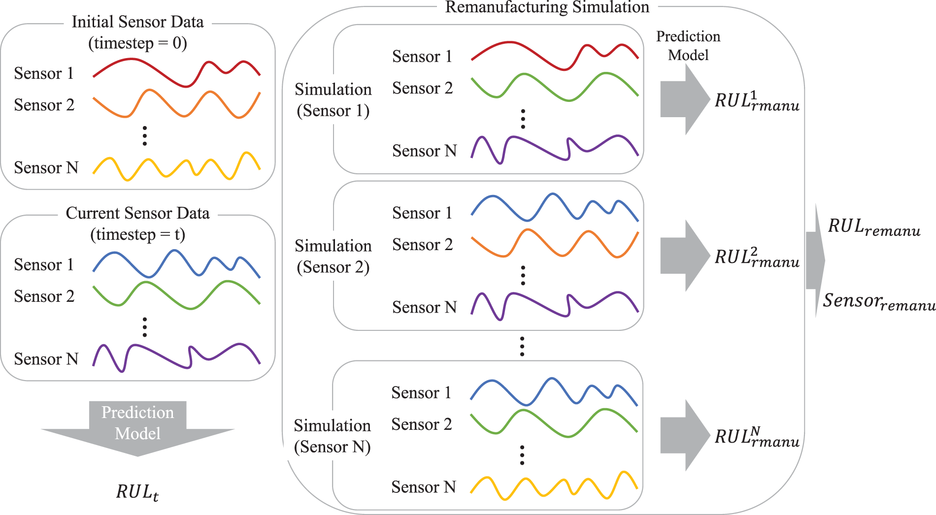
Figure 2: Remanufacturing simulation at timestep t. The RULrem represents the improved remaining useful life after remanufacturing. Additionally, analysis of the Sensorrem list identifies the specific sensors requiring remanufacturing based on remanufacturing simulation

where TopK⁡(S,k) returns the set of top k values over set S. The indices of RULtopk indicate the sensors whose associated components should be prioritized for remanufacturing:

Sensorrem=ArgTopK⁡(RULsim,k),(10)

with ArgTopK⁡(S,k) denoting the indices of the k largest elements in S. Notably, this component-level decision-making capability is a unique strength of the proposed method, not supported by previous approaches. The profit obtained by performing these remanufacturing actions at timestep t is then quantified as

profit=RULrem−RULt.(11)

3.3 Cost of Remanufacturing

In remanufacturing, the economic consequences of equipment degradation can be assessed with a quality-based cost model [31]. This model can be systematically implemented by adopting the Taguchi quality-loss concept [32]. According to Taguchi’s quadratic loss function, the cost increases with the square of the deviation from the target performance. Taking the RUL as the quality characteristic, the remanufacturing loss is defined as

costrem=costsen⋅(RULtar−RULtRULmax)2(12)

where RULtar is the target RUL, set to 100, RULmax represents the maximum RUL value, fixed at 100 in this study. costsen denotes the replacement cost of the sensor-related components within the equipment. In the context of a remanufacturing simulation, costsen can be calculated by summing the costs associated with all sensors in the Sensorrem list.

Malfunction cost is ultimately driven by the probability of equipment failure. When a reliable RUL prediction model is available, this probability can be updated online by comparing the current RUL with the maximum RUL. If the RUL estimate is unreliable in the early stage, we approximate failure behaviour with the bathtub curve, which divides a product’s lifetime into infant mortality, normal life, and wear-out phases. Because the RUL prediction model is least accurate in the early stages, our formulation considers only the infant mortality and normal life phases. During the infant mortality period, the failure probability decays exponentially from an initial rate, whereas in the normal life phase, it is assumed to be constant. Summing these two terms yields the probability of early failure. After a predefined time step, the failure rate is instead taken directly from the RUL predicted by the model. The malfunction cost is thus defined as:

costmal={failinit⋅exp⁡(−failinit⋅t)+failconstif t<M/2,RULmax−RULtRULmaxif t≥M/2(13)

where failinit is the initial failure rate, and failconst is a constant failure rate, as defined in the bathtub curve. M refers to the total number of operations performed by the equipment. The integration of the bathtub curve with advanced RUL prediction models ensures a more robust and comprehensive analysis of malfunction costs. Notably, the malfunction cost depends only on the current time step RUL value, RULt, and does not change based on the value of k, representing the number of sensors replaced in the remanufacturing simulation.

3.4 Decision-Making for Remanufacturing Timing

Previous studies define critical factors for determining optimal remanufacturing timing and integrating them into a single value for optimization [9–12]. These studies provide structured frameworks that convert complex, multidimensional considerations into quantifiable indicators. Building on this foundation, our framework captures the multidimensional aspects of remanufacturing by combining three key components—profit, remanufacturing cost, and malfunction cost—into a unified metric, termed the decision value. This metric drives the decision-making process and is defined as follows:

DV=λprofit⋅profit−λremanu⋅costremanu−λmal⋅costmal(14)

The decision value (DV) is defined as profit minus cost; maximizing DV, therefore, indicates the most significant net benefit from remanufacturing. Introducing a weight λi for each component lets practitioners tailor the metric to specific objectives. In practice, however, computing DV online—and pinpointing its peak—is non-trivial: future DV values are unknown, so deciding exactly when profitability is maximized remains a challenging problem.

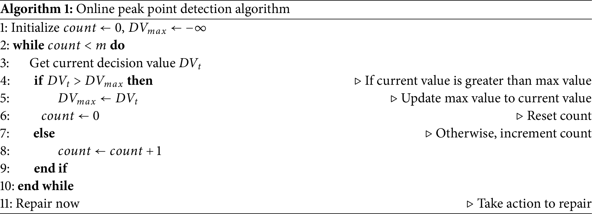
To overcome this challenge, we introduce an online peak-point detection algorithm that continuously monitors the decision value stream. At each time step, the current decision value is compared with the running maximum. If it exceeds the maximum, the maximum is updated, and a non-improvement counter is reset. If it does not, the counter is incremented. When this counter exceeds a user-defined threshold m, the system stops operation and begins remanufacturing. The full procedure is detailed in Algorithm 1.

4  Case Study

This study utilizes the dataset previously introduced in the authors’ earlier work [20], which was originally collected to develop RUL prediction models for GIS. These models supported the selection of components for repair. However, the prior study focused solely on decision-making at the equipment’s EOL stage, which may not represent the most effective timing for remanufacturing. In contrast, the present study emphasizes online decision-making for remanufacturing, better aligning with actual operational conditions. To ensure clarity and completeness, the data acquisition and preprocessing methods described in previous research are summarized in Sections 4.1 and 4.2. Figs. 3 to 6 and Table 3 are adapted from Moon et al. [20].

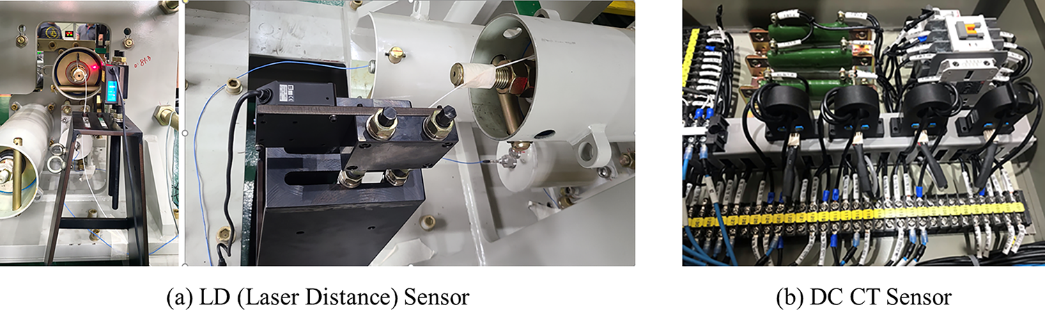
Figure 3: (a) Shows LD sensor for measuring the stroke distance. (b) shows a DC CT sensor for measuring the current of the open/close trip coil and auxiliary coil

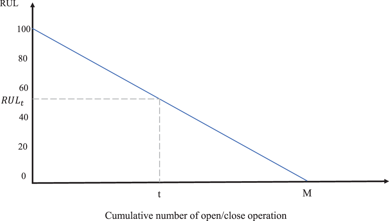
Figure 4: RUL linear function of GIS equipment

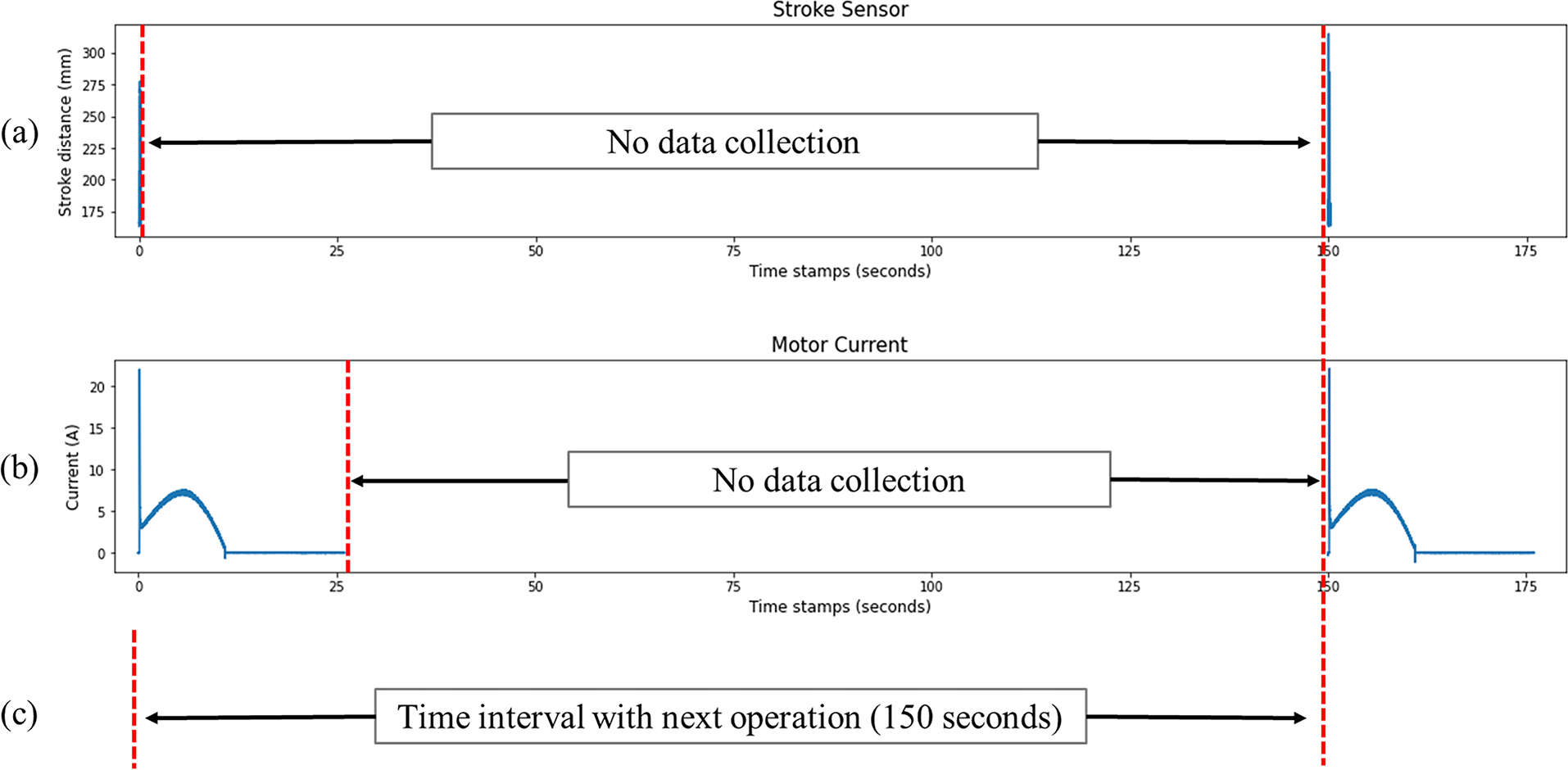
Figure 5: (a) Presents signal data sampled at 10,000 Hz, illustrating a duration of 0.28 s for each operation, with the stroke sensor specifically showcased for illustrative purposes. Apart from the motor current sensor, which operates at a different frequency, all sensors exhibit uniform frequency and operational duration. (b) shows sampled signal data from the motor current sensor, operating at a 1000 Hz frequency and capturing 26 s per operation. (c) visualizes the time intervals between operations

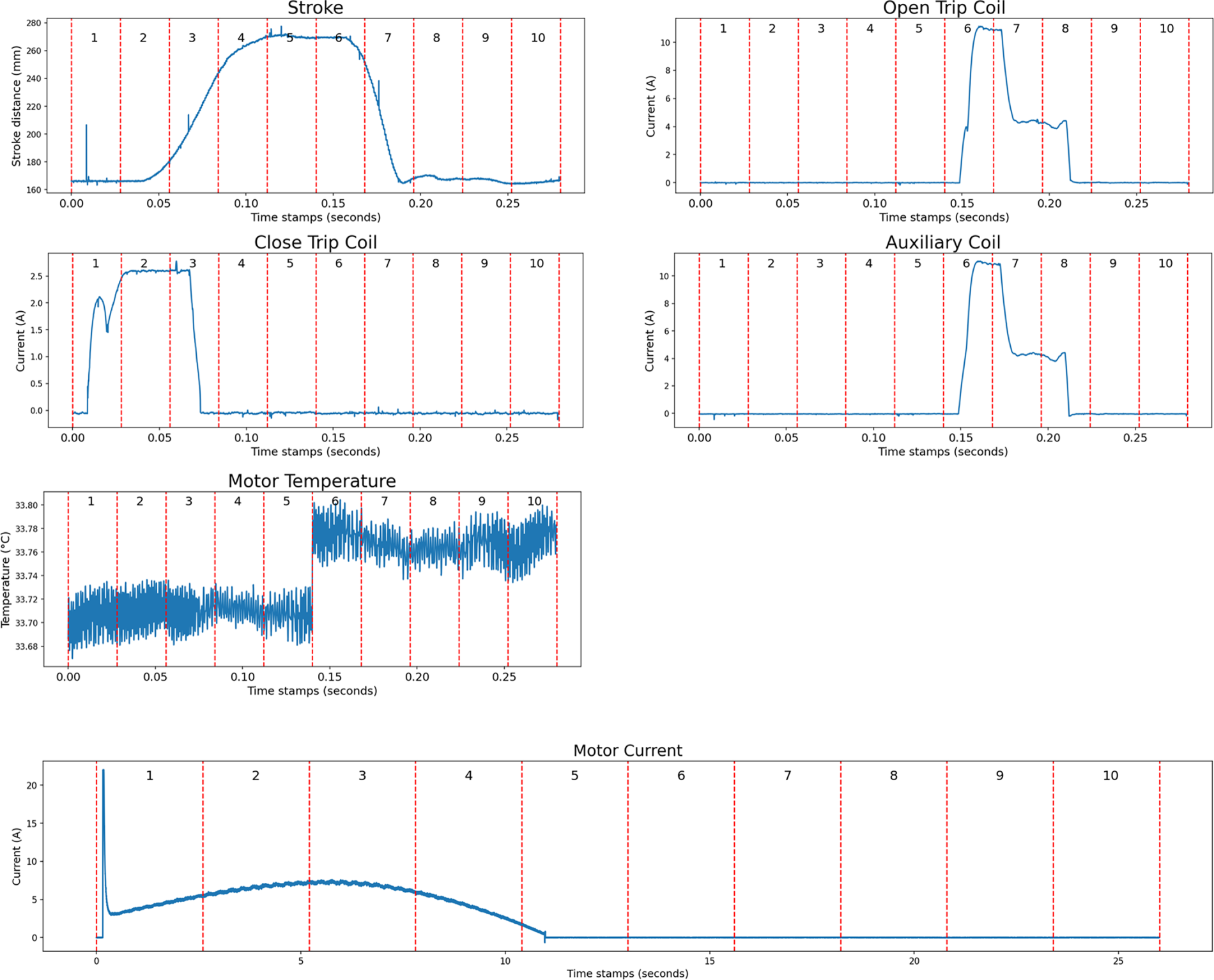
Figure 6: Segmentation of sensor signals into ten parts to analyze statistics for each open/close operation

4.1 Data Acquisition

GIS comprises several key components, including insulators, manipulators, actuators, frames, and circuit breakers. Circuit breakers play a crucial role because they interrupt the flow in a circuit and protect other electrical equipment during short-circuit incidents. Circuit breakers are categorized based on their operational mechanisms: pneumatic, hydraulic, and spring-based. The circuit interruption process involves three stages: the transformation of electrical signals into mechanical signals; the generation of an operational force via actuating valves (in pneumatic or hydraulic systems) or springs; and the application of this force to operate the circuit breaker and its connecting linkages. This study mainly focused on GIS equipped with a spring-mechanism circuit breaker, a common feature of older GIS systems. This type of equipment typically includes components, such as a hook, motor, open/close shaft, springs, and a limit switch, each playing a role in one of the three stages of the circuit-breaking process.

To gather operational data from the GIS, accelerated life testing (ALT) was performed on the GIS. ALT is essential for obtaining operational data from GIS, particularly given the typical 30- to 50-year lifespan of GIS. Recognized as an effective method for shortening data collection time, ALT is a well-known method for reducing data acquisition time by exposing equipment to an extreme environment [33,34]. In this study, the number of operational cycles was increased to stress the GIS during ALT. This test lasted for five months and continued until the GIS failed. A specific GIS model (170 kV, 50 kA, 60 Hz) with a spring-mechanism circuit breaker was used. Failure modes and effects analysis, the most widely used method for minimizing failure risks in equipment design [35], was implemented to determine the optimal sensor placement. Due to resource and time constraints, this study primarily focused on collecting sensor data from the circuit breaker, the most vital component in GIS degradation.

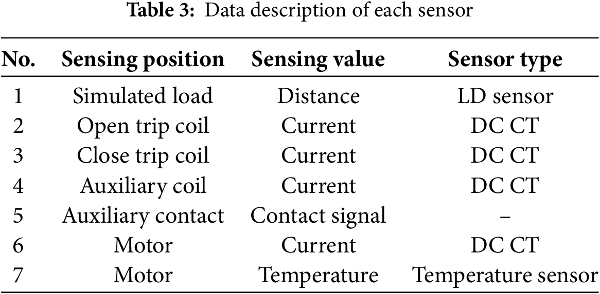
Table 3 outlines the sensors used and details their locations, measured variables, and types. The setup included seven different sensor locations and three distinct types of sensing devices. As illustrated in Fig. 3a, a laser distance (LD) sensor was used to acquire stroke information. LD sensors offer high durability and reduced vibration impact from operational cycles, ensuring superior measurement accuracy and stability compared with contact-type sensors [36]. The LD sensor was positioned on an open-spring compression plate to capture linear reciprocating motions. Fig. 3b shows the use of direct current transformer (DC CT) sensors to measure the currents from the open/close trip and auxiliary coils. DC CT sensors, designed for direct current measurements, are crucial for evaluating trip speed and damping levels after contact-point separation. Furthermore, the mechanical auxiliary contacts provided open/closed-state signals, digitized for enhanced analysis. DC CT sensors facilitated motor current monitoring, enabling the assessment of the motor state. Motor temperature sensors further enabled the evaluation of potential motor overheating.

4.2 Data Preprocessing

Training the online RUL prediction model requires the appropriate processing of GIS operational data. The data preprocessing of this study involves three primary steps: (1) defining the input and output variables and individual observations; (2) dividing the dataset into training and test subsets; and (3) normalizing the data.

In the proposed approach, the auxiliary contact signals are intentionally excluded. This exclusion is based on the understanding that the primary purpose of the auxiliary contact signal is to validate the efficacy of the open/close operation, an assessment that other signals can also provide. RUL is selected as the output variable. The RUL is conventionally calculated based on the number of operational cycles until a machine fails [20,37,38]. For instance, determining the RUL of a lithium-ion battery involves counting the charge–discharge cycles that it endures before failure [37]. In the GIS context, the RUL is calculated based on the number of open/close cycles before system failure. The upper limit of these cycles is defined as M. A linear relationship is assumed between the RUL and the cumulative number of open/close operations, as illustrated in Fig. 4. Therefore, the RUL of GIS is assumed to diminish proportionally with the number of operations. This linear degradation model is confirmed by experts in the GIS manufacturing field. Therefore, in this study, RUL is defined as follows:

RULt=(1−tM)×100, for t=1,2,3,…,M(15)

where t is the cumulative number of open/close operations.

The dataset comprises 14,359 observations, representing the maximum number of operational cycles. For each observation, all signals, excluding the motor current, were sampled at 10,000 Hz over a duration of 0.28 s. The motor current signal, however, is recorded at a lower frequency of 1000 Hz for a longer duration of 26 s. An interval of 150 s is maintained between each observation, as depicted in Fig. 5. This interval is crucial for ensuring stability during the ALT, admitting at the cost of time efficiency. To address the varying signal durations, the data from each sensor observation is segmented into ten equal parts. From each segment, seven statistical measures were extracted: mean, standard deviation, minimum, first quartile, median (second quartile), third quartile, and maximum. Fig. 6 illustrates this segmentation process for each sensor. Consequently, 70 statistical features were derived from these ten segments per sensor, resulting in a total of 420 statistical features for each observation.

To enhance the quality of the input sensor data, we applied moving-average smoothing, a common technique for noise reduction in time-series data [39]. We set the window length to 13, recalculating each data point’s value as the average of its preceding 13 data points. Subsequently, we divided the dataset into training and test subsets, using 80% for training and 20% for testing to evaluate the RUL prediction model. The input data then underwent normalization via standard scaling, a technique that adjusts data to have a mean of zero and a standard deviation of one. This standardization ensures the input data is centered around the mean with a unit standard deviation, thereby facilitating more efficient model training and evaluation.

4.3 RUL Prediction Model Selection

In an ideal scenario, the most effective way to improve model accuracy is to update the model with each newly arriving observation. However, such frequent updates impose a substantial computational burden, making this approach impractical. Therefore, this study implemented model updates using small batches of data. This strategy provides a balanced approach that maintains timely updates without incurring prohibitive computational overhead. To simulate the flow of online data and enable batch-wise updates, the dataset was partitioned into 100 segments. Each batch was processed collectively, and the arrival of a new batch triggered an update of the model. This method ensured efficient model training while satisfying the demands of online data processing.

Despite online model updating, where the model is updated with new data arrivals and the data is subsequently discarded, the model must still accurately predict the RUL for previous batches. To assess this capability, the testing protocol involved evaluating the model against the test set of the current timestep and against those of previous timesteps. This comprehensive test ensured a thorough validation of the model’s performance over time. The LR and PA algorithms were compared as RUL prediction models. However, a single linear model often struggles to capture the patterns of complex systems. To enhance robustness and predictive accuracy, an ensemble modeling technique was employed. This involved training 10 separate linear models (LR or PA) and averaging their predictions. This ensemble model leverages the combined strengths of multiple models to enhance prediction accuracy.

To further validate the proposed RUL prediction model, it was benchmarked against an “oracle model” trained on the entire dataset, including all batches from previous timesteps. Although this oracle model violates the assumptions of online learning, due to its use of complete historical data, it serves as an upper bound of performance. The comparison is conceptually straightforward: if the online learning-based model performs comparably to the oracle model, it demonstrates the proposed method’s reliability and effectiveness. For this purpose, the random forest (RF) [40], a widely used algorithm for tabular data, was employed as the oracle model.

Fig. 7a shows the R2 values across various timesteps. The oracle model, indicated by the blue line, consistently demonstrates stable and high R2 values for each timestep. Its consistently high performance facilitated benchmarking for evaluating the proposed RUL prediction model. The LR-based model (indicated by orange and red lines) showed a diminished performance at later timesteps due to its inability to adapt to evolving data patterns. In contrast, the PA-based model (represented by green and purple lines) exhibited performance closer to that of the oracle model. The PA algorithm’s strategy of prioritizing data points with larger prediction errors during training contributed to its robust performance, even under online learning settings. Initially, the single PA and ensemble PA models exhibited fluctuating prediction performances, which was attributed to the limited updates and training on a small dataset. As more timesteps were added, these models stabilized and exhibited consistent performance. Notably, the single PA model occasionally outperformed the ensemble PA model in terms of R2 value at specific timesteps. Nonetheless, the ensemble PA model generally demonstrated a more stable performance than its single counterpart. Therefore, the ensemble PA model was selected as the preferred RUL prediction model.

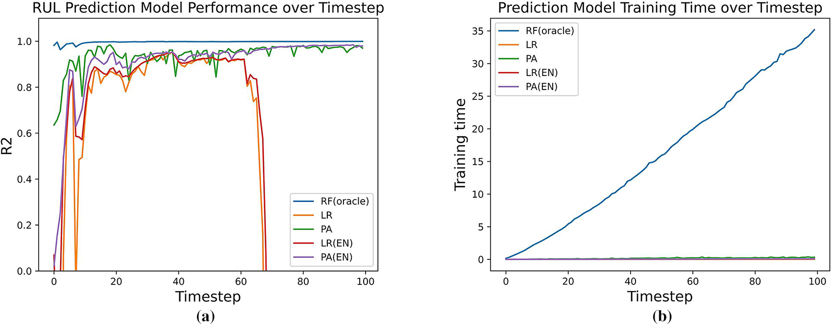
Figure 7: (a) Displays the R2 values across various timesteps. The ensemble model of the PA algorithm achieves R2 values closely aligned with those of the RF model. (b) shows the progression of training time across timesteps. The training time for the oracle model increases linearly as more timesteps are added. In contrast, other models that are updated online do not exhibit a corresponding increase in training time

Fig. 7b shows the training time across various timesteps. The training time of the oracle model increases linearly with each timestep because it uses all previous training data, highlighting the importance of introducing online machine learning algorithms. Unlike traditional machine learning algorithms, which suffer from significant scalability challenges with data volume expansion, online machine learning algorithms efficiently handle growing data without proportional increases in training time.

Table 4 presents the average R2 and mean absolute percentage error (MAPE) values across all timesteps. The 100 timesteps are divided into ten intervals, and each value represents the mean performance over ten independent runs. The best-performing model in each interval is highlighted in bold. Asterisks (*) indicate statistically significant differences between LR- and PA-based models (e.g., LR vs. PA, LR(EN) vs. PA(EN)) according to paired t-tests. Dagger symbols (†) denote statistical comparisons between the PA and ensemble PA models. The number of symbols indicates the level of statistical significance: one symbol for p< 0.1, two for p< 0.05, and three for p< 0.01.

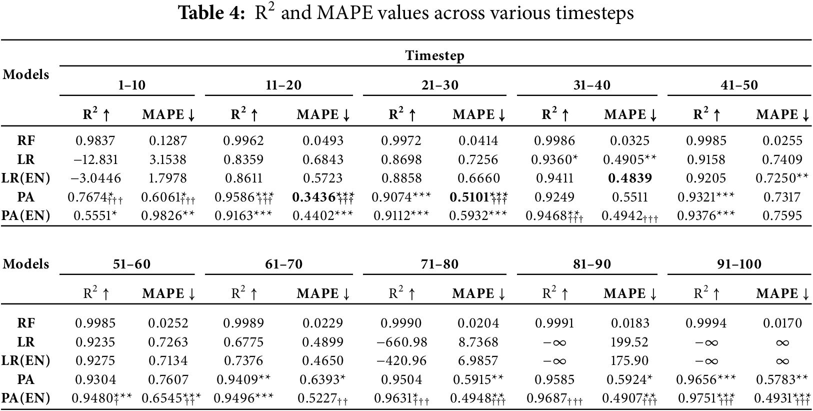
When comparing LR- and PA-based models, most intervals show asterisks on the PA variants, indicating that PA consistently outperforms LR with statistically significant improvements. This result aligns with the trend observed in Fig. 7a, where the PA algorithm’s strategy of prioritizing data points with larger prediction errors enhances robustness in online learning. In the comparison between the PA and ensemble PA models, statistical significance is not observed across all intervals. However, excluding the earliest timesteps, the ensemble PA model generally achieves higher accuracy and stability than the single PA model. Consistent with Fig. 7a, the ensemble PA model is therefore adopted as the final RUL prediction model due to its stable and reliable performance under online conditions.

4.4 Online Remanufacturing Timing Decision-Making

To determine the optimal timing for remanufacturing, this study employs a decision value, as defined in Section 3.4. This value integrates three key components—profit, remanufacturing cost, and malfunction cost—based on predictions generated by the RUL prediction model. For the computation, the weighting parameters λprofit, λremanu, and λmal were all set to 100 to balance the contribution of each factor.

The ensemble PA model, selected as the RUL predictor (Section 4.3), was used to compute the decision value according to Algorithm 1. However, the accuracy of profit and cost estimates depends on the RUL predictions, introducing a considerable amount of uncertainty. To mitigate this, a Kalman filter [41] was applied to dynamically adjust profit and cost estimates in real time, thereby enhancing the robustness of the decision-making process.

Fig. 8 presents the computed values across timesteps: (a) profit, (b) remanufacturing cost, (c) malfunction cost, and (d) the resulting decision value. These values serve as inputs to the decision algorithm, which identifies the most advantageous point for initiating remanufacturing. Based on the decision value shown in Fig. 8d, the remanufacturing process was optimally triggered at the 53rd timestep by replacing components associated with sensor index 2, with the parameters k (number of sensors to replace) and m (threshold for decision stability) set to 1 and 5, respectively.

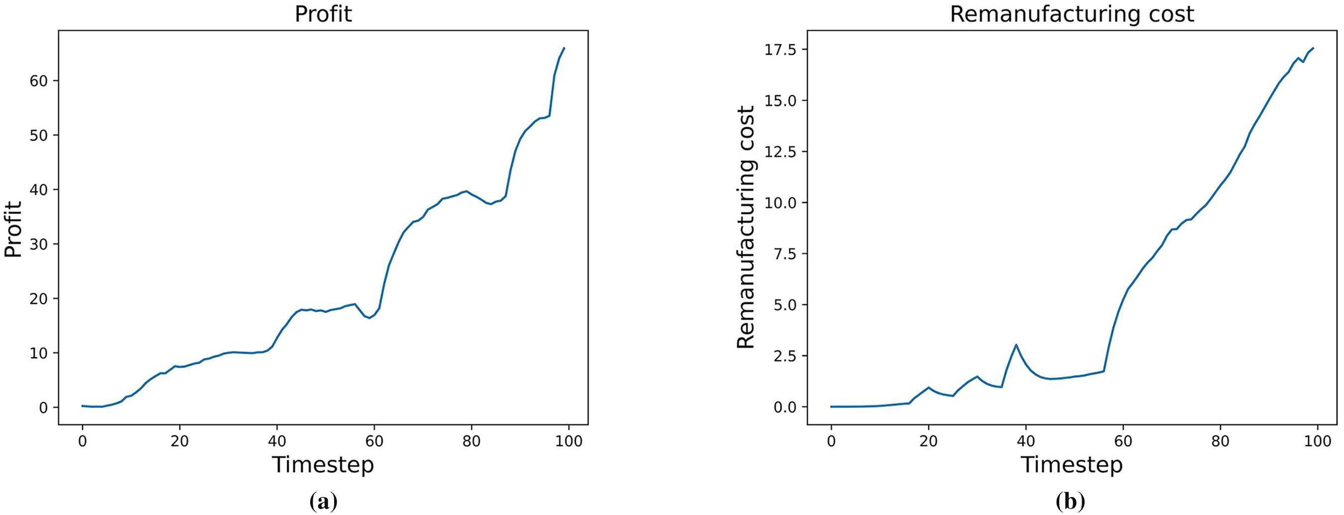
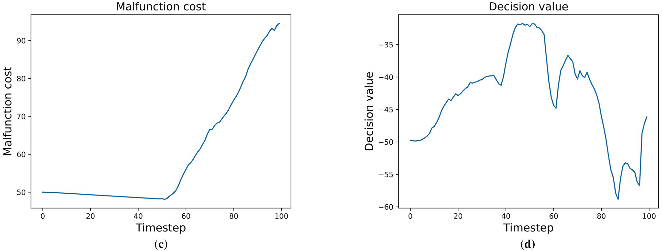
Figure 8: Calculation result of decision value and components over timestep. (a) Profit, (b) remanufacturing cost, (c) malfunction cost, and (d) decision value

To further demonstrate the effectiveness of the proposed method, we compare its remanufacturing decisions with those derived from existing approaches. Specifically, we consider the methods proposed by Song et al. [9], Ke et al. [12], and Gong et al. [11]. Song et al. determined the remanufacturing timing by considering remanufacturing value, residual strength, and feasibility. In our comparison, we mapped remanufacturing value to the predicted RUL and residual strength to the results of the remanufacturing simulation. We assumed that remanufacturing is feasible at all timesteps. Ke et al. defined the decision value as the summation of all components related to decision-making and used an offline optimization algorithm to identify the optimal timing. Gong et al. defined the decision value as the product of all related components and applied particle swarm optimization to maximize this value. It is important to note that all comparison methods rely on offline optimization, which assumes access to the entire sequence of decision values across all timesteps. This approach is not compatible with online decision-making, where only past data is available. Nevertheless, we include these methods as baselines to highlight the performance of our proposed online approach.

Fig. 9 compares the remanufacturing timing decisions obtained by each method based on the computed decision value. The solid blue line represents the evolution of the decision value over time, while the vertical dashed lines indicate the remanufacturing points selected by the compared methods. As shown, the methods proposed by Song et al. and Gong et al. trigger remanufacturing at suboptimal timesteps where the decision value is considerably lower than the global maximum, leading to inefficient use of equipment lifetime. Although Ke et al.’s offline optimization approach identifies a timing close to the peak decision value, it relies on future information that is unavailable in practice. In contrast, the proposed method determines the remanufacturing timing using only current and past data, while still achieving a decision value that is very close to the global optimum. This result demonstrates that the proposed online framework can effectively approximate the globally optimal decision without access to future information, validating both its practical feasibility and decision-making robustness under real-world operating conditions.

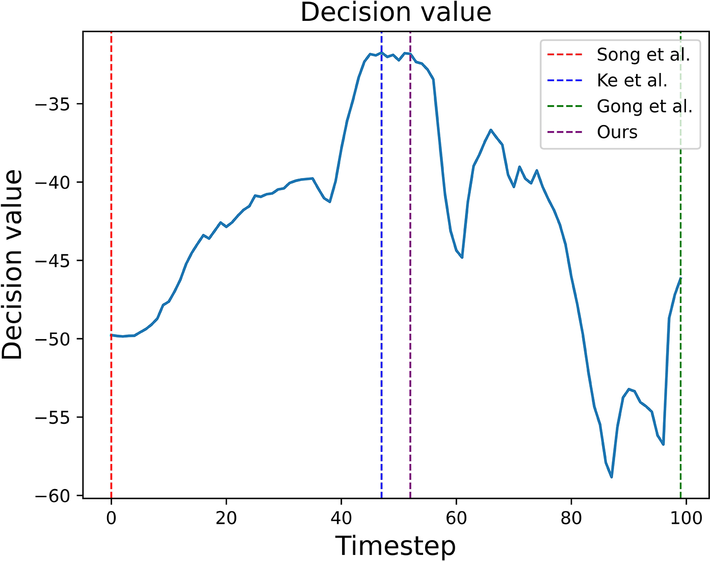
Figure 9: Comparison of remanufacturing timing based on decision value. The solid blue line represents the computed decision value over time. The vertical dashed lines indicate the remanufacturing timing determined by existing studies and our method

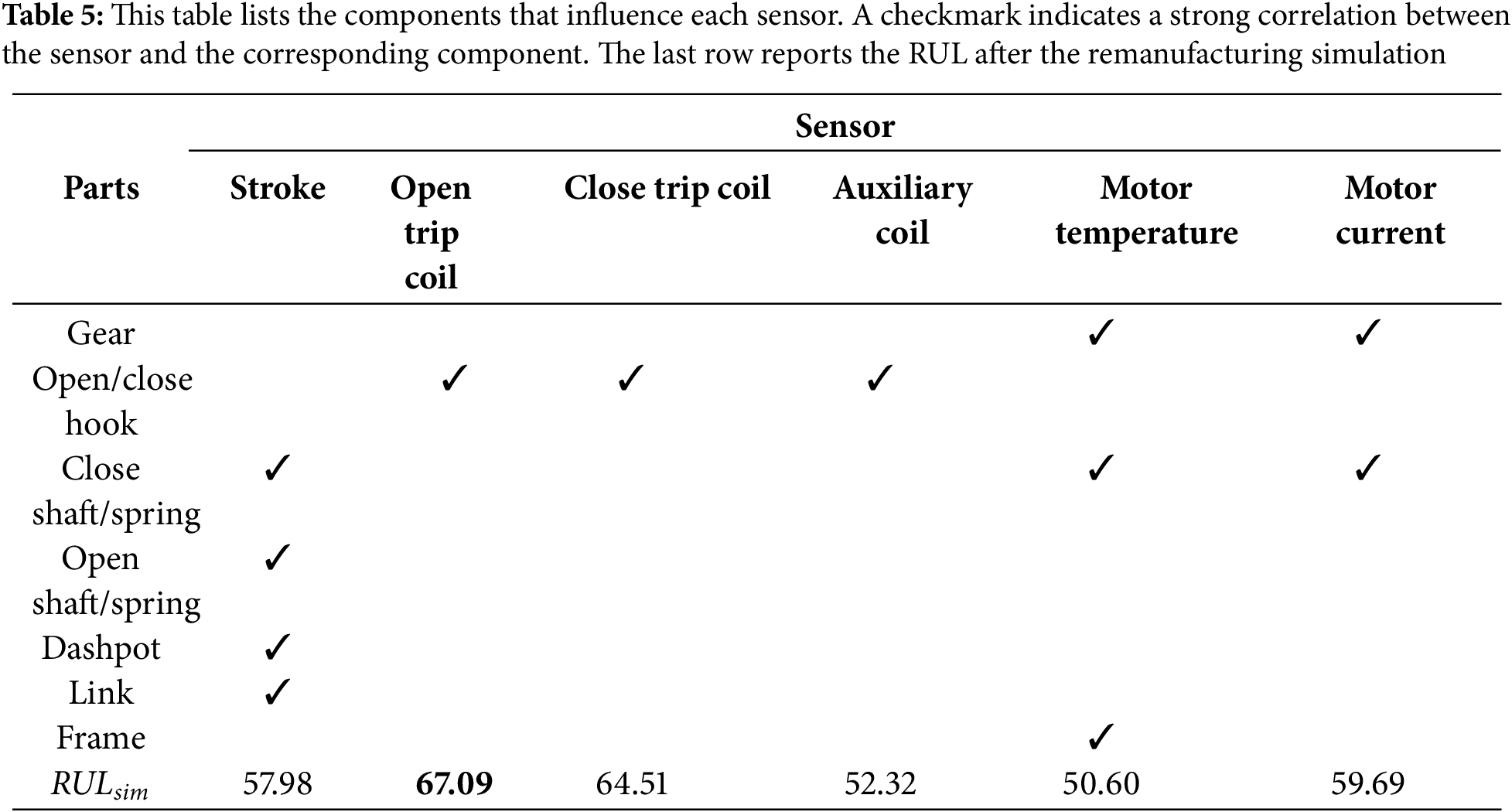
Additionally, unlike other methods, the proposed approach supports component-level decision-making. Based on expert knowledge, we established the correlation between each GIS component and its associated sensors, as summarized in Table 5. The last row reports the RUL values, as defined in Eq. (7), obtained from the remanufacturing simulation at the 53rd timestep, which was identified as the optimal remanufacturing point. Since the parameter k was set to 1, we selected the sensor with the highest post-remanufacturing RUL: the open trip coil sensor. According to the table, this sensor is strongly associated with the open/close hook component. Therefore, at the 53rd timestep, the model recommends replacing the open/close hook as the most effective remanufacturing action. Notably, this component-level decision-making capability is a distinctive feature of the proposed method and is not addressed in previous works.

4.5 Additional Analysis of Proposed Framework

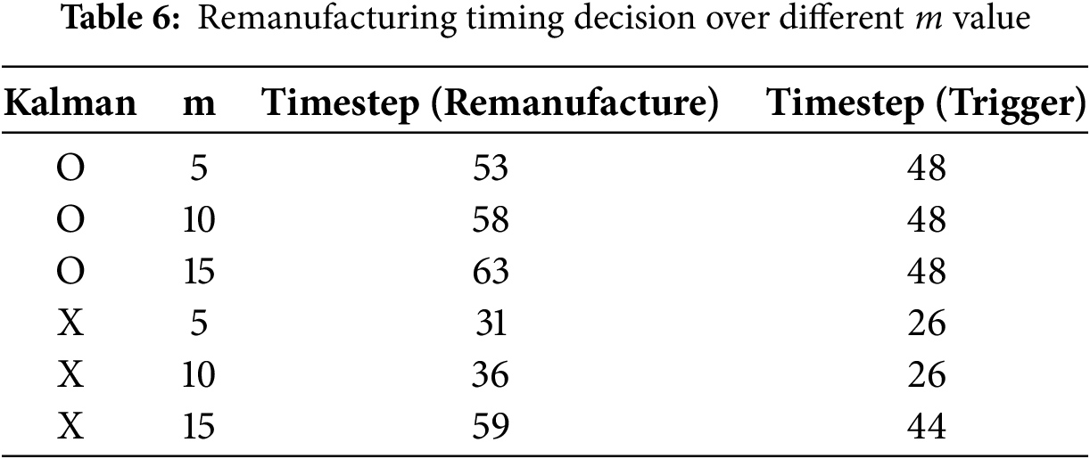
This section presents an in-depth analysis of the proposed framework, examining how user-selected parameters affect its behavior and performance. First, we focus on parameter m in Algorithm 1, a critical hyperparameter that triggers remanufacturing when the decision value fails to increase over m consecutive timesteps. Table 6 summarizes the results obtained for different values of m. The table includes whether the Kalman filter was applied, the value of m, the remanufacturing time determined by the algorithm, and the trigger time, which is computed by subtracting m from the determined remanufacturing timestep. When the Kalman filter was applied, remanufacturing was consistently triggered at the 48th timestep, regardless of the m value, indicating that the proposed framework is stable against variations in hyperparameters. In contrast, without the Kalman filter, the selected m value had a noticeable impact on the timing of the remanufacturing decision due to fluctuations caused by noise in the decision values. These results demonstrate that the Kalman filter effectively suppresses random fluctuations and prevents premature or delayed triggering, thereby improving the robustness of online decision-making under noisy sensor conditions. Furthermore, the limited variation observed across m values confirms that the overall framework remains insensitive to minor parameter changes, ensuring consistent decision performance across different operational scenarios.

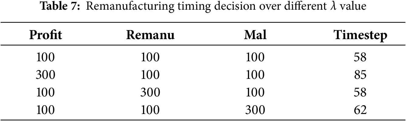
Additionally, the framework supports customization by allowing users to adjust the weights assigned to each component in the decision value calculation. Although the default configuration sets all weight parameters (λprofit, λremanu, λmal) to 100 to balance the scale of each term, these values can be freely adjusted to meet domain-specific requirements. This flexibility enables the decision-making process to reflect specific priorities, such as emphasizing profit over remanufacturing cost or malfunction risk. Fig. 10 illustrates how changes in the weight parameter λ influence the resulting decision values. Notably, increasing the profit weight (orange line) led to higher decision values than equal weights (blue line). In contrast, assigning greater weight to cost components (green and red lines) resulted in lower decision values. Table 7 summarizes how these weight adjustments affect the remanufacturing timing, demonstrating the sensitivity of the decision value to changes in weight configuration. This adaptability confirms that the framework can be fine-tuned to various operational contexts and user strategies, allowing decisions to reflect policy preferences rather than a single fixed setting.

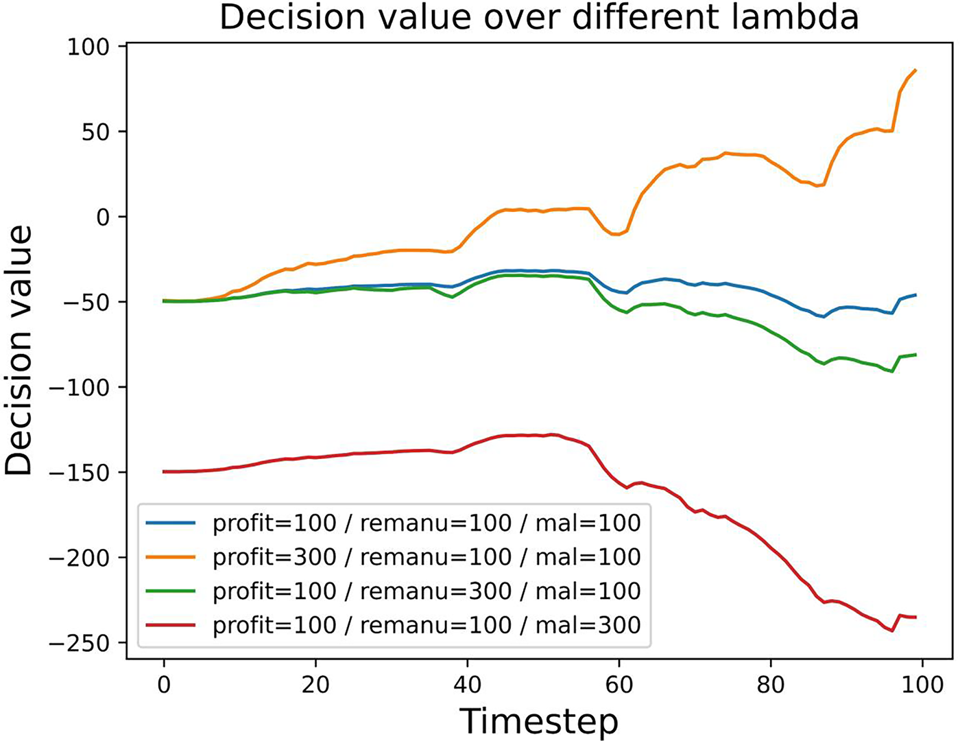
Figure 10: Calculation results of decision values over different weights

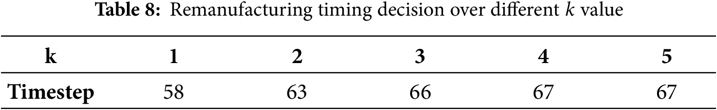
In addition to λ customization, the proposed framework enhances decision-making flexibility by allowing adjustments to k, the number of sensors selected for replacement. Although the default configuration sets k=1, which represents a single-component replacement scenario, users can freely adjust this parameter to reflect different maintenance strategies. Fig. 11a shows a positive correlation between the number of sensors replaced and the resulting profit, which increases due to the extended equipment lifetime. Fig. 11b illustrates that remanufacturing costs also rise with higher values of k, reflecting the added expense of replacing more components. In contrast, as shown in Fig. 11c, malfunction costs remain constant regardless of k, consistent with the assumptions discussed in Section 3.3. Fig. 11d highlights how the decision value adapts to changes in k, demonstrating the framework’s inherent flexibility. Using Algorithm 1, the optimal remanufacturing timing can be dynamically determined based on different k values. Table 8 illustrates the framework’s capability to support adaptive decision-making based on varying sensor replacement scales.

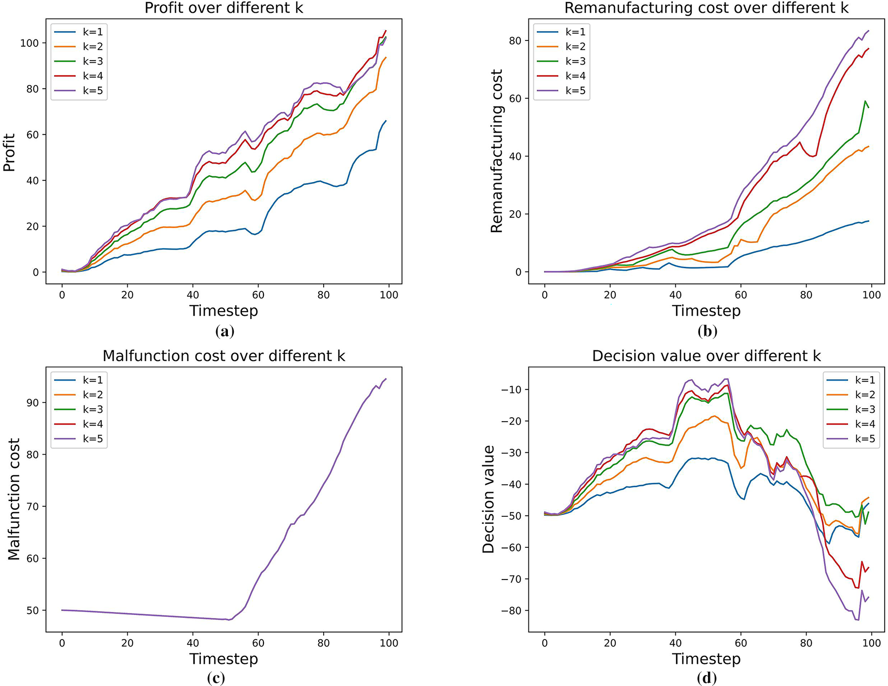
Figure 11: Calculation result of decision value and components over different k values. (a) Profit, (b) remanufacturing cost, (c) malfunction cost, and (d) decision value

In the main experiment, the RUL of GIS equipment was assumed to decrease linearly. However, the pattern of RUL degradation can vary depending on the operating environment of the GIS equipment. Therefore, to verify the robustness of the proposed framework under various RUL scenarios, we applied it to two additional scenarios with distinct RUL degradation patterns. As shown in Fig. 12a, we considered two scenarios: a late-stage degradation scenario, where the RUL decreases rapidly toward the end of the lifecycle (indicated by the red line), and an early-stage degradation scenario, where the RUL decreases rapidly at the beginning of the lifecycle (indicated by the blue line). Fig. 12b presents the results of applying the proposed framework to the late-stage degradation scenario, while Fig. 12c shows the results for the early-stage degradation scenario. In both cases, the left side of Fig. 12b and c displays the performance of the RUL prediction model, similar to Fig. 7a. The results demonstrated that the ensemble PA model achieves performance comparable to that of the RF model, confirming that the proposed framework can effectively perform online RUL prediction even under different RUL degradation scenarios. The right side of Fig. 12b and c shows the decision values calculated using the RUL prediction model. Based on the calculated decision values, Algorithm 1 was applied to determine the optimal remanufacturing timing. In the late-stage degradation scenario, remanufacturing was performed at the 67th timestep, whereas in the early-stage degradation scenario, it was performed at the 42nd timestep. These results indicate that the proposed RUL framework can accurately support decision-making across different RUL scenarios. Specifically, when RUL decreases rapidly in the early stages, remanufacturing is performed earlier, and when RUL decreases rapidly in the late stages, remanufacturing is delayed accordingly. This adaptability highlights the robustness and reliability of the proposed framework for online decision-making.

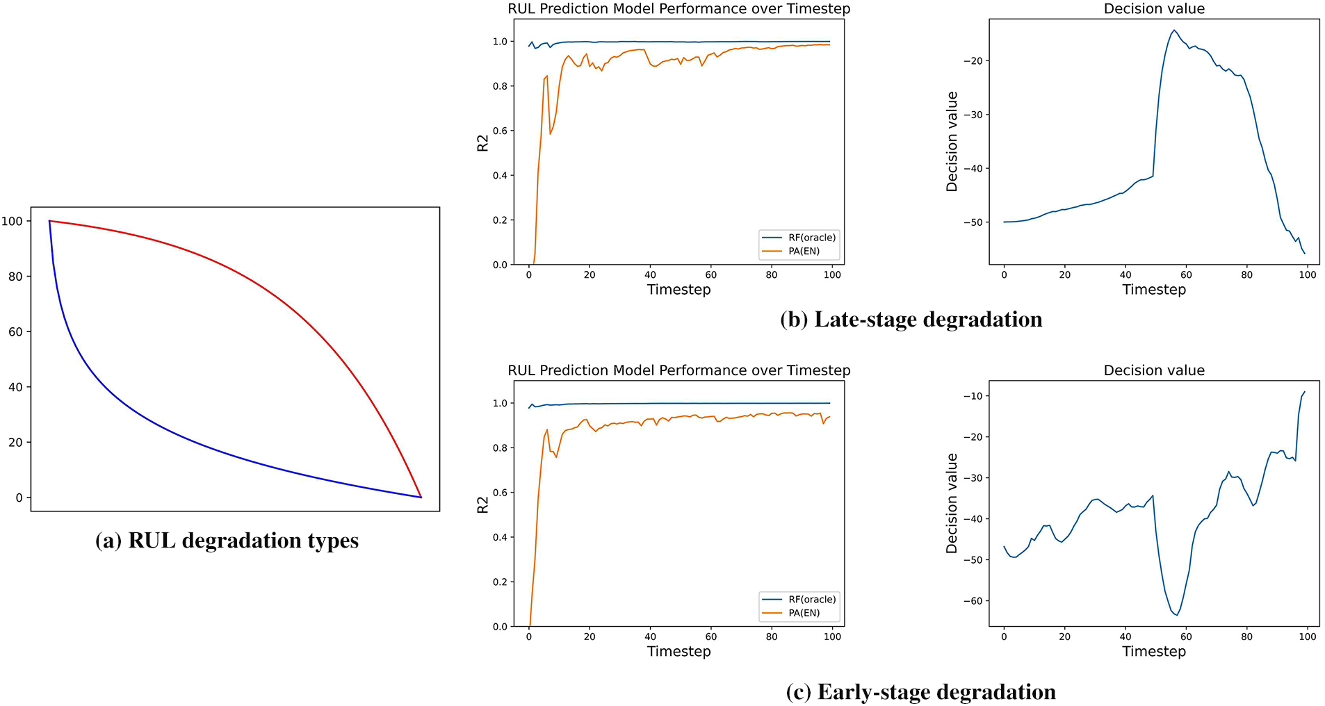
Figure 12: (a) Illustration of RUL degradation types (red: late-stage degradation, blue: early-stage degradation), (b) Results for the late-stage degradation scenario, (c) Results for the early-stage degradation scenario

To validate the extensibility of the proposed framework, we applied it to additional datasets beyond those used in the main experiment. GIS can be categorized based on the circuit breaker mechanism used to interrupt electricity. While the primary results were obtained using data collected from GIS with spring-based circuit breakers, we extended the analysis to datasets collected from GIS with hydraulic and pneumatic mechanisms. Fig. 13a shows the results for hydraulic GIS, and Fig. 13b displays the results for pneumatic GIS. The left side of Fig. 13a and b demonstrates the performance of the RUL prediction models. Unlike the spring-type dataset, the ensemble PA model exhibits significantly lower performance compared to the RF model. This indicates that for certain datasets, the online RUL prediction model may not perform as accurately. However, even in such cases, the proposed framework remains applicable. Assuming sufficient computational resources are available on the equipment, the decision-making process can be carried out using the RF model. The right side of Fig. 13a and b presents the decision values calculated based on the RF model. By using these decision values and applying Algorithm 1, the optimal remanufacturing timing was determined. For hydraulic GIS, remanufacturing was scheduled at the 61st timestep, while for pneumatic GIS, it was scheduled at the 65th timestep. These results demonstrate that the proposed framework can still be effectively applied even when the online RUL prediction model does not perform optimally. With sufficient computational resources, the framework ensures reliable decision-making, underscoring its applicability across diverse datasets.

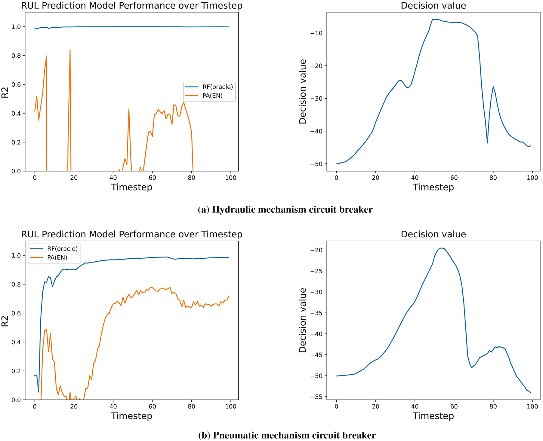
Figure 13: Performance evaluation and decision-making results for (a) hydraulic and (b) pneumatic GIS datasets

5  Discussion

The experimental results collectively demonstrate the adaptability, robustness, and practical applicability of the proposed framework. Fig. 7 illustrates the advantage of integrating online machine learning into the remanufacturing process. By continuously updating the RUL prediction model with streaming sensor data, the proposed method adapts to ongoing equipment degradation while maintaining low computational cost. Fig. 9 compares the proposed method with existing approaches. While previous methods depend on future data for optimization, the proposed framework achieves comparable decision quality using only current and past information. This confirms the framework’s ability to deliver near-optimal remanufacturing timing in realistic conditions. In addition, unlike previous approaches, the proposed framework provides component-level guidance, enabling interpretable decision-making on which parts should be replaced. As shown in Table 5, the framework successfully identifies the most effective component-level remanufacturing actions based on the contribution of each sensor to the predicted RUL improvement. Overall, these findings confirm that the proposed framework consistently delivers robust, adaptive, and interpretable remanufacturing decisions.

6  Conclusion

This study presented a data-driven, online, component-level decision-making framework for the remanufacturing of GIS. Conventional approaches that rely on predefined mathematical models and offline optimization are often impractical in real-world industrial settings. To address this limitation, the proposed framework integrates three key components: an online RUL prediction model, an online optimization algorithm, and a component-level decision-making module. Conventional frameworks that rely on offline optimization require access to complete future data, so decisions can only be made after the equipment has failed. In contrast, the proposed system employs online optimization, enabling real-time decision-making while the equipment is still operating. This allows the system to respond to ongoing degradation before complete failure occurs, supporting timely, data-driven decisions under realistic industrial conditions. Consequently, the framework functions as a real-time decision-making system that continuously evaluates equipment health, minimizes downtime, prevents unexpected failures, and ensures that remanufacturing occurs at the most cost-effective moment. Although this study focused on GIS, the proposed framework provides a generalizable methodology applicable to various types of industrial equipment that collect condition-monitoring data. One limitation of the framework is that, because the model is trained exclusively on online data, RUL predictions may be less accurate during the early stages of equipment operation. Since all decisions rely on RUL estimates, this can lead to suboptimal decision-making at the beginning of the equipment’s lifecycle. Future work will focus on improving early-stage RUL accuracy by incorporating pre-trained models or applying transfer learning from similar equipment. These enhancements aim to further improve the reliability and robustness of early-stage decision-making within the proposed framework.

Acknowledgement: None.

Funding Statement: This work was supported by the Human Resources Development of the Korea Institute of Energy Technology Evaluation and Planning (KETEP) grant funded by the Korea government Ministry of Knowledge Economy (No. RS-2023-00244330) and the National Research Foundation of Korea (NRF) grant funded by the Korea government (MSIT) (No. NRF RS-2023-00219052; RS-2024-00352587).

Author Contributions: The authors confirm contribution to the paper as follows: Conceptualization, Hansam Cho and Seokho Moon; methodology, Hansam Cho; software, Hansam Cho; validation, Hansam Cho, Seokho Moon and Sunhyeok Hwang; formal analysis, Hansam Cho; data curation, Hansam Cho, Seokho Moon and Sunhyeok Hwang; writing—original draft preparation, Hansam Cho; writing—review and editing, Hansam Cho, Seokho Moon, Sunhyeok Hwang, Seoung Bum Kim and Younghoon Kim; visualization, Hansam Cho; supervision, Seoung Bum Kim and Younghoon Kim; project administration, Younghoon Kim; funding acquisition, Seoung Bum Kim and Younghoon Kim. All authors reviewed the results and approved the final version of the manuscript.

Availability of Data and Materials: The data used in this study were collected in collaboration with industry partners and are subject to company security policies. Therefore, the dataset cannot be publicly released.

Ethics Approval: Not applicable. This study did not involve human participants or animals.

Conflicts of Interest: The authors declare no conflicts of interest to report regarding the present study.

References

1. Thierry M, Salomon M, Van Nunen J, Van Wassenhove L. Strategic issues in product recovery management. Calif Manage Rev. 1995;37(2):114–36. doi:10.2307/41165792. [Google Scholar] [CrossRef]

2. Souza GC, Ketzenberg ME, Guide VDRJr. Capacitated remanufacturing with service level constraints. Prod Oper Manage. 2002;11(2):231–48. doi:10.1111/j.1937-5956.2002.tb00493.x. [Google Scholar] [CrossRef]

3. Johnson MR, McCarthy IP. Product recovery decisions within the context of extended producer responsibility. J Eng Technol Manage. 2014;34:9–28. doi:10.1016/j.jengtecman.2013.11.002. [Google Scholar] [CrossRef]

4. Jensen JP, Prendeville SM, Bocken NM, Peck D. Creating sustainable value through remanufacturing: three industry cases. J Clean Prod. 2019;218:304–14. doi:10.1016/j.jclepro.2019.01.301. [Google Scholar] [CrossRef]

5. Seitz MA, Peattie K. Meeting the closed-loop challenge: the case of remanufacturing. Calif Manage Rev. 2004;46(2):74–89. doi:10.2307/41166211. [Google Scholar] [CrossRef]

6. Saavedra YM, Barquet AP, Rozenfeld H, Forcellini FA, Ometto AR. Remanufacturing in Brazil: case studies on the automotive sector. J Clean Prod. 2013;53:267–76. doi:10.1016/j.jclepro.2013.03.038. [Google Scholar] [CrossRef]

7. Matsumoto M, Umeda Y. An analysis of remanufacturing practices in Japan. J Remanuf. 2011;1:1–11. doi:10.1186/2210-4690-1-2. [Google Scholar] [CrossRef]

8. Kerr W, Ryan C. Eco-efficiency gains from remanufacturing: a case study of photocopier remanufacturing at Fuji Xerox Australia. J Clean Prod. 2001;9(1):75–81. doi:10.1016/S0959-6526(00)00032-9. [Google Scholar] [CrossRef]

9. Song S, Liu M, Ke Q, Huang H. Proactive remanufacturing timing determination method based on residual strength. Int J Prod Res. 2015;53(17):5193–206. doi:10.1080/00207543.2015.1012599. [Google Scholar] [CrossRef]

10. Liu Z, Afrinaldi F, Zhang HC, Jiang Q. Exploring optimal timing for remanufacturing based on replacement theory. CIRP Ann. 2016;65(1):447–50. doi:10.1016/j.cirp.2016.04.064. [Google Scholar] [CrossRef]

11. Gong Q, Xiong Y, Jiang Z, Yang J, Chen C. Timing decision for active remanufacturing based on 3E analysis of product life cycle. Sustainability. 2022;14(14):8749. doi:10.3390/su14148749. [Google Scholar] [CrossRef]

12. Ke Q, Li J, Huang H, Liu G, Zhang L. Performance evaluation and decision making for pre-decision remanufacturing timing with on-line monitoring. J Clean Prod. 2021;283:124606. doi:10.1016/j.jclepro.2020.124606. [Google Scholar] [CrossRef]

13. Haque TS, Chakraborty A, Alam S. E-learning app selection multi-criteria group decision-making problem using Einstein operator in linguistic trapezoidal neutrosophic environment. Knowl Inf Syst. 2025;67(3):2481–519. doi:10.1007/s10115-024-02265-6. [Google Scholar] [CrossRef]

14. Banik B, Chakraborty A, Barman A, Alam S. Multi-method approach for new vehicle purchasing problem through MCGDM technique under cylindrical neutrosophic environment. Soft Comput. 2024;4:1–17. doi:10.1007/s00500-023-09520-y. [Google Scholar] [CrossRef]

15. Dong L, Dai Y. Research on alliance decision of dual-channel remanufacturing supply chain considering bidirectional free-riding and cost-sharing. Comput Model Eng Sci. 2024;140(3):2913. doi:10.32604/cmes.2024.049214. [Google Scholar] [CrossRef]

16. Zhou Y, Lin XT, Fan ZP, Wong KH. Remanufacturing strategy choice of a closed-loop supply chain network considering carbon emission trading, green innovation, and green consumers. Int J Environ Res Public Health. 2022;19(11):6782. doi:10.3390/ijerph19116782. [Google Scholar] [PubMed] [CrossRef]

17. Yi P, Huang M, Guo L, Shi T. A retailer oriented closed-loop supply chain network design for end of life construction machinery remanufacturing. J Clean Prod. 2016;124:191–203. doi:10.1016/j.jclepro.2016.02.070. [Google Scholar] [CrossRef]

18. Yang S, Nasr N, Ong S, Nee A. A holistic decision support tool for remanufacturing: end-of-life (EOL) strategy planning. Adv Manuf. 2016;4:189–201. doi:10.1007/s40436-016-0149-2. [Google Scholar] [CrossRef]

19. Liao H, Li C, Nie Y, Tan J, Liu K. Environmental efficiency assessment for remanufacture of end of life machine and multi-objective optimization under carbon trading mechanism. J Clean Prod. 2021;308:127168. doi:10.1016/j.jclepro.2021.127168. [Google Scholar] [CrossRef]

20. Moon S, Cho H, Koh E, Cho YS, Oh HL, Kim Y, et al. Remanufacturing decision-making for gas insulated switchgear with remaining useful life prediction. Sustainability. 2022;14(19):12357. doi:10.3390/su141912357. [Google Scholar] [CrossRef]

21. da Costa PRDO, Akçay A, Zhang Y, Kaymak U. Remaining useful lifetime prediction via deep domain adaptation. Reliab Eng Syst Saf. 2020;195:106682. doi:10.1016/j.ress.2019.106682. [Google Scholar] [CrossRef]

22. Chen Z, Wu M, Zhao R, Guretno F, Yan R, Li X. Machine remaining useful life prediction via an attention-based deep learning approach. IEEE Trans Ind Electron. 2020;68(3):2521–31. doi:10.1109/TIE.2020.2972443. [Google Scholar] [CrossRef]

23. Yan J, He Z, He S. A deep learning framework for sensor-equipped machine health indicator construction and remaining useful life prediction. Comput Ind Eng. 2022;172:108559. doi:10.1016/j.cie.2022.108559. [Google Scholar] [CrossRef]

24. Li Y, Kurfess T, Liang S. Stochastic prognostics for rolling element bearings. Mech Syst Signal Process. 2000;14(5):747–62. doi:10.1006/mssp.2000.1301. [Google Scholar] [CrossRef]

25. Banjevic D, Jardine A. Calculation of reliability function and remaining useful life for a Markov failure time process. IMA J Manage Math. 2006;17(2):115–30. doi:10.1093/imaman/dpi029. [Google Scholar] [CrossRef]

26. Wang SH, Kang X, Wang C, Ma TB, He X, Yang K. A hybrid approach for predicting the remaining useful life of bearings based on the RReliefF algorithm and extreme learning machine. Comput Model Eng Sci. 2024;140(2):1405. doi:10.32604/cmes.2024.049281. [Google Scholar] [CrossRef]

27. Peng W, Ye ZS, Chen N. Joint online RUL prediction for multivariate deteriorating systems. IEEE Trans Ind Informat. 2018;15(5):2870–8. doi:10.1109/TII.2018.2869429. [Google Scholar] [CrossRef]

28. Wang FK, Amogne ZE, Chou JH, Tseng C. Online remaining useful life prediction of lithium-ion batteries using bidirectional long short-term memory with attention mechanism. Energy. 2022;254:124344. doi:10.1016/j.energy.2022.124344. [Google Scholar] [CrossRef]

29. Zhuang J, Cao Y, Jia M, Zhao X, Peng Q. Remaining useful life prediction of bearings using multi-source adversarial online regression under online unknown conditions. Expert Syst Appl. 2023;227:120276. doi:10.1016/j.eswa.2023.120276. [Google Scholar] [CrossRef]

30. Crammer K, Dekel O, Keshet J, Shalev-Shwartz S, Singer Y. Online passive-aggressive algorithms. J Mach Learn Res. 2006;7:551–85. [Google Scholar]

31. Liu C, Chen J, Cai W. Data-driven remanufacturability evaluation method of waste parts. IEEE Trans Ind Informat. 2021;18(7):4587–95. doi:10.1109/TII.2021.3118466. [Google Scholar] [CrossRef]

32. Taguchi G. Introduction to quality engineering: designing quality into products and processes. Tokyo, Japan: Asian Productivity Organization; 1986. [Google Scholar]

33. Qin S, Wang BX, Wu W, Ma C. The prediction intervals of remaining useful life based on constant stress accelerated life test data. Eur J Oper Res. 2022;301(2):747–55. doi:10.1016/j.ejor.2021.11.026. [Google Scholar] [CrossRef]

34. Han D, Bai T. Design optimization of a simple step-stress accelerated life test—contrast between continuous and interval inspections with non-uniform step durations. Reliab Eng Syst Saf. 2020;199:106875. doi:10.1016/j.ress.2020.106875. [Google Scholar] [CrossRef]

35. Bhattacharjee P, Dey V, Mandal U. Risk assessment by failure mode and effects analysis (FMEA) using an interval number based logistic regression model. Saf Sci. 2020;132:104967. doi:10.1016/j.ssci.2020.104967. [Google Scholar] [CrossRef]

36. Fu S, Cheng F, Tjahjowidodo T, Zhou Y, Butler D. A non-contact measuring system for in-situ surface characterization based on laser confocal microscopy. Sensors. 2018;18(8):2657. doi:10.3390/s18082657. [Google Scholar] [PubMed] [CrossRef]

37. Ren L, Zhao L, Hong S, Zhao S, Wang H, Zhang L. Remaining useful life prediction for lithium-ion battery: a deep learning approach. IEEE Access. 2018;6:50587–98. doi:10.1109/ACCESS.2018.2858856. [Google Scholar] [CrossRef]

38. Liu Y, Liu J, Wang H, Yang M, Gao X, Li S. A remaining useful life prediction method of mechanical equipment based on particle swarm optimization-convolutional neural network-bidirectional long short-term memory. Machines. 2024;12(5):342. doi:10.3390/machines12050342. [Google Scholar] [CrossRef]

39. Ge X, Fan Y, Li J, Wang Y, Deng S. Noise reduction of nuclear magnetic resonance (NMR) transversal data using improved wavelet transform and exponentially weighted moving average (EWMA). J Magn Reson. 2015;251:71–83. doi:10.1016/j.jmr.2014.11.018. [Google Scholar] [PubMed] [CrossRef]

40. Breiman L. Random forests. Mach Learn. 2001;45:5–32. doi:10.1023/A:1010933404324. [Google Scholar] [CrossRef]

41. Kalman RE. A new approach to linear filtering and prediction problems. J Basic Eng. 1960;82(1):35–45. doi:10.1115/1.3662552. [Google Scholar] [CrossRef]