EventTracker Based Regression Prediction with Application to Composite Sensitive Microsensor Parameter Prediction

1  Introduction

With the advancement of technology, significant challenges have been presented to understanding and predicting the behavior of complex systems due to their high dynamism, uncertainty, and nonlinearity. Sensitivity Analysis (SA) [1,2], as an effective method for revealing the impact of input variables on system outputs, allows the identification of the most critical factors influencing system behavior by decision-makers.

However, traditional SA methods, including regression-based, distribution-based, and heuristic approaches, are often reliant on historical data or expert knowledge. Efficiency may be compromised when large-scale real-time data is handled, particularly in highly dynamic systems where limitations become more evident. For example, regression-based methods [3,4], although capable of inferring sensitivity information through model fitting, typically require numerous preset rules and may be constrained by linear assumptions in global sensitivity analysis. Distribution-based methods [3,5], despite their focus on the distribution characteristics of outputs, also necessitate predefined rules. Furthermore, heuristic methods [6], while able to provide quick solutions in certain scenarios, are generally based on empirical rules and may lack a comprehensive understanding of system behavior. Previous studies have demonstrated that this limitation also manifests in complex engineering systems. In high-penetration wind power grids, for example, rapid fluctuations in primary energy significantly compromise transient stability. Tina et al. [7] conducted parameter sensitivity analyses to evaluate the effects of turbine location and generation capacity on system stability. However, their results indicated that such analyses alone are insufficient to ensure robustness under disturbances, and that dynamic control measures—such as STATCOM, SVC, or fast excitation systems—remain indispensable. These findings underscore that in highly dynamic, event-driven environments, conventional sensitivity analysis fails to adequately capture or address the system’s rapid transient responses.

To address these challenges, a real-time sensitivity analysis method based on event clustering techniques [8] has been introduced. This approach eliminates the reliance on historical data or preset rules by swiftly identifying key influencing factors through the real-time analysis of dynamic relationships between input and output variables. This capability enables the dynamic monitoring of system state changes and provides essential sensitivity information for predictive models.

To achieve effective prediction in complex systems, this study integrates an event-based real-time sensitivity analysis method with machine learning models, with particular emphasis on the Light Gradient Boosting Machine (LightGBM) [9–11]. The event-based real-time sensitivity analysis method captures and quantifies the contribution of input variables to system outputs in real time, thereby providing the foundation for feature weighting. However, this approach often considers only the direct influence of inputs on outputs, while overlooking correlations and redundancies among input variables. To address this limitation, mutual information (MI) [12,13] is incorporated into the event-driven feature strength metric to quantify inter-feature dependencies. The resulting weights serve as a basis for subsequent feature evaluation, helping to mitigate the interference of redundant features and enhance both the interpretability and robustness of the predictive model.

In predictive modeling, a wide range of regression algorithms have been applied to complex system modeling, each with its own strengths and limitations. For example, Ridge Regression [14] and ElasticNet Regression [15] are effective in mitigating multicollinearity, yet their performance is limited when addressing highly nonlinear problems. Support Vector Regression (SVR) [16,17] demonstrates strong capability in handling high-dimensional and nonlinear data; however, it is highly sensitive to kernel choice and parameter tuning, and its computational efficiency can deteriorate when applied to large-scale datasets. XGBoost [18] and its histogram-based variant (XGBoost-hist) offer superior efficiency in large-scale data processing, but their performance depends on careful and often complex hyperparameter optimization. CatBoost [19] excels in dealing with categorical features but typically incurs high computational costs. The HistGradientBoosting Regressor [20] performs well on small- to medium-sized datasets, though its interpretability remains limited. Tobit regression [21,22] is good at handling nonlinear input-output correlations but needs certain approximation on probability density function computation. In comparison, LightGBM leverages an efficient histogram-based algorithm and a leaf-wise growth strategy, providing notable advantages in both training speed and predictive accuracy.

The main contributions of this study can be summarized as follows:

1.   Integration of event-driven real-time sensitivity analysis with mutual-information weighting, enabling robust and redundancy-aware feature selection that captures both the dynamic influence of input variables and their interdependencies.

2.   Development of an adaptive iterative threshold optimization strategy guided by predictive accuracy, where LightGBM serves as the prediction model and the optimal threshold is adaptively determined across candidate values.

3.   First application of the proposed framework to composite microsensor data, demonstrating efficient and robust real-time prediction and highlighting its potential for practical industrial monitoring.

These innovations not only introduce new approaches to sensitivity analysis and predictive modeling but also validate their robustness and efficiency for real-time prediction through experiments on composite microsensor data, thereby demonstrating strong potential for industrial monitoring applications.

2  Methodology

The overall procedure of the proposed method is illustrated in Fig. 1, where the framework is jointly constructed by the EventTracker method and the LightGBM regression model. The event-based sensitivity analysis decomposes system states into a sequence of discrete events triggered by changes in input variables, without the need to predefine system states or rely on historical events. This enables near real-time characterization of the relationship between system states and inputs. Building upon this foundation, we further compute prior weights for the input features to quantitatively evaluate their contributions to the output.

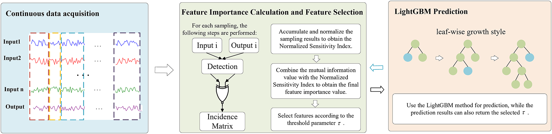
Figure 1: The schematic diagram illustrates the overall method

Specifically, we first introduce the configuration of trigger thresholds and event thresholds in the EventTracker method, which are determined by a combination of system characteristics and expert knowledge. We then describe how continuous data are transformed into discrete events and illustrate how this process facilitates real-time monitoring of system state changes. In the feature selection stage, event-driven sensitivity measures are employed to compute the strength of each feature, while mutual information (MI) is incorporated to suppress redundancy, thereby producing prior weights that account for both contribution and independence. Based on these weights, the Progressive Cumulative Importance Selection (PG-CIS) method is applied to filter features, and iterative threshold optimization is performed to identify the final set of key features. Finally, LightGBM is employed to construct the predictive model, enabling efficient modeling and accurate prediction of complex systems.

2.1 EventTracker Method

As shown in Fig. 2, the EventTracker method converts the continuous data analysis of a dynamic system into the dynamic monitoring of a set of discrete events, facilitating real-time response to changes in system state and quantification of sensitivity. This simplifies the real-time monitoring and analysis of complex systems. An “event” is defined as a significant transition in system state, which can be observed as sharp fluctuations in sensor readings, adjustments in operational conditions, or notable variations in system performance.

Figure 2: The EventTracker method

2.1.1 Detection

The purpose of this step is to identify Triggered and Event Data. At each sampling step, the absolute change of the input and output relative to their immediately preceding values is computed. If the change in the input exceeds the Triggered Threshold (TT), the current sample is classified as Triggered Data; likewise, if the change in the output exceeds the Event Threshold (ET), it is classified as Event Data. Formula (4) formalizes this rule.

if |Inputt−Inputt−1|≥TT→Inputt=Triggerif |Outputt−Outputt−1|≥ET→Outputt=Event(1)

In practice, both the Triggered Threshold (TT) and Event Threshold (ET) are defined as three times the standard deviation of the first-order differences in historical data, following the conventional “3σ rule” to distinguish meaningful signals from noise. The detection process employs an asynchronous point-by-point sampling strategy, where each sample is compared with the previous one rather than with a fixed window. To suppress random fluctuations, an input or output sequence is classified as Triggered Data (TD = 1) or Event Data (ED = 1) only when two consecutive samples simultaneously exceed the thresholds.

2.1.2 Formation of the Incidence Matrix

To facilitate the subsequent identification of the relationship between inputs and outputs, input Data and output Data are associated through an expression similar to the exclusive OR (XOR) operation. When Input Data and Output Data are both identified as Triggered Data and Event Data, or when neither of them is identified as Triggered Data and Event Data, a value of 1 is assigned to the corresponding entry in the association matrix; otherwise, it is assigned as 0. In essence, association is considered only when Input Data and Output Data undergo the same changes.

2.1.3 Normalized Sensitivity Index Calculation

Following each sampling iteration, an Incidence Matrix is produced. Within this matrix, we substitute all 0 values with −1 to enhance the sensitivity analysis by yielding more discernible upper and lower bounds. This substitution strategy amplifies the model’s responsiveness to alterations in input variables, thereby enabling a clearer illustration of each variable’s impact during sensitivity analysis. The ultimate computation formulas are illustrated in (2) and (3).

SIt=∑1tIncidenceMatrixScores(2)

t represents the current sampling instance.

NSI=SIn−μσ(3)

where, SIn denotes the sensitivity index at the n-th sampling instance, while μ and σ represent the mean and standard deviation of all SI values across the sampling instances, respectively. This Z-score normalization ensures feature comparability and eliminates the influence of scale differences.

2.2 Input Variables Importance Calculation

2.2.1 Mutual Information

Mutual Information (MI) is a fundamental metric in information theory that quantifies the amount of information gained about one variable through the observation of another. For two random variables, MI measures the reduction in uncertainty of one variable given knowledge of the other, typically expressed in bits. The MI definition is as shown in (4). MI is widely used to quantify the dynamic information exchange between candidate features and the target variable—whether categorical or continuous—serving as an effective measure of feature relevance.

MI(X;Y)=∑x∈X∑y∈Yp(x,y)log⁡p(x,y)pX(x)pY(y)(4)

where x and y represent the attribute values of the variables X and Y, respectively, pX(x) and pY(y) represent the edge probability distribution, p(x,y) represents the joint probability distribution. Mutual Information (MI) intuitively measures the information shared between X and Y, reflecting the reduction in uncertainty of one variable when the other is known. For instance, if X and Y are independent, no information about Ycan be obtained from X, and vice versa, resulting in an MI value of zero. A higher MI(X;Y) signifies a stronger dependence between X and Y.

In this study, we adopt a histogram-based estimation approach to compute MI. Specifically, continuous variables are discretized using a label-encoding scheme, after which the marginal and joint probability distributions are estimated by frequency counts. The MI values are then obtained using the definition in (4).

2.2.2 Input Variables Importance Calculation

The EventTracker method quantifies the contribution of each input to the output. However, the raw EventTracker outputs can take both positive and negative signs, which makes them unsuitable for direct interpretation as importance weights. To obtain a sign-invariant and comparable magnitude of contribution, we first convert the EventTracker outputs into a strength measure by taking the mean absolute value within each window and then normalizing across features. In addition, EventTracker focuses solely on input–output relationships and overlooks interdependencies among inputs; therefore, we further incorporate a redundancy-aware adjustment based on mutual information (MI).

Let Z∈RT×n denote the (signed) EventTracker outputs after normalization along the time axis, where T is the total number of time steps and n is the number of input variables. The strength of the i-th input is defined as the mean absolute value:

S~X[:,i] = 1T∑t=1T|Z(t,i)|.(5)

To ensure comparability across features, we scale the strengths into [0,1] by max-normalization:

SX[:,i] = S~X[:,i]maxk∈{1,…,n}S~X[:,k].(6)

To account for inter-feature redundancy, we employ mutual information (MI) among input variables. The redundancy of the i-th input is quantified by the average MI it shares with all other inputs:

MI_Sumi = ∑j≠iMI(X[:,i];X[:,j]),(7)

MI¯X[:,i] = MI_Sumin−1.(8)

We then directly define the independence score by applying min–max normalization to the averaged mutual information values.

IndX[:,i] = MI¯X[:,i]−minkMI¯X[:,k]maxkMI¯X[:,k]−minkMI¯X[:,k],(9)

The preliminary score combines the sign-invariant strength and the independence:

ScoreX[:,i] = SX[:,i] + IndX[:,i].(10)

Finally, to ensure non-negativity and cross-feature comparability, we apply min–max normalization to obtain the final importance:

ImpX[:,i] = ScoreX[:,i]−minkScoreX[:,k]maxkScoreX[:,k]−minkScoreX[:,k].(11)

2.3 Predictive Models and Threshold Selection

2.3.1 Prediction Model

In this study, LightGBM (Light Gradient Boosting Machine) is adopted as the predictive model. LightGBM belongs to the family of gradient boosting decision tree (GBDT) algorithms, in which the central principle is to iteratively fit new regression trees to the residuals of the preceding model, thereby progressively enhancing prediction accuracy. Unlike traditional GBDT implementations, LightGBM incorporates a histogram-based splitting algorithm together with a leaf-wise tree growth strategy. These innovations not only markedly accelerate the training process but also help mitigate the risk of overfitting, offering a favorable balance between computational efficiency and predictive performance.

Formally, the prediction function of LightGBM can be expressed as an additive ensemble of M regression trees:

FM(x)=∑m=1Mfm(x),fm∈ℱ,(12)

where fm(⋅) denotes the m-th regression tree and ℱ is the space of all possible regression trees. In each iteration, a new tree fm is trained based on the gradients of the loss function and then added to the model.

For the regression task considered in this work, Root Mean Squared Error (RMSE) is used as the loss function to guide model training.

2.3.2 Threshold Selection

In this study, feature subsets are determined using a Prior-Guided Cumulative Importance Selection (PG-CIS) strategy. Specifically, all input features are first ranked in descending order by their prior weights, after which the cumulative weight ratio is computed along the ranked list. Once the cumulative weight exceeds a candidate threshold τ, the corresponding prefix subset of features is selected; if fewer than two features are included, the subset is expanded to at least two dimensions to ensure stability. Candidate thresholds are chosen from {0.5,0.6,0.7,0.8,0.9,0.93,0.95,0.98,1.0}. For each τ, a LightGBM regression model is trained with the selected features and autoregressive (AR) lag terms. Model performance is evaluated using root mean squared error (RMSE), mean absolute error (MAE), and coefficient of determination (R2). The threshold τ that achieves the lowest RMSE on the test set is selected as the final configuration. The PG-CIS process can be summarized as follows (Algorithm 1):

3  Case Study

In this experiment, data from composite sensitive microsensor are collected under static conditions at room temperature. The dataset includes measurements of temperature, pressure, tri-axial acceleration, and tri-axial angular velocity. The primary acquisition platform consisted of a PC equipped with Vofa software. During the acquisition process, two sensors are placed on a horizontal surface and connected to the PC via serial cables. The Vofa serial monitoring tool is then used to record tri-axial angular velocity, tri-axial acceleration, temperature, and pressure data. Through the real-time curve interface of the software, variations in the sensor outputs could be observed.

In the recorded data, I0, I1, and I2 correspond to the accelerations along the x-axes, y-axes, and z-axes, respectively, with units of g. Similarly, I3, I4, and I5 denote the angular velocities along the x-axes, y-axes, and z-axes, respectively, with units of ∘/s. I6 and I7 represent the environmental temperature (in °C) and pressure (in MPa).

The output rate (i.e., the time interval between two consecutive packets) and the measurement ranges of the sensors are summarized in Table 1. It is worth noting that the underlying acquisition hardware operated at a sampling frequency of 400 Hz, while the effective output rate is limited to 100 Hz (i.e., one data packet every 10 ms) due to the built-in down-sampling mechanism. Therefore, the acceleration and angular velocity channels provide 100 Hz data, whereas the pressure and temperature channels provide 16.7 and 3.3 Hz data, respectively. The host computer interface of the acquisition system and the physical prototype of the composite sensitive microsensor are illustrated in Figs. 3 and 4, respectively.

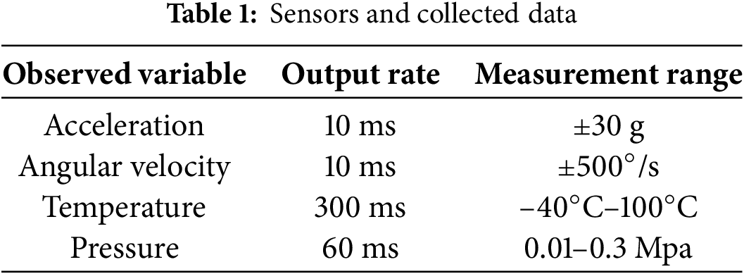
Figure 3: Host computer interface for data acquisition and monitoring

Figure 4: Photograph of the composite sensitive microsensor

In this study, a total of 247,774 data samples are collected, of which 80% are used as the training set and 20% as the test set. Within the training set, the last 10% is further reserved as the validation set. And the y-axis angular velocity (I4) is selected as the output variable, while the remaining variables are used as input features.

The experiments are performed on a computer with the following specifications: CPU: R7-6800H, Operating System: Windows 11, RAM: 32 GB, and Software: Python 3.9. The main libraries used in this study are scikit-learn 1.7.1 (for machine learning algorithms and mutual information estimation via the histogram-based method implemented in mutual_info_score) and LightGBM 4.6.0. Each algorithm in this study is independently repeated 20 times, and the simulation results are evaluated using the following performance metrics. Each algorithm in this study is independently repeated 20 times, and the simulation results are assessed using the following performance metrics.

Root Mean Square Error (RMSE)

The root mean squared error between yi and yi^ in the test dataset is calculated as follows:

RMSE=1N∑i=1N(yi−y^i)2(13)

where N represents the number of samples in the test dataset, yi denotes the actual value, and y^i represents the predicted value.

Coefficient of Determination(R2)

The degree to which the regression model explains the variance of the dependent variable is measured, ranging from 0 to 1, where 1 indicates a perfect fit to the data, and 0 signifies that the model fails to explain any variation in the dependent variable.

R2=1−∑i=1N(yi−y^i)2∑i=1N(yi−y¯)2(14)

where y¯ is the mean of yi.

Mean Absolute Error (MAE)

The mean difference between the predicted value y^i and the actual value yi is measured, representing the average prediction error of the model.

MAE=1N∑i−1N|yi−y^i|(15)

Time

The total training and prediction time.

3.1 Data Processing

Prior to model construction, the raw sensor data are preprocessed to remove invalid entries and replace missing values with the column-wise median. No additional normalization or scaling is applied, and the original physical units of each variable are preserved to maintain interpretability. To fully exploit the temporal dependence of the output variable, this study incorporates autoregressive (AR) lag features into all experiments. Specifically, several historical lag terms of the output variable I4 (e.g., I4t−1,I4t−2,I4t−3) are appended to the original input feature set as additional predictors. This design is motivated by two considerations. On the one hand, composite sensitive microsensor outputs typically exhibit stationarity and strong autocorrelation in time series, such that the current angular velocity is highly correlated with its historical values. On the other hand, when external input features are insufficient to explain short-term fluctuations, AR features can provide supplementary dynamic information of the target variable, thereby improving both the stability and accuracy of prediction. Therefore, in this study, AR features are regarded as a general augmentation strategy and are incorporated together with the input variables into subsequent feature selection and model construction processes.

3.2 Analysis of Variable Importance Results

According to the results of variable importance shown in Fig. 5, I5 exerts the most pronounced influence on the prediction, followed by I3 and I6, both of which exhibit relatively high strength and independence. The contributions of I0 and I1 are moderate. In contrast, I2 shows zero importance and thus provides virtually no predictive value.

Figure 5: Calculated values of variable importance

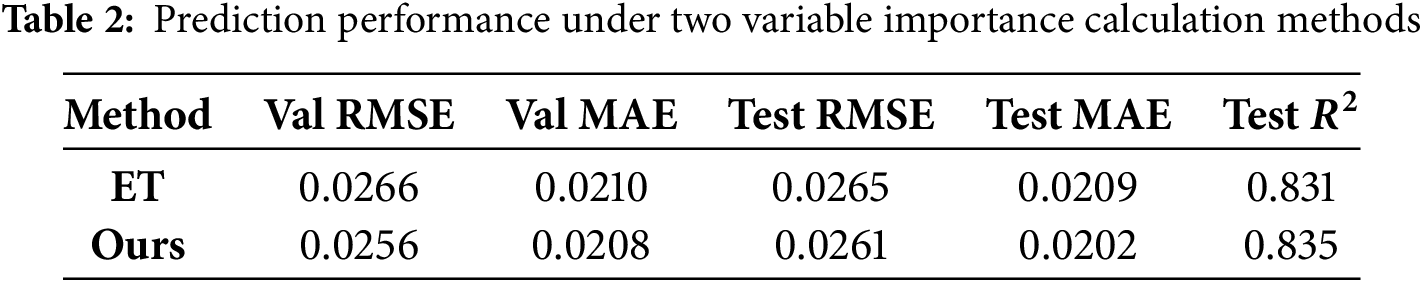
In this study, two approaches to variable importance evaluation are employed: (i) the variable importance derived solely from the EventTracker method, and (ii) the proposed method that integrates EventTracker with mutual information (MI). Under the same threshold condition (e.g., τ=0.6), the selected feature subsets differed: the former yielded [“I5”, “I3”, “I7”], whereas the latter produced [“I5”, “I3”, “I7”]. Table 2 presents a comparison of the prediction results obtained from these two methods at the given threshold. As shown, the incorporation of MI into the variable importance calculation leads to superior predictive accuracy. It is worth noting, however, that the overall error metrics are relatively small and the differences across methods remain modest. This is primarily because the experimental data are collected under static conditions at room temperature, where the variation in sensor readings is minimal, thereby limiting the observable performance differences among models.

3.3 Analysis of Predictive Performance

In this study, the value of τ is systematically varied over the range [0.5, 0.6, 0.7, 0.8, 0.9, 0.95, 0.98, 1]. For each τ, the optimal model parameters are identified using a grid-search procedure, and the corresponding sets of selected variables are summarized in Table 3. The predictive performance obtained under different τ values is presented in Fig. 6, demonstrating how the choice of τ influences overall model accuracy. It can be observed that the overall performance differences across τ values are relatively small; however, the model achieves its best performance at τ=0.5, where both the RMSE and MAE on the validation and test sets reach their lowest values, while the corresponding R2 attains its highest level. These results suggest that the feature subset selected at this threshold achieves a favorable balance between relevance and redundancy, thereby enhancing the model’s generalization capability. In contrast, when τ is set too high or too low, the feature selection becomes less appropriate, leading to a slight decline in predictive accuracy.

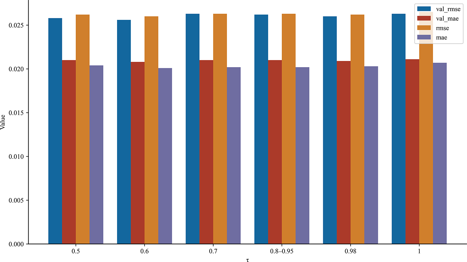
Figure 6: RMSE and MAE values for validation and testing sets at different τ

As shown in Fig. 7, the overall trend of the predicted values closely aligns with that of the ground truth, with both curves nearly overlapping across the entire sample range, except for minor deviations at a few local positions. This indicates that the predictive model performs well in capturing both the data distribution and dynamic characteristics, thereby providing an accurate approximation of the true values. Although slight fluctuations and dispersion can still be observed under large-sample conditions, the prediction curve generally succeeds in tracking the variations of the ground truth, confirming the effectiveness and stability of the proposed model.

Figure 7: True vs Predicted values

3.4 Comparison of Different Prediction Models

As shown in Table 4, the differences in RMSE and MAE across various methods on both the validation and test sets are minimal, indicating that the overall predictive accuracies are comparable. Among them, Ridge and ElasticNet achieve slightly better accuracy, while the proposed method (Ours) attains the lowest RMSE and MAE, demonstrating the most stable performance. In contrast, ensemble-based methods (HistGradientBoosting, CatBoost, and XGBoost) generally incur higher computational costs, with CatBoost in particular exhibiting a substantial time overhead, whereas linear models such as Ridge and ElasticNet are the most efficient. Considering both predictive accuracy and computational efficiency, the proposed method achieves a favorable balance, delivering high accuracy while maintaining superior efficiency, thereby underscoring its practicality and robustness.

Since the data used in this study are collected under static conditions at room temperature, the overall variability is relatively limited. To simulate nonlinear disturbance effects commonly observed in practical systems, we constructed quadratic terms, interaction terms, and periodic components based on standardized exogenous features, and superimposed them onto the original observations using the standard deviation of the target variable as the scaling factor. By gradually increasing the disturbance intensity, the adaptability and robustness of the model under different levels of nonlinear complexity can be systematically evaluated. Specifically, the selected exogenous features from the training segment are first standardized (zero mean and unit variance), after which nonlinear composite terms are generated. These composite terms include typical quadratic, interaction, and periodic components, as well as higher-order weak nonlinear terms. To ensure comparability of disturbance intensity across different experiments, the nonlinear composites are further normalized to unit variance.

As shown in (16), the standard deviation of the aligned target sequence y, denoted as σy, is employed as the disturbance scale. Disturbance terms are then superimposed on both the training and test sets of y, thereby yielding the formulation of the nonlinear perturbation:

y′=y+s⋅σy⋅term,(16)

where, s denotes the disturbance intensity coefficient, selected from the set 0.1,0.2,0.3,0.4,0.5,0.6,0.7. As s increases, the nonlinear effects become progressively stronger. For each disturbance intensity, model training and testing are conducted independently, thereby enabling a systematic evaluation of the model’s performance and stability under varying degrees of nonlinearity.

By comparing the RMSE results of LightGBM, Ridge regression, and ElasticNet under optimal parameter configurations and varying disturbance intensities (as shown in Fig. 8), several observations can be made. The RMSE curve of LightGBM remains almost flat, with only a slight increase under high-intensity disturbances, demonstrating its strong robustness against nonlinear interference. In contrast, the RMSE of Ridge regression gradually increases with disturbance intensity, exhibiting an approximately linear upward trend. This indicates that Ridge regression is more sensitive to nonlinear disturbances, although the overall growth rate remains relatively moderate. ElasticNet shows the weakest performance, with its RMSE rising sharply as the disturbance intensity increases, suggesting that it is the least adaptive when confronted with complex nonlinear components.

Figure 8: Performance comparison under different nonlinear intensities

In a unified evaluation pipeline, we compare four approaches to feature importance—TreeSHAP, Sobol indices (total-effect ST), permutation importance, and the proposed method. The first three are inherently model-based: SHAP decomposes contributions with respect to a trained predictor and its background distribution; permutation importance quantifies the drop in predictive performance when individual features are permuted; and data-driven Sobol analysis typically requires fitting a surrogate model followed by intensive sampling. By contrast, the proposed method is model-agnostic: it derives feature salience directly from the data’s event–response structure.

To ensure strict comparability, we fixed the dataset size and kept the LightGBM hyperparameter search space identical across all methods. Table 5 reports each method’s feature ranking, the optimal selection threshold τ, and the corresponding subset of chosen variables. As shown, the proposed method and permutation importance converged on the same subset, I5, I3. By contrast, Sobol total-effect indices and TreeSHAP both selected I5, I6, although the relative ordering of these two variables differed between the two approaches.

Table 6 summarizes predictive performance at each method’s optimal τ. In cases where different methods selected exactly the same features and are evaluated with the same model and search space, their predictive accuracy is necessarily identical; the distinguishing factor then became efficiency. Overall, and permutation importance achieved lower errors than the feature sets chosen by TreeSHAP and Sobol, and the proposed method delivered comparable accuracy with markedly lower computational overhead (shorter wall-clock time), underscoring its suitability for efficient deployment.

4  Conclusion

This study proposes an online prediction approach based on event-driven sensitivity analysis, which effectively enhances the stability and accuracy of complex system modeling. By incorporating mutual information into feature contribution metrics, the method constructs prior weights that balance both “contribution” and “independence.” Combined with the LightGBM prediction model and iterative optimization of the feature selection threshold, this approach enables the stable identification of compact yet informative feature subsets. Experimental results demonstrate that the proposed method achieves efficient and robust real-time prediction, while maintaining accuracy, practicality, and interpretability, thereby offering valuable insights for industrial monitoring and performance evaluation. It should be noted that the data used in this study are collected under static conditions at room temperature, with relatively limited variability. Future work will further investigate the adaptability of this strategy in highly dynamic environments and continue to refine the model, with the aim of improving its generalizability and applicability under evolving complex system conditions.

Acknowledgement: This research was supported by the National Natural Science Foundation of China, Natural Science Foundation of Guangxi Province, Sichuan Science and Technology Program, and Sichuan Forestry and Grassland Bureau.

Funding Statement: This work received financial support from the National Natural Science Foundation of China (Grants No. U2330206, No. U2230206, and No. 62173068); the Natural Science Foundation of Guangxi Province (Grant No. AB24010157); the Sichuan Forestry and Grassland Bureau (Grant Nos. G202206012 and G202206012-2); and Sichuan Science and Technology Program (Grant Nos. 2024NSFSC1483, 2024ZYD0156, 2023NSFC1962, and DQ202412).

Author Contributions: Hongrong Wang: Conceptualization, Methodology, Data curation, and Writing—original draft. Xinjian Li: Formal analysis, Validation, and Visualization. Xingjing She: Investigation, Software implementation, Writing—original draft, and Result interpretation. Wenjian Ma: Supervision, Project administration, Review & editing (corresponding author). All authors reviewed the results and approved the final version of the manuscript.

Availability of Data and Materials: The data analyzed in this study were collected by the authors on an in-house composite-sensitive microsensor platform as described (channels I0–I7; effective rates: 100 Hz for acceleration/gyro, 16.7 Hz for pressure, 3.3 Hz for temperature). Due to commercial agreements, the dataset cannot be shared publicly. Parameter settings necessary to reproduce the results are provided; further details are available from the corresponding author.

Ethics Approval: Not applicable.

Conflicts of Interest: The authors declare no conflicts of interest to report regarding the present study.

References

1. Tavakoli S, Mousavi A, Broomhead P. Event tracking for real-time unaware sensitivity analysis (EventTracker). IEEE Trans Knowl Data Eng. 2013;25(2):348–59. doi:10.1109/tkde.2011.240. [Google Scholar] [CrossRef]

2. Borgonovo E, Peccati L. Global sensitivity analysis in inventory management. Int J Prod Econ. 2007;108(1–2):302–13. doi:10.1016/j.ijpe.2006.12.027. [Google Scholar] [CrossRef]

3. Razavi S, Jakeman A, Saltelli A, Prieur C, Iooss B, Borgonovo E, et al. The future of sensitivity analysis: an essential discipline for systems modeling and policy support. Environ Modelling Softw. 2021;137:104954. [Google Scholar]

4. Christopher Frey H, Patil SR. Identification and review of sensitivity analysis methods. Risk Anal. 2002;22(3):553–78. doi:10.1111/0272-4332.00039. [Google Scholar] [CrossRef]

5. Kala Z. Global sensitivity analysis based on entropy: from differential entropy to alternative measures. Entropy. 2021;23(6):778. doi:10.3390/e23060778. [Google Scholar] [PubMed] [CrossRef]

6. Jeong H, Cho S, Kim D, Pyun H, Ha D, Han C, et al. A heuristic method of variable selection based on principal component analysis and factor analysis for monitoring in a 300 kW MCFC power plant. Int J Hydrogen Energy. 2012;37(15):11394–400. doi:10.1016/j.ijhydene.2012.04.135. [Google Scholar] [CrossRef]

7. Tina GM, Maione G, Licciardello S. Evaluation of technical solutions to improve transient stability in power systems with wind power generation. Energies. 2022;15(19):7055. doi:10.3390/en15197055. [Google Scholar] [CrossRef]

8. Danishvar M, Mousavi A, Broomhead P. EventiC: a real-time unbiased event-based learning technique for complex systems. IEEE Trans Syst Man Cybern Syst. 2020;50(5):1649–62. doi:10.1109/tsmc.2017.2775666. [Google Scholar] [CrossRef]

9. Hajihosseinlou M, Maghsoudi A, Ghezelbash R. A novel scheme for mapping of MVT-Type Pb-Zn prospectivity: LightGBM, a highly efficient gradient boosting decision tree machine learning algorithm. Nat Resources Res. 2023;32(6):2417–38. doi:10.1007/s11053-023-10249-6. [Google Scholar] [CrossRef]

10. Shehadeh A, Alshboul O, Al Mamlook RE, Hamedat O. Machine learning models for predicting the residual value of heavy construction equipment: an evaluation of modified decision tree, LightGBM, and XGBoost regression. Autom Constr. 2021;129(2):103827. doi:10.1016/j.autcon.2021.103827. [Google Scholar] [CrossRef]

11. Xuan L, Lin Z, Liang J, Huang X, Li Z, Zhang X, et al. Prediction of resilience and cohesion of deep-fried tofu by ultrasonic detection and LightGBM regression. Food Control. 2023;154(6):110009. doi:10.1016/j.foodcont.2023.110009. [Google Scholar] [CrossRef]

12. Gao W, Hu L, Zhang P. Class-specific mutual information variation for feature selection. Pattern Recognition. 2018;79:328–39. doi:10.1016/j.patcog.2018.02.020. [Google Scholar] [CrossRef]

13. Guo J, Yan A. Hybrid selection method of feature variables and prediction modeling for municipal solid waste incinerator temperature. Sensors. 2021;21(23):7878. doi:10.3390/s21237878. [Google Scholar] [PubMed] [CrossRef]

14. Dupré la Tour T, Eickenberg M, Nunez-Elizalde AO, Gallant JL. Feature-space selection with banded ridge regression. NeuroImage. 2022;264(8):119728. doi:10.1101/2022.05.05.490831. [Google Scholar] [CrossRef]

15. Samanta IS, Rout PK, Swain K, Cherukuri M, Panda S, Bajaj M, et al. A hybrid approach for power quality event identification in power systems: elasticnet regression decomposition and optimized probabilistic neural networks. Heliyon. 2024;10(18):e37975. doi:10.1016/j.heliyon.2024.e37975. [Google Scholar] [PubMed] [CrossRef]

16. Hsia JY, Lin CJ. Parameter selection for linear support vector regression. IEEE Trans Neural Netw Learn Syst. 2020;31(12):5639–44. doi:10.1109/tnnls.2020.2967637. [Google Scholar] [PubMed] [CrossRef]

17. Jayanthi SLSV, Keesara VR, Sridhar V. Prediction of future lake water availability using SWAT and support vector regression (SVR). Sustainability. 2022;14(12):6974. doi:10.3390/su14126974. [Google Scholar] [CrossRef]

18. Dong J, Chen Y, Yao B, Zhang X, Zeng N. A neural network boosting regression model based on XGBoost. Appl Soft Comput. 2022;125(1):109067. doi:10.1016/j.asoc.2022.109067. [Google Scholar] [CrossRef]

19. Lv X, Gu D, Liu X, Dong J, Li Y. Momentum prediction models of tennis match based on CatBoost regression and random forest algorithms. Sci Rep. 2024;14(1):18834. doi:10.1038/s41598-024-69876-5. [Google Scholar] [PubMed] [CrossRef]

20. Yaseen ZM, Alhalimi FL. Heavy metal adsorption efficiency prediction using biochar properties: a comparative analysis for ensemble machine learning models. Sci Rep. 2025;15(1):13434. doi:10.1038/s41598-025-96271-5. [Google Scholar] [PubMed] [CrossRef]

21. Geng H, Wang Z, Ma L, Cheng Y, Han QL. Distributed filter design over sensor networks under try-once-discard protocol: dealing with sensor-bias-corrupted measurement censoring. IEEE Trans Syst Man Cybern Syst. 2024;54(5):3032–43. doi:10.1109/tsmc.2024.3354883. [Google Scholar] [CrossRef]

22. Geng H, Wang Z, Yi X, Alsaadi FE, Cheng Y. Tobit Kalman filtering for fractional-order systems with stochastic nonlinearities under round-robin protocol. Int J Robust Nonlinear Control. 2021;31(6):2348–70. doi:10.1002/rnc.5396. [Google Scholar] [CrossRef]