Framework for the Structural Analysis of Fractional Differential Equations via Optimized Model Reduction

1  Introduction

Fractional differential equations (FDEs) have emerged as indispensable tools in mathematical modeling, extending the classical concepts of differentiation and integration to non-integer orders [1]. This generalization allows FDEs to capture complex phenomena exhibiting memory effects and non-local dynamics, which are often inadequately described by traditional integer-order models. The inherent ability of fractional operators, such as the widely used Caputo derivative [1], to incorporate system history makes FDEs particularly suitable for applications across diverse fields, including viscoelasticity [2,3], finance [4,5], biology [6,7], health sciences [8,9], control theory [10,11], signal processing [12,13] and others.

Despite their descriptive power, finding and analyzing solutions to FDEs poses significant challenges. While analytical solutions exist only for specific classes of FDEs [14,15], a broad landscape of methodologies has been developed to address various scientific objectives within the field of fractional calculus. A large portion of research includes numerical solvers, which aim to compute high-fidelity approximations of the solution with a focus on accuracy and stability [16,17]. Such methods are essential for simulating complex physical systems, for example in studies on the phase dynamics of Josephson junctions [18] or the analysis of heat transport in porous media [19], where a precise numerical result is the primary goal. Alongside these are semi-analytical methods, which often aim to bridge the gap between exact solutions and purely numerical approximations, offering computational efficiency while retaining a degree of analytical insight [20,21].

Other research directions have also been pursued. Model order reduction techniques, such as proper orthogonal decomposition [22], are data-driven methods designed to replace high-dimensional, computationally expensive mathematical models with more efficient low-dimensional surrogate models. The fundamental idea of such techniques is that the dynamics of many complex systems with large degrees of freedom often evolve on a much lower-dimensional manifold, which these methods aim to identify. The primary motivation is efficiency, particularly in multi-query or real-time applications, where repeated evaluation of the full-order model is prohibitive. Another class of methods that address a similar problem involves computational transformations, such as the use of rational approximations [23] to replace the fractional operator with a system of ODEs for the purpose of accelerating the numerical solution process. In contrast, system identification methods address an inverse problem, where the goal is to discover the governing equations of a system from measurement data. A prominent example is the sparse identification of nonlinear dynamics (SINDy) framework [24], which offers a systematic way to identify parsimonious and interpretable models from time-series data. The objective of the present work is distinct from these approaches. It is not intended to compete with numerical solvers on precision, nor with data-driven methods on model discovery. Instead, it introduces a framework for the structural analysis of a known FDE, with the goal of gaining a deeper understanding of its mathematical properties.

Among existing semi-analytical approaches, methods based on fractional power series (FPS) expansions have proven effective [25,26]. Previous research demonstrated that certain types of FDEs can be effectively analyzed using FPS expansions combined with operator calculus. Previous work [26] has shown that an FDE involving a single Caputo derivative of order 1/n, denoted CD(1/n),

CD(1/n)y(x)=F(y(x)),(1)

can be transformed into an equivalent FDE involving the n-th iteration of this operator, (CD(1/n))n:

(CD(1/n))ny(x)=G(y(x))+Ψ(x),(2)

where functions G(y(x)) and Ψ(x) depend on the structure of F(y(x)) and the function Ψ(x) is given by the FPS with coefficients defined via a recurrence relation. This transformation is also shown to be reducible, via a nonlinear variable substitution t=x1/n, to a first-order ordinary differential equation (ODE) that encapsulates the dynamics of the original FDE:

dy^dt=H(t,y^(t))+Ψ(tn),y(x)=y^(xn).(3)

These derivations recast the fractional problem into the domain of ODEs, allowing the application of well-established analytical or numerical techniques for ODEs. It should be noted that these transformations, while powerful, involve the emergence of auxiliary functions in the form of infinite series that require truncation for practical computation, influencing the accuracy of the resulting ODE approximation [26].

The work presented in [26] established this transformation as a deterministic, analytical procedure for deriving a single, fixed higher-order representation to facilitate a solution. The primary contribution of the present study is a conceptual extension of that work. It is important to note that the separation of the system’s dynamics into an integer-order component G(y(x)) and a residual series Ψ(x) is not necessarily unique. This ambiguity can be utilized by reframing the problem: instead of a fixed derivation, this study proposes an optimization framework that searches a space of possible architectures. This transforms the methodology from a tool for constructing a solution into a tool for structural analysis. The primary motivation for the present work is therefore to apply this transformation framework as a tool for gaining deeper structural insights into the FDE itself. In this paper, the following (CD(1/n))k-type FDEs are investigated:

(CD(1/n))ky(x)=F(y(x)).(4)

The original FDE (4) can be transformed, similarly to the derivations presented in [26], into a higher-order FDE (2), represented as the sum of a closed-form, integer-order dynamic component, denoted G(y(x)), and an infinite FPS, Ψ(x), which captures the residual non-local effects. The resulting (CD(1/n))n-type FDE can subsequently be reduced to a first-order ODE (3).

The central hypothesis of this paper is that by treating the structure of G(y(x)) not as fixed, but as parameterizable and optimizable, it is possible to uncover the most fitting integer-order dynamics for the original fractional system. The optimization seeks an optimal ODE architecture that minimizes a dual objective: the error between the approximate and reference solutions, and the magnitude of the residual fractional series Ψ(x). Analyzing the structure of the optimized ODE is expected to yield valuable insights into the interplay between local dynamics and non-local memory effects within the fractional system, revealing a more fundamental understanding of its behavior.

This paper is organized as follows. Section 2 reviews the preliminaries, including definitions of fractional power series and the transformation framework that reduces an FDE to an ODE. Section 3 details the proposed methodology, outlining the parameterization of the integer-order component and the formulation of the optimization problem. Section 4 presents the results of numerical experiments on both linear and nonlinear FDEs, including detailed parameter and sensitivity analyses. Finally, Sections 5 and 6 provide concluding remarks, summarize the findings, and discuss the implications for the structural analysis of fractional systems.

2  Preliminaries

This section establishes the mathematical foundation necessary for the subsequent analysis. Key definitions related to fractional calculus, FPS, and the specific type of FDEs under investigation are presented.

2.1 Fractional Power Series Algebra

FPS provide a convenient framework to analyze the solutions of the FDEs considered in this paper [25]. Solutions y(x) are represented as series expansions involving fractional powers of the independent variable x.

2.1.1 Fractional Power Series

A FPS centered at x=0 with a fractional exponent step 1/n (n∈N) is defined as:

y(x)=∑j=0∞cjxj/n,cj∈R.(5)

This series is assumed to converge for 0≤x<R for some radius of convergence R>0. For operational convenience, particularly when applying the Caputo derivative, it is often useful to express this series using a specific basis [25]:

y(x)=∑j=0∞vjwj(n),wherewj(n)=xj/nΓ(1+j/n).(6)

The coefficients are related by vj=cjΓ(1+j/n). The set of such convergent series is denoted by F(1/n)C.

2.1.2 Fractional Power Series Operations

Addition of two FPS as well as multiplication of FPS by a scalar is defined in a standard way, while multiplication of two FPS f(x)=∑bjwj(n)∈F(1/n)C and g(x)=∑cjwj(n)∈F(1/n)C is defined in the Cauchy sense:

f(x)⋅g(x)=∑j=0∞(∑k=0j(j/nk/n)bkcj−k)wj(n),(7)

using the property

wj(n)wk(n)=((j+k)/nk/n)wj+k(n).(8)

The binomial coefficient of non-integer arguments α,β is defined as:

(αβ)=Γ(α+1)Γ(β+1)Γ(α−β+1).(9)

A Caputo differentiation operator of order 1n acts on basis elements wj(n) as [25]:

CD(1/n)wj(n)={0,if j=0wj−1(n),if j≥1.(10)

Thus, the iterated application of the Caputo derivative of order 1n follows naturally:

(CD(1/n))kwj(n)={0,if j<kwj−k(n),if j≥k.(11)

This property simplifies the application of fractional operators to series solutions.

2.2 Transformation of the FDE and Reduction to the ODE

2.2.1 Transformation Methodology

Previous work demonstrated a methodology for transforming FDEs involving the operator CD(1/n)

CD(1/n)y(x)=F(y(x)),(12)

subject to y(0)=v0, into an equivalent higher-order FDE involving the n-th iteration of the operator, (CD(1/n))n [26].

This transformation utilizes the properties of FPS and introduces auxiliary relations to manage the fractional differentiation of nonlinear functions of y(x). For example, when dealing with a quadratic term like y2 and n=2, the application of the operator requires a specific relation:

CD(1/2)(z2)=2z(CD(1/2)z)+Θz(x),(13)

where Θz(x) is an auxiliary FPS whose coefficients depend on the coefficients of z(x). This relation accounts for the deviation from the integer-order chain rule. Using such auxiliary relations derived within the FPS framework, the original FDE (12) can be systematically transformed into the (CD(1/n))n-type FDE:

(CD(1/n))ny(x)=G(y(x))+Ψ(x).(14)

Here, G(y(x)) is a closed-form function, while Ψ(x) is the resulting infinite FPS that encapsulates the residual effects [26].

For a general analytic nonlinearity F(y), where y(x)=∑vjwj(n), the function F(y(x)) also has an FPS representation. The auxiliary relations are derived by applying the operator D(1/n)C to this series and relating it to the derivative of the argument, D(1/n)Cy(x). This process, which utilizes the Cauchy product rule for FPS multiplication, systematically separates the resulting expression into terms that depend on y(x) and its fractional derivatives, and a residual FPS, such as Θz(x) in (13). While the specific form of the auxiliary relation depends on the function F, the procedure is generalizable to any analytic function, thereby providing a deterministic method to perform the transformation for a given FDE.

2.2.2 Reduction to a First-Order ODE

Subsequently, the resulting (CD(1/n))n-type FDE is reducible to a first-order ODE via the substitution:

t=x1/n.(15)

Letting y^(t)=y(tn), the equivalent ODE takes the form:

dy^dt=ntn−1(G(y^(t))+Ψ(tn))+∑j=1n−1jvjΓ(1+jn)tj−1,(16)

with y^(0)=v0. The summation term arises from the initial conditions associated with the lower-order fractional derivatives vj=(CD(1/n))jy(x)|x=0 for j=1,…,n−1 [26].

For computation, the infinite series Ψ(tn) is truncated to

ΨM(tn)=∑j=0Mψjtj/Γ(1+j/n),(17)

which introduces an approximation error, the magnitude of which depends on the truncation order M and the convergence properties of Ψ(x).

3  Methodology

Building upon the established concepts, this section outlines the methodology for analyzing the more general (CD(1/n))k-type FDE, focusing on the exploration of optimal ODE architectures.

3.1 FDE Transformation

Consider the FDE involving the k-th iteration of the Caputo derivative operator of order 1n (1≤k<n):

(CD(1/n))ky(x)=F(y(x)),(18)

subject to initial conditions

y(0)=v0,(CD(1/n))jy(x)|x=0=vj,(19)

for j=1,…,k−1. Here, F is assumed to be an analytic function of y.

This equation can be transformed into the (CD(1/n))n-type form by applying the CD(1/n) operator n−k times, similarly to the k=1 case described earlier. This process again involves managing the fractional differentiation of F(y(x)), potentially requiring the derivation and use of auxiliary relations analogous to (13) for the specific nonlinearities present in F(y).

Performing this transformation leads to an equation structure:

(CD(1/n))ny(x)=G(y(x))+Ψ(x).(20)

This transformation process, however, reveals an ambiguity. The separation of the system’s dynamics into a closed-form, integer-order component G(y) and a residual fractional power series Ψ(x) is not necessarily unique. For instance, consider a hypothetical transformed FDE where (CD(1/n))ny(x)=y(x)2+sin⁡(x). One could make the straightforward choice of G(y)=y2 and Ψ(x)=sin⁡(x). However, an alternative choice, such as G(y)=y2+C and Ψ(x)=sin⁡(x)−C for some constant C, is equally valid. This inherent flexibility in the separation of dynamics into the closed-form term G(y) and the infinite power series term Ψ(x) suggests that multiple valid architectures (G,Ψ) might exist that represent the original FDE (18).

Previous work in this area has focused on deriving a single, valid transformation to facilitate a solution, without exploring the implications of this non-uniqueness. For instance, the methodology presented in [26] was fundamentally analytical and relied on deriving specific auxiliary relations to establish a deterministic, step-by-step procedure for converting an FDE into a higher-order form. The primary objective of that approach was to prove the transformation’s viability for the construction of the solution. Consequently, the resulting integer-order component G(y) and the residual series Ψ(x) were treated as fixed outcomes of this analytical derivation. The focus was on the integrity of the transformation itself, viewing the higher-order equation as a necessary intermediate step towards finding a solution. The structural properties of that intermediate equation were not the object of study.

This paper shifts that perspective by exploiting the aforementioned ambiguity. Instead of manually deriving one possible architecture based on preselected analytical relations, this work treats the structure of G(y) not as a fixed result, but as a flexible and optimizable term. This approach allows for the use of global optimization to search the space of possible architectures and identify one (G∗,Ψ∗) that, when used in the corresponding truncated ODE approximation, most accurately reflects the dynamics of the original FDE (18).

3.2 Reduction to ODE and Truncation

Regardless of the specific choice of G(y) and its corresponding Ψ(x) in (20), the reduction to a first-order ODE proceeds via the substitution t=x1/n. Letting y^(t)=y(tn), the resulting ODE is:

dy^dt=ntn−1(G(y^(t))+Ψ(tn))+∑j=1n−1jvjΓ(1+jn)tj−1,y^(0)=v0.(21)

The initial conditions v1,…,vk−1 are given by (19), while vk,…,vn−1 are determined during the transformation process (e.g., vk=F(v0), etc.).

For computation, the infinite series Ψ(tn) is truncated at an order M:

ΨM(tn)=∑j=0MψjtjΓ(1+j/n),(22)

leading to the approximate ODE:

dy~dt≈ntn−1(G(y~(t))+ΨM(tn))+∑j=1n−1jvjΓ(1+jn)tj−1,y~(0)=v0,(23)

where y~(t)≈y(tn).

This truncation is a primary source of approximation error. The core idea is that by optimizing the structure of G(y), one can identify a representation that both possesses a smaller residual fractional series Ψ(x), and is more accurate, yielding a smaller error in the final solution upon truncation.

The choice of the truncation order M used in this study is based on both the theoretical properties of the residual series and practical considerations of convergence. Theoretically, the coefficients ψj of the residual series Ψ(x) are constructed from the coefficients vj of the solution’s fractional power series. Given that the solution y(x) to the FDE is assumed to be analytic on the domain of interest, its fractional power series representation is convergent. This implies that the coefficients vj, and consequently the derived coefficients ψj, must decay sufficiently rapidly to ensure that the truncation error diminishes as M increases. From a practical standpoint, the specific value of M=15 was used throughout this study which was determined empirically during preliminary investigations. It was consistently observed across the tested FDEs that increasing the truncation order beyond this value resulted in negligible improvements to the quality of the optimizition. This indicates that the series had effectively converged for the purposes of the performed experiments. Therefore, M=15 was selected as a computationally efficient choice that robustly balances the accuracy of the approximation with the complexity of the resulting ordinary differential equation.

The step-by-step process described in this section is illustrated in Fig. 1.

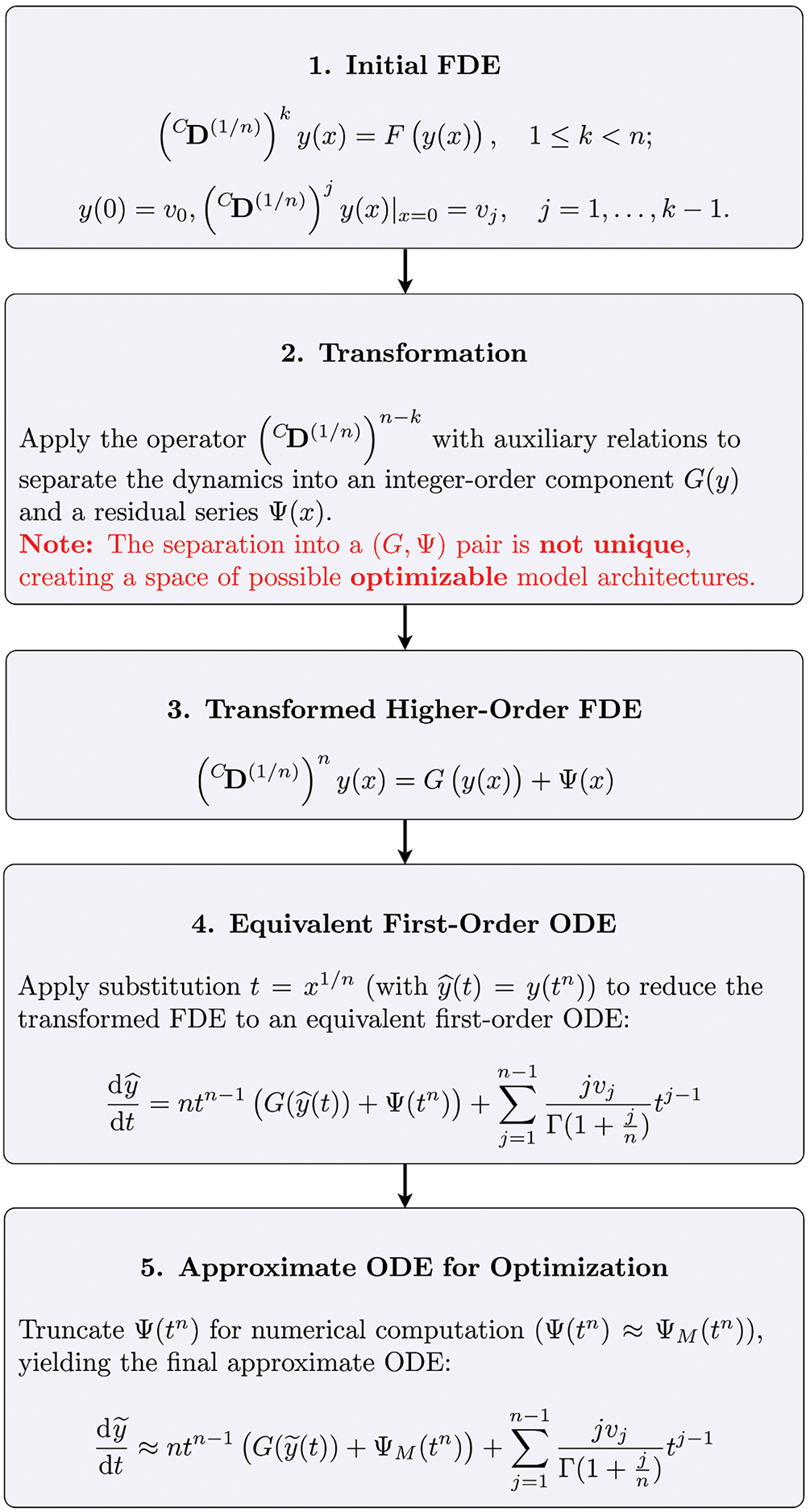
Figure 1: The step-by-step process described in Section 3.2 which is used in obtaining an approximate ODE for a given FDE

3.3 Optimization Framework

To explore the range of possible architectures and find an optimal one, the function G(y) is parameterized as a polynomial of degree NG:

G(y;b)=∑p=0NGbpyp,(24)

where b=(b0,b1,…,bNG) is the vector of coefficients to be optimized. The choice of a polynomial basis for parameterizing G(y) is motivated by several factors. From a theoretical standpoint, the Weierstrass approximation theorem suggests that polynomials can uniformly approximate any continuous function on a closed interval, making them a versatile choice for representing the unknown integer-order dynamics. From a practical standpoint, polynomials offer a straightforward parameterization via their coefficients and are computationally tractable, simplifying both the construction of the approximate ODE and the evaluation of the objective function. While other basis functions, such as rational functions or trigonometric series, could be employed in future extensions of this work, polynomials provide a simple and interpretable starting point for this foundational study, where the resulting low-degree models offer clear insights into the system’s dominant dynamics.

The overall optimization procedure is structured as follows:

1.   Define the search space: For a given polynomial degree NG, the coefficients b define a potential ODE architecture. For any chosen b, the corresponding infinite power series term Ψ(x;b) is implicitly defined by:

Ψ(x;b)=(CD(1/n))ny(x)−G(y(x);b)=∑j=0∞ψj(b)wj(n).(25)

The coefficients ψj(b) of this series depend on the coefficients vj of the FPS solution y(x), which are determined by the original FDE (18), and the chosen parameters b. Specifically, if

(CD(1/n))ny(x)=∑j=0∞vj+nwj(n),(26)

and

G(y;b)=∑j=0∞gj(b)wj(n),(27)

then

ψj(b)=vj+n−gj(b).(28)

2.   Compute quality metrics: The goal is to find a parameter vector b∗ that simultaneously minimizes two often competing objectives: solution accuracy and structural simplicity. This constitutes a multi-objective optimization problem, also known as a Pareto optimization problem. A common and effective method for solving such problems, adopted in this work, is the weighted sum method, which incorporates the multiple objectives into a single target function. The two objectives are defined as follows:

•   The solution accuracy, quantified by the Root Mean Square Error (RMSE) between the approximate solution y(x;b,M) and a high-fidelity reference solution yref(x):

RMSE(b)=1P∑j=1P(y(xj;b,M)−yref(xj))2,(29)

where the error is evaluated over a discrete set of P points, {xj}j=1P, within the solution interval. The reference yref(x) can be an exact solution if known, or a numerical solution computed using established numerical methods.

•   The model’s structural simplicity, quantified by the magnitude of the truncated residual series, measured by its L2-norm, ‖ΨM(b)‖2:

‖ΨM(b)‖2=∫0tmax(ΨM(t;b))2dt,(30)

where tmax=X1/n is the upper limit of the integration interval corresponding to the FDE’s domain [0,X].

3.   Establish a baseline for normalization: To create a balanced optimization problem from these two potentially different-scaled objectives, a dynamic normalization strategy is employed. First, a baseline parameter vector, bbaseline, is defined to be identical to the analytical structure of the original FDE’s forcing function, F(y). The objectives are evaluated once at this baseline to obtain reference values:

RMSEref=RMSE(bbaseline);‖ΨM‖ref=‖ΨM(bbaseline)‖2.(31)

For example, given a linear forcing function of the form F(y)=a0+a1y, the baseline is chosen as bbaseline=[a0,a1,0,…,0], fixing the initial guess for the polynomial G(y) to be identical to F(y). The metrics defined in the previous point are evaluated to obtain reference values, RMSEref and ‖ΨM‖ref.

4.   Define the final objective function: The final, normalized scalar objective function Tnorm(b) to be minimized is a weighted sum of the normalized components:

MinimizebTnorm(b)=κ1RMSE(b)RMSEref+κ2‖ΨM(b)‖2‖ΨM,ref‖2.(32)

In this study, balanced weights κ1=κ2=0.5 are used. Since each term in the objective function is normalized by its respective baseline value, the two components are rendered dimensionless and of a comparable magnitude. This makes equal weighting a natural and unbiased choice, ensuring that the optimization seeks a balanced improvement relative to a consistent, problem-derived baseline without a priori favoring either solution accuracy or structural simplicity.

5.   Perform global optimization: A global optimization algorithm, Particle Swarm Optimization (PSO) [27], is used to find the optimal parameter vector b∗ that minimizes Tnorm(b). PSO algorithm is widely recognized for its strong practical performance in finding high-quality solutions and its effectiveness in navigating complex, non-convex search spaces often found in engineering problems [28]. Its implementation is relatively straightforward and it requires tuning fewer parameters compared to other metaheuristics, making it a robust and practical choice for this foundational work. Note that as a stochastic heuristic, PSO does not mathematically guarantee convergence to the global optimum, and a formal proof of convergence for such methods is a topic of ongoing research beyond the scope of this foundational study. Moreover, given the likely non-convex nature of the optimization landscape defined by the objective function Tnorm(b), the existence of multiple local optima is possible. However, the framework does not aim to prove the existence of a single, unique optimal integer-order structure. Instead, its objective is to identify a parsimonious and high-performing ODE architecture that provides valuable structural insight. The consistency of the results across different parameter spaces, as demonstrated in following Sections, suggests that the method robustly identifies meaningful structures rather than spurious local minima.

While other algorithms like genetic algorithms or simulated annealing could also be applied, a comparative study of different optimizers was considered beyond the scope of this work, which aims to demonstrate the feasibility of the overall framework. It is important to note that the normalized objective function Tnorm(b) serves as a balanced internal metric to guide the optimizer within a specific problem configuration. However, for the purpose of comparing the method’s performance across different FDE configurations (e.g., with different parameters or initial conditions), the final, un-normalized physical metrics—the RMSE and the L2-norm of the truncated residual fractional series—are used as the primary basis for assessment and comparison.

To summarize the procedure presented in section succinctly, see the steps outlined in Fig. 2.

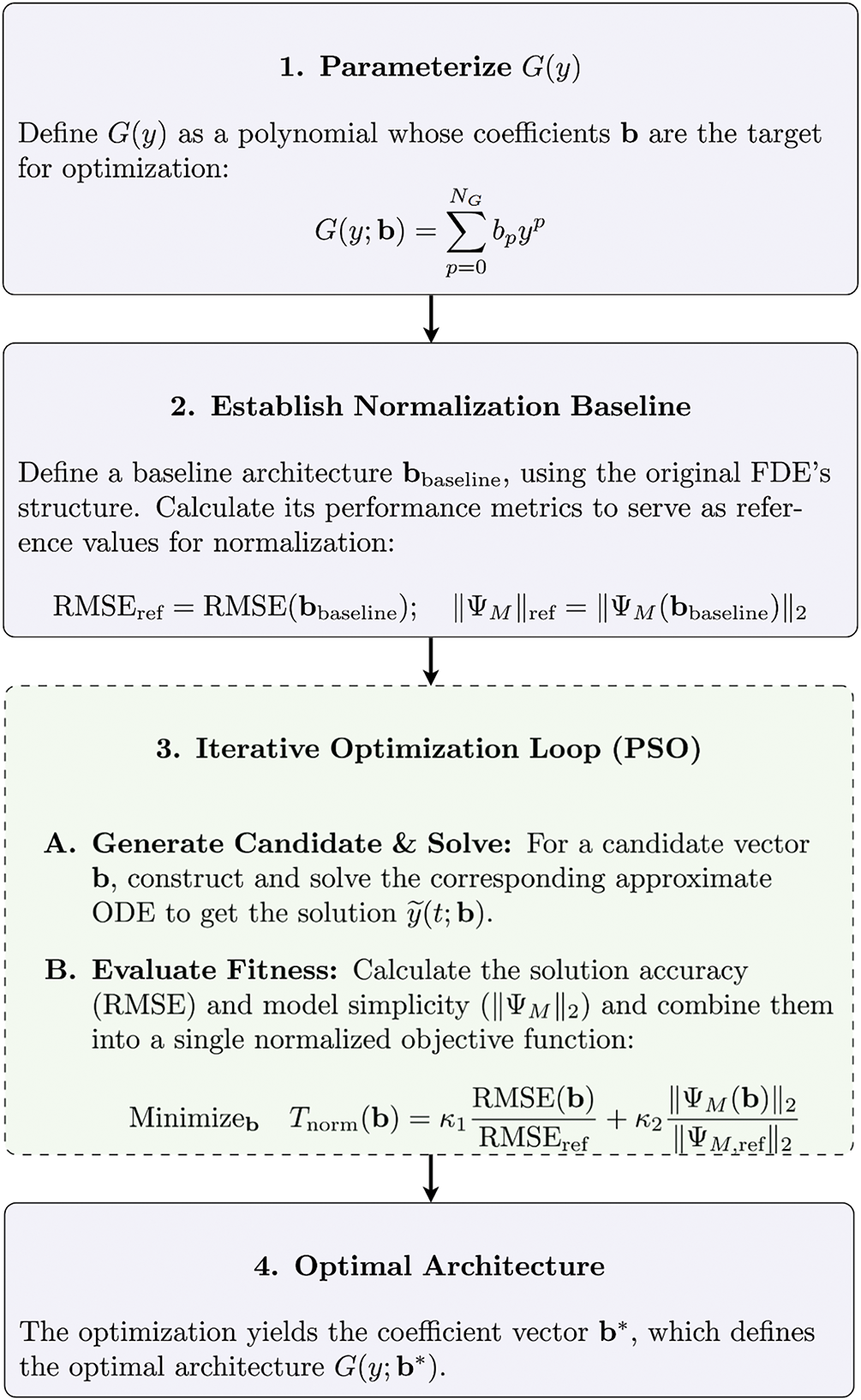
Figure 2: The step-by-step process described in Section 3.3, outlining the procedure for determining optimal b∗ values which define part of the architecture of the FDE

3.4 Computational Complexity

The computational complexity of the proposed framework is primarily determined by the global optimization process, as the initial FDE-to-ODE transformation is performed only once. The dominant source of computational cost is the iterative evaluation of the objective function Tnorm(b) within the PSO algorithm. The total cost can be approximated as the product of the number of PSO particles, the number of iterations, and the cost of a single objective function evaluation.

The complexity of a single evaluation for a candidate parameter vector b is composed of three main parts. First, the approximate ODE is constructed by calculating the coefficients of the truncated residual series ΨM(tn;b). The cost of this step depends on the polynomial degree of the integer-order component NG and the truncation order of the series M. Second, the approximate ODE (23) is solved using a standard numerical integrator, where the cost is dependent on the solver’s efficiency, the required tolerance, and the stiffness of the resulting ODE over the integration interval. Third, the quality metrics are calculated, where the RMSE is computed over P discrete points, resulting in a cost proportional to P, and the L2-norm of the residual series requires a numerical integration.

It is important to contextualize this computational cost. The optimization procedure is a computationally intensive, offline analysis performed once for a given FDE structure. The objective of this one-time investment is not to produce a single numerical solution more efficiently, but rather to obtain a simplified, integer-order ODE architecture that reveals fundamental properties of the FDE’s dynamics. The analytical advantage gained from this process—a deeper insight into the interplay between local and non-local behaviors—is the primary justification for the proposed computational framework.

4  Results

This section presents numerical experiments designed to illustrate the proposed methodology for finding optimal ODE architectures. The approach is applied to two distinct cases: a linear FDE with a known exact solution and a nonlinear (quadratic) FDE where a high-fidelity numerical solution serves as the reference. The primary goal is to demonstrate the optimization process and analyze the resulting ODE structures, particularly the optimized polynomial G(y;b∗) and its relationship to the original FDE dynamics.

4.1 Case 1: Linear FDE

First, a linear FDE, involving the iterated Caputo derivative (CD(1/3))2, corresponding to n=3,k=2 in the general formulation (18), is considered:

(CD(1/3))2y(x)=a0+a1y(x),(33)

subject to initial conditions y(0)=v0 and (CD(1/3)y)(0)=v1.

This FDE possesses an exact analytical solution expressed using the Mittag-Leffler functions [29]:

yref(x)=v0E23,1(a1x23)+v1x13E23,43(a1x23)+a0x23E23,53(a1x23).(34)

This exact solution serves as the high-fidelity reference yref(x) for calculating the RMSE in the optimization process.

The methodology transforms the FDE (33) into the (CD(1/3))3-type FDE

(CD(1/3))3y(x)=G(y(x);b)+Ψ(x;b),(35)

which is then reduced to the approximate ODE (23) using the parameterized polynomial G(y;b)=∑p=0NGbpyp and the truncated term ΨM(tn;b). The optimization seeks the coefficients b∗ for the polynomial G(y;b) that minimize the normalized target function (32). Key parameters used in the experiments are summarized in Table 1.

First, the case

a0=−1.5,a1=0.5,v0=1.5,v1=2(36)

is analyzed. The results, summarized in Table 2, show that the case of NG=2 represents the optimal trade-off in model complexity for this problem configuration. It provides a substantial improvement over the NG=1 model, reducing the normalized target value by over 90% and the un-normalized RMSE by a factor of approximately 50. This demonstrates that a quadratic model for G(y) is more effective at capturing the intrinsic integer-order dynamics of the fractional system.

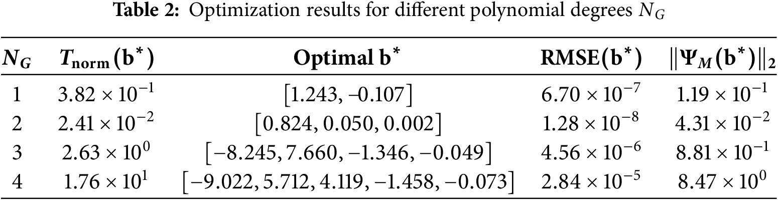
Conversely, increasing the complexity further to NG=3 and NG=4 results in a significant degradation in performance. The final target values for these models are two and three orders of magnitude worse than that of the NG=2 model, respectively, with corresponding increases in both the final RMSE and residual fractional series norm. This indicates that higher-degree polynomials do not yield a better representation for this system. Such a decline in performance suggests that the optimization process either encounters a more challenging, high-dimensional parameter space or the models begin to overfit the reference solution.

Moreover, Fig. 3 provides a visual representation of the optimized residual fractional series, which corroborates the numerical results in Table 2. The plot clearly shows that the residual fractional series for the NG=1 and NG=2 models are well-behaved, remaining close to zero across the entire interval. In stark contrast, the residual series for the higher-complexity models (NG=3 and NG=4) are substantially larger and display significant growth, which is consistent with their much larger L2-norms. This visualization reinforces the conclusion that the quadratic architecture is superior, as it not only minimizes the solution error but also produces the most compact residual fractional series.

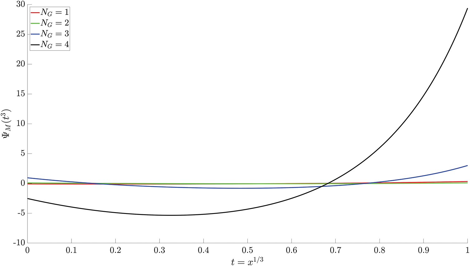
Figure 3: Optimized residual fractional series ΨM(t3) for the linear FDE for polynomial degrees NG=1,2,3, and 4. The plot shows that the quadratic model (NG=2) yields a small and well-behaved residual series. The significant growth of the residuals for higher-degree models (NG≥3) is could be an indicator of overfitting, which corresponds to the poor performance metrics reported in Table 2

These findings are significant, as they demonstrate the framework’s capacity to identify an optimal level of complexity, beyond which adding more parameters is detrimental. The analysis reveals that the underlying integer-order dynamics of this specific fractional system are most effectively represented not by a simple linear model, but by a quadratic one.

4.1.1 Parameter Space Analysis of Optimal Model Complexity

To further investigate the robustness of the optimal model architecture, a parameter space analysis is conducted. The optimization procedure is systematically applied across a grid of FDE coefficients, with a0 and a1 each varying over the range [−1,1]. For each pair of (a0,a1) coefficients, the optimal polynomial degree NG∈{1,2,3,4} is determined by identifying the model that yields the minimum normalized target value, Tnorm. The initial conditions are held constant at v0=1.5 and v1=2, and all other computational parameters are maintained as specified in Table 1. Note that the objective of this analysis is to demonstrate the stability of the optimal architecture across a representative, bounded domain of system parameters, rather than to conduct a computationally exhaustive global exploration. Naturally, a broader analysis of the parameter space would be a valuable direction for future work.

The results of this meta-analysis are summarized in Table 3, which presents a map of the optimal polynomial degree, NG∗, for each (a0,a1) pair. The analysis reveals a consistent pattern: the quadratic model (NG=2) is the optimal choice in 28 out of the 36 cases tested, representing over 77% of the parameter space.

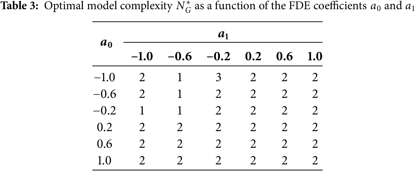
A closer examination of the cases where NG=2 is not the optimal choice provides further insight. In the instances where a linear model (NG=1) is selected, a trade-off between solution accuracy and the magnitude of the residual series is typically observed. For example, for the configuration (a0,a1)=(−0.2,−1.0), the optimal NG=1 model produced a smaller residual series norm (‖ΨM‖2=6.55×10−1) compared to the NG=2 model (‖ΨM‖2=6.92×10−1). Conversely, the NG=2 model achieved a slightly lower RMSE (4.15×10−6) than the NG=1 model (4.86×10−6). This indicates that even in regions where the simpler linear model is marginally preferred by the normalized target function, the quadratic model remains a highly competitive alternative.

The single instance where NG=3 is optimal, at (a0,a1)=(−1.0,−0.2), also warrants comment. For this configuration, the final metrics for the NG=3 model (RMSE = 6.353×10−9, ‖ΨM‖2=5.229×10−2) are nearly identical to those of the NG=2 model (RMSE = 6.356×10−9, ‖ΨM‖2=5.229×10−2), confirming that the performance difference is negligible.

Collectively, these findings strongly support the conclusion that a quadratic ODE architecture provides a robust and broadly applicable representation for the linear fractional differential equation under study. The stability of this result across a wide range of system parameters suggests that the method is not merely finding isolated numerical artifacts but is successfully identifying a fundamental, underlying integer-order structure inherent to the fractional system.

To better understand the structure of the quadratic architecture (NG=2), we now examine how its optimal coefficients b∗=(b0,b1,b2) depend on the original FDE parameters. Fig. 4 visualizes this relationship across the same intervals for a0 and a1 as given in Table 3. Even though the discretization is coarse, it can be seen that the values of b0,b1,b2 do not oscillate wildly and depend smoothly on a0 and a1.

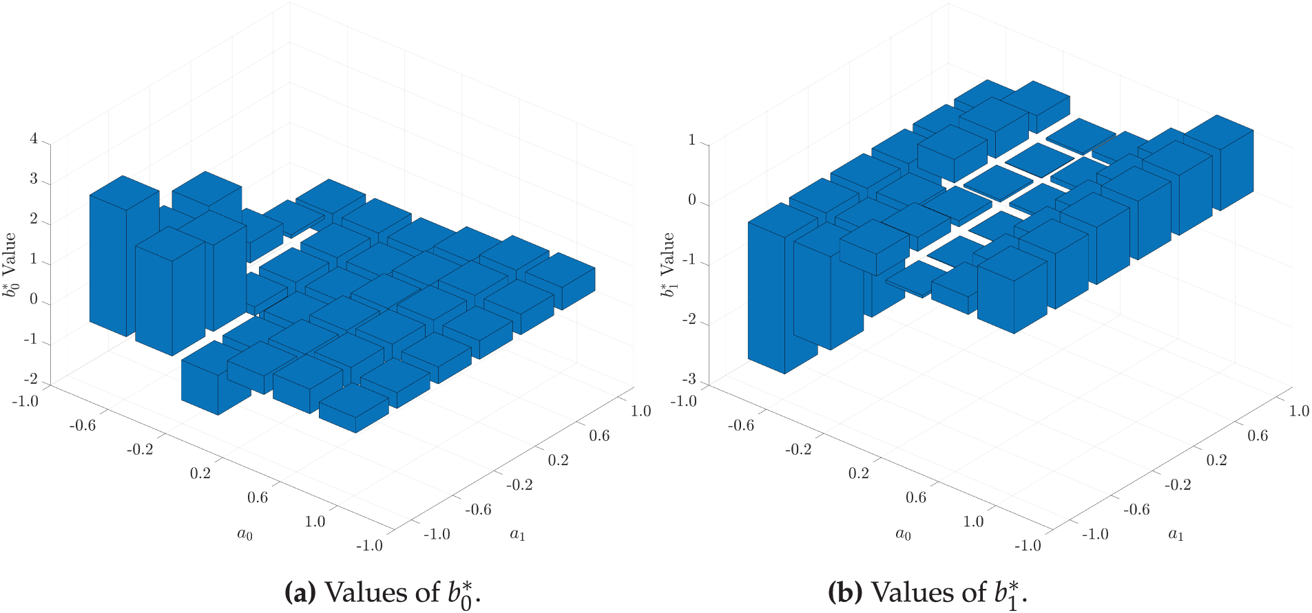
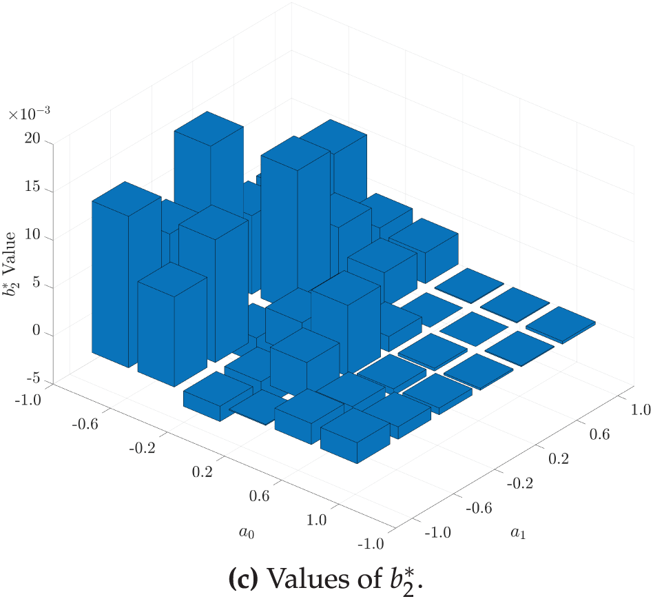
Figure 4: The optimal coefficients b∗=(b0∗,b1∗,b2∗) for the quadratic (NG=2) architecture as the FDE coefficients a0,a1 vary in the interval [−1,1]. It can be seen that the optimal coefficients act as smooth, continuous functions of the FDE parameters, confirming the stability of the identified integer-order structure

4.1.2 Effects of Initial Condition on the Complexity of the Model

To assess whether the optimal ODE architecture is an intrinsic property of the FDE or is dependent on the specific solution trajectory, a second meta-analysis has been performed. In this set of experiments, the FDE coefficients are held constant at a0=−1.5 and a1=0.5, while the initial conditions v0=y(0) and v1=(CD(1/3)y)(0) are varied over the range [−2,2]. All other computational parameters are maintained as specified in Table 1. The same optimization and dynamic normalization procedure is applied to find the optimal polynomial degree NG∗ for each pair of initial conditions.

The results, presented in Table 4, demonstrate a high degree of stability in the optimal model architecture. Across the 36 different initial conditions tested, the quadratic model (NG=2) is identified as the optimal choice in 33 cases, representing approximately 92% of the tested space. This consistency suggests that the optimal ODE representation is largely independent of the specific solution trajectory and is instead determined by the inherent structure of the FDE itself.

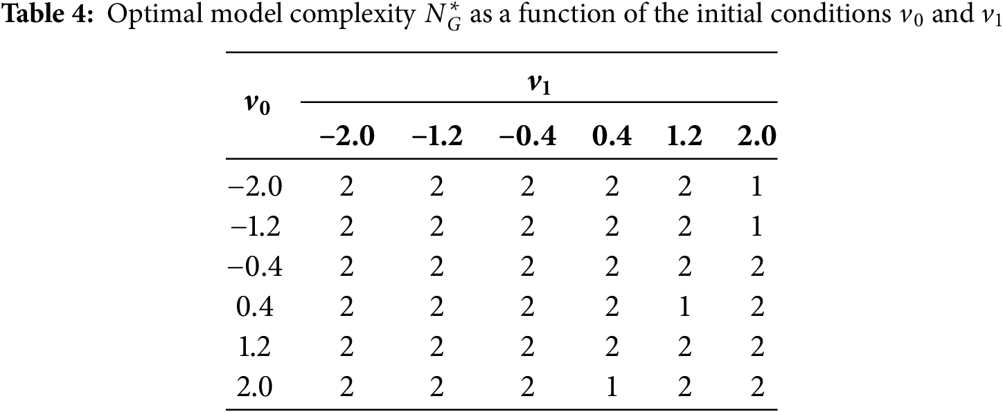
Notably, the few instances where NG=1 has been selected as optimal occurred at or close to the boundaries of the tested parameter space. In these cases, the linear model is found to be genuinely superior across both performance metrics. For example, for the initial conditions (v0,v1)=(−2.0,2.0), the winning NG=1 model produces both a lower RMSE and a smaller residual series norm than the NG=2 model. However, the overwhelming dominance of the quadratic model across the vast majority of the parameter space remains the principal finding. Furthermore, the higher-complexity models (NG=3 and NG=4) consistently underperform, often yielding results that are orders of magnitude worse than the simpler models.

The combined results from the parameter space analyses of both the FDE coefficients and the initial conditions provide strong evidence for the central hypothesis. The methodology consistently identifies a quadratic ODE as the most suitable integer-order representation for the given linear FDE. This stability across different system parameters and solution trajectories indicates that the optimization framework is successfully uncovering a fundamental, intrinsic property of the fractional system’s dynamics, rather than artifacts of a specific configuration.

4.1.3 Sensitivity Analysis on the Truncation Order of the Residual of the Fractional Series

A sensitivity analysis has been conducted to evaluate the influence of the residual fractional series truncation order, M, on the performance of the optimization framework. For this study, the FDE coefficients and initial conditions are held constant at the values used in the first example (a0=−1.5,a1=0.5,v0=1.5,v1=2), while the parameter M is varied from 5 to 20. All other computational parameters are maintained as specified in Table 1. The primary objective is to determine if the choice of the optimal model complexity, NG∗, is stable with respect to the accuracy of the residual fractional series approximation.

The results, summarized in Table 5, reveal a distinct trend. For lower values of M (specifically, M≤7), the optimization procedure has selected a cubic polynomial (NG=3) as the optimal architecture. However, as M increases to 8 and beyond, the optimal model complexity consistently stabilizes at the quadratic model (NG=2).

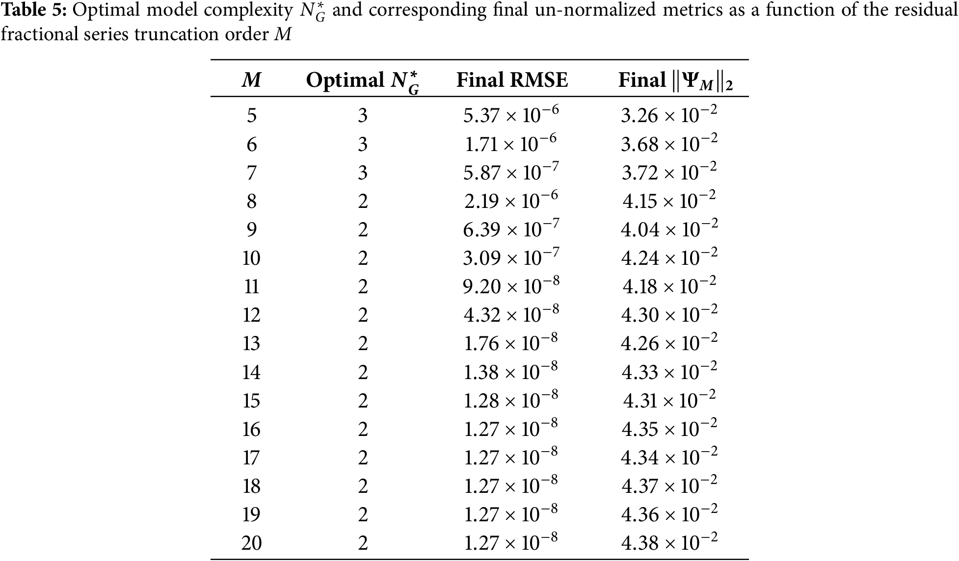
This transition in the optimal model complexity is a significant finding. It suggests that when the residual fractional series ΨM(tn) is poorly approximated (i.e., when M is small), the optimization framework compensates by selecting a more complex polynomial G(y) to capture the dynamics that are missing from the truncated series. As the series approximation becomes more accurate with increasing M, this compensation is no longer necessary, and the framework is able to identify the underlying quadratic structure of the system.

Furthermore, an examination of the final un-normalized metrics reveals the practical limits of increasing the residual series order. While the final RMSE of the optimal solution improves substantially as M increases from 8 to 15, it converges to approximately 1.27×10−8 for M≥15. Similarly, the final residual series norm, ‖ΨM‖2, stabilizes around a value of 4.3×10−2. This indicates that beyond a certain point (M≈15 for this problem), further increasing the number of terms in the residual fractional series approximation yields no discernible improvement in the quality of the final solution.

In conclusion, this sensitivity analysis demonstrates the robustness of the proposed methodology. It shows that provided the residual fractional series is approximated with a sufficient number of terms, the optimization consistently converges to the same optimal ODE architecture. This reinforces the conclusion that the framework is successfully identifying an intrinsic and stable integer-order representation of the fractional system.

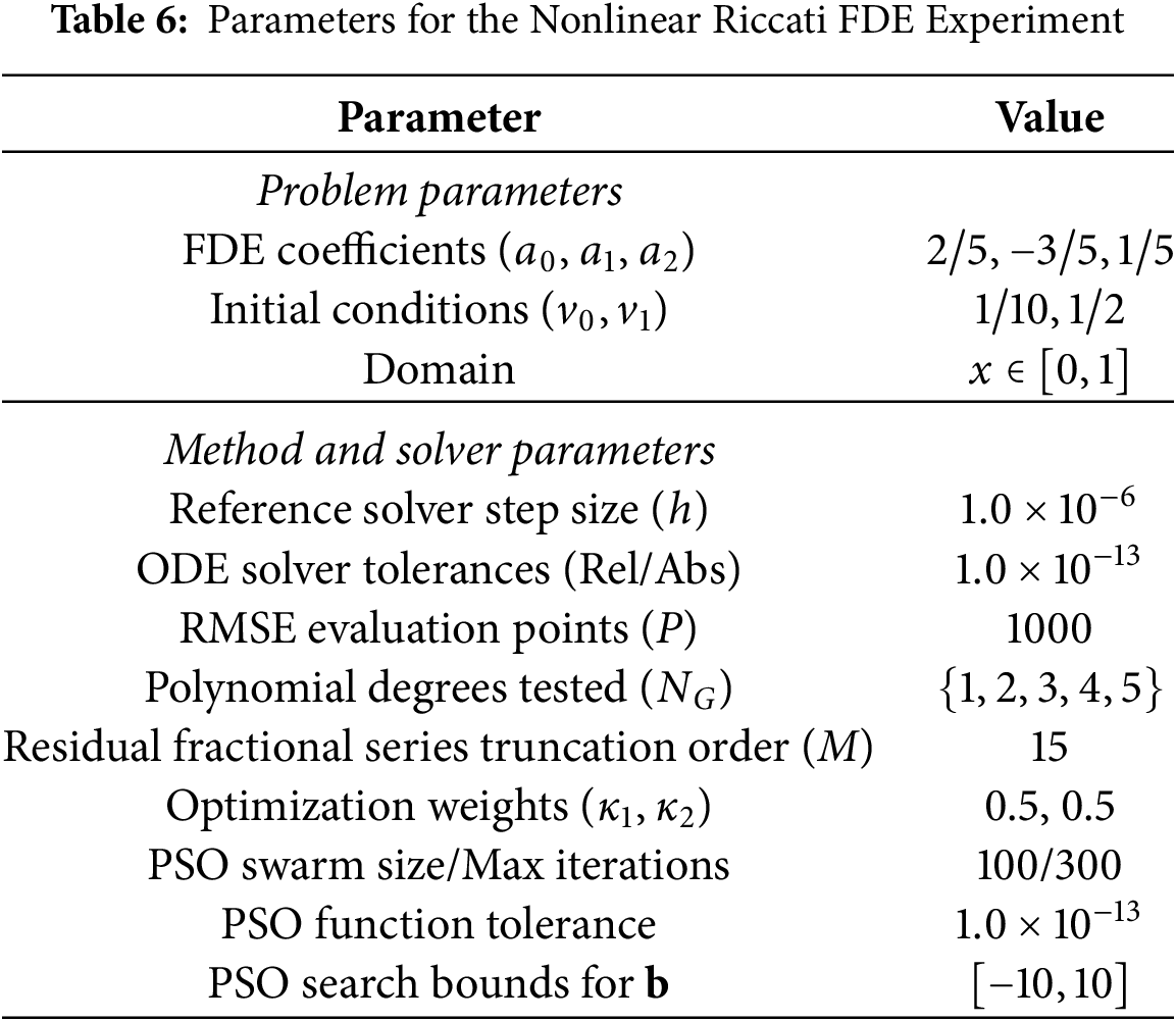
4.2 Case 2: Nonlinear Riccati FDE

To demonstrate the methodology’s applicability to nonlinear problems without known analytical solutions, the framework is applied to a fractional Riccati FDE. The equation, corresponding to n=3,k=2 in the general formulation, is given by:

(CD(1/3))2y(x)=a0+a1y(x)+a2y(x)2,(37)

subject to initial conditions y(0)=v0 and (CD(1/3)y)(0)=v1. An exact analytical solution for (37) is not known. Therefore, a high-fidelity numerical solution obtained using Garrappa’s method [30] serves as the reference solution yref(x) for the RMSE calculation during the optimization.

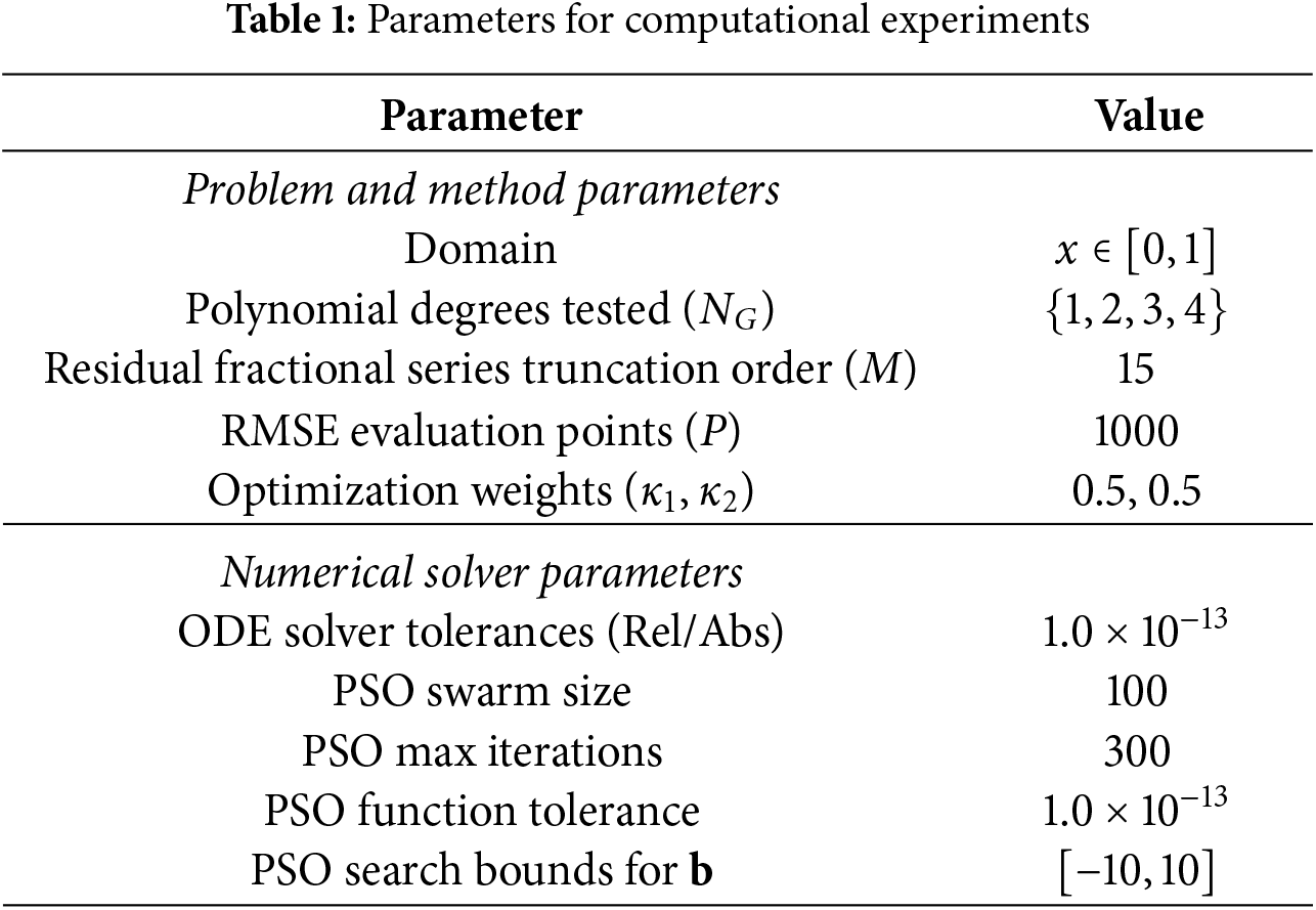
The same optimization framework as in the linear case is used. The specific FDE parameters and computational settings for this experiment are detailed in Table 6.

The optimization results for polynomial degrees NG from 1 to 5 are presented in Table 7 and Fig. 5. The analysis reveals a different pattern of results compared to the linear FDE. In this case, the optimization identifies the cubic model (NG=3) as the optimal architecture, achieving the lowest target value of 3.43×10−2. This optimal result is driven by the model’s exceptional solution accuracy; its final RMSE of 1.27×10−8 is more than two orders of magnitude lower than that of the next best competitor, the NG=2 model.

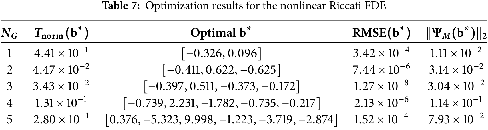
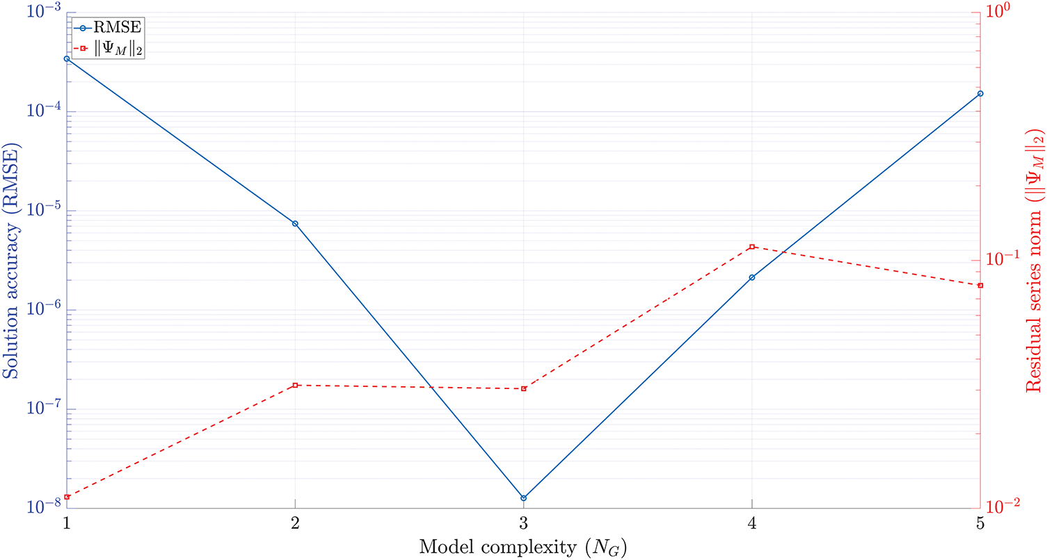
Figure 5: The complexity-accuracy trade-off curve for the nonlinear Riccati FDE. The plot shows the final solution accuracy (RMSE, left axis) and the norm of the residual series (‖ΨM‖2, right axis) as a function of the model complexity (NG). The optimal performance is achieved at NG=3

The emergence of an optimal architecture that is of a higher polynomial degree than the original FDE’s nonlinearity is a significant finding. This suggests that the transformation from the FDE to the ODE, which involves the action of a fractional operator on the nonlinear term, generates a richer set of dynamics. The optimization framework discovers that it is more effective to capture the dominant part of these emergent dynamics within the integer-order component G(y) using a cubic term, rather than relegating them to the residual series Ψ(x). This choice results in a model that achieves a substantially lower solution error, providing insight into the complex interplay between the fractional operator and the system’s inherent nonlinearity.

A trade-off between solution accuracy and the magnitude of the residual fractional series is also observed. While the linear model (NG=1) produced the smallest residual fractional series, its significantly higher RMSE resulted in a much poorer overall target value. This illustrates a case where the optimizer correctly favored the model with superior accuracy, even at the cost of a marginally larger residual series. The optimized residual fractional series are plotted in Fig. 6. The visualization confirms that the residual series for the NG=1 model has the smallest overall magnitude, consistent with its minimal L2-norm, while the residual series for the more accurate NG=2 and NG=3 models are similarly well-behaved and small in magnitude. In contrast, the residual series for NG=4 and NG=5 are significantly larger and more oscillatory, providing a visual explanation for their poor performance.

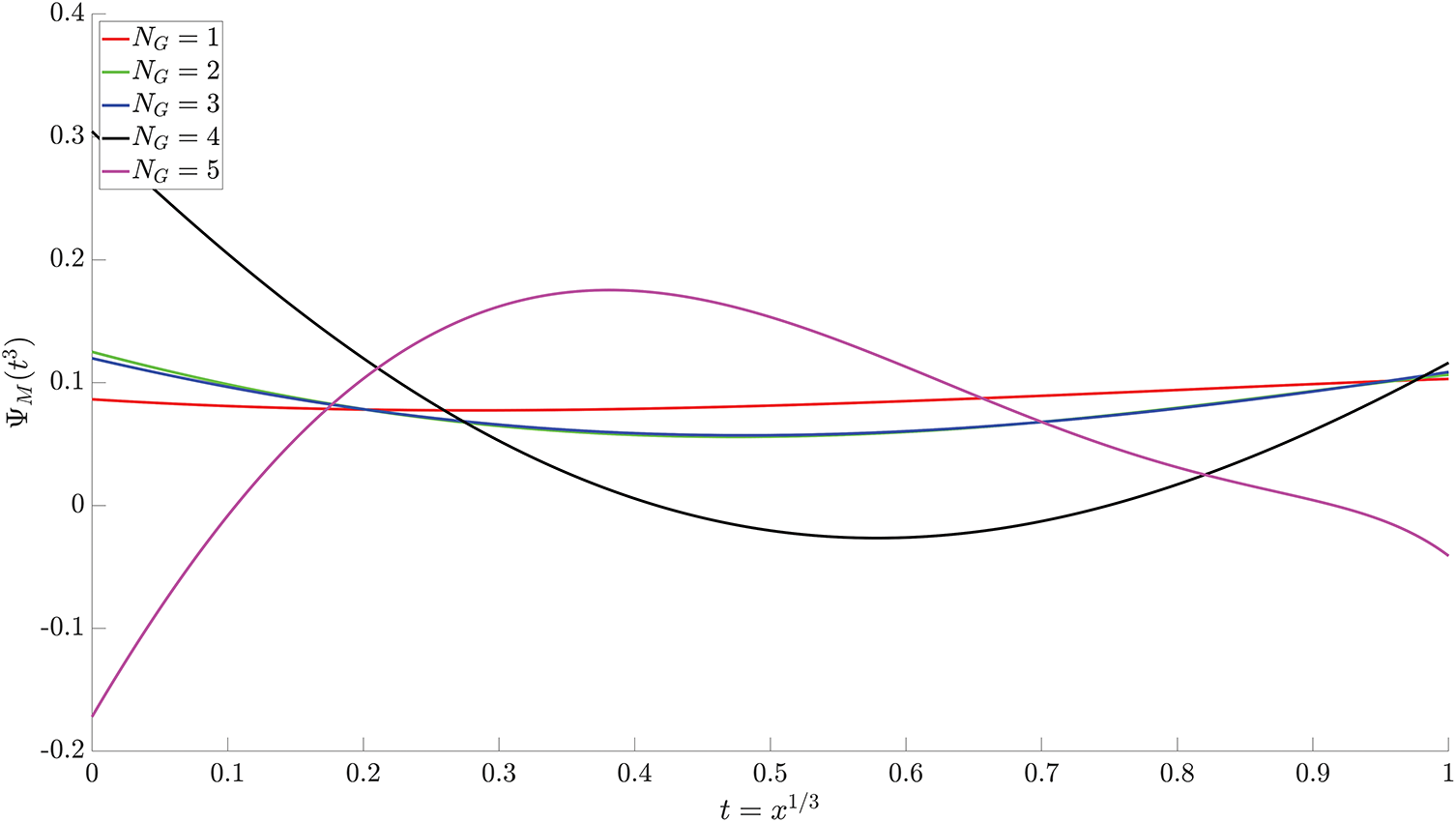
Figure 6: Optimized residual fractional series ΨM(t3) for the Riccati FDE for polynomial degrees NG=1,…,5. The visualization confirms that while the NG=1 model yields the smallest residual, the optimal NG=3 model remains well-behaved. The large and oscillatory residuals for the higher-degree models (NG≥4) provide a visual explanation for their suboptimal performance

Consistent with the findings from the linear analysis, increasing the model complexity beyond an optimal point (NG>3) is detrimental. This result reinforces the conclusion that the methodology is capable of identifying an optimal level of complexity for the approximating ODE, which is sensitive to the underlying structure of the FDE. The primary significance of this experiment is the demonstration that the framework is not limited to linear FDEs, but serves as a versatile tool for the structural analysis of a broader class of fractional differential equations.

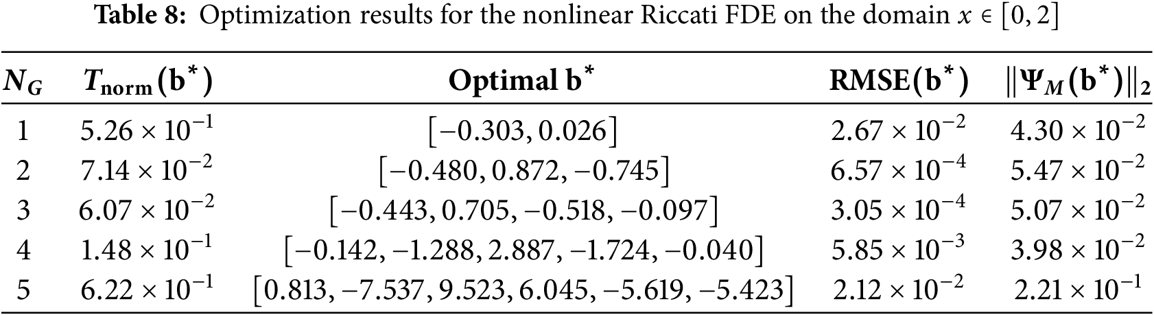
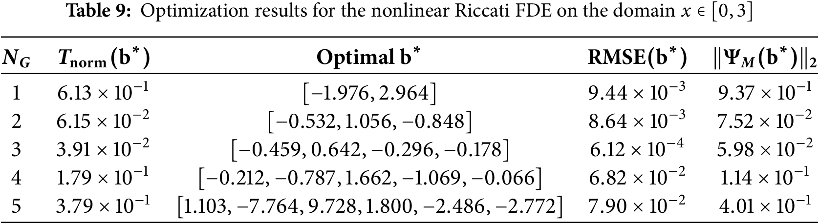
4.2.1 Effect of the Integration Horizon

To verify the effectiveness and generality of the proposed framework over different integration intervals, the experiment on the nonlinear Riccati FDE was repeated for two longer domains: x∈[0,2] and x∈[0,3]. The objective of this analysis is to determine if the optimal model architecture identified in the previous section is a robust structural property of the FDE or an artifact of the specific integration horizon. All FDE and computational parameters are kept identical to those in Table 6, with only the domain of the problem being extended. The reference solution for the RMSE calculation on the extended domains was again obtained using Garrappa’s method.

The optimization results for the extended domains are presented in Tables 8 and 9. The analysis reveals a consistency in the optimal architecture. For both the x∈[0,2] and x∈[0,3] intervals, the cubic model (NG=3) is unambiguously identified as the superior choice, achieving the lowest normalized target value in each case. While the absolute RMSE values naturally increase as the integration interval becomes longer, the optimizer’s structural preference remains stable. This finding strongly supports the conclusion that the identified cubic architecture is not a feature of a specific problem configuration but rather an intrinsic property of the underlying dynamics of the fractional Riccati equation.

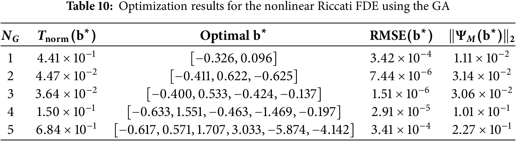
4.2.2 Comparison with an Alternative Optimization Algorithm

To ensure that the findings of this study are not specific to the choice of the optimization algorithm, the experiment on the nonlinear Riccati FDE presented at the beginning of this section (with the integration interval x∈[0,1]) was repeated using an alternative global optimizer. The Genetic Algorithm (GA), which is another well-established, population-based metaheuristic, was chosen for this comparative analysis. The GA was configured with parameters comparable to those used for the PSO; specifically, the population size was set to 100 and the maximum number of generations to 300, mirroring the swarm size and maximum iterations of the PSO, respectively. All other FDE and method parameters were kept identical to those listed in Table 6.

The optimization results obtained using the GA are presented in Table 10 and are consistent with the PSO results from Table 7. GA also unambiguously identifies the cubic model (NG=3) as the optimal architecture, achieving the lowest normalized target value. While the final numerical metrics differ slightly between the two algorithms, which is a common occurrence given their stochastic nature, the central conclusion remains the same. This successful replication of the result with a different optimizer provides strong evidence that the identified cubic architecture is a genuine feature of the FDE’s underlying dynamics and not an artifact of the optimization method used to find it.

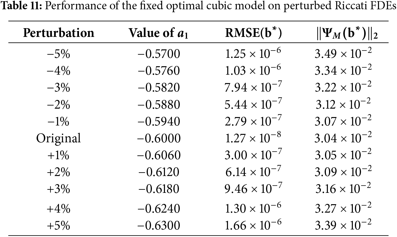
4.2.3 Sensitivity Analysis of the Optimal Solution

To assess the robustness of the optimization outcomes, a sensitivity analysis was performed on the optimal solution found by the PSO algorithm for the nonlinear Riccati FDE (see Table 7). The objective of this analysis is to determine if the identified optimal architecture is stable with respect to small variations in the FDE’s parameters. For this study, the optimal cubic architecture (NG=3) and its corresponding coefficient vector b∗ were held fixed. The performance of this fixed model was then evaluated on a set of perturbed FDEs, where the coefficient a1 was varied in increments of 1% over the range of ±5% from its original value. For each perturbed FDE, a new high-fidelity reference solution was computed to ensure an accurate RMSE calculation.

The results of this analysis are presented in Table 11. The results show that the optimal solution exhibits structural stability, with performance metrics degrading continuously with respect to parameter perturbations. Both the final RMSE and the norm of the residual series are minimized for the unperturbed, original problem and increase monotonously and symmetrically as the perturbation magnitude grows. This demonstrates that the optimal solution represents a stable optimum within a local neighborhood of the parameter space, confirming the robustness of the optimization outcome.

5  Discussion

The effectiveness of the presented approach was demonstrated on both a linear FDE and a nonlinear fractional Riccati equation. These cases were selected as representative examples to establish the feasibility of the proposed structural analysis on both a linear problem with a known analytical solution and a nonlinear problem requiring a numerical reference solution. The fractional Riccati equation, in particular, serves as a relevant nonlinear model due to its importance in applied mathematics for modeling real-world phenomena, including population dynamics and tumor growth [31], where the inclusion of memory effects via fractional operators is an active area of research to improve model realism [32]. The numerical results consistently show that the method can identify an optimal, low-degree polynomial ODE that accurately captures the dynamics of the fractional system. For the linear FDE, a quadratic architecture has been found to be robustly optimal across a wide range of system parameters and initial conditions, revealing an underlying structure more complex than the original linear forcing term. For the nonlinear Riccati FDE, a cubic architecture has been identified as optimal.

Notably, the results often indicate a significant decline in performance when the model complexity is increased beyond the optimal degree which could indicate the model’s sensitivity to over-parameterization. The primary goal of this work is to introduce the novel concept of structural optimization for FDEs and demonstrate its feasibility on representative examples. Thus, in this foundational study, objective function is designed to measure only the core metrics of interest: solution accuracy and the magnitude of the residual series. It does not contain an explicit regularization term that would penalize model complexity. However, while the framework minimizes the error against the reference, the dual nature of the objective function, which also penalizes ‖ΨM(b)‖2, acts as an implicit regularizer promoting structural simplicity. Thus, while the absence of explicit regularization can make the optimization landscape for over-parameterized models more challenging, this sensitivity is advantageous for model identification. The resulting performance decline acts as a clear and unambiguous signal against overfitting, effectively confirming that the identified low-degree architecture is not merely a good approximation, but the most robust representation of the system’s underlying integer-order dynamics. This paves the way for future research. A natural extension of this work would be to incorporate regularization techniques into the framework. Doing so would likely stabilize the optimization for higher-degree polynomials by promoting sparse solutions, potentially transforming the proposed tool into an even more powerful predictive one.

A crucial distinction must be drawn between the proposed framework and other established methodologies. While high-fidelity numerical methods provide accurate solutions, they yield a numerical result without offering deeper insight into the underlying structure of the FDE. It is not the goal of this study to compete with these methods in terms of raw numerical precision, but to introduce a novel tool for structural analysis. By identifying an optimal, low-degree integer-order ODE, our framework provides a simplified yet powerful lens through which to understand the intrinsic dynamics of the fractional system. It emphasizes the interplay between local, integer-order behavior (captured by G(y)) and non-local, memory-dependent effects (captured by Ψ(x)). Moreover, it addresses a forward problem of equation analysis, which is fundamentally different from the inverse problem solved by data-driven discovery methods like SINDy, where the governing equation itself is the unknown to be found from data. This structural understanding provided by the proposed method is a valuable analytical complement to purely numerical solutions, offering a new perspective on the fundamental properties of fractional systems.

6  Conclusion

This paper introduces a novel computational framework for identifying optimal integer-order ODE representations for FDEs containing iterated Caputo derivatives. The methodology utilizes a transformation that recasts the FDE into a higher-order form composed of an integer-order dynamic component G(y) and a residual fractional power series Ψ(x). By parameterizing G(y) as a polynomial and employing a global optimization algorithm, the framework seeks an architecture that simultaneously minimizes the solution error and the magnitude of the residual series. Presented findings underscore the framework’s ability to discern an appropriate level of complexity and avoid overfitting, thereby providing genuine insight into the system’s intrinsic integer-order dynamics.

In summary, this work provides a new tool for analyzing the underlying structure of FDEs and gaining deeper insights into the interplay between local and non-local dynamics. The primary limitations of this foundational study are its focus on a specific class of FDEs with iterated Caputo derivatives and the use of a polynomial basis for parameterization, which may not be optimal for all systems.

Future research could extend this framework to broader classes of FDEs, including its scalability to high-dimensional and coupled systems of equations or those involving other fractional operators (such as the Atangana-Baleanu or Riemann-Liouville operators, etc.). Furthermore, exploring alternative parameterizations for the integer-order component, such as rational functions, may reveal even richer structural properties of fractional systems.

Acknowledgement: This research was funded by the Research Council of Lithuania.

Funding Statement: This project has received funding from the Research Council of Lithuania (LMTLT), agreement No. S-PD-24-120.

Author Contributions: The authors confirm contribution to the paper as follows: Conceptualization, Tadas Telksnys, Inga Telksniene, Minvydas Ragulskis and Raimondas Čiegis; methodology, Tadas Telksnys, Inga Telksniene, Minvydas Ragulskis and Romas Marcinkevičius; software, Inga Telksniene and Romas Marcinkevičius; validation, Inga Telksniene, Tadas Telksnys and Romas Marcinkevičius; formal analysis, Minvydas Ragulskis, Zenonas Navickas, Tadas Telksnys, Inga Telksniene and Raimondas Čiegis; investigation, Inga Telksniene, Tadas Telksnys, Romas Marcinkevičius, Zenonas Navickas, Minvydas Ragulskis and Raimondas Čiegis; writing—original draft preparation, Inga Telksniene, Tadas Telksnys and Minvydas Ragulskis; writing—review and editing, Inga Telksniene, Tadas Telksnys, Romas Marcinkevičius, Zenonas Navickas, Minvydas Ragulskis and Raimondas Čiegis; supervision, Minvydas Ragulskis and Raimondas Čiegis; funding acquisition, Inga Telksniene and Raimondas Čiegis. All authors reviewed the results and approved the final version of the manuscript.

Availability of Data and Materials: Not applicable.

Ethics Approval: Not applicable.

Conflicts of Interest: The authors declare no conflicts of interest to report regarding the present study.

Abbreviations

References

1. Podlubny I. Fractional differential equations: an introduction to fractional derivatives, fractional differential equations, to methods of their solution and some of their applications. San Diego, CA, USA: Academic Press; 1999. [Google Scholar]

2. Suzuki JL, Kharazmi E, Varghaei P, Naghibolhosseini M, Zayernouri M. Anomalous nonlinear dynamics behavior of fractional viscoelastic beams. J Comput Nonlinear Dyn. 2021;16(11):111005. doi:10.1115/1.4052286. [Google Scholar] [PubMed] [CrossRef]

3. Loghman E, Bakhtiari-Nejad F, Kamali A, Abbaszadeh M, Amabili M. Nonlinear vibration of fractional viscoelastic micro-beams. Int J Non Linear Mech. 2021;137(1–4):103811. doi:10.1016/j.ijnonlinmec.2021.103811. [Google Scholar] [CrossRef]

4. Ali I, Khan SU. A dynamic competition analysis of stochastic fractional differential equation arising in finance via pseudospectral method. Mathematics. 2023;11(6):1328. doi:10.3390/math11061328. [Google Scholar] [CrossRef]

5. Li B, Zhang T, Zhang C. Investigation of financial bubble mathematical model under fractal-fractional Caputo derivative. Fractals. 2023;31(05):2350050. doi:10.1142/s0218348x23500500. [Google Scholar] [CrossRef]

6. Abdeljawad T, Sher M, Shah K, Sarwar M, Amacha I, Alqudah M, et al. Analysis of a class of fractal hybrid fractional differential equation with application to a biological model. Sci Rep. 2024;14(1):18937. doi:10.1038/s41598-024-67158-8. [Google Scholar] [PubMed] [CrossRef]

7. Singh J, Ganbari B, Kumar D, Baleanu D. Analysis of fractional model of guava for biological pest control with memory effect. J Adv Res. 2021;32(1):99–108. doi:10.1016/j.jare.2020.12.004. [Google Scholar] [PubMed] [CrossRef]

8. Chatterjee AN, Ahmad B. A fractional-order differential equation model of COVID-19 infection of epithelial cells. Chaos Solitons Fract. 2021;147:110952. [Google Scholar]

9. Srivastava H, Jan R, Jan A, Deebani W, Shutaywi M. Fractional-calculus analysis of the transmission dynamics of the dengue infection. Chaos. 2021;31(5):053130. doi:10.1063/5.0050452. [Google Scholar] [PubMed] [CrossRef]

10. Baleanu D, Sajjadi SS, Jajarmi A, Defterli Ö. On a nonlinear dynamical system with both chaotic and nonchaotic behaviors: a new fractional analysis and control. Adv Differ Equ. 2021;2021(1):234. doi:10.1186/s13662-021-03393-x. [Google Scholar] [CrossRef]

11. Jajarmi A, Baleanu D. On the fractional optimal control problems with a general derivative operator. Asian J Control. 2021;23(2):1062–71. doi:10.1002/asjc.2282. [Google Scholar] [CrossRef]

12. Zhang X, Ding F. Optimal adaptive filtering algorithm by using the fractional-order derivative. IEEE Signal Process Lett. 2021;29(1):399–403. doi:10.1109/lsp.2021.3136504. [Google Scholar] [CrossRef]

13. Jackson J, Perumal R. A robust image encryption technique based on an improved fractional order chaotic map. Nonlinear Dyn. 2025;113(7):7277–96. doi:10.1007/s11071-024-10480-7. [Google Scholar] [CrossRef]

14. Ebaid A, Cattani C, Al Juhani AS, El-Zahar ER. A novel exact solution for the fractional Ambartsumian equation. Adv Differ Equ. 2021;2021(1):88. doi:10.1186/s13662-021-03235-w. [Google Scholar] [CrossRef]

15. Sene N. Analytical solutions of a class of fluids models with the Caputo fractional derivative. Fractal Fract. 2022;6(1):35. doi:10.3390/fractalfract6010035. [Google Scholar] [CrossRef]

16. Zabidi NA, Majid ZA, Kilicman A, Ibrahim ZB. Numerical solution of fractional differential equations with Caputo derivative by using numerical fractional predict-correct technique. Adv Cont Disc Mod. 2022;2022(1):26. doi:10.1186/s13662-022-03697-6. [Google Scholar] [CrossRef]

17. Dimitrov Y, Georgiev S, Todorov V. Approximation of Caputo fractional derivative and numerical solutions of fractional differential equations. Fractal Fract. 2023;7(10):750. doi:10.3390/fractalfract7100750. [Google Scholar] [CrossRef]

18. Ali I, Rasheed A, Anwar MS, Irfan M, Hussain Z. Fractional calculus approach for the phase dynamics of Josephson junction. Chaos Solitons Fract. 2021;143:110572. [Google Scholar]

19. Khan M, Rasheed A, Anwar MS. Numerical analysis of nonlinear time-fractional fluid models for simulating heat transport processes in porous medium. ZAMM-J Appl Math Mech/Zeitschrift Für Angewandte Mathematik Und Mechanik. 2023;103(9):e202200544. doi:10.1002/zamm.202200544. [Google Scholar] [CrossRef]

20. Alsulami M, Alyami M, Al-Mazmumy M, Alsulami A. Semi-analytical investigation for the ψ-Caputo fractional relaxation-oscillation equation using the decomposition method. Eur J Pure Appl Math. 2024;17(3):2311–98. [Google Scholar]

21. Iqbal N, Chughtai MT, Ullah R. Fractional study of the non-linear Burgers’ equations via a semi-analytical technique. Fractal Fract. 2023;7(2):103. doi:10.3390/fractalfract7020103. [Google Scholar] [CrossRef]

22. Jin B, Zhou Z. An analysis of Galerkin proper orthogonal decomposition for subdiffusion. ESAIM Math Model Numer Anal. 2017;51(1):89–113. doi:10.1051/m2an/2016017. [Google Scholar] [CrossRef]

23. Khristenko U, Wohlmuth B. Solving time-fractional differential equations via rational approximation. IMA J Numer Anal. 2023;43(3):1263–90. doi:10.1093/imanum/drac022. [Google Scholar] [CrossRef]

24. Brunton SL, Proctor JL, Kutz JN. Discovering governing equations from data by sparse identification of nonlinear dynamical systems. Proc Nat Acad Sci. 2016;113(15):3932–7. doi:10.1073/pnas.1517384113. [Google Scholar] [PubMed] [CrossRef]

25. Navickas Z, Telksnys T, Telksniene I, Marcinkevicius R, Ragulskis M. The fractal structure of analytical solutions to fractional Riccati equation. Fractals. 2024;32(04):2340130. doi:10.1142/s0218348x23401308. [Google Scholar] [CrossRef]

26. Marcinkevicius R, Telksniene I, Telksnys T, Navickas Z, Ragulskis M. The construction of solutions to D(1/n)C type FDEs via reduction to (D(1/n)C)n type FDEs. AIMS Math. 2022;7(9):16536–54. doi:10.3934/math.2022905. [Google Scholar] [CrossRef]

27. Kennedy J, Eberhart R. Particle swarm optimization. In: Proceedings of ICNN’95-International Conference on Neural Networks; 1995 Nov 27–Dec 1; Perth, WA, Australia. p. 1942–8. [Google Scholar]

28. Wang D, Tan D, Liu L. Particle swarm optimization algorithm: an overview. Soft Comput. 2018;22(2):387–408. doi:10.1007/s00500-016-2474-6. [Google Scholar] [CrossRef]

29. Duan J. A generalization of the Mittag–Leffler function and solution of system of fractional differential equations. Adv Differ Equ. 2018;2018(1):239. doi:10.1186/s13662-018-1693-9. [Google Scholar] [CrossRef]

30. Garrappa R. Numerical solution of fractional differential equations: a survey and a software tutorial. Mathematics. 2018;6(2):16. doi:10.3390/math6020016. [Google Scholar] [CrossRef]

31. Timofejeva I, Telksnys T, Navickas Z, Marcinkevicius R, Mickevicius R, Ragulskis M. Solitary solutions to a metastasis model represented by two systems of coupled Riccati equations. J King Saud Univ-Sci. 2023;35(5):102682. doi:10.1016/j.jksus.2023.102682. [Google Scholar] [CrossRef]

32. Arshad S, Baleanu D, Tang Y. Fractional differential equations with bio-medical applications. In: Applications in engineering, life and social sciences, part A. Berlin, Boston: De Gruyter; 2019. p. 1–20. doi:10.1515/9783110571905-001. [Google Scholar] [CrossRef]