Robustness and Performance Comparison of Generative AI Time Series Anomaly Detection under Noise

1  Introduction

Time series anomaly detection underpins safety-critical decisions in predictive maintenance, financial risk control, cyber-physical security, and digital forensics [1]. In these settings, anomalies often correspond to incipient faults, attacks, or distributional shifts; thus detection quality must jointly consider accuracy, latency, and robustness to nuisance perturbations. As sensing and logging infrastructures scale, noisy and heterogeneous conditions are the norm rather than the exception, complicating model deployment beyond clean-benchmark performance [2].

Recent generative approaches—notably Transformer-based and Autoencoder-based models—have achieved strong results by modeling normality via sequence reconstruction or predictive consistency [3–5]. However, reports on clean datasets do not directly translate to practice: real signals exhibit multi-scale temporal dependencies and frequent perturbations (sensor spikes, dropouts, drifts), often in combination. Robustness, therefore, depends not only on a model’s nominal capacity but also on its inductive bias (e.g., attention vs. recurrence vs. convolution) and on design choices such as windowing, stride, and thresholding under distribution shift. A comparative, noise-aware evaluation that links architectural mechanisms to failure modes is needed to inform reliable deployment.

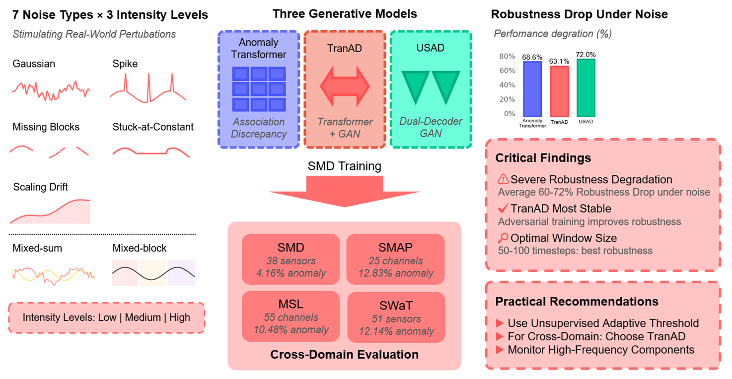
We systematically study robustness and detection performance of three representative generative models—AnomalyTransformer, TranAD, and USAD—against seven perturbation regimes: Gaussian, Spike, Missing blocks, Stuck-at-Constant, Scaling drift, and two composite settings Mixed-sum and Mixed-block. Each perturbation is evaluated at low, medium, and high intensities to emulate common degradation patterns such as stochastic noise, bursty outliers, partial outages, sensor freezes, slow drifts, and overlapping effects. This spectrum balances coverage (single vs. mixed) and controllability (intensity sweeps), enabling stress tests that are interpretable and reproducible.

To isolate robustness under domain shift, we train all models on SMD only (a widely used large-scale industrial benchmark [6]) and evaluate both in-domain and cross-domain on SMAP, MSL [7], and SWaT (industrial control testbed). This design reflects realistic deployment, where training data are often abundant for one plant or fleet but scarce elsewhere; robustness is then measured by performance retention under dataset shift rather than by re-training per domain. To contextualize generative models, we additionally include three baselines with distinct inductive biases—LSTM-AE (recurrent), TimesNet (period-aware convolution), and EWMA-Residual (statistical filtering)—so that sensitivity patterns can be compared across model families. For concise reporting, we identify top-2 baselines per dataset after benchmarking, while keeping all generative models throughout (details in Section 3).

Windowing, stride, and thresholding materially affect both latency and false alarms. Shorter windows reduce detection delay for transient anomalies but can miss long-horizon drifts; longer windows improve integration of slow trends at the cost of higher latency and memory/compute. We therefore adopt a baseline window of 50 (typical for short-latency monitoring) and vary to 100 and 200 to probe drift sensitivity. Stride 1 minimizes delay in baseline, while 5 offers a compute-efficient alternative for throughput-constrained deployments. Thresholds are compared across three regimes: Adaptive, which is re-estimated per test condition to reflect operational tuning; Clean-fixed, which is carried over from clean validation to quantify distribution-shift tolerance; and Unsupervised Adaptive, which is estimated from test data alone to emulate label-scarce settings [8]. This factorial variation aligns with how practitioners trade sensitivity vs. stability under resource and label constraints.

Beyond point-wise accuracy (F1, AUC), real operations care about when and how reliably alarms fire. We therefore report Core-5 metrics: F1, AUC, Range-F1 (segment-aware detection quality), mean DetectionDelay, and RobustnessDrop% (percentage performance loss from clean to noisy). To explain robustness patterns, we introduce architecture-level indicators: Residual High-Frequency Ratio (HFR), capturing the model’s tendency to amplify spurious high-frequency content under noise, and Representation Stability, quantifying the invariance of latent embeddings across clean vs. perturbed inputs [9,10]. These indicators connect outcome metrics to design choices such as attention concentration, adversarial training, and frequency selectivity, offering actionable insights rather than aggregate scores alone.

This work makes four contributions. First, we provide a comprehensive robustness evaluation of three generative and three baseline models under seven noise settings, including two mixed noise regimes with intensity sweeps. Second, we assess cross-domain generalization by training all models on SMD and then evaluating both in-domain (SMD) and cross-domain (SMAP, MSL, SWaT), thereby isolating robustness to dataset shift without re-training. Third, we analyze operational design trade-offs by varying window, stride, and thresholding in configurations that mirror latency and compute constraints in practice. Fourth, we augment standard accuracy metrics with robustness and architectural indicators (Core-5 plus HFR and Representation Stability), enabling diagnosis of model brittleness and architecture-specific failure modes. Together, these design choices aim to bridge the gap between clean-benchmark performance and deployable robustness in real-world time series environments.

2  Related Work

2.1 Generative AI-Based Time Series Anomaly Detection

Recent advances in deep learning have introduced generative AI models—primarily Transformer-based and Autoencoder-based approaches—that frequently surpass traditional statistical and classical machine learning methods in time series anomaly detection [11].

Among these, the AnomalyTransformer [3] extends the Transformer framework with an association discrepancy mechanism to better capture long-range temporal dependencies, thereby improving both detection and localization of anomalies. TranAD [4] combines Transformer layers with an adversarial Autoencoder framework, enhancing reconstruction fidelity and temporal feature learning in multivariate data. USAD [5] applies a GAN-inspired dual Autoencoder design that reinforces the modeling of normal patterns while suppressing anomalous signals.

Complementary to these architectures, Wang et al. introduce a cross-dimension attentive feature fusion network that integrates time- and frequency-domain representations for unsupervised time-series anomaly detection, improving multivariate representation quality [12].

These architectures demonstrate the strength of generative models in capturing complex temporal and inter-feature relationships. While large-scale evaluations confirm their effectiveness under clean conditions [1,2], their robustness against noisy or perturbed inputs has not been systematically examined.

2.2 Deep Learning and Statistical Benchmark Models

Beyond generative AI, a wide range of deep learning and statistical baselines have been proposed. LSTM-based Autoencoders and their variants remain widely used due to their ability to capture temporal dependencies through recurrent structures [7,13]. More recently, convolutional architectures such as TimesNet [14] and temporal decomposition models like Autoformer [15] extend the modeling capacity to capture both frequency-domain and long-horizon patterns. The Non-stationary Transformer further advances temporal modeling by explicitly addressing distribution shifts, providing additional robustness to evolving data distributions [16]. On the statistical side, residual-based detectors such as EWMA-Residual provide lightweight alternatives that remain competitive in scenarios with limited computational budgets [17]. These benchmark models serve as essential baselines for understanding the relative advantages of generative approaches and for identifying architecture-specific robustness trade-offs.

2.3 Robustness Evaluation under Noisy Conditions

Noise in time series data commonly arises from sensor malfunctions, communication disruptions, or environmental fluctuations. To reproduce such effects, synthetic noise models are widely adopted, including Gaussian noise (measurement variability), spike noise (abrupt sensor failures), missing blocks (communication losses), stuck-at-constant noise (frozen sensor readings), and scaling drift (gradual calibration errors) [8,18–20].

Beyond these individual noise types, real-world disturbances often occur in combination. To reflect this, composite perturbations such as Mixed-sum (additive overlap of Gaussian and spikes) and Mixed-block (simultaneous missing blocks with spikes or drifts) have been introduced in recent studies [20], providing more realistic stress tests. Noise intensity is typically parameterized into low, medium, and high levels, defined by statistical variance, spike ratio, or missing rate. This gradation enables reproducible sweeps of robustness sensitivity rather than binary “noisy vs. clean” comparisons.

Although several works propose robustness-oriented anomaly detection frameworks [21,22], most evaluations remain confined to individual models or restricted noise conditions. Large-scale benchmarks such as ADBench and TimeSeriesBench [23–25] emphasize algorithmic diversity and scalability, but they provide limited insight into robustness under structured noise. Furthermore, the interaction between model design factors—such as architectural inductive bias, window and stride settings, or thresholding strategies—and robustness remains underexplored [9,26]. Prior findings suggest that attention-based models may amplify high-frequency perturbations due to sensitivity to local misalignments, while Autoencoder-based models are often more vulnerable to block missingness or drift due to reliance on reconstruction continuity [8]. Yet, a systematic comparative analysis is lacking.

2.4 Adversarial and Attack-Oriented Perspectives

Complementary to random noise robustness, a growing body of research investigates adversarial attacks on time series anomaly detection models. Attack strategies such as gradient-based perturbations and adversarial patching have revealed vulnerabilities of anomaly detection models [27]. Generative attack networks (e.g., KAGAN) further expose weaknesses of both deep and generative architectures [28–30]. These works highlight that models trained under clean conditions may fail catastrophically under even small, targeted perturbations. While certified-robustness frameworks tailored to time-series models have begun to emerge [31], their integration into anomaly detection remains nascent and underexplored.

2.5 Summary of Research Gap

In summary, prior work establishes that generative AI models achieve state-of-the-art anomaly detection accuracy under clean conditions, while deep learning and statistical baselines continue to provide valuable points of comparison. However, comprehensive evaluations of robustness in noisy or adversarial environments are scarce. Specifically, there is limited evidence on how different generative architectures respond to varying noise types and intensities, how configuration choices such as window size, stride, and thresholding strategies affect robustness [32], and how robustness generalizes across domains such as SMD, SMAP, MSL, and SWaT [33]. Addressing this gap, the present study conducts a systematic robustness evaluation of three representative generative models—AnomalyTransformer, TranAD, and USAD—together with three baseline families, under seven noise types (including mixed perturbations), three intensity levels, and multiple experimental configurations.

3  Materials and Methods

3.1 Dataset Description

The datasets used in this study are summarized in Table 1. The baseline dataset is the Server Machine Dataset (SMD) [6], which contains multivariate server log time series collected from three server instances (machine-1-1, machine-1-2, machine-1-3). Each sequence comprises 38 sensor measurements, with anomalies introduced by diverse failure modes in real operations. Recent benchmarking studies report that SMD contains a total of 708,405 training and 708,420 testing sequences, with an anomaly rate of about 4.16% [34]. From a practical standpoint, server logs are representative of IT infrastructure monitoring, where anomaly detection is directly tied to service reliability and downtime prevention.

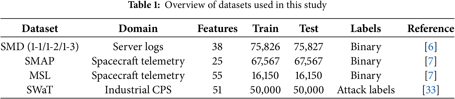
To broaden the evaluation scope and test cross-domain robustness, three additional benchmarks are included: SMAP and MSL from NASA spacecraft telemetry [7], and the Secure Water Treatment (SWaT) dataset from an industrial-scale cyber-physical system [33]. The SMAP dataset comprises 25 telemetry channels with 140,825 training and 444,035 testing sequences, while the MSL dataset includes 55 channels with 58,317 training and 73,729 testing sequences; their anomaly rates are approximately 12.83% and 10.48%, respectively [34]. Both represent safety-critical aerospace domains, where faults can cascade into mission failures. The SWaT dataset consists of 51 sensor and actuator variables collected from a real-world water treatment plant, with 495,000 training and 449,919 testing sequences, and an anomaly (attack) rate of 12.14% [35]. SWaT explicitly incorporates cyber-attacks, mirroring realistic industrial control system threats that anomaly detection must guard against. Together, these datasets span IT, aerospace, and industrial control scenarios, covering a spectrum of domains where robust anomaly detection is operationally critical.

For consistency across datasets, all time series are normalized and segmented into overlapping windows of length 50 time steps with stride 1. A window is labeled as anomalous if it contains at least one anomalous timestamp, a rule commonly used in prior studies to ensure early coverage of anomaly onset and to avoid discarding rare events. This baseline configuration reflects the need to balance timely detection (short windows for fast anomalies) and stable reconstruction (longer contexts for model training). A window length of 50 has become a common benchmark in prior studies [3,4]. To test robustness against long-term disturbances such as sensor drift, we extend the evaluation to windows of 100 and 200 steps. Stride 1 is adopted in the baseline to minimize Detection Delay, which is crucial in safety-critical applications, while stride 5 is additionally tested to simulate throughput-constrained scenarios common in industrial deployment.

To control experimental scale while retaining anomaly coverage, sub-sampling is applied to reduce redundancy. A proportional sampling rule is followed to preserve the original anomaly ratio, and a segment-based rule ensures that every anomaly event is retained at least once. This reflects real-world practices where rare faults must not be discarded but excessive normal sequences can be reduced without diagnostic loss. It is important to note that all datasets exhibit substantial class imbalance (e.g., anomaly rates typically 4%−13%). This imbalance affects metrics such as precision and recall, highlighting the necessity of evaluating multiple complementary measures.

Since datasets differ in feature dimensionality, a unified input space is required for cross-domain evaluation. We fix the input dimensionality to the 38-channel layout of the SMD dataset, since model architectures are trained under this configuration. Aligning other datasets to this target space avoids confounding effects of architectural re-design and ensures that robustness is evaluated under consistent model capacity. For datasets with fewer channels, we apply zero-padding (or repetition in the univariate case), which mirrors realistic missing-modality deployment scenarios [36,37]. For datasets with higher dimensionality, redundant sensors are truncated to enforce a fair comparison under the fixed model size, recognizing that more sophisticated alignment or feature-modelling methods exist [38,39]. This design reflects industrial practice: anomaly detection pipelines are often trained on one system and subsequently reused across heterogeneous environments with mismatched sensor layouts, where feature alignment is unavoidable [40]. Example segments from each dataset are illustrated in Fig. 1. For visualization, one representative univariate channel is selected per dataset, and anomalous intervals are highlighted in orange while normal regions are shown in blue. These plots are intended to illustrate dataset structure rather than replicate the exact experimental sampling protocol.

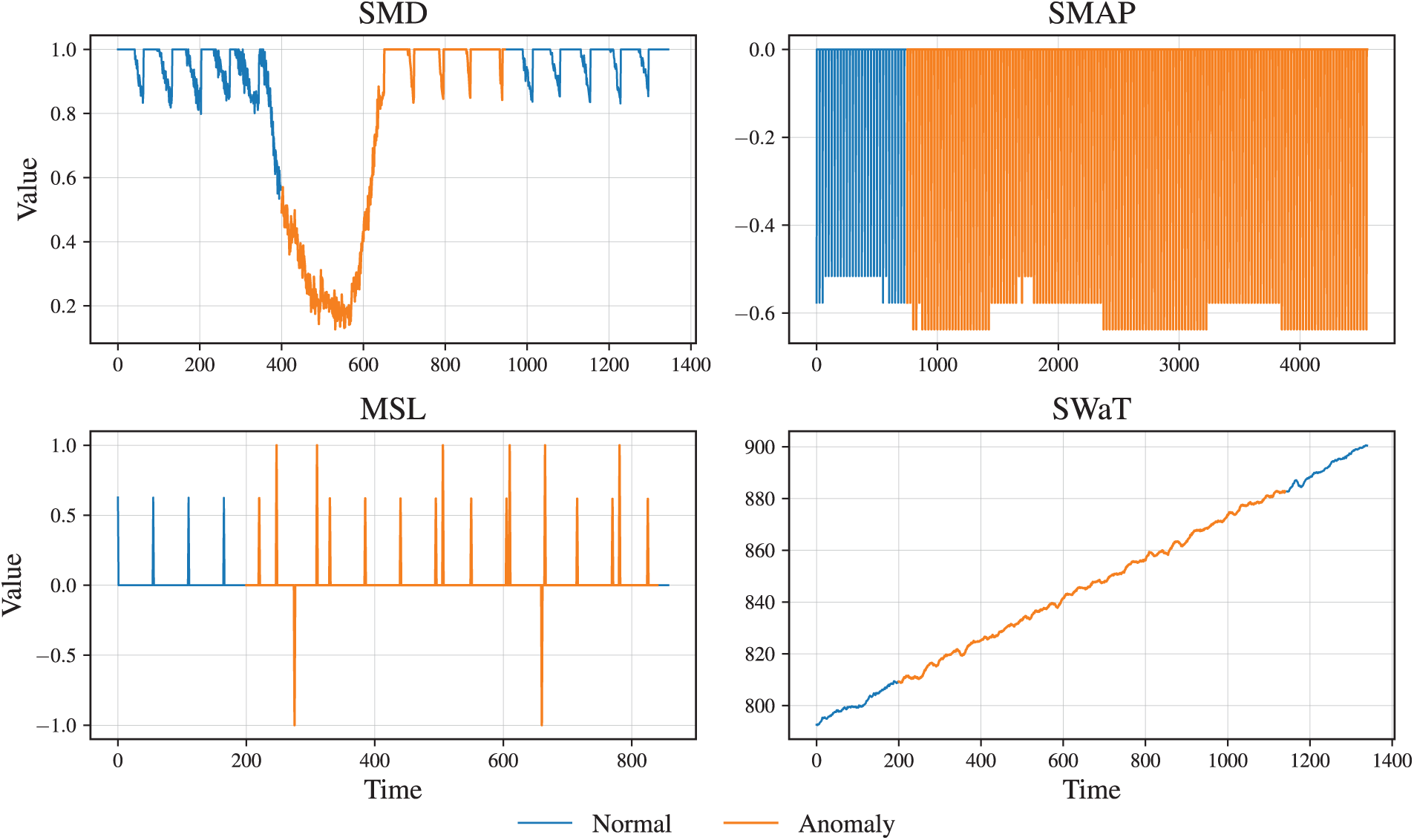
Figure 1: Example time series segments from four datasets

3.2 Experimental Settings

The baseline configuration trains all models on the SMD dataset using three server instances (machine-1-1, machine-1-2, machine-1-3). Time series are segmented into windows of length 50 with stride 1. A window length of 50 has been widely adopted in prior anomaly detection research [3,4], balancing the need to capture fast anomalies with the ability to learn stable temporal dependencies. Stride 1 is selected as the baseline to minimize Detection Delay, which is crucial in real-time IT monitoring and industrial process control, where missed detections of even a few seconds can lead to significant losses. Anomaly scores are binarized with an adaptive thresholding scheme [8], reflecting practical deployment where thresholds are adjusted dynamically to balance false alarms and missed detections.

For robustness evaluation, medium-intensity noise is injected, covering seven representative types: Gaussian, spike, missing blocks, stuck-at-constant, scaling drift, and two composite variants (Mixed-sum and Mixed-block). This design reflects realistic conditions in which measurement variability, sensor outages, calibration drifts, and overlapping disturbances may co-occur. All models are trained for 20 epochs under consistent settings for comparability. Transformer-based models use dmodel=32, nhead=2, and two encoder/decoder layers, while USAD employs a latent dimension of 32. Training is performed exclusively on SMD, while evaluation is extended to SMAP, MSL, and SWaT datasets, enabling cross-domain validation. This setting reflects real-world scenarios in which annotated training data are abundant in one environment but models must generalize to others with different feature layouts and anomaly dynamics. Evaluation metrics include the Core-5 set (F1, AUC, Range-F1, Detection Delay, Robustness Drop%) and two architecture-level indicators (Residual High-Frequency Ratio and Representation Stability).

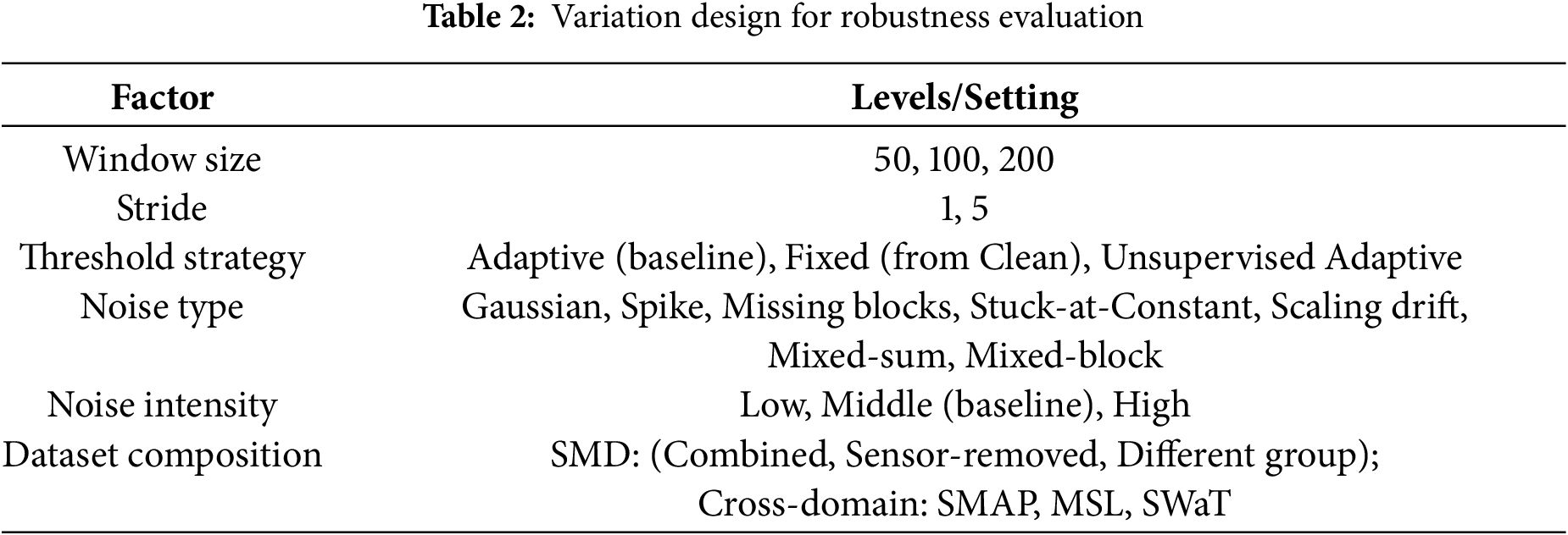
Variation experiments assess robustness under diverse conditions. Noise intensity is varied across low, medium, and high levels, corresponding to realistic environments ranging from minor calibration errors to severe sensor malfunctions, consistent with prior robustness evaluation practices in noise-contaminated time series anomaly detection [10,19]. Window sizes of 50, 100, and 200 are examined: shorter windows enable rapid detection in IT log monitoring, whereas longer windows capture gradual anomalies such as drift in industrial sensors. Stride values of 1 and 5 are tested: stride 1 ensures immediate responsiveness, while stride 5 simulates deployment in bandwidth- or compute-constrained systems, where subsampling is necessary for throughput [2]. Threshold strategies are compared across three regimes: adaptive thresholds re-estimated per test condition to reflect operational tuning, fixed thresholds derived from clean validation data to quantify distribution-shift tolerance, and unsupervised adaptive thresholding estimated from test data alone to emulate label-scarce environments [9]. Dataset composition is also varied. Within SMD, three settings are tested: combined use of the three baseline servers, sensor-removed subsets (for example, machine-1-1 and machine-1-3) to simulate partial observability due to sensor failures, and a different server group (machine-2-1, machine-2-2, machine-2-3) to test generalization to related but distinct machines. Cross-domain evaluation further includes SMAP, MSL, and SWaT, ensuring robustness is tested across aerospace telemetry and industrial CPS data. This comprehensive variation design mirrors deployment conditions in which models must remain reliable across heterogeneous domains, incomplete sensor coverage, and a range of noise severities, as summarized in Table 2.

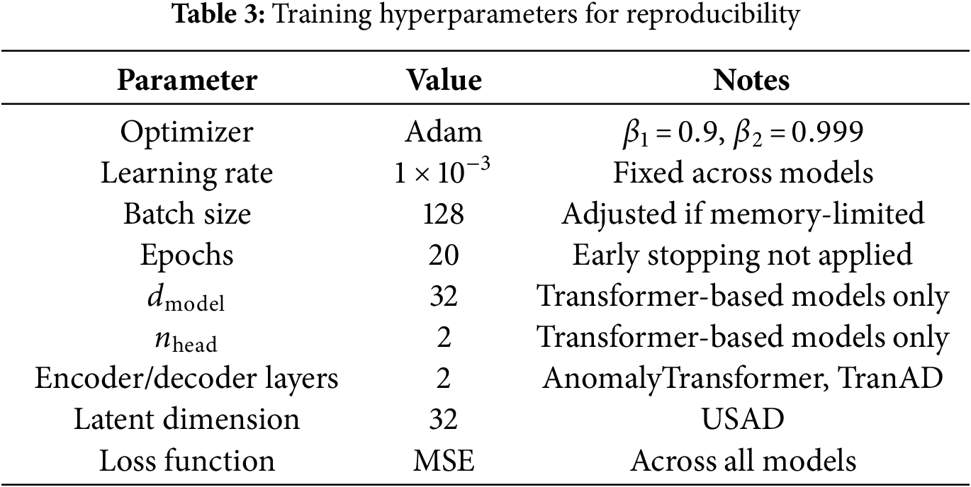
The training and evaluation regime follows the principle of training once on clean SMD data and then directly evaluating under all variation conditions without retraining. This design isolates the effect of perturbations and temporal granularity from the confounding influence of model re-optimization. When the evaluation window size differs from the training configuration, input sequences are adjusted by simple truncation (if longer) or zero-padding (if shorter), mirroring practical deployment where window mismatch is handled with minimal preprocessing. Feature dimensionality is aligned by repetition, truncation, or padding as described in Section 3.1. The hyperparameter settings are kept consistent across models unless otherwise noted, as listed in Table 3.

3.3 Noise Injection Methodology

To emulate disturbances commonly observed in cyber-physical and industrial monitoring environments, seven representative noise types are injected into the test data. These include five single-source perturbations (Gaussian, spike, missing blocks, stuck-at-constant, scaling drift) and two mixed variants (Mixed-sum and Mixed-block). The parameterization follows prior robustness-oriented studies in anomaly detection [18–20], and additional justification is provided in line with realistic sensor failure modes [8,41]. For example, Gaussian noise is zero-mean with variance scaled to signal magnitude, ranging from σ=0.01 (minor calibration offsets) to σ=0.10 (severe instability). Spike noise is injected as short-duration, high-amplitude transients, with both number and amplitude increasing by intensity level. Missing blocks emulate communication dropouts with block lengths of 5, 15, and 30 steps. Stuck-at-Constant noise simulates frozen sensors where values remain clamped for 10, 30, or 60 steps. Scaling drift gradually applies a multiplicative factor step by step, from 0.001 per step (slow drift) to 0.01 per step (rapid compounding bias). Mixed-sum combines two or three of these perturbations simultaneously, while Mixed-block partitions a sequence so that different segments are distorted by different noise types.

Each noise type is evaluated under three intensity levels (low, middle, high), as summarized in Table 4. Parameter values are selected to reflect practical ranges documented in sensor reliability studies [1,11,41]. Low intensity corresponds to minor distortions that preserve temporal structure, middle intensity introduces partial ambiguity, and high intensity produces severe disruptions that challenge model stability. All intensity levels are consistently applied across window sizes (50, 100, 200) and stride settings (1, 5), ensuring reproducibility and comparability of results. For stochastic processes such as spike locations or missing blocks positions, a fixed random seed is used to guarantee experiment reproducibility. Fig. 2 provides illustrative examples, showing clean signals in blue and perturbed signals in orange.

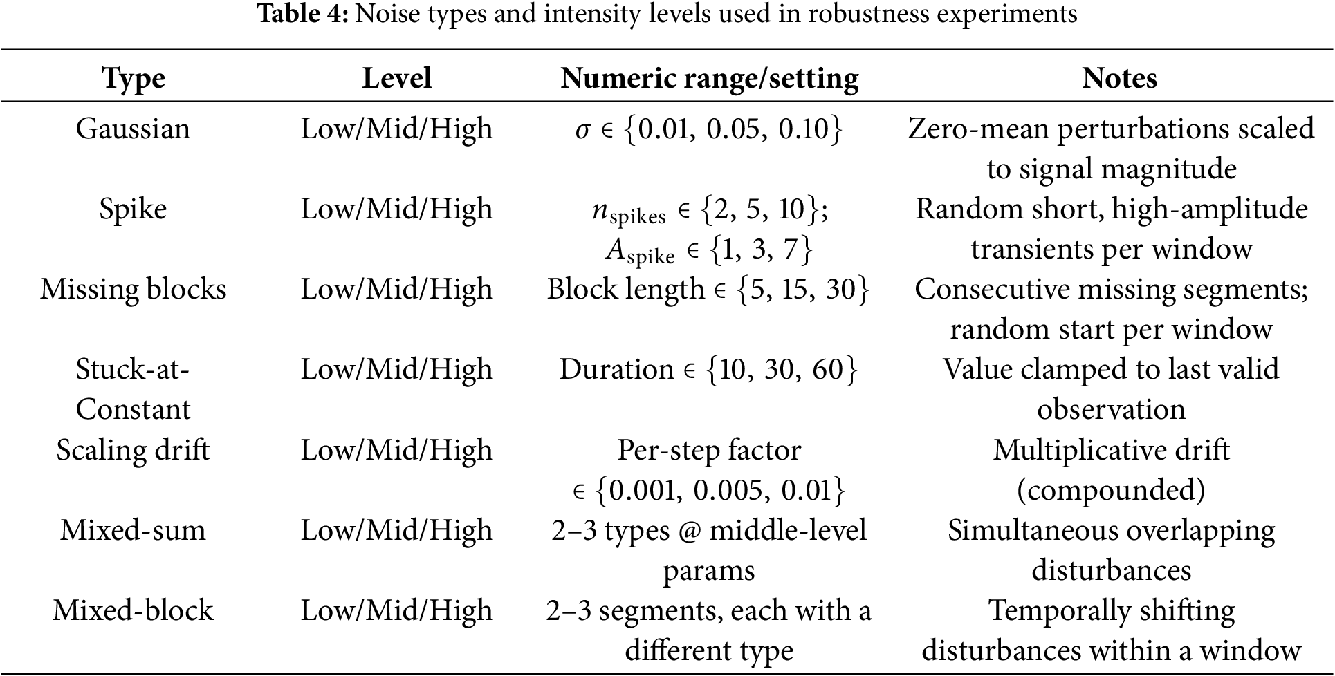
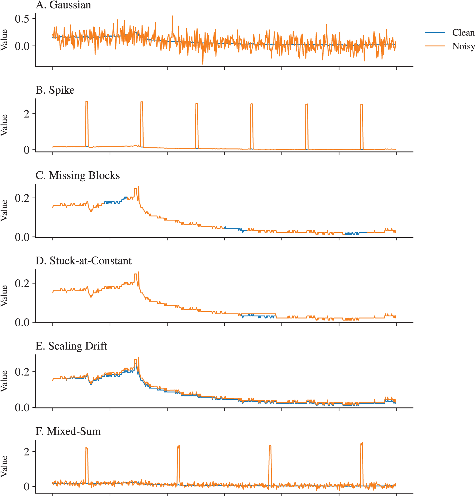
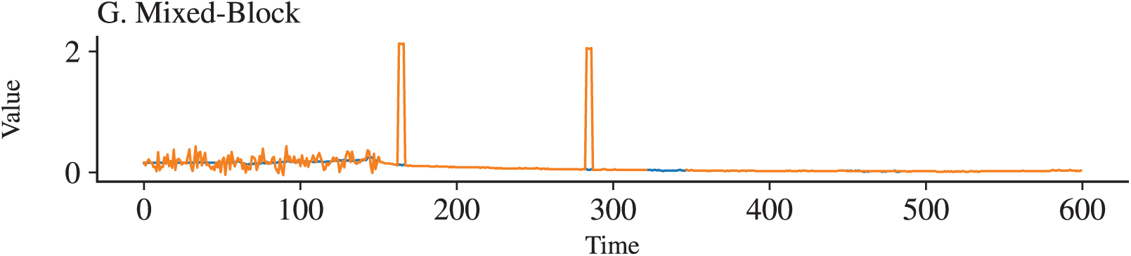
Figure 2: Illustration of seven representative noise types

3.4 Window and Stride Variation

To systematically assess how temporal granularity affects robustness, we vary the sliding window size and stride beyond the baseline configuration of 50 time steps with stride 1. This choice follows prior anomaly detection benchmarks such as AnomalyTransformer [3] and TranAD [4], where a window of 50 has become a standard reference for evaluating both point-level and contextual anomalies. In our experiments, larger windows of 100 and 200 steps are additionally examined to capture long-term dependencies and gradual distortions.

The variation in window size highlights an important trade-off. Short windows, such as 50 steps, provide rapid responsiveness and are well suited to domains such as server monitoring (SMD) and critical infrastructure (SWaT), where anomalies may manifest as transient spikes, short-lived failures, or abrupt attacks. Larger windows of 100 to 200 steps extend the receptive field, enabling models to capture seasonal effects and drift patterns that characterize telemetry from aerospace domains (SMAP, MSL) and industrial processes. While short windows minimize Detection Delay, longer windows improve stability under slowly evolving disturbances such as sensor calibration drift [14,42]. From an industrial perspective, selecting an appropriate window size mirrors operational choices: real-time intrusion detection favors shorter contexts, whereas predictive maintenance and trend analysis benefit from longer horizons.

The variation in stride is examined through two settings, 1 and 5, to reflect the balance between detection timeliness and computational efficiency. A stride of 1 minimizes Detection Delay, which is essential in safety-critical environments such as water treatment control loops in SWaT or server downtime prevention in SMD. In contrast, a stride of 5 reduces redundant computations by sampling fewer overlapping windows, which is acceptable in slower-evolving domains such as SMAP and MSL where anomalies unfold gradually [24]. Very large strides, such as 10 or more, are excluded, as they risk overlooking short-lived but operationally significant events, consistent with prior evaluations [8,26].

The labeling rule ensures that any window containing at least one anomalous timestamp is labeled as anomalous. This approach preserves even rare but critical deviations in evaluation, mirroring real-world monitoring practices where a single fault within a short interval may trigger an alarm.

Experimental consistency is maintained by applying all noise types and intensity levels uniformly across window sizes (50, 100, 200) and stride settings (1, 5). This guarantees fair comparison and isolates the effect of temporal granularity from other confounding factors. The design thus provides a balanced view of how anomaly detectors trade off sensitivity, robustness, and efficiency across different application scenarios.

3.5 Model Architectures

This study focuses on three representative generative AI-based anomaly detection models—AnomalyTransformer, TranAD, and USAD—that capture different inductive biases and architectural designs. To contextualize their performance, three benchmark baselines (LSTM-AE, TimesNet, and EWMA-Residual) are included, covering recurrent, convolutional, and statistical paradigms. These baselines are not the primary research targets but serve as essential comparison points, with the stronger ones highlighted in cross-domain analysis. The selection of models balances depth, by comparing generative AI designs, with breadth, by contrasting against established baselines. An overview of these architectures is illustrated in Fig. 3.

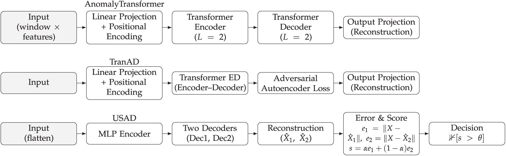
Figure 3: Overview of model architectures

•   AnomalyTransformer [3]: A Transformer encoder—decoder with an association discrepancy mechanism, designed to capture both long-range temporal dependencies and local–global correlations. This architecture is suited to domains such as data center monitoring or industrial IoT, where anomalies may arise from gradual drifts or distributed failures that require context-aware modeling.

•   TranAD [4]: An adversarial Autoencoder framework enhanced with Transformer layers. By integrating adversarial reconstruction loss, TranAD improves robustness against distributional shifts in multivariate signals, making it particularly relevant for manufacturing and IoT scenarios with complex correlations across sensors.

•   USAD [5]: A dual-decoder GAN-inspired Autoencoder that reconstructs normal sequences while penalizing deviations. This design directly targets the modeling of normality, making it effective for detecting distorted or frozen sensor signals often observed in industrial equipment.

For benchmarking, we additionally include the following baselines:

•   LSTM-AE [7,13]: A recurrent encoder—decoder baseline that captures sequential dependencies. It remains widely used in practice due to its simplicity and interpretability, making it useful for industrial fault detection where legacy RNN models are often deployed.

•   TimesNet [14]: A convolutional architecture that models temporal 2D variations through multi-period filters. It provides strong general-purpose performance and is particularly relevant for telemetry or financial series where periodic patterns dominate.

•   EWMA-Residual [17]: A statistical moving-average method applied to residual signals. While lightweight, it offers practical utility in real-time monitoring with limited compute budgets, such as network traffic or embedded industrial systems.

The training configuration is standardized to ensure fair comparison. All models are implemented in PyTorch and trained under comparable settings using the Adam optimizer with a learning rate of 1×10−3, batch size 128, and mean squared error loss. Training is conducted for 20 epochs on GPUs with early stopping disabled to preserve consistency across models. For Transformer-based models, the hidden dimension is set to dmodel=32, with nhead=2, feedforward dimension 128, and two encoder/decoder layers. USAD employs a latent dimension of 32 with two parallel decoders. These configurations follow prior anomaly detection benchmarks and strike a balance between stability and computational feasibility in industrial deployment [8,23].

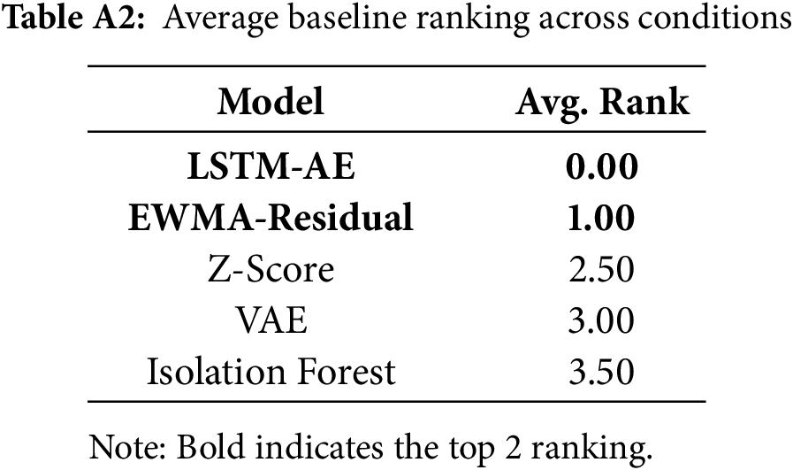
The baseline selection process screened multiple candidates, including LSTM-AE, TimesNet, EWMA-Residual, Z-Score, VAE, and Isolation Forest. Among these, only LSTM-AE and EWMA-Residual were consistently ranked as the top-2 performers across both clean and noisy conditions (Appendix A). These two are therefore retained for cross-domain comparisons, ensuring both methodological diversity and empirical strength.

3.6 Evaluation Protocol

All models are trained once on clean data from the baseline SMD composition and then evaluated across all variation conditions, including noise type and intensity, window and stride settings, and cross-domain datasets. This design reflects realistic industrial constraints: anomaly detectors are typically trained on historical clean logs, while deployment environments often involve unforeseen noise or domain shifts. By fixing the training condition, robustness degradation can be explicitly quantified without conflating it with retraining or domain adaptation effects.

A crucial consideration lies in how robustness is quantified. Recent benchmarking initiatives in time series anomaly detection, such as RobustAD, TSB-UAD, and more recent efforts like TimeSeriesBench and TAB, have shifted away from reliance on a single detection score toward multi-metric evaluation protocols [8,24,26,43]. This transition reflects a growing consensus that no single metric can adequately capture the multi-faceted requirements of anomaly detection systems [9,44]. In this context, the Core-5 suite has emerged as a representative and increasingly adopted basis for robustness studies. It consolidates complementary perspectives into a cohesive evaluation framework: detection accuracy (F1, AUC), segment-level coverage (Range-F1), temporal responsiveness (Detection Delay), and robustness under perturbations (Robustness Drop%, defined as the relative change in F1 between clean and noisy conditions). Together, these metrics span the three dimensions most critical to deployment—performance, latency, and robustness—offering a principled alternative to narrow, single-metric reporting.

From a practical standpoint, Core-5 also aligns with operational priorities in industrial monitoring: knowing not only how many anomalies are detected, but also when alarms are raised and how sensitive performance is under noise. These aspects are often more consequential than marginal improvements in aggregate accuracy [45]. To further contextualize robustness at the architectural level, we additionally introduce two architecture metrics: Residual High-Frequency Ratio (HFR) and Representation Stability (RS). While Core-5 evaluates external performance outcomes, these metrics diagnose internal model behavior under perturbations, shedding light on how inductive biases influence robustness. This combined protocol ensures both comprehensive benchmarking and interpretability of robustness differences across models. The end-to-end evaluation workflow is summarized in Fig. 4.

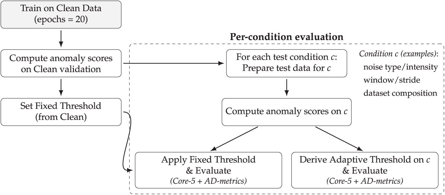
Figure 4: Evaluation protocol

•   Thresholding strategies. Three strategies are compared, each corresponding to a distinct deployment scenario:

1.    Clean-Fixed Threshold: Determined once from clean validation data and applied unchanged across all conditions. This reflects environments where threshold re-tuning is infeasible due to limited domain expertise or strict operational constraints.

2.    Adaptive Threshold: Re-estimated independently for each test condition. This represents an upper bound on achievable performance when recalibration is feasible, such as laboratory settings or expert-assisted monitoring.

3.    Unsupervised Adaptive Threshold: Estimated directly from the test distribution without reference to clean validation, using heuristics such as statistical percentiles or POT methods. This enables fully unsupervised deployment in settings where labeled data are unavailable.

•   Evaluation metrics. Two complementary groups of metrics are employed:

1.   Core-5: (F1,AUC,Range-F1,Detection Delay,Robustness Drop%). This suite jointly captures detection accuracy, temporal responsiveness, and robustness under distributional shifts. Prior studies have emphasized that relying only on F1 or AUC is insufficient for robustness evaluation [8,9], motivating the adoption of this multi-faceted set as a more principled basis for comparison.

–   F1: Harmonic mean of Precision and Recall at the chosen threshold.

–   AUC: Area under the ROC curve, threshold-independent measure of separability.

–   Range-F1: Segment-level F1, counting each contiguous anomaly interval as one unit to avoid over-penalizing Detection Delay values.

–   Detection Delay: Average number of time steps between the start of an anomaly and the first correct detection within that interval.

–   Robustness Drop%: Relative performance degradation between clean and noisy test conditions, ΔF1/F1clean×100%.

2.   Architecture metrics: Residual High-Frequency Ratio (HFR) and Representation Stability (RS). These provide structural insights into how models behave under noise or domain shifts, revealing brittleness in latent representations that may not be visible from detection metrics alone.

–   HFR: Ratio of high-frequency energy in residual (error) signals, quantifying sensitivity to spurious fluctuations.

–   RS: Cosine similarity of latent representations across clean vs. perturbed inputs, measuring invariance of embeddings under noise.

4  Results

4.1 Overall Performance in Clean and Noisy Conditions

Table 5 summarizes the baseline Core-5 results for six representative models across the four datasets. Clean values (F1, AUC, Range-F1, mean Detection Delay) are reported alongside the mean Robustness Drop% across all single-noise perturbations. For readability in Table 5, we abbreviate Detection Delay as Delay and Robustness Drop% as Drop%. While these averages provide a compact view of robustness, it should be noted that mixed noise settings (Mixed-sum, Mixed-block) cause even larger degradations, as further discussed in Section 4.3. Within each dataset block of Table 5, we bold the best value per column (F1/AUC/Range-F1: higher is better; Delay: lower is better; Drop%: the smallest non-negative value is considered best; negative values are reported but not treated as improvements).

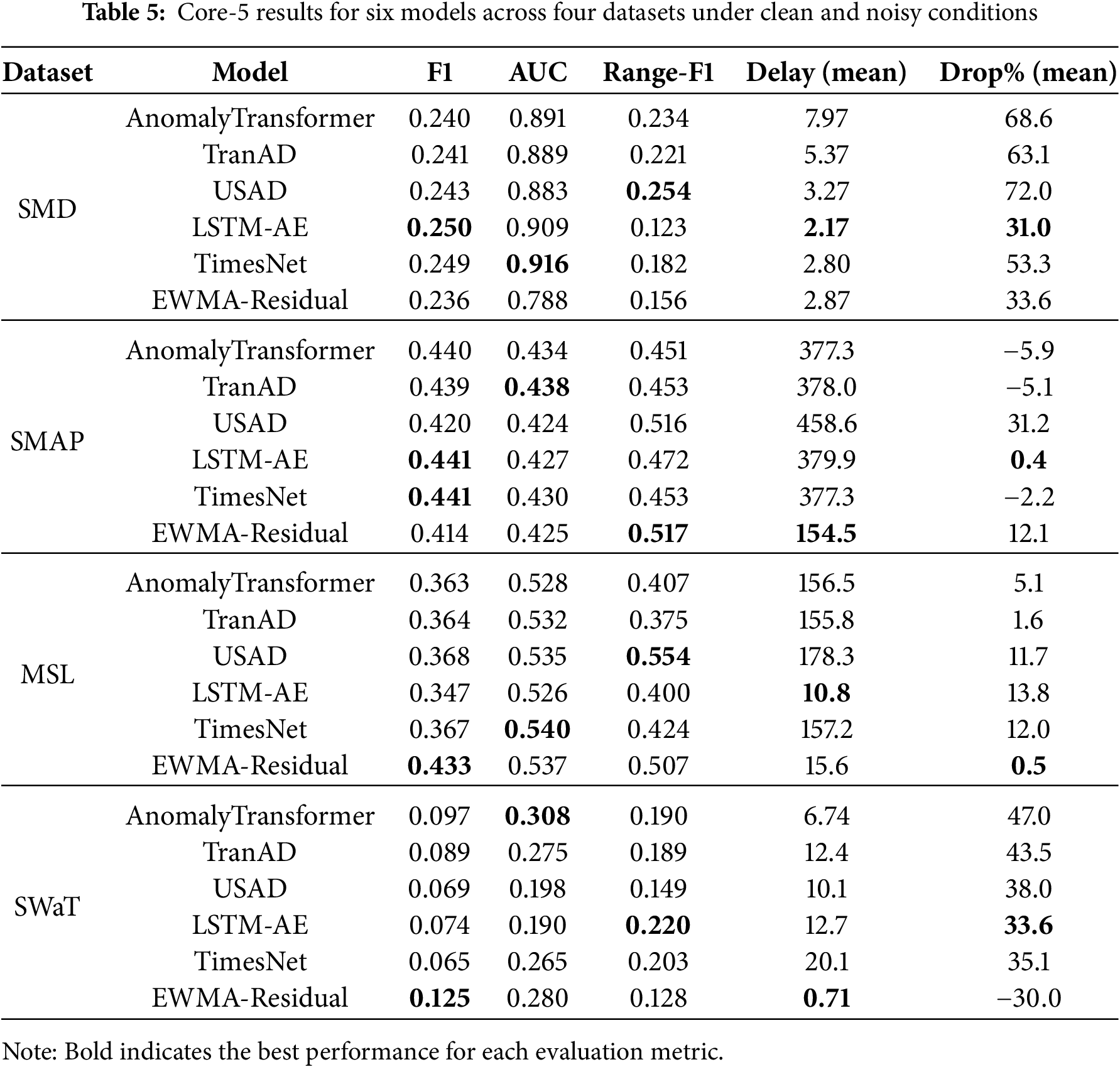
Clean performance shows that the three generative models exhibit comparable F1 scores on SMD (0.23–0.25) and moderate performance on MSL and SMAP (0.36–0.44), but all struggle on SWaT (F1<0.12). AnomalyTransformer and TranAD achieve strong AUC values on SMD (0.85–0.92), while USAD reaches its best F1 on MSL (0.368). Range-F1, however, diverges across models: USAD attains the highest Range-F1 on MSL (0.554), indicating superior segment-level detection coverage, whereas AnomalyTransformer remains relatively low (0.234 on SMD). Baselines show heterogeneous patterns: TimesNet offers slightly higher clean AUC (for example, 0.916 on SMD), while LSTM-AE and EWMA-Residual provide shorter delays (under 3 timesteps), which is industrially relevant since faster anomaly signaling directly reduces downtime costs.

Robustness under noise reveals substantial differences among generative models. AnomalyTransformer suffers steep degradation on SMD (Robustness Drop% =68.6), reflecting high sensitivity to block and drift perturbations. TranAD demonstrates resilience, particularly on MSL (Robustness Drop% =1.6), where its adversarial regularization stabilizes decision boundaries. USAD, despite competitive clean accuracy, shows the largest average Robustness Drop% (72.0 on SMD), and is especially vulnerable to structured and mixed noise. These Robustness Drop% values highlight real-world consequences: higher degradation implies more frequent retraining and higher operational maintenance costs. Baselines occasionally surpass generative models: LSTM-AE maintains moderate stability on SMD (Robustness Drop% =31.0), while EWMA-Residual improves under SWaT (Robustness Drop% =−30.0), suggesting that lightweight residual filtering can adapt more effectively to unstable telemetry domains. Negative values of Robustness Drop% indicate rare cases where noisy conditions yield slightly higher scores than clean, often due to thresholding effects or the smoothing of unstable signals (as observed on SMAP and SWaT). Such effects should be interpreted as dataset—model interactions rather than genuine robustness improvements [9].

Cross-domain generalization highlights further challenges. When trained on SMD and tested on other domains, generative models generalize poorly to SWaT (all F1<0.10), underscoring sensitivity to domain shift. EWMA-Residual and LSTM-AE, although weaker in clean accuracy, maintain relatively lower Robustness Drop% values, offering stability advantages. On SMAP, performance fluctuations are amplified due to lower representation stability, yet TranAD sustains competitive results (AUC 0.438, Robustness Drop% =−5.1), reflecting its stronger transferability.

Connection to architecture metrics shows that patterns in Core-5 align with structural indicators. For example, AnomalyTransformer’s high Robustness Drop% on SMD corresponds to elevated residual high-frequency ratios (HFR), while USAD’s instability on SMAP coincides with low representation stability (RS below 0.4). These observations suggest that robustness degradation often originates from unstable latent features, reinforcing the importance of combining Core-5 with architecture-level diagnostics. Detailed interpretations are provided in Section 5.3.

In summary:

•   AnomalyTransformer: strong clean accuracy but sharp robustness degradation (Robustness Drop% up to 68), highlighting its sensitivity to structured noise.

•   TranAD: most robust overall, especially on MSL (Robustness Drop% ≈1.6), with adversarial training reducing degradation.

•   USAD: competitive clean accuracy but the most vulnerable to structured and mixed perturbations, showing the largest Robustness Drop%.

•   Baselines: TimesNet balances high clean AUC with moderate robustness, LSTM-AE demonstrates partial stability, and EWMA-Residual adapts unexpectedly well in SWaT, offering lightweight robustness in volatile domains.

4.2 Impact of Dataset Composition

Dataset composition substantially shapes both clean performance and noise robustness. Under a unified baseline configuration, we compare SMD in-domain cases (baseline, SMD with sensor removal, and SMD with server group variation) against cross-domain shifts to SMAP, MSL, and SWaT. A consolidated comparison is presented in Fig. 5.

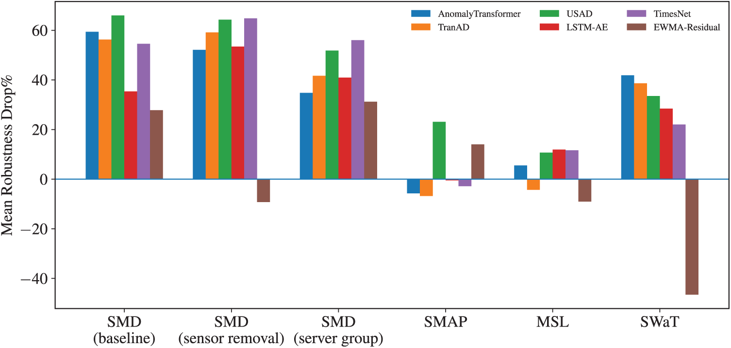
Figure 5: Robustness across dataset compositions

In the SMD in-domain setting, generative and deep models exhibit large robustness degradation on average: AnomalyTransformer and TranAD show mean Robustness Drop% values of around 59 and 56, USAD around 66, and TimesNet around 55, while LSTM-AE is lower but still sizable at about 35. EWMA-Residual is relatively more stable at about 28. Sensor removal generally worsens performance for representation-heavy models, with AnomalyTransformer, TranAD, USAD, and TimesNet all above 52, whereas EWMA-Residual remains stable. By contrast, server group variation mitigates degradation somewhat for AnomalyTransformer and TranAD, with mean Robustness Drop% values of about 35 and 42, though TimesNet remains highly sensitive at about 56. These results show that even within the same dataset family, changes in feature composition substantially affect model stability. Detection Delay values also diverge: residual baselines sustain short delays under three timesteps, while Transformer-based models incur longer latencies, highlighting a potential trade-off between representation power and operational responsiveness.

On SMAP, several models show small or even negative mean Robustness Drop% values, with AnomalyTransformer at about −5.7, TranAD at −6.8, TimesNet at −2.8, and LSTM-AE at −0.5, while USAD and EWMA-Residual deteriorate with means of +23.1 and +14.0. On MSL, EWMA-Residual again remains strong with about −9.0, TranAD is mildly robust with −4.3, and the others degrade moderately, with AnomalyTransformer, USAD, TimesNet, and LSTM-AE all around 5 to 12. These negative values do not imply true robustness improvements; rather, they reflect thresholding effects or the smoothing of unstable telemetry signals under noise. Range-F1 trends further confirm that segment-level detection coverage is inconsistent across architectures, with USAD showing higher coverage but at the cost of larger Robustness Drop% values, while simpler baselines provide narrower but more stable coverage. This suggests that in smaller-variable, higher-anomaly-rate telemetry, lighter models or residual baselines can match or surpass complex architectures in robustness.

On SWaT, the ranking shifts. Transformer or reconstruction models incur large Robustness Drop% values, with AnomalyTransformer at about 41.9, TranAD at 38.6, USAD at 33.5, LSTM-AE at 28.4, and TimesNet at 22.0, while EWMA-Residual is exceptionally stable with a strongly negative mean Robustness Drop% of about −46.5. Attack-driven anomalies coupled with control dynamics appear to favor residual-style detectors under noise, while complex models remain sensitive to thresholding around perturbed residuals. From an industrial perspective, this highlights that models tuned for IT infrastructure monitoring (SMD) or space telemetry (SMAP and MSL) do not directly transfer to cyber-physical control systems like SWaT, where fast detection and stable filtering are more valuable than high clean accuracy.

In summary:

•   In-domain feature composition (sensor removal, server group) penalizes representation-heavy models but leaves residual baselines stable, while also increasing Detection Delay for Transformer-based methods.

•   Cross-domain shifts interact with dataset scale and anomaly density: telemetry datasets (SMAP/MSL) favor lighter models, while attack-driven SWaT favors residual detectors.

•   Negative values of Robustness Drop%, observed mainly in SMAP and MSL, arise from threshold adaptation or noise smoothing effects and should not be interpreted as genuine robustness gains.

4.3 Impact of Noise Type and Intensity

Figs. 6 and 7 compare the three main models under representative noise settings with varying intensity levels. Spike noise is chosen as the most disruptive case, while Mixed-sum represents composite perturbations. Additional figures for the remaining noise types are reported in Appendix B.

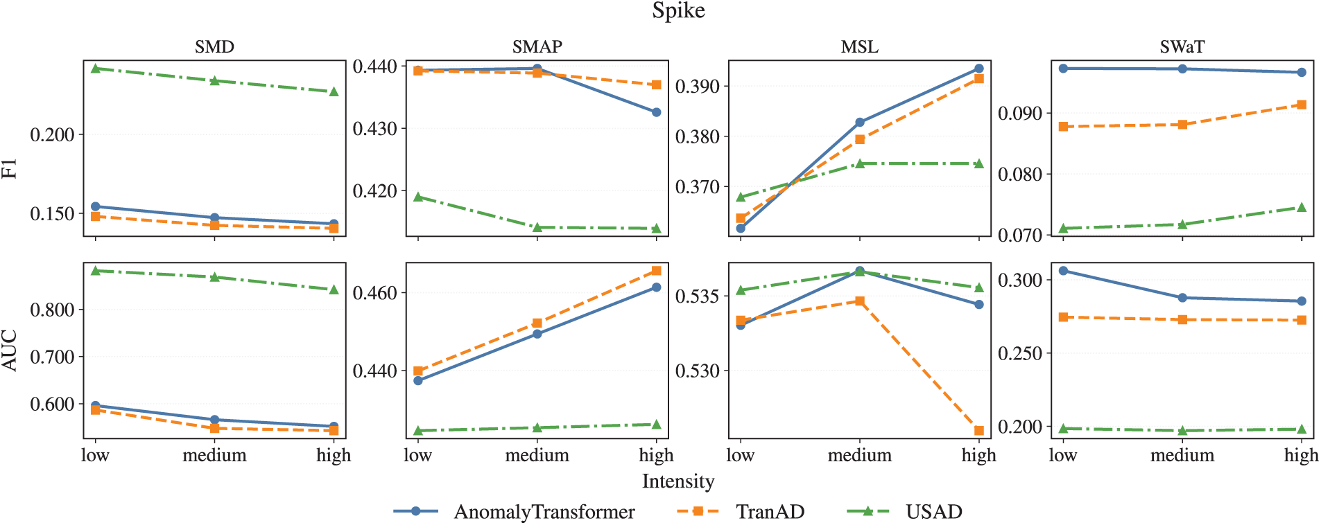
Figure 6: Model performance under Spike noise across intensity levels

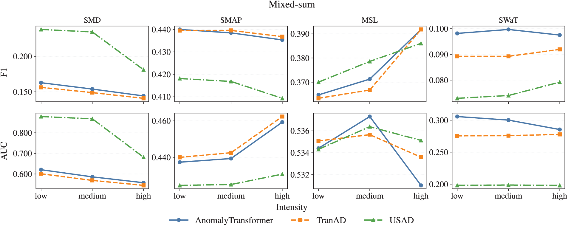
Figure 7: Model performance under Mixed-sum noise across intensity levels

Under Gaussian and Scaling drift perturbations, all models exhibit relatively mild sensitivity to intensity. Even at high levels, F1 remains around 0.21–0.25 and AUC above 0.85, suggesting that smooth or gradual distortions exert limited disruption. Missing blocks cause stronger degradation at higher intensity, mainly by reducing precision (down to 0.219–0.228 for AnomalyTransformer and TranAD), whereas stuck-at-constant perturbations show minimal dependence on intensity.

Spike noise, in contrast, produces the steepest intensity-driven collapse. Fig. 6 shows that as intensity increases, AnomalyTransformer and TranAD both deteriorate sharply, with F1 falling below 0.10 and AUC approaching 0.55 at high intensity. USAD also declines, but maintains comparatively higher robustness (F1≈0.210, AUC ≈0.801), underscoring its relative resilience. Mixed-sum perturbations (Fig. 7) show similar patterns: both Transformer-based models suffer strong declines, while USAD degrades more gradually, retaining a relative advantage.

In summary:

•   Gaussian and Scaling drift are relatively benign even at high intensity.

•   Missing blocks primarily harm precision at higher levels.

•   Spike and Mixed perturbations are most detrimental, producing steep intensity-driven deterioration.

•   USAD demonstrates the strongest robustness across intensities, particularly under challenging Spike and Mixed conditions.

4.4 Impact of Window Size and Stride Variation

Figs. 8 and 9 summarize the influence of window size and stride on robustness across all datasets, evaluated with noise-averaged Core-5 metrics.

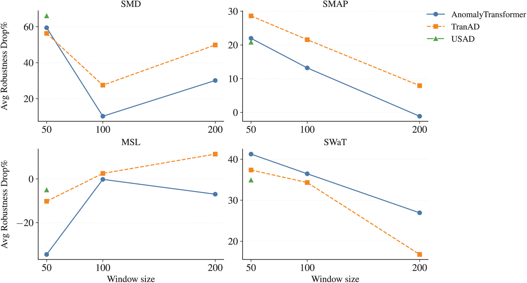
Figure 8: Effect of window size on robustness (mean Robustness Drop%)

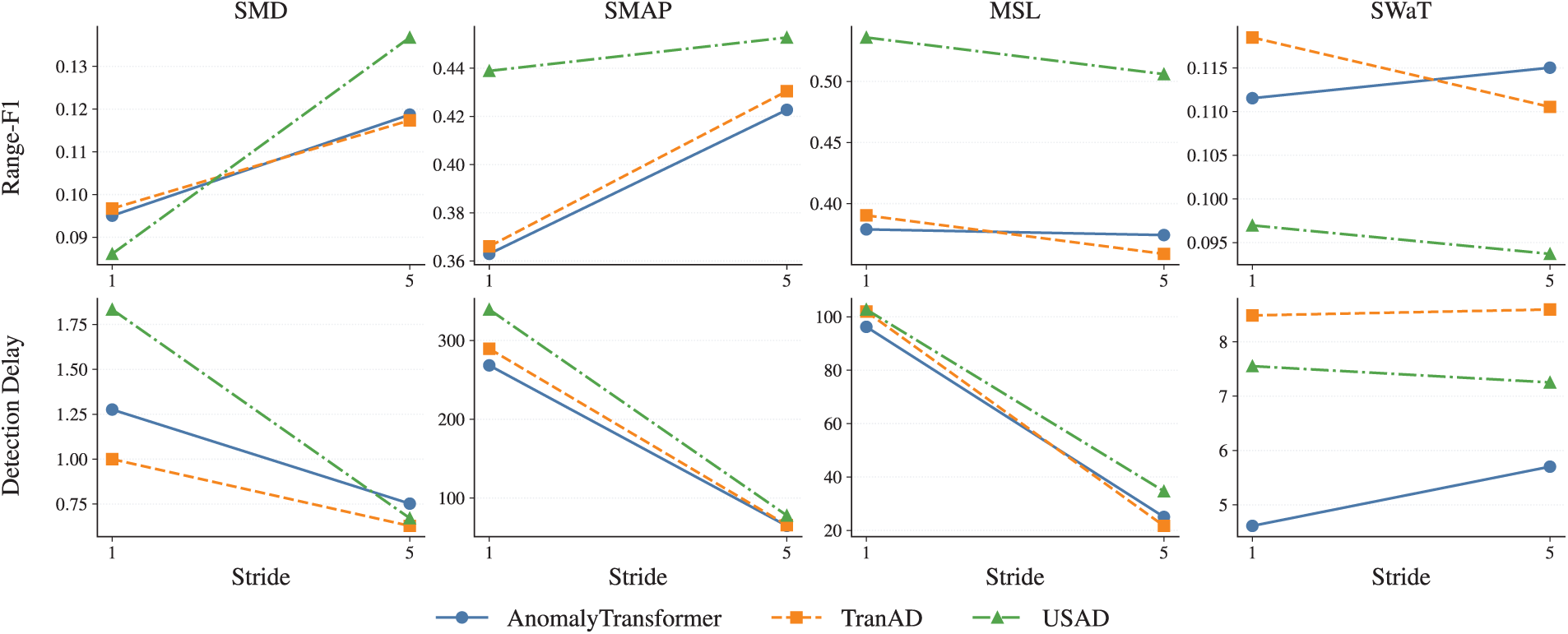
Figure 9: Impact of stride on Range-F1 and detection delay

For window size, Fig. 8 reports the mean Robustness Drop% for AnomalyTransformer, TranAD, and USAD under stride =1. The effect of window length is clearly non-linear. Moderate windows (50–100) generally achieve the lowest degradation, while very large windows (200) tend to increase drop rates, especially for AnomalyTransformer. For example, on SMD the drop for AnomalyTransformer rises from ∼69% at w=50 to over 75% at w=200, indicating that excessive context dilutes anomaly sensitivity. TranAD follows a similar trend with smaller magnitude, whereas USAD remains relatively flat but never reaches the best robustness levels. These results highlight that enlarging temporal context beyond a certain point does not guarantee improved robustness and may instead amplify noise sensitivity.

For stride, Fig. 9 compares stride =1 and =5 at fixed w=50, using paired slope plots of Range-F1 and Detection Delay. The impact is modest overall: Range-F1 decreases only slightly when moving to stride =5, while delay tends to increase marginally (e.g., ∼+0.3 steps on average for SMD). This indicates that temporal down-sampling does not dramatically alter robustness but can trade a small loss in detection accuracy for computational savings. Model-wise, AnomalyTransformer is more sensitive to stride increases in Range-F1, while TranAD maintains stable values and USAD shows consistently longer delays.

In summary:

•   Window size is the dominant factor: mid-range (50–100) yields the best robustness, while very large windows (200) amplify noise sensitivity.

•   Stride has minor influence: increasing stride modestly reduces Range-F1 and slightly increases delay, but overall robustness remains stable.

4.5 Impact of Thresholding Strategies

Table 6 summarizes the performance of three thresholding strategies—Clean-fixed, simple Adaptive, and Unsupervised Adaptive—across models and datasets. Reported are F1-score, AUC, and Range-F1 under both clean and noise-averaged conditions. Boldface highlights the best-performing threshold within each model—dataset–condition block.

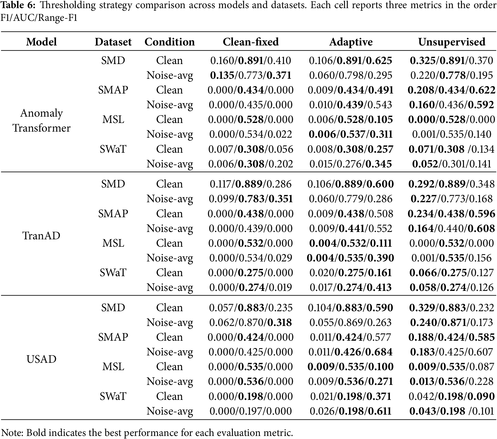
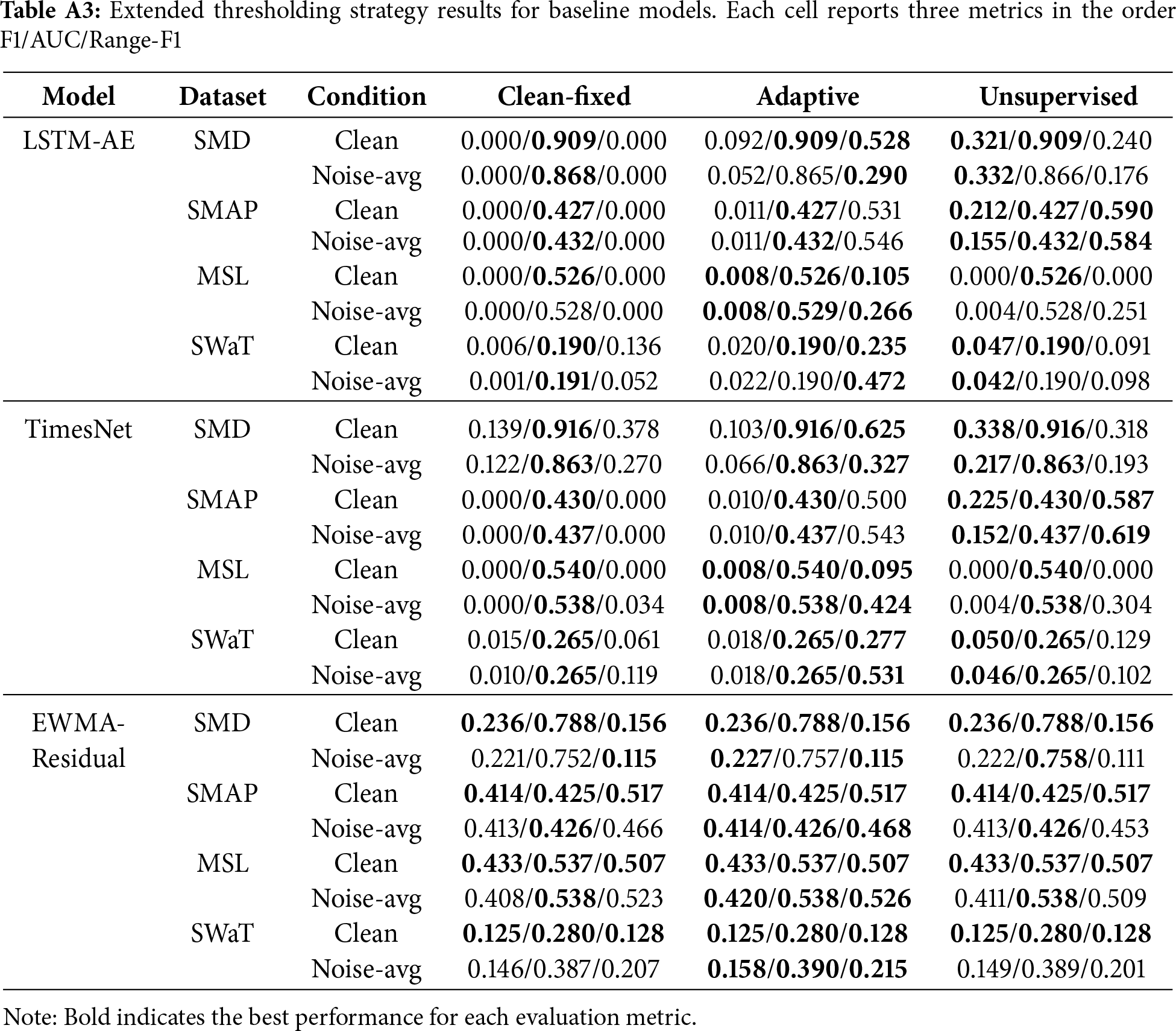
The Clean-fixed approach provides limited point-level detection. Across datasets, F1 values remain very low (often close to zero in cross-domain SMAP and MSL), although AUC scores remain stable. In SMD, Clean-fixed achieves relatively higher F1 and Range-F1 than in other datasets, but this comes largely from its in-domain advantage rather than thresholding effectiveness. Thus, Clean-fixed thresholds maximize coverage but severely limit usable precision, consistent with prior findings [8,9].

The Adaptive strategy produces more balanced outcomes. In SMD, F1 remains comparable to Clean-fixed (AnomalyTransformer: 0.160→0.106 under Clean), but Range-F1 increases substantially (up to 0.625). In cross-domain datasets, Adaptive consistently yields the highest Range-F1 values (e.g., SMAP ≈0.5, SWaT ≈0.35 in Noise-avg), indicating that adaptive thresholds enhance temporal coverage even when point-level accuracy remains weak.

The Unsupervised Adaptive strategy yields the strongest improvements in F1, especially under clean conditions. For instance, in SMD Clean, all three generative models see large F1 gains (AnomalyTransformer: 0.325, TranAD: 0.292, USAD: 0.329). Even in cross-domain SMAP and SWaT, Unsupervised thresholds recover non-trivial F1 where Clean-fixed completely collapses (e.g., SMAP-AnomalyTransformer: 0.208, TranAD: 0.234, USAD: 0.188). However, Range-F1 under Unsupervised is generally lower than Adaptive, suggesting a trade-off between precision-oriented detection and segment-level coverage.

Across models, AnomalyTransformer and TranAD show the clearest gains from Unsupervised thresholding in terms of F1, while USAD exhibits steadier but smaller improvements, reflecting relative insensitivity to threshold choice. These results confirm that thresholding is not a neutral post-processing step: depending on the strategy, the apparent robustness ranking of models can shift across both in-domain and cross-domain settings.

In summary:

•   Clean-fixed: stable but poor precision; F1 often ≈0 in cross-domain datasets.

•   Adaptive: consistently maximizes Range-F1 (segment coverage), even in cross-domain settings.

•   Unsupervised adaptive: best for boosting F1, especially in SMD and partially in SMAP/SWaT, but often at the cost of lower Range-F1.

Additional results for baseline models (LSTM-AE, TimesNet, EWMA-Residual) are reported in Appendix C. These baselines confirm broadly similar trade-offs, with generally smaller absolute gains from Unsupervised thresholding.

4.6 Summary of Robustness Patterns

Across Sections 4.1–4.5, several robustness patterns emerge that cut across datasets, noise types, design choices, and thresholding strategies.

First, model choice plays the most decisive role. AnomalyTransformer provides strong clean accuracy but deteriorates sharply under noise, TranAD maintains the most consistent robustness across domains, and USAD shows competitive clean performance yet suffers steep drops under structured perturbations. Among baselines, TimesNet balances accuracy and stability, LSTM-AE achieves moderate robustness with relatively low complexity, and EWMA-Residual often surpasses deep models in unstable domains, highlighting the enduring relevance of lightweight statistical baselines.

Second, dataset composition strongly modulates robustness. Within SMD, removing sensors disproportionately penalizes representation-heavy models, while server-group shifts occasionally mitigate degradation. Cross-domain transfers reveal divergent behaviors: in telemetry datasets (SMAP/MSL), lighter models and residual baselines often outperform complex architectures, whereas in attack-driven SWaT, residual detectors achieve exceptional stability.

Third, noise type and intensity dictate degradation profiles. Gaussian and Scaling drift perturbations remain relatively benign, while missing blocks degrade precision at high intensity. Spike and Mixed perturbations induce the steepest collapses, underscoring the need for resilience against abrupt, localized disruptions. USAD demonstrates relatively higher robustness under these challenging settings, though no model is universally resistant.

Fourth, architectural design choices such as window size and stride affect robustness asymmetrically. Mid-range window sizes (50–100) provide the most favorable trade-off, while very large windows (200) amplify noise sensitivity, especially for AnomalyTransformer. Stride variation exerts only minor influence, modestly increasing Detection Delay with minimal impact on robustness.

Finally, thresholding strategies significantly alter apparent robustness. Clean-fixed thresholds ensure coverage but collapse precision, Adaptive thresholds maximize segment-level Range-F1, and Unsupervised Adaptive thresholds boost F1 scores but trade off coverage. These shifts highlight that robustness is not an intrinsic model property alone but also a function of post-processing.

In summary:

•   Model dependence: TranAD is most consistently robust, while AnomalyTransformer and USAD are highly noise-sensitive in different ways; residual baselines remain surprisingly competitive.

•   Dataset effects: Feature composition and domain type shape robustness, with telemetry and attack-driven datasets favoring lighter or residual models.

•   Noise influence: Benign distortions contrast with disruptive spikes and mixed perturbations, where degradation is most severe.

•   Design choices: Window size dominates robustness outcomes, whereas stride plays only a minor role.

•   Thresholding impact: Post-processing strategies can reshape robustness rankings, underscoring their non-trivial role in evaluation.

These findings provide a consolidated view of robustness behavior and set the stage for deeper interpretation in Section 5.

5  Discussion

This section interprets the empirical results presented in Section 4, focusing on model-specific robustness patterns, trade-offs between sensitivity and stability, architectural insights, adversarial robustness, and practical deployment implications. It also situates the findings in the context of reviewer concerns regarding model scope, efficiency, and evaluation completeness.

5.1 Model-Specific Robustness Patterns

Generative AI models exhibit distinct robustness behaviors. AnomalyTransformer provides strong clean accuracy but collapses under noisy conditions, with degradation exceeding 65% in SMD. TranAD emerges as the most robust model overall, maintaining stability in both in-domain and cross-domain settings, particularly on MSL. USAD achieves competitive Range-F1 in clean telemetry but deteriorates sharply under structured perturbations such as missing blocks or mixed noise. These results echo prior findings that reconstruction-based models amplify noise sensitivity [1,2].

Among the baselines, TimesNet balances accuracy and stability [14], LSTM-AE shows moderate robustness with lower complexity, and EWMA-Residual occasionally outperforms deep models in unstable domains such as SWaT, supporting the argument that lightweight baselines remain competitive in noisy real-world conditions [46,47]. Other recent architectures, such as Autoformer [15] and the Non-stationary Transformer [16], were not included in the present evaluation but are expected to exhibit distinct robustness profiles; incorporating them remains a key direction for future benchmarking.

5.2 Trade-Offs between Sensitivity and Robustness

The results highlight a fundamental trade-off between sensitivity and robustness. Models such as AnomalyTransformer and USAD achieve strong clean detection but tend to over-react under noisy perturbations, leading to unstable performance. Conversely, models emphasizing stability, such as TranAD and EWMA-Residual, sometimes miss anomalies but maintain more consistent robustness across conditions. This sensitivity–robustness spectrum aligns with prior findings that anomaly detectors face an inherent trade-off under domain shift [23,48].

Beyond accuracy trade-offs, runtime and memory overheads also play a decisive role in deployability. Our profiling shows that lightweight models such as USAD and LSTM-AE achieve markedly shorter training times (∼167–191 s) and smaller GPU footprints (<130 MB), while Transformer-based models (AnomalyTransformer, TranAD) require nearly three times longer training (∼480 s) with higher memory demand (>150 MB). This implies that the robustness advantages of heavier architectures may be offset by efficiency constraints in latency- or resource-sensitive environments. Future evaluations should therefore jointly quantify detection delay, false alarm rate, and resource consumption to ensure actionable conclusions for real-world deployment [8]. Detailed runtime and memory profiling results are provided in Appendix D.

5.3 Architectural Insights from AD-Metrics

Architecture-level diagnostics clarify where robustness breaks down. First, in terms of frequency sensitivity, the Residual High-Frequency Ratio (HFR) should be interpreted such that lower values are more desirable, as high HFR denotes excessive sensitivity to spurious fluctuations. Across SMAP, MSL, and SWaT, the row-wise maxima in Tables A5–A11 consistently highlight EWMA-Residual as the most sensitive model, with TimesNet frequently peaking on SMD. AnomalyTransformer and TranAD exhibit mid-tier HFR overall, though they still show noticeable increases under disruptive perturbations (e.g., Spike, Mixed-sum/Mixed-block).

Second, representation stability (RS) should be read in the opposite direction: higher values are more desirable, as low RS indicates unstable latent spaces. USAD persistently records the row-wise minima on cross-domain datasets (SMAP, MSL, SWaT), indicating strong representational instability under distribution shift. By contrast, AnomalyTransformer, TranAD, and TimesNet retain comparatively higher RS.

Taken together, robustness degradation stems from two distinct architectural weaknesses. Classical residual baselines (and, on SMD, convolutional TimesNet) are most prone to frequency-domain over-sensitivity (high HFR), leading to sharp robustness drops under noisy conditions. In contrast, adversarially-trained Autoencoders (USAD) suffer from unstable latent representations (low RS), which explains their collapse under cross-domain evaluation. These diagnostics not only align with the Core-4 performance results but also motivate architecture-aware mitigation, such as frequency-robust filtering for residual baselines and stability-regularized training for latent Autoencoders.

5.4 Adversarial Perspective (KAGAN & ε-Sweep)

Beyond synthetic and mixed noise, robustness must also be assessed under adversarial threat models. GAN-based adversarial frameworks (e.g., KAGAN-style attacks) simulate structured perturbations aligned with model sensitivities [27–29]. Models that rely heavily on reconstruction discrepancies (e.g., AnomalyTransformer, USAD) may be more susceptible, whereas architectures with discriminative training signals such as TranAD are expected to exhibit relatively higher resilience.

To mitigate such vulnerabilities, adversarial training with an ε-curriculum—gradually increasing perturbation magnitude—has proven effective in stabilizing both image and time-series models [49,50]. An ε-sweep, where perturbation budgets are systematically varied, can further quantify adversarial margins.

5.5 Practical Recommendations for Model Selection

From a deployment perspective, model choice should reflect operational constraints. In stable industrial environments, AnomalyTransformer may be attractive due to its high clean accuracy, provided that noise robustness is not critical. For domains with unpredictable noise or cross-system transfer (e.g., spacecraft telemetry), TranAD offers the best trade-off between robustness and sensitivity. In security-critical infrastructures such as SWaT, lightweight residual detectors (e.g., EWMA-Residual) may outperform deep models by maintaining stability under adversarial-like perturbations. Practitioners should therefore prioritize robustness over marginal accuracy gains when anomalies carry high operational risk, consistent with guidelines for real-world anomaly detection deployment [46,48].

5.6 Limitations and Future Work

This study has several limitations. First, robustness evaluation focused on synthetic and mixed noise but did not yet include full-scale adversarial attacks such as KAGAN. Second, model training followed a uniform configuration, whereas domain-specific hyperparameter tuning could alter robustness outcomes. Third, evaluation was limited to SMD, SMAP, MSL, and SWaT; expanding to other industrial and medical datasets would broaden generalizability. Future work will address these gaps by integrating adversarial robustness experiments, exploring adaptive training curricula, and extending benchmarks to diverse architectures including Autoformer and Non-stationary Transformer. In addition, runtime and memory efficiency will be explicitly analyzed alongside accuracy. These directions will strengthen understanding of how generative and deep anomaly detectors operate under realistic, noisy, and adversarial conditions.

6  Conclusion

This study systematically evaluated the robustness of three representative generative time-series anomaly detectors—AnomalyTransformer, TranAD, and USAD—alongside baselines (LSTM-AE, EWMA-Residual) and a recent architecture (TimesNet). Evaluations were conducted under diverse noise types and intensities across SMD, SMAP, MSL, and SWaT, with further variations in window/stride, thresholding strategies, and architecture-level diagnostics. The objective was to quantify robustness degradation under realistic perturbations, provide fair model comparisons across domains, and extract actionable guidance for deployment.

The results highlight several important findings. TranAD consistently demonstrated the most stable performance across datasets and perturbations, whereas AnomalyTransformer achieved strong clean-set AUC but exhibited high sensitivity to noise. USAD remained competitive in clean telemetry but degraded substantially under structured perturbations, though it retained relative resilience under spike and mixed conditions. Lightweight residual-style baselines rivaled deep generative models in unstable or attack-driven domains such as SWaT. Noise type and intensity proved critical: Gaussian and Scaling drift were comparatively benign, Missing degraded precision at high intensity, and Spike/Mixed caused the steepest drops. Design choices also influenced robustness: mid-range windows (50–100) balanced localization and resilience, while very large windows (200) amplified noise sensitivity; stride had only marginal effects. Thresholding strategies were far from neutral: Clean-fixed often collapsed precision, Adaptive maximized segment coverage, and Unsupervised Adaptive yielded the strongest F1 gains. Finally, architecture-level diagnostics revealed that elevated Residual HFR coincided with robustness losses, and reduced Representation Stability explained failures in SMAP and parts of SWaT.

These findings carry several implications. For deployment, a robustness-first profile recommends TranAD as the default detector for cross-domain environments, with window sizes of 50–100 and stride between 1 and 5, and with Unsupervised Adaptive thresholding when point-level detection is paramount. Online monitoring of Residual HFR and Representation Stability can serve as early indicators of brittleness and guide adaptive recalibration. For evaluation standards, reporting both point- and segment-level metrics (F1, AUC, Range-F1, Delay, Drop%, and FAR) under clean and noise-averaged conditions is essential, together with a clear specification of noise taxonomy, intensity, window/stride, and thresholding strategy. For security-sensitive contexts, robustness-by-design measures such as adversarial curricula and periodic attack audits (e.g., KAGAN-style perturbations) are needed to ensure resilience under malicious manipulation.

Several limitations should be acknowledged. The present study emphasized naturalistic and mixed noise but did not include full adversarial evaluations; future work will incorporate systematic adversarial testing. Uniform training configurations ensured fairness but may not reflect domain-optimized performance, and structured ablations on hyperparameters remain necessary. Dataset coverage, while spanning four representative domains, should be extended to medical, IoT, and mobile sensing scenarios. Thresholding methods were limited to three strategies; distributionally robust and uncertainty-aware techniques (e.g., conformal prediction, score calibration) deserve further exploration. Runtime and memory profiling revealed notable efficiency gaps between lightweight autoencoder-style models and Transformer-based approaches, underscoring the need for efficiency-aware robustness benchmarks. Model scope should also expand to include Autoformer and the Non-stationary Transformer. Promising directions include frequency- or trend-aware attention, representation stabilization through contrastive or denoising objectives, test-time augmentation with ensembling, and adaptive windowing strategies responsive to dynamic noise regimes.

In closing, this work establishes a reproducible robustness benchmark for generative time-series anomaly detection and distills practical recommendations for real-world deployment. Beyond empirical reporting, the study advances the field methodologically by introducing a unified robustness protocol that integrates multi-metric evaluation with architecture-level diagnostics, analytically by demonstrating how noise types, design parameters, and thresholding strategies can reshape model rankings and quantifying the associated trade-offs, and practically by providing concrete guidelines for model selection, thresholding, and monitoring in noisy industrial deployments. Taken together, these findings underscore that while lightweight baselines can occasionally rival deep methods, the systematic comparison of the three generative AI models—AnomalyTransformer, TranAD, and USAD—remains the core contribution of this study, providing a robustness-centered benchmark of their relative strengths and weaknesses under noisy conditions. These contributions move the field beyond isolated accuracy benchmarks toward a principled understanding of robustness, offering both a foundation for reproducible research and a pathway to resilient, trustworthy anomaly detection in diverse cyber-physical systems.

Acknowledgement: The authors would like to thank SKKU SoftWare Lab for providing computing resources.

Funding Statement: This research was supported by the “Regional Innovation System & Education (RISE)” through the Seoul RISE Center, funded by the Ministry of Education (MOE) and the Seoul Metropolitan Government (2025-RISE-01-018-04). This research was also supported by the Korea Digital Forensic Center.

Author Contributions: The authors confirm contribution to the paper as follows: Conceptualization, Jeongsu Park and Moohong Min; methodology, Jeongsu Park; software, Jeongsu Park; validation, Jeongsu Park; formal analysis, Jeongsu Park; investigation, Jeongsu Park; resources, Jeongsu Park; data curation, Jeongsu Park; writing—original draft preparation, Jeongsu Park; writing—review and editing, Jeongsu Park and Moohong Min; visualization, Jeongsu Park; supervision, Moohong Min; project administration, Moohong Min. All authors reviewed the results and approved the final version of the manuscript.

Availability of Data and Materials: The data that support the findings of this study are openly available. The Server Machine Dataset (SMD) used in this research is publicly accessible at the official repository: https://github.com/NetManAIOps/OmniAnomaly (accessed on 12 October 2025). The NASA spacecraft telemetry datasets, SMAP and MSL, are publicly available at the Telemanom repository: https://github.com/khundman/telemanom (accessed on 12 October 2025). The Secure Water Treatment (SWaT) dataset is provided by the iTrust Centre for Research in Cyber Security, Singapore University of Technology and Design (SUTD): https://itrust.sutd.edu.sg/itrust-labs_datasets/ (accessed on 12 October 2025).

Ethics Approval: Not applicable.

Conflicts of Interest: The authors declare no conflicts of interest to report regarding the present study.

Appendix A Additional Results on Baseline Selection

This appendix provides the detailed results of baseline screening experiments, which motivated the choice of LSTM-AE and EWMA-Residual as the two retained baselines. As described in Section 3.5, several classical baselines (LSTM-AE, TimesNet, EWMA-Residual, Z-Score, VAE, Isolation Forest) were initially included to ensure methodological diversity. To systematically compare them, we conducted evaluation under multiple representative conditions: Clean, Gaussian-middle, and Spike-middle on the concatenated SMD (1-1/1-2/1-3) dataset with window size 50 and stride 1.

Table A1 reports F1, AUC, and NAB metrics. Across all conditions, LSTM-AE and EWMA-Residual consistently ranked within the top-2, while other baselines such as VAE or Z-Score occasionally performed well in individual metrics but lacked stability across scenarios. In particular, EWMA-Residual showed robust average performance, while LSTM-AE remained competitive even under noise (e.g., Gaussian-middle, Spike-middle). Therefore, these two baselines were carried forward for the main experiments in Section 4, ensuring both empirical competitiveness and methodological complementarity.

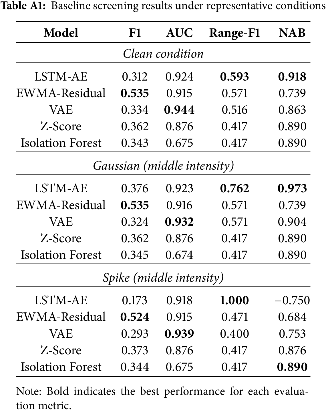
To further validate consistency, Table A2 summarizes the average ranking of each baseline across all conditions. LSTM-AE and EWMA-Residual maintain the lowest (best) average ranks, confirming their stability and justifying their retention as the top-2 baselines.

Appendix B Additional Results on Noise Intensity

This appendix reports the full set of noise—intensity plots for completeness. Figs. A1–A5 complement the main text (Section 4.3), which only highlighted Spike (Fig. 6) and Mixed-sum (Fig. 7) as representative cases.

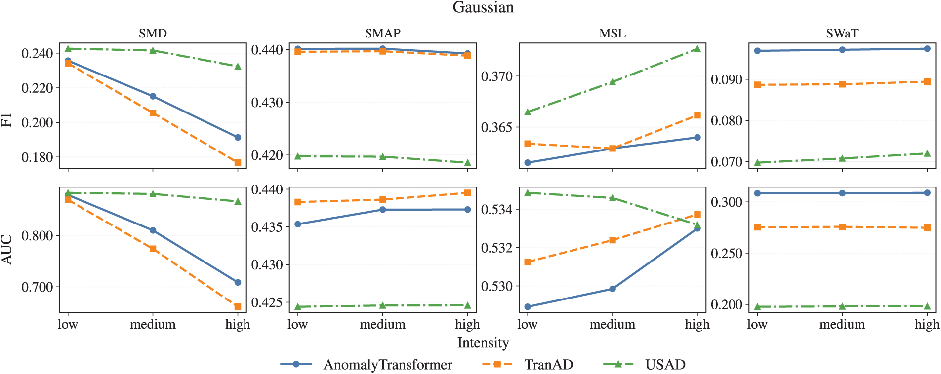
Figure A1: Gaussian noise across three intensity levels

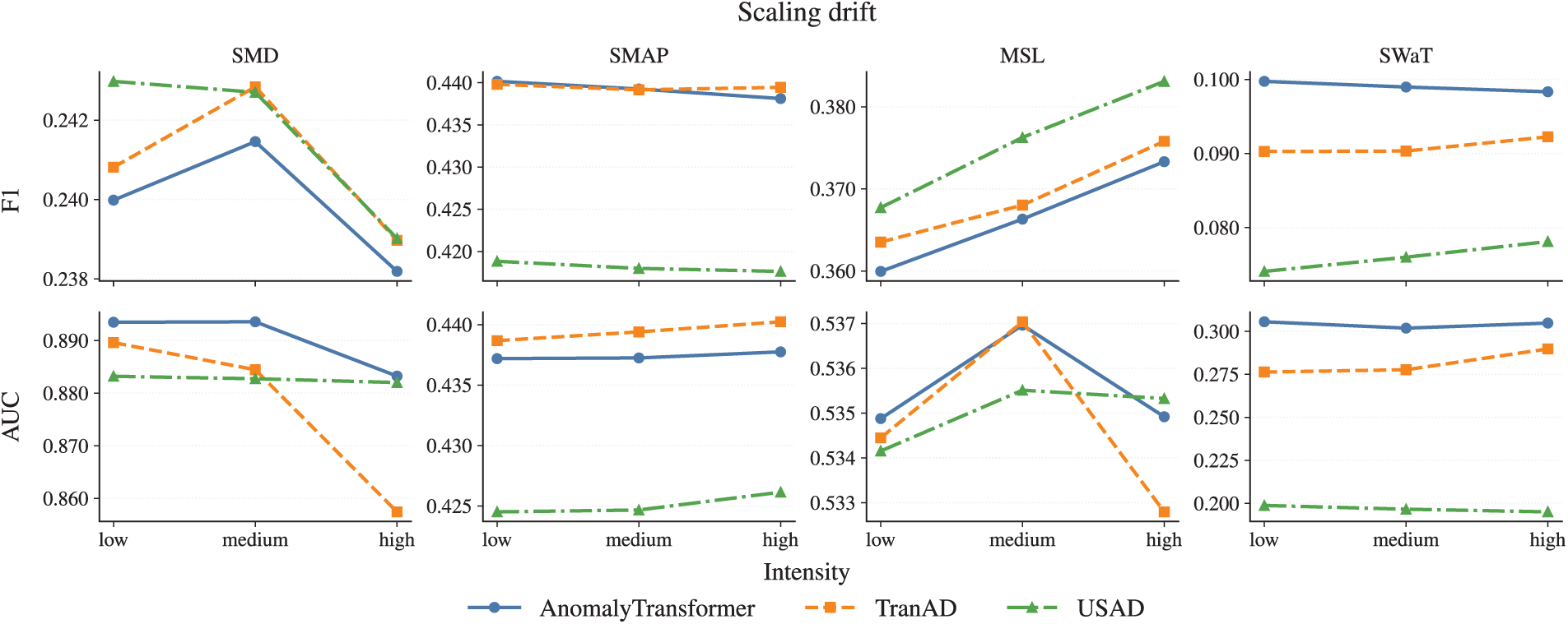
Figure A2: Scaling drift noise across three intensity levels

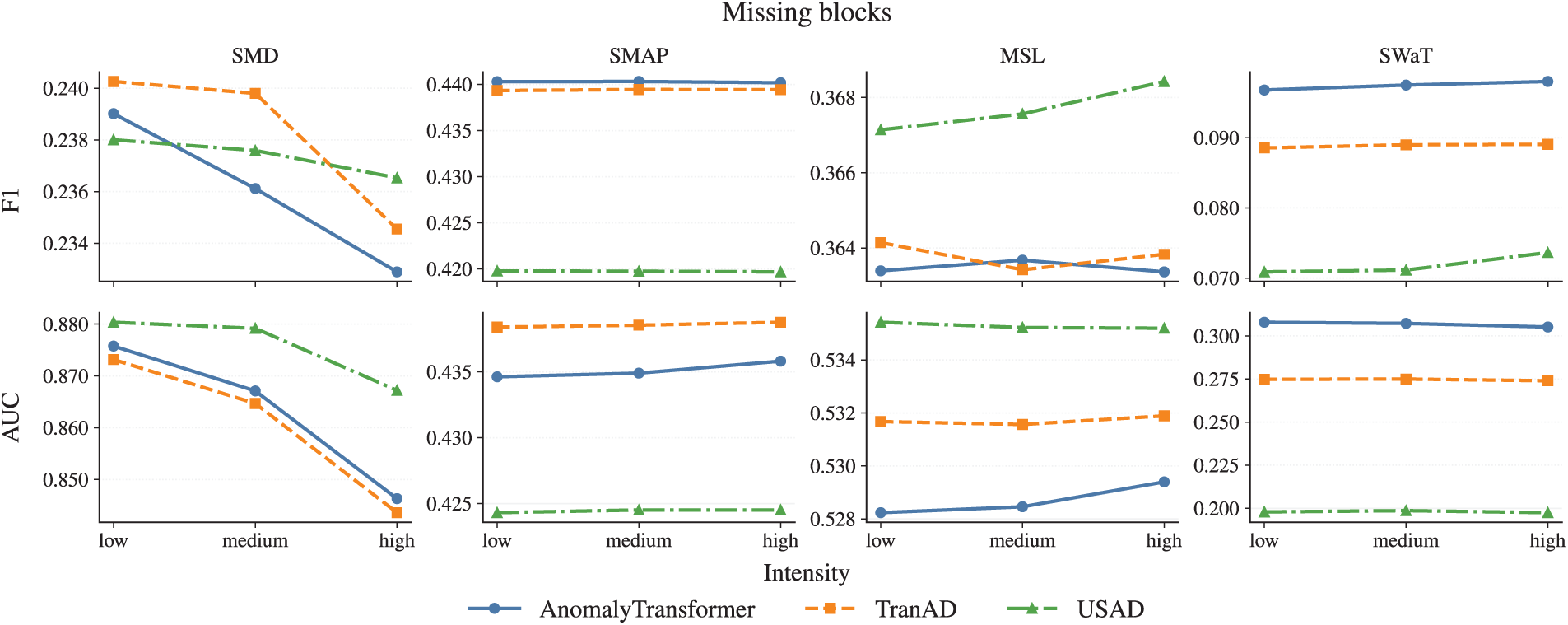
Figure A3: Missing blocks noise across three intensity levels

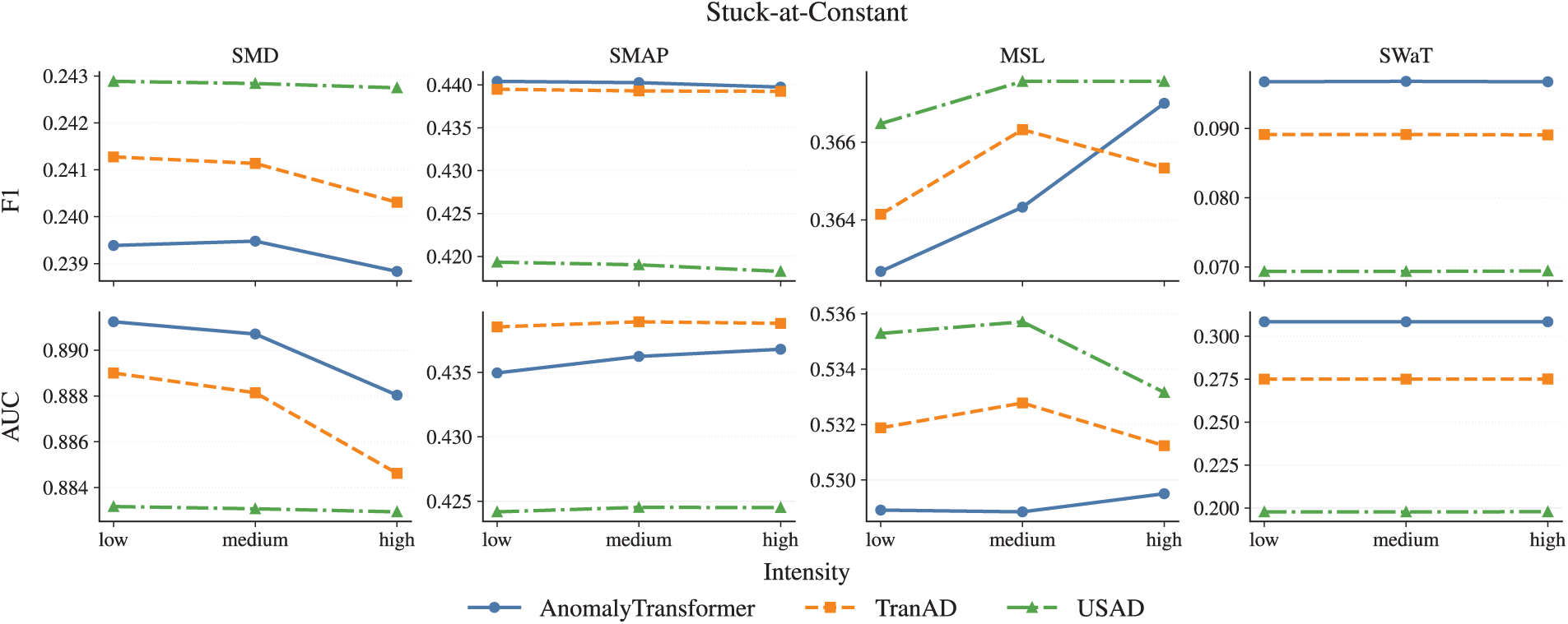
Figure A4: Stuck-at-Constant noise across three intensity levels

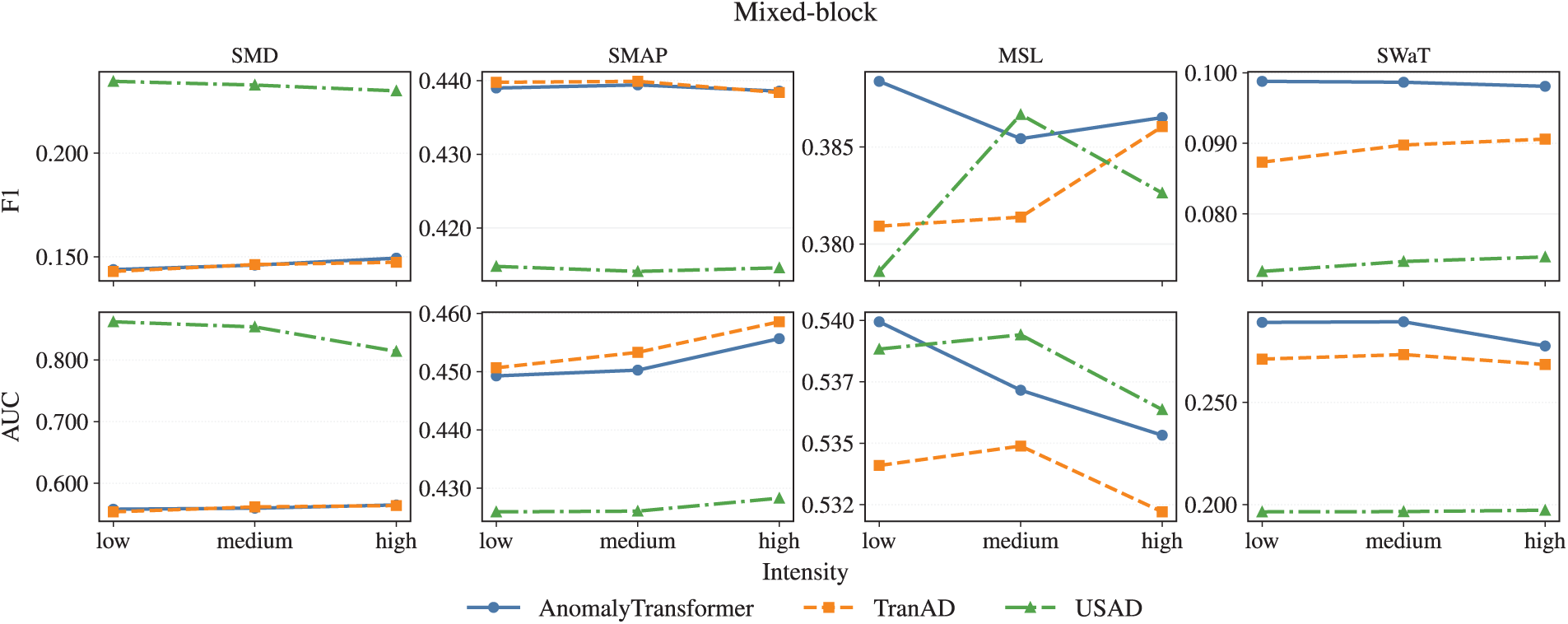
Figure A5: Mixed-block noise across three intensity levels

Appendix C Additional Results on Thresholding Strategies

This appendix provides the extended comparison of thresholding strategies across all models and datasets. Table A3 complements the main text (Section 4.5), where only the three representative generative models (AnomalyTransformer, TranAD, USAD) were highlighted in Table 6. The additional results for the baseline models (LSTM-AE, TimesNet, EWMA-Residual) are reported here for completeness.

Appendix D Additional Results on Runtime and Efficiency Metrics

This appendix complements Sections 5.3 and 4.4 by reporting full quantitative results on runtime and memory efficiency. Whereas the main text discussed robustness and architectural diagnostics qualitatively, here we provide a detailed comparison of training cost, inference efficiency, and GPU memory usage across all baseline models. These measurements were obtained on identical hardware under consistent training settings (20 epochs, batch size =128).

Table A4 summarizes parameter counts, parameter size, wall-clock training time, peak GPU memory usage, FLOPs per forward pass, and inference efficiency (latency for a single window at batch size =1, and throughput for batch size =32).

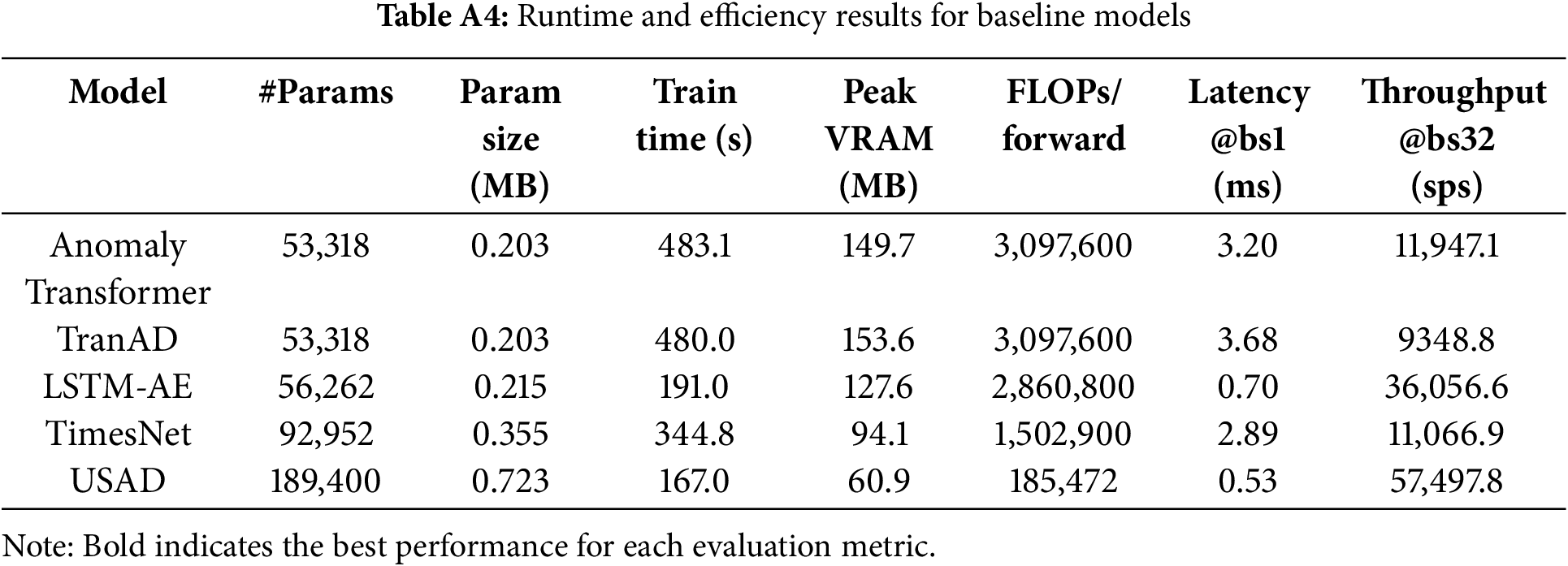
Several key observations emerge:

•   Transformer-based models (AnomalyTransformer, TranAD) are the most resource-intensive, requiring nearly 480 s training time and >150 MB VRAM, confirming that robustness advantages may come at the cost of efficiency.

•   Lightweight baselines such as USAD and LSTM-AE complete training substantially faster (∼167–191 s) and with smaller memory footprints (<130 MB), while achieving very high throughput (e.g., >36,000 samples/sec for LSTM-AE).

•   TimesNet sits in between: it is more efficient than Transformers in both VRAM and training time, but still heavier than USAD or LSTM-AE.

These results illustrate that runtime and memory overheads form a second trade-off axis that must be considered alongside robustness and sensitivity (Section 5). While heavy Transformer architectures may offer robustness benefits, lighter models remain attractive in latency-sensitive or resource-constrained deployments.

Appendix E Additional Results on Architectural Metrics

This appendix reports the full architecture-level metrics that complement the main discussion in Section 5.3. While the main text focused on qualitative patterns of Residual High-Frequency Ratio (HFR) and Representation Stability (RS), here we provide the complete quantitative results across all models (AnomalyTransformer, TranAD, USAD, LSTM-AE, TimesNet, EWMA-Residual), datasets (SMD, SMAP, MSL, SWaT), and noise conditions (Clean, Gaussian, Spike, Missing blocks, Stuck-at-Constant, Scaling drift, Mixed-sum, Mixed-block).

Tables A5–A11 summarize the HFR values, where higher ratios indicate stronger sensitivity to spurious fluctuations. For each noise type, the maximum HFR within a row is boldfaced to highlight the most sensitive model.

Tables A6–A12 report the RS values, where numbers closer to 1.0 denote stable latent representations. The minimum RS within each row is boldfaced to identify the least stable model under the given noise perturbation. For EWMA-Residual, RS values are not defined and thus omitted (denoted as “–”).

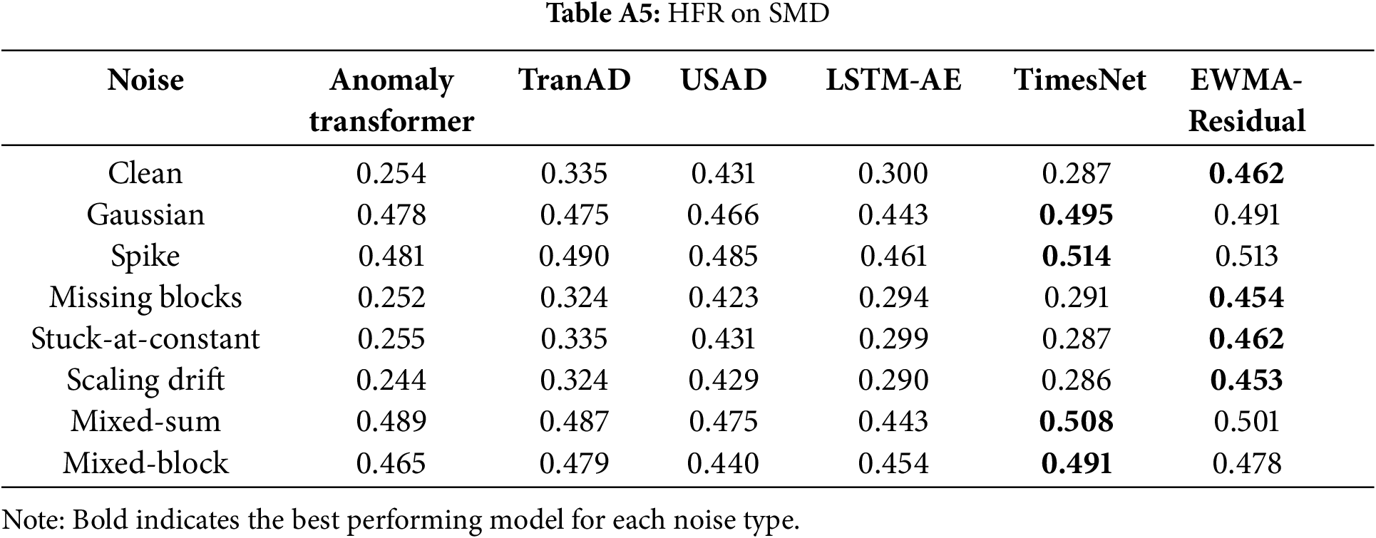
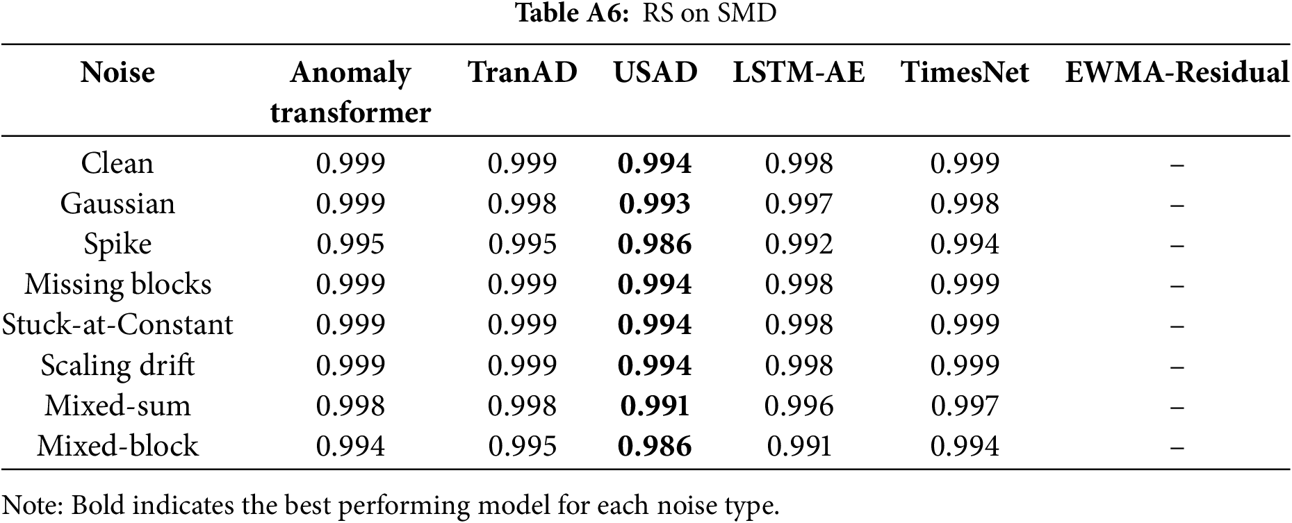
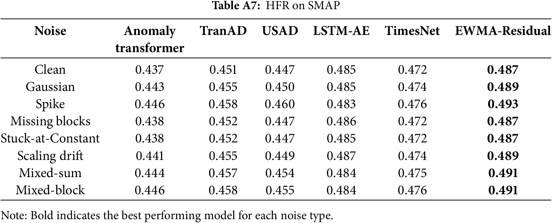
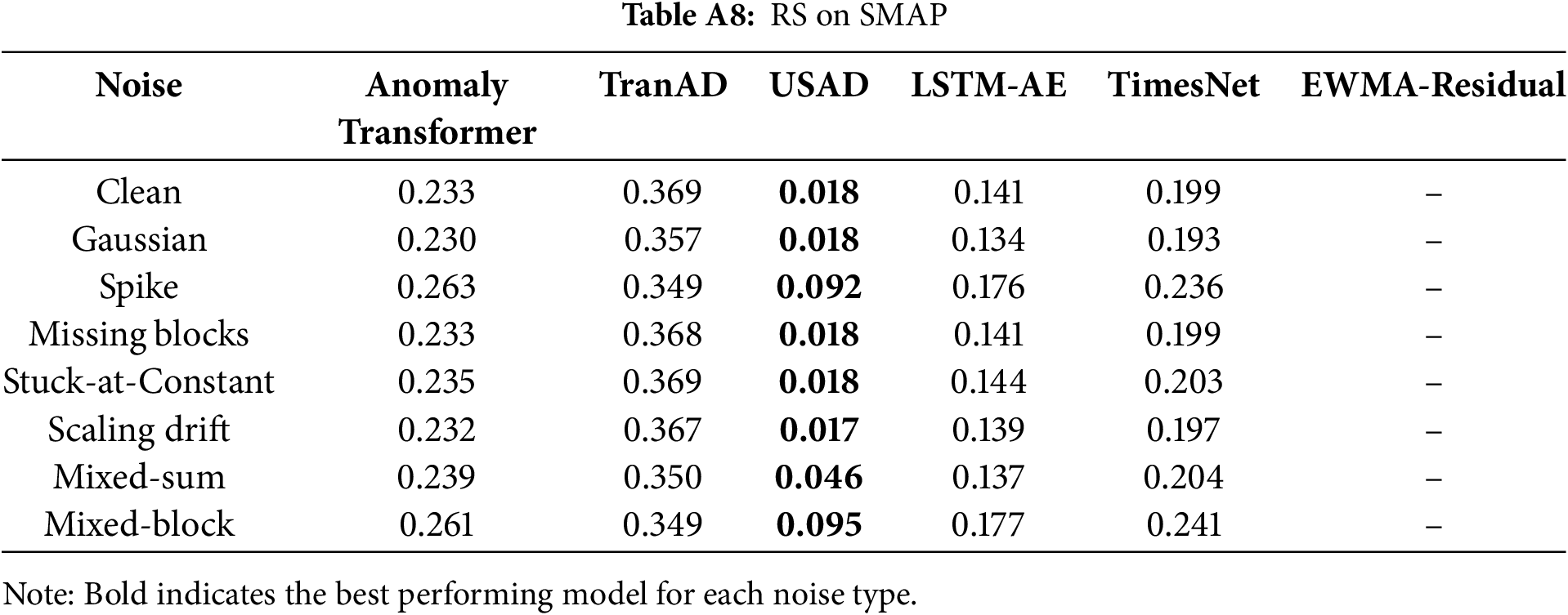
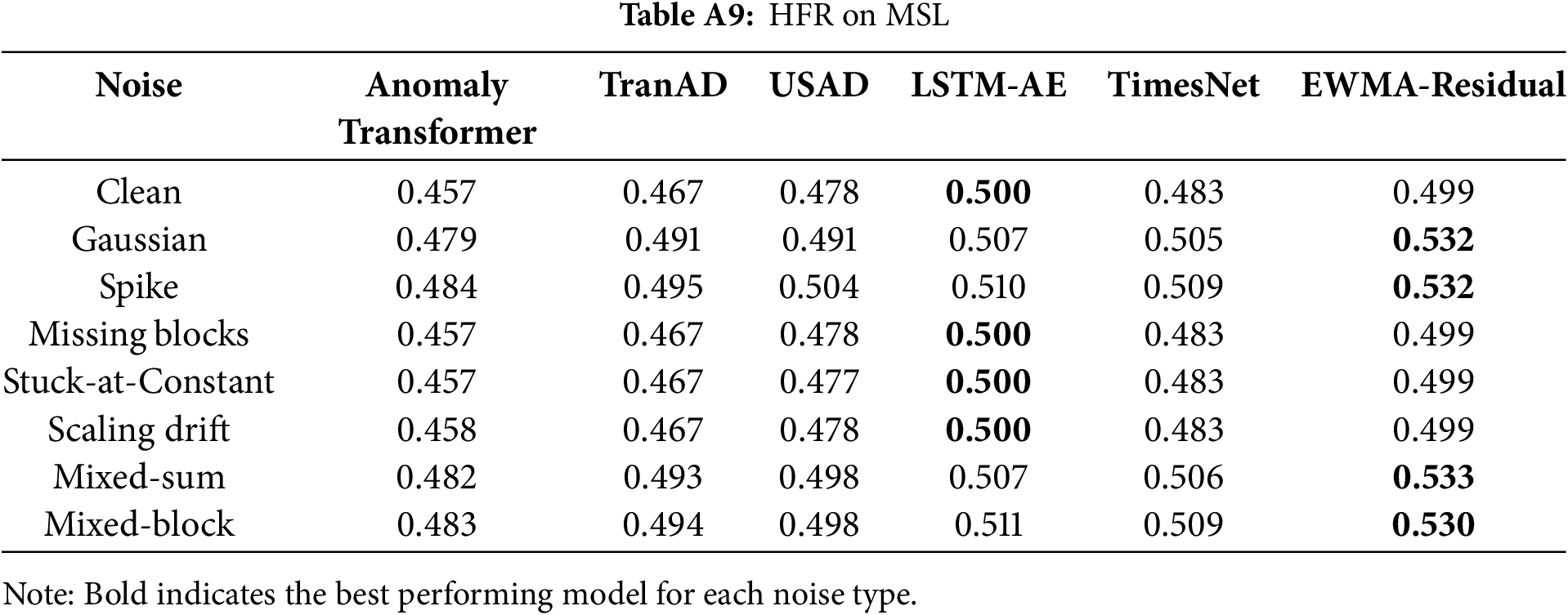
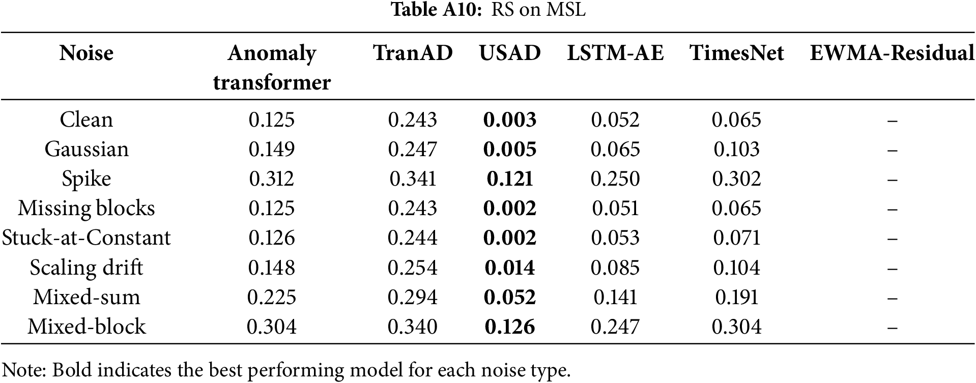
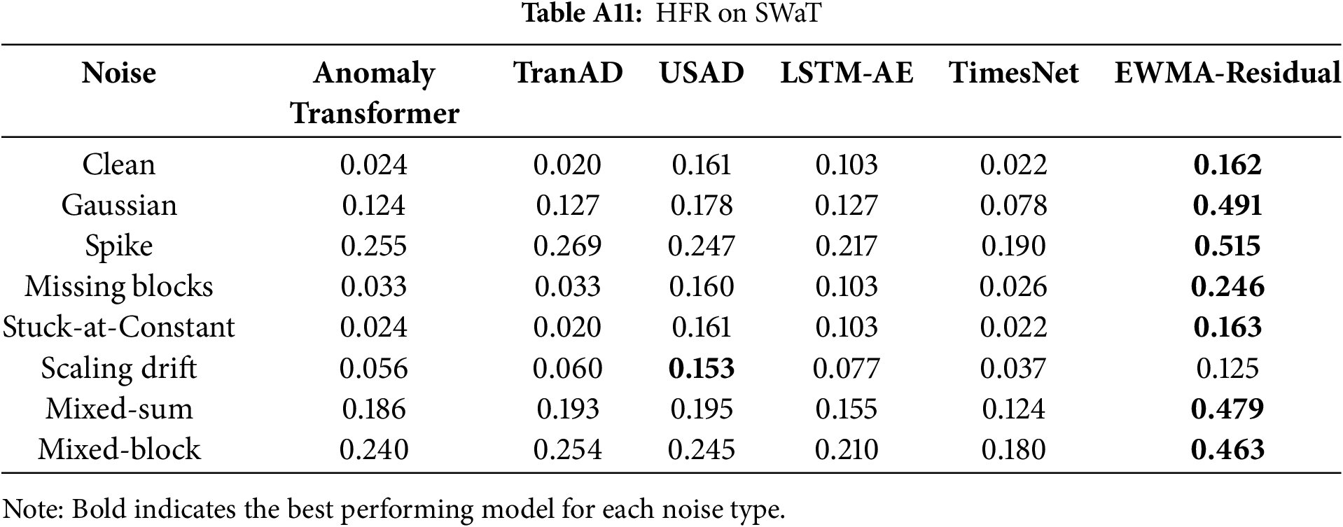
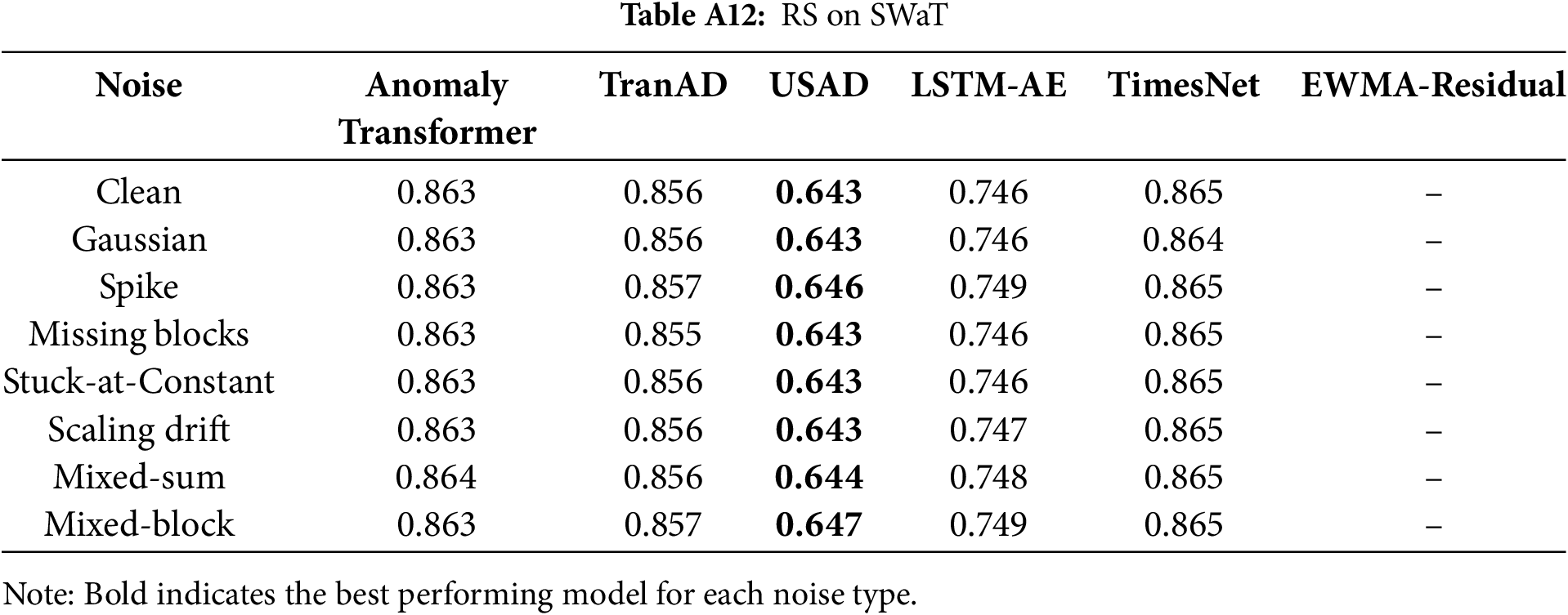
Together, these extended results provide detailed evidence for the architectural robustness analysis, supporting the observations in Section 5.3 that (i) Transformer-based models tend to exhibit inflated HFR under noise, reflecting heightened sensitivity to high-frequency perturbations, and (ii) cross-domain telemetry datasets such as SMAP and MSL reveal substantial instability in representation space.

References

1. Mejri N, Lopez-Fuentes L, Roy K, Chernakov P, Ghorbel E, Aouada D. Unsupervised anomaly detection in time-series: an extensive evaluation and analysis of state-of-the-art methods. Expert Syst Appl. 2024;256(5):124922. doi:10.1016/j.eswa.2024.124922. [Google Scholar] [CrossRef]

2. Schmidl S, Wenig P, Papenbrock T. Anomaly detection in time series: a comprehensive evaluation. Proc VLDB Endowment. 2022;15(9):1779–97. doi:10.14778/3538598.3538602. [Google Scholar] [CrossRef]

3. Xu J, Wu H, Wang J, Long M. Anomaly transformer: time series anomaly detection with association discrepancy. arXiv:2110.02642. 2022. [Google Scholar]

4. Tuli S, Casale G, Jennings NR. TranAD: deep transformer networks for anomaly detection in multivariate time series data. Proc VLDB Endowment. 2022;15(6):1201–14. [Google Scholar]

5. Audibert J, Michiardi P, Guyard F, Marti S, Zuluaga MA. USAD: unsupervised anomaly detection on multivariate time series. In: Proceedings of the 26th ACM SIGKDD International Conference on Knowledge Discovery and Data Mining; 2020 Jul 6–10; Online. New York, NY, USA: ACM. p. 3395–404. [Google Scholar]

6. Su Y, Zhao Y, Niu C, Liu R, Sun W, Pei D. Robust anomaly detection for multivariate time series through stochastic recurrent neural network. In: Proceedings of the 25th ACM SIGKDD International Conference on Knowledge Discovery & Data Mining (KDD); 2019 Aug 4–8; Anchorage, AK, USA. New York, NY, USA: ACM. p. 2828–37. [Google Scholar]

7. Hundman K, Constantinou V, Laporte C, Colwell I, Soderstrom T. Detecting spacecraft anomalies using LSTMs and nonparametric dynamic thresholding. In: Proceedings of the 24th ACM SIGKDD International Conference on Knowledge Discovery & Data Mining (KDD); 2018 Aug 19–23; London, UK. New York, NY, USA: ACM. p. 387–95. [Google Scholar]

8. Kim S, Yoon S, Gwon Y. Towards a rigorous evaluation protocol for time-series anomaly detection. In: 36th AAAI Conference on Artificial Intelligence (AAAI-22); 2022 Feb 22–Mar 1; Online. Palo Alto, CA, USA: AAAI Press; 2022. p. 12395–402. [Google Scholar]

9. Paparrizos J, Boniol P, Palpanas T, Tsay RS, Elmore AJ, Franklin MJ. Volume under the surface: a new accuracy evaluation measure for time-series anomaly detection. Proc VLDB Endowment. 2022;15(11):2774–87. doi:10.14778/3551793.3551830. [Google Scholar] [CrossRef]

10. Sørbø P, Ruocco M. Navigating the Metric Maze: a taxonomy of evaluation metrics for anomaly detection in time series. Data Min Knowl Discov. 2023;37(5):1705–38. doi:10.1007/s10618-023-00988-8. [Google Scholar] [CrossRef]

11. Wang F, Jiang Y, Zhang R, Wei A, Xie J, Pang X. A survey of deep anomaly detection in multivariate time series: taxonomy, applications, and directions. Sensors. 2025;25(1):190. doi:10.3390/s25010190. [Google Scholar] [PubMed] [CrossRef]

12. Wang R, Zhou Y, Luo G, Chen P, Peng D. Cross-dimension attentive feature fusion network for unsupervised time-series anomaly detection. Comput Model Eng Sci. 2024;139(3):3011–27. doi:10.32604/cmes.2023.047065. [Google Scholar] [CrossRef]

13. Malhotra P, Ramakrishnan A, Anand G, Vig L, Agarwal P, Shroff G. LSTM-based encoder-decoder for multi-sensor anomaly detection. arXiv:1607.00148. 2016. [Google Scholar]

14. Wu H, Hu T, Liu Y, Zhou H, Wang J, Long M. TimesNet: temporal 2D-variation modeling for general time series analysis. arXiv:2210.02186. 2023. [Google Scholar]

15. Wu H, Xu J, Wang J, Long M. Autoformer: decomposition transformers with auto-correlation for long-term series forecasting. In: Advances in neural information processing systems (NeurIPS). Vol. 34. Red Hook, NY, USA: Curran Associates, Inc.; 2021. p. 22419–30. [Google Scholar]

16. Liu Y, Wu H, Wang J, Long M. Non-stationary transformers: exploring the stationarity in time series forecasting. arXiv:2205.14415. 2022. [Google Scholar]

17. Golyandina N, Nekrutkin V, Zhigljavsky A. Analysis of time series structure: SSA and related techniques. Boca Raton, FL, USA: Chapman and Hall/CRC [Internet]. 2001 [cited 2025 Oct 1]. Available from: https://www.taylorfrancis.com/books/mono/10.1201/9780367801687/analysis-time-series-structure-nina-golyandina-vladimir-nekrutkin-anatoly-zhigljavsky. [Google Scholar]

18. Wang Y, Cheng H, Xiong J, Wen Q, Jia H, Song R, et al. Noise-resilient point-wise anomaly detection in time series using weak segment labels. In: Proceedings of the 31st ACM SIGKDD Conference on Knowledge Discovery and Data Mining; 2025 Aug 3–7; Toronto, ON, Canada. New York, NY, USA: ACM. p. 1551–62. [Google Scholar]

19. Zhang X, Xu S, Chen H, Chen Z, Zhuang F, Xiong H, et al. Rethinking robust multivariate time series anomaly detection: a hierarchical spatio-temporal variational perspective. IEEE Trans Knowl Data Eng. 2024;36(12):9136–49. doi:10.1109/tkde.2024.3466291. [Google Scholar] [CrossRef]

20. Shon J. Toward a robust approach to multivariate time series anomaly detection [Internet]. 2025 [cited 2025 Oct 1]. Available from: https://www.spiedigitallibrary.org/conference-proceedings-of-spie/13426/3050401/Toward-a-robust-approach-to-multivariate-time-series-anomaly-detection/10.1117/12.3050401.short. [Google Scholar]

21. Li G, Yang Z, Wan H, Li M. Anomaly-PTG: a time series data-anomaly-detection transformer framework in multiple scenarios. Electronics. 2022;11(23):3955. doi:10.3390/electronics11233955. [Google Scholar] [CrossRef]

22. Khoshnevisan F, Fan Z, Carvalho VR. Improving robustness on seasonality-heavy multivariate time series anomaly detection. arXiv:2007.14254. 2020. [Google Scholar]

23. Han S, Ding Y, Zhao Y, Liu Z, Yin Y, Wang S, et al. ADBench: anomaly detection benchmark. arXiv:2206.09426. 2022. [Google Scholar]

24. Si H, Li J, Pei C, Cui H, Yang J, Sun Y, et al. TimeSeriesBench: an industrial-grade benchmark for time series anomaly detection models. In: 2024 IEEE 35th International Symposium on Software Reliability Engineering (ISSRE); 2024 Oct 28–31; Tsukuba, Japan. p. 61–72. [Google Scholar]

25. Schmidl S, Kästner J, Wenig P, Papenbrock T. TimeEval: a benchmarking toolkit for time series anomaly detection algorithms. Proc VLDB Endowment. 2022;15(11):3678–81. [Google Scholar]

26. Paparrizos J, Kang Y, Boniol P, Tsay RS, Palpanas T, Franklin MJ. TSB-UAD: an end-to-end benchmark suite for univariate time-series anomaly detection. Proc VLDB Endowment. 2022;15(8):1697–711. [Google Scholar]

27. Fawaz HI, Lucas B, Forestier G, Pelletier C, Schmidt DF, Weber J, et al. Adversarial attacks on deep neural networks for time series classification. In: 2019 International Joint Conference on Neural Networks (IJCNN); 2019 Jul 14–19; Budapest, Hungary. p. 1–8. [Google Scholar]

28. Xiao C, Li B, Zhu JY, He W, Liu M, Song D. Generating adversarial examples with adversarial networks. In: Proceedings of the 27th International Joint Conference on Artificial Intelligence (IJCAI); 2018 Jul 13–19. Stockholm, Sweden. p. 3905–11. [Google Scholar]

29. Bashar A, Akter T, Kim JS, Lee JW. ALGAN: time series anomaly detection with adjusted-LSTM GAN. J Big Data. 2025;12(1):1–22. doi:10.21203/rs.3.rs-3609809/v1. [Google Scholar] [CrossRef]

30. Saravanan S, Kumar P, Rajasekaran S, Subramanian R. TSI-GAN: unsupervised time series anomaly detection using convolutional cycle-consistent GANs. arXiv:2303.12952. 2023. [Google Scholar]

31. Belkhouja T, Doppa JR. Adversarial framework with certified robustness for time-series domain via statistical features. J Artif Intell Res. 2022;73:1435–71. doi:10.1613/jair.1.13543. [Google Scholar] [CrossRef]

32. Komadina A, Martinić M, Groš S, Mihajlović V. Comparing threshold selection methods for network anomaly detection. IEEE Access. 2024;12:124943–73. doi:10.1109/access.2024.3452168. [Google Scholar] [CrossRef]

33. Mathur AP, Tippenhauer NO. SWaT: a water treatment testbed for research and training on ICS security. In: 2016 International Workshop on Cyber-Physical Systems for Smart Water Networks (CySWater); 2016 Apr 11; Vienna, Austria. p. 31–6. doi:10.1109/CySWater.2016.7469060. [Google Scholar] [CrossRef]

34. Yue W, Ying X, Guo R, Chen D, Shi J, Xing B, et al. Sub-adjacent transformer: improving time series anomaly detection with reconstruction error from sub-adjacent neighborhoods. arXiv:2404.18948. 2024. [Google Scholar]

35. Tuptuk N, Hazell P, Watson J, Hailes S. A systematic review of the state of cyber-security in water systems. Water. 2021;13(1):81. doi:10.3390/w13010081. [Google Scholar] [CrossRef]

36. Ma X, Li Z, Yang T, Xie W, Wang M, Chen E. SMIL: multimodal learning with severely missing modality. In: Proceedings of the 35th AAAI Conference on Artificial Intelligence; 2021 Feb 2–9; Online. p. 8613–21. [Google Scholar]

37. John J, Kawanishi T. A multimodal sensor fusion framework robust to missing modalities for person recognition. arXiv:2210.10972. 2022. [Google Scholar]

38. Wang X, Zhou Y, Zhang P, Li X, Yang Y. Multi-modal learning with missing modality via shared-specific feature modelling. In: Proceedings of the 2023 IEEE/CVF Conference on Computer Vision and Pattern Recognition (CVPR); 2023 Jun 17–24; Vancouver, BC, Canada. p. 15802–11. [Google Scholar]

39. Roheda S, Riggan BS, Krim H, Dai L. Cross-modality distillation: a case for conditional generative adversarial networks. arXiv:1807.07682. 2018. [Google Scholar]

40. Wu R, Wang H, Chen H, Carneiro G. Deep multimodal learning with missing modality: a survey. arXiv:2409.07825. 2024. [Google Scholar]

41. Sharma S, Gupta K, Gupta D, Rani S, Dhiman G. An insight survey on sensor errors and fault detection techniques in smart spaces. Comput Model Eng Sci. 2024;138(3):2029–59. doi:10.32604/cmes.2023.029997. [Google Scholar] [CrossRef]

42. Wang Y, Yang A, Chen X, Wang P, Wang Y, Yang H. A deep learning approach for blind drift calibration of sensor networks. arXiv:1707.03682. 2017. [Google Scholar]

43. Qiu X, Li Z, Qiu W, Hu S, Zhou L, Wu X, et al. TAB: unified benchmarking of time series anomaly detection methods. arXiv:2506.18046. 2025. [Google Scholar]

44. Liu Q, Paparrizos J. The elephant in the room: towards a reliable time-series anomaly detection benchmark. In: Advances in neural information processing systems. Vol. 37. Red Hook, NY, USA: Curran Associates, Inc.; 2024. p. 108231–61. [Google Scholar]

45. Paparrizos J, Boniol P, Liu Q, Palpanas T. Advances in time-series anomaly detection: algorithms, benchmarks, and evaluation measures. In: Proceedings of the 31st ACM SIGKDD Conference on Knowledge Discovery and Data Mining V.2; 2025 Aug 3–7; Toronto, ON, Canada. p. 6151–61. [Google Scholar]

46. Laptev N, Yosinski J, Li LE, Smyl S. Time-series extreme event forecasting with neural networks at Uber. In: Proceedings of the ICML 2017 Time Series Workshop; 2017 Aug; Sydney, Australia. [cited 2025 Oct 1]. Available from: https://openreview.net/forum?id=BKiWXX3Liz. [Google Scholar]

47. Zong B, Song Q, Min MR, Cheng W, Lumezanu C, Cho D, et al. Deep autoencoding gaussian mixture model for unsupervised anomaly detection. In: International Conference on Learning Representations (ICLR) [Internet]; 2018 Feb 16; Vancouver, BC, Canada. [cited 2025 Oct 1]. Available from: https://openreview.net/forum?id=BJJLHbb0-. [Google Scholar]

48. Blázquez-García A, Conde A, Mori U, Lozano JA. A review on outlier/anomaly detection in time series data. ACM Comput Surv. 2021;54(3):56. doi:10.1145/3444690. [Google Scholar] [CrossRef]

49. Madry A, Makelov A, Schmidt L, Tsipras D, Vladu A. Towards deep learning models resistant to adversarial attacks. In: International Conference on Learning Representations (ICLR) [Internet]; 2018 Feb 16; Vancouver, BC, Canada. [cited 2025 Oct 1]. Available from: https://openreview.net/forum?id=rJzIBfZAb. [Google Scholar]

50. Zhang H, Yu Y, Jiao J, Xing E, Ghaoui LE, Jordan M. Theoretically principled trade-off between robustness and accuracy. In: Proceedings of the 36th International Conference on Machine Learning; 2019 Jun 9–15; Long Beach, CA, USA. p. 7472–82. [cited 2025 Oct 1]. Available from: https://proceedings.mlr.press/v97/zhang19p.html. [Google Scholar]